

Introduction
A multitude of features known as rock glaciers and/or debris-covered glaciers are observed in alpine environments over a wide range of latitudes on Earth. These features typically have a tongue-like or lobate plan form and advance through internal deformation and/or basal sliding at relatively low flow velocities. Their internal composition consists almost entirely of ice and rock debris, although the proportions and sources of these two components can be highly variable. They have been the subject of nearly a century of field, laboratory and modeling research, but fundamental questions remain about their formation and evolution.
Much of the confusion associated with rock glaciers and debris-covered glaciers exists because of the broad range of features that display some of their common characteristics. Conflicting nomenclature and classification schemes have further complicated the situation. Here we define debris-covered glaciers as features that consist of a demonstrable core of relatively clean glacier ice covered by a thin (cm to m scale) layer of debris (e.g. Reference PotterPotter, 1972; Reference Clark, Clark and GillespieClark and others, 1994; Reference AckertAckert, 1998; Reference Potter, Steig, Clark, Speece, Clark and UpdikePotter and others, 1998; Reference Konrad, Humphrey, Steig, Clark, Potter and PfefferKonrad and others, 1999; Reference Krainer, Mostler and SpanKrainer and others, 2002). This definition distinguishes these features from those commonly referred to as rock glaciers, that typically, in whole or in part, consist of debris mobilized by flow of interstitial ice of secondary origin (e.g. Reference Wahrhaftig and CoxWahrhaftig and Cox, 1959; Reference WhiteWhite, 1976; Reference Hassinger and MayewskiHassinger and Mayewski, 1983; Reference HaeberliHaeberli, 1985; Reference Barsch, Giardino, Shroder and VitekBarsch, 1987; Reference Whalley and AziziWhalley and Azizi, 2003). While previous studies have suggested that rock glaciers and debris-covered glaciers may be intrinsically related or may simply represent end members of a diverse continuum, we believe that in some situations they possess unique formation processes and deformation mechanisms. For excellent reviews of rock glaciers, debris-covered glaciers and their classification, we refer the reader to Reference Wahrhaftig and CoxWahrhaftig and Cox (1959), Reference Martin and WhalleyMartin and Whalley (1987), Reference Whalley and MartinWhalley and Martin (1992), Reference Hamilton and WhalleyHamilton and Whalley (1995), Reference Nakawo, Raymond and FountainNakawo and others (2000) and Reference Whalley and AziziWhalley and Azizi (2003).
Regardless of classification or formative mechanism, there is general agreement that rock glaciers and debris-covered glaciers contain valuable climatological data. Several recent studies have shown that debris-covered glaciers have the potential to store long-term climate records (Reference Clark, Steig, Potter and GillespieClark and others, 1998; Reference Steig, Fitzpatrick, Potter and ClarkSteig and others, 1998; Reference HaeberliHaeberli and others, 1999; Reference Konrad, Humphrey, Steig, Clark, Potter and PfefferKonrad and others, 1999). These records can be extracted through isotopic analyses of ice cores/samples (Reference Clark, Steig, Potter and GillespieClark and others, 1998; Reference Steig, Fitzpatrick, Potter and ClarkSteig and others, 1998) and potentially through morphological analyses of surface features (Reference AckertAckert, 1998; Reference Kääb and WeberKääb and Weber, 2004) that cumulatively record the internal and/or environmental conditions present during formation and evolution.
Most rock glaciers and debris-covered glaciers display a characteristic surface morphology including longitudinal and/or transverse ridges. These features are oriented approximately parallel and perpendicular to the direction of flow respectively, with a typical relief of 1–10 m, widths of 5–15 m and inter-ridge spacing of 10–200 m. The formation mechanisms for these surface ridges are often unknown, as many complex environmental and internal factors undoubtedly contribute to their formation, evolution and subsequent modification. Reference Kääb and WeberKääb and Weber (2004) suggest that external factors such as variations in climate conditions (e.g. Reference BarschBarsch, 1996) or debris input (e.g. Reference BarschBarsch, 1977, Reference Barsch, Giardino, Shroder and Vitek1987; Giardino and Vitek, 1985) can interact with internal factors such as heterogeneous variations in structure, fabric, density, debris content, planes of relative weakness, etc., to actively develop surface ridges. Reference Kääb and WeberKääb and Weber (2004) also consider the possibility of passive formation/modification through processes such as differential ablation or frost heave. Reference Loewenherz, Lawrence and WeaverLoewenherz and others (1989) note that despite a large range of observed environmental conditions, the overwhelming majority of rock glaciers display surface ridges, suggesting that internal factors may be primarily responsible for their formation.
Ultimately, deciphering the complex paleoclimate signal preserved within debris-covered glaciers is challenging. Data from ice-core analyses and flow-modeling efforts provide critical constraints, but these efforts also require an understanding of ice thickness, internal structure and the process(es) responsible for surface ridge formation. With these issues in mind, we examined the thickness and internal structure of the debris-covered glacier occupying Mullins Valley (hereafter referred to as Mullins Glacier), McMurdo Dry Valleys, Antarctica. The results presented here carry implications for debris-covered glaciers in the Dry Valleys region, elsewhere on Earth and on Mars.
Physical Setting and Previous Work
The McMurdo Dry Valleys comprise a predominantly ice-free region of the Transantarctic Mountains between the East Antarctic ice sheet and the Ross Sea (Fig. 1). On average, the region receives <10 cm of annual precipitation (Reference KeysKeys, 1980; Reference SchwerdtfegerSchwerdtfeger, 1984; Reference Fountain, Nylen, Monaghan, Basagic and BromwichFountain and others, in press), and mean annual temperatures range from −30°C to −15°C (Reference DoranDoran and others, 2002).
Shaded relief map of Beacon Valley generated from high-resolution airborne lidar digital elevation model (DEM) (collected as a joint effort by US National Science Foundation (NSF)/NASA/US Geological Survey (USGS) with processing by T. Schenk and others (http://usarc.usgs.gov/lidar/lidar_pdfs/site_reports_v5.pdf)) embedded in 30 m DEM of the entire Dry Valleys region derived from stereo Corona satellite imagery (available from USGS Antarctic Resource Center). The white rectangle shows the location of Figure 2, and the dashed black line labeled X–X′ represents the location of the topographic profile shown in Figure 10c.

Beacon Valley (Fig. 1) is the largest valley in the Quartermain Mountains, near the southwestern edge of the Dry Valleys region. With an average floor elevation of ∼1200 m HAE (height above World Geodetic System 1984 (WGS84) ellipsoid) and a mean annual temperature of −23°C (Reference Kowalewski, Marchant, Levy and HeadKowalewski and others, 2006), Beacon Valley is one of the highest, coldest and driest locations in the region. Beacon Valley has received considerable attention since the documentation of massive subsurface ice that, in places, lies buried <1 m below the ground surface (Reference Linkletter, Bockheim and UgoliniLinkletter and others, 1973; Reference Potter and WilsonPotter and Wilson, 1984). Most buried ice in upper Beacon Valley is sourced from ice accumulation zones within the Mullins and Friedman tributary valleys, with primary input from Mullins Glacier (Fig. 1). In contrast, some buried ice in central Beacon Valley is remnant glacier ice associated with a former advance (or advances) of Taylor Glacier into Beacon Valley (Reference SugdenSugden and others, 1995; Reference SchaeferSchaefer and others, 2000; Reference MarchantMarchant and others, 2002; Reference Potter, Marchant and DentonPotter and others, 2003). The distinction between ice masses is important, as considerable work has focused on the stagnant ice from Taylor Glacier in central Beacon Valley (e.g. Reference SugdenSugden and others, 1995; Reference Hindmarsh, Wateren and VerbersHindmarsh and others, 1998; Reference MarchantMarchant and others, 2002; Reference Ng, Hallet, Sletten and StoneNg and others, 2005; Reference SchorghoferSchorghofer, 2005; Reference Kowalewski, Marchant, Levy and HeadKowalewski and others, 2006), though few analyses have been completed for the debris-covered glaciers that occupy upper Beacon Valley and its tributaries (Reference Rignot, Hallet and FountainRignot and others, 2002; Reference Levy, Marchant and HeadLevy and others, 2006; Reference MarchantMarchant and others, 2007; Reference Shean, Head and MarchantShean and others, 2007b).
Mullins Glacier extends northward from the head of Mullins Valley into central Beacon Valley, where it abuts in some unknown fashion the remnant ice from Taylor Glacier. The upper ∼1 km of Mullins Glacier is dotted with scattered surface cobbles, with an abrupt transition to a continuous debris cover for all ice surfaces beyond the first of many transverse surface ridges (Figs 2 and 3). The debris cover (Mullins till) is a sublimation till, produced in part via sublimation of underlying ice containing scattered debris. Mullins till is largely composed of Ferrar Dolerite and Beacon Heights Orthoquartzite (Reference McKelvey, Webb, Gorton and KohnMcKelvey and others, 1970); both rock types crop out on valley walls and cliff faces above the ice accumulation zone (Figs 2 and 3). Clasts in Mullins till range from silt-sized grains to boulders 1–2 m in diameter; they are angular and lack evidence for transport beneath wet-based ice (e.g. no striations, molding or polish) and/or modification from meltwater flow (e.g. no sorting or water-lain deposits). These characteristics contrast sharply with those of tills found at lower elevations (below ∼800 m HAE) in the Dry Valleys region, where supraglacial debris typically shows evidence of fluvial transport and reworking by meltwater flow (Reference Marchant and HeadMarchant and Head, 2007). The inferred cold-based thermal regime for Mullins Glacier is consistent with ice temperature measurements of −25°C at ∼10 m depth (as measured ∼700 m from the headwall).
(a) Orthorectified aerial photographs of upper Beacon Valley and the debris-covered glaciers in Mullins and Friedman Valleys (acquired November 1993, USGS TMA3080-F32V-276 and TMA3079-F32V-297). The location of the Beacon Valley seismic line (in red) is shown with points (at each end of the line) representing the far off-end shots and triangles representing the geophone spread. Context box shows location of (b). (b) Context for GPR and seismic surveys in upper Mullins Valley. Dashed lines represent overlapping GPR and seismic profiles. The eye icon on the right side represents the approximate viewpoint of the three-dimensional (3-D) fence plot in Figure 11. Note the distribution of surface debris in upper Mullins Valley, with partially exposed ice near the headwall and a continuous debris cover down-valley of the first surface ridge.

(a) Oblique aerial photograph of the frozen pond and the first ridge on Mullins Glacier. Yellow tents on the far corner of the frozen pond are ∼2.5 m tall. (b) Photograph of the Mullins Valley headwall and the CMP seismic line taken from the base of the first large ridge (horizontal distance of ∼210 m in Fig. 8). (c) Photograph of the Beacon Valley seismic survey site. The pit in the foreground is the location of the far eastern shotpoint (178 m from the geophone spread). The 20 cm × 20 cm aluminum strike plate at the base of the pit is located on the buried ice surface.

The surface of Mullins Glacier is punctuated by a series of arcuate, ice-cored ridges (Figs 1 and 2). The 1–8 m relief of these ridges is directly related to variations in the elevation of underlying glacier ice, with the thickness of Mullins till remaining relatively constant across each ridge. The ridge nearest the head of Mullins Valley is also the largest (Figs 1–3), with a peaked crest protruding ∼8 m above the surrounding terrain and local surface slopes of 10–30°. Surface ridges down-valley of this first ridge are smaller and typically show a more rounded or step-like cross-sectional profile. A similar collection of surface ridges (in terms of relative spacing and morphology) is observed on Friedman Glacier, ∼2.5 km to the west in adjacent Friedman Valley (Figs 1 and 2; Reference Shean, Head and MarchantShean and others, 2007b).
Reference Rignot, Hallet and FountainRignot and others (2002) derived surface displacement measurements for Mullins and Friedman Glaciers from interferometric synthetic aperture radar (InSAR) data over a 3.3 year period (1996–99). Horizontal surface velocities during this period ranged from ∼40 mm a−1 in upper Mullins Valley to ‘vanishingly small’ velocities (1–2 mm a−1; approaching error estimates) on the floor of Beacon Valley. These measurements suggest that active ice flow is largely restricted to regions within ∼3.5 km of the headwall for Mullins Glacier (Reference Rignot, Hallet and FountainRignot and others, 2002). Simple flow models utilizing the horizontal surface velocities presented by Reference Rignot, Hallet and FountainRignot and others (2002) predict increased ice thicknesses and the presence of a bedrock depression immediately up-valley of the first large surface ridge in Mullins Valley (Reference Rignot, Hallet and FountainRignot and others, 2002; Reference Shean, Head and MarchantShean and others, 2007b). It was hypothesized that this depression could have formed during past periods of erosion beneath an ancestral wet-based glacier in Mullins Valley and that it might be involved in surface ridge formation under present conditions (Reference Shean, Head and MarchantShean and others, 2007b). A secondary goal for the surveys presented here was to assess the validity of these flow-modeling results and to confirm or disprove the existence of the bedrock depression.
Methods
Geophysical surveys of rock glaciers and debris-covered glaciers can complement geomorphic and surface deformation studies by providing valuable information about subsurface composition and structure. The most applicable methods include refraction/reflection seismic (e.g. Reference Potter, Steig, Clark, Speece, Clark and UpdikePotter and others, 1998; Reference Baker, Strasser, Evenson, Lawson, Pyke and BiglBaker and others, 2003), ground-penetrating radar (GPR: e.g. Reference Gades, Raymond, Conway and JacobelGades and others, 2000; Reference DanielsDaniels, 2004; Reference Fukui, Sone, Strelin, Torielli, Mori and FujiiFukui and others, 2008), direct-current resistivity and/or gravity surveys. When more than one of these methods is utilized, the independent yet complementary datasets typically provide improved interpretations of internal composition, layering, ice-column thickness, basal thermal regime, etc., especially in the absence of borehole data (e.g. Reference PotterPotter, 1972; Reference HaeberliHaeberli, 1985; Reference Degenhardt and GiardinoDegenhardt and Giardino, 2003; Reference Navarro, Macheret and BenjumeaNavarro and others, 2005; Reference IkedaIkeda, 2006; Reference Otto and SassOtto and Sass, 2006; Reference Hausmann, Krainer, Brückl and MostlerHausmann and others, 2007).
We performed several geophysical surveys in November–December 2006 to follow up on our initial 2004 surveys (Reference Shean, Head and MarchantShean and others, 2007b). These included: (1) GPR surveys at three sites in upper Mullins Valley (‘exposed ice’ site, first ridge site and second ridge site in Fig. 2), (2) an extended common-midpoint (CMP) seismic survey along the glacier center line in upper Mullins Valley and (3) a source-moveout seismic survey beyond the ‘active’ portion of Mullins Glacier in upper Beacon Valley (Fig. 2 for context).
GPR data acquisition and processing
All GPR profiles were collected using a Geophysical Survey Systems Inc. (GSSI) SIR-2000 controller and 200 MHz antenna (Model 5106) with calibrated survey wheel. Large cobbles and boulders were cleared from the surface when necessary, either directly exposing glacial ice or leveling thin (<10–15 cm) Mullins till. Data were acquired using several ranges at each survey site, with range values >1200 ns necessary to image reflectors >100 m deep. Data were collected at 20 scans m−1 with 2048 samples per scan and 16 bits per sample.
A Trimble 5700 global positioning system (GPS) receiver with a Zephyr geodetic antenna was used to collect GPS measurements at critical locations along the survey lines. Data were collected for ∼10 min at each location, allowing for differential correction using data from a permanent Transantarctic Mountains Deformation Network (TAMDEF)/University Navstar Consortium (UNAVCO) GPS base station at Mount Fleming (∼40 km north-northeast of Beacon Valley). After post-processing, all position and elevation data display mm- to cm-scale accuracy (2σxy = 0.008 m, 2σz = 0.02 m). These points were imported into ArcGIS 9.2, and continuous elevation profiles were extracted from a 2 m resolution airborne lidar digital elevation model (DEM) for Beacon Valley (T. Schenk and others, http://usarc.usgs.gov/lidar/lidar_pdfs/site_reports_v5.pdf). Differences between the GPS and DEM elevations are minimal (n = 43, mean = −0.31 m, 1σ = 0.41 m).
GPR data were processed using the RADAN 6.5 software package from GSSI. Processing steps included: (1) distance normalization (utilizing survey-wheel and GPS measurements); (2) horizontal stacking of four to eight traces; (3) application of a finite-impulse response (FIR) filter with 120/220 MHz bandpass and a boxcar filter with a sample width of 301; (4) gain adjustment; (5) two-dimensional Kirchhoff migration using a velocity of 0.167 m ns−1 and a sample width of 127; and (6) surface normalization using topographic profiles from GPS/DEM data. All profiles are presented as 1 : 1 depth sections with an assumed relative dielectric permittivity of 3.18, corresponding to a velocity of 0.167 m ns−1. These values are consistent with measurements obtained from previous field and laboratory studies for cold, relatively pure ice (Reference Arcone, Lawson and DelaneyArcone and others, 1995; Reference Plewes and HubbardPlewes and Hubbard, 2001), and their application resulted in excellent hyperbola collapse for nearly all point diffractions.
Seismic data acquisition
The equipment used for the seismic surveys in Mullins and Beacon Valleys included two 24-channel Geometrics Geode seismographs with 12–48 vertical geophones (40 Hz). Tapered pilot holes were drilled directly into glacier ice and/or ice-cemented sediment (typically <1–2 cm thick) superposed on the buried ice surface, and geophones were firmly planted. A 5.45 kg sledgehammer struck on a 20 cm × 20 cm aluminum plate served as the source. The data were recorded with a laptop PC running the Geometrics Multiple Geode acquisition software. Continuous elevation profiles for the survey lines were extracted using the GPS/DEM data as described for the GPR surveys. Seismic data were processed using the Seismic Processing Workshop (SPW) software from Parallel Geosciences and the open-source Seismic Unix (SU) software package (Reference StockwellStockwell, 1999).
Site-Specific Survey Descriptions, Results and Interpretations
GPR surveys: ice-thickness measurements
Exposed ice site
The glacier surface near the headwall in Mullins Valley consists of clean, exposed ice with scattered surface cobbles/boulders. A 435 m longitudinal profile (Fig. 4a) was obtained west of the glacier center line (F–F′ in Fig. 2) across the snowline and several long-wavelength ice surface variations further down-valley. Data were also collected along a 690 m transverse profile (Fig. 4b), crossing nearly the entire width of the glacier (G–G′ in Fig. 2).
Processed, migrated GPR profiles for the exposed ice site in upper Mullins Valley. The depth scale for all GPR profiles was established using a constant velocity of 0.167 m ns−1 (∊ ice = 3.18) and profiles have no vertical exaggeration. Dashed vertical lines represent the approximate intersection of the orthogonal profiles. (a) Longitudinal GPR profile (F–F′ in Fig. 2b) west of the valley center line and crossing long-wavelength surface variations at ∼270 and ∼ 390 m. Linear reflections with an up-valley dip are apparent at depths of 20–40 m between distances of 250 and 430 m. Artifacts related to the acquisition gain function could not be fully removed during post-processing (e.g. the linear noise that runs parallel to the surface at ∼25 m depth, which is also present to some extent in Figs 5 and 7). (b) Transverse GPR profile (G–G′ in Fig. 2b) spanning nearly the entire width of Mullins Glacier at this location. The deep, undulating reflection in both profiles is interpreted as the valley floor.

The longitudinal profile (in Fig. 4a) shows a strong, continuous reflection at depths of 50–80 m. This interface displays a steep down-valley dip near the profile origin, with a shallow basin-like feature at distances of 20–120 m. Beyond this region, the reflection displays a down-valley dip at relatively constant depths of 70–80 m, with a slight change in slope at distances of ∼270 m from the profile origin. Also of note is a ∼5 m section of layered firn overlying glacier ice near the Mullins Valley headwall (distances of 0–80 m; Fig. 4a).
The transverse profile (Fig. 4b) provides a cross-sectional view of the strong, continuous reflection observed at depths of 50–80 m in the longitudinal profile. This reflection appears concave-upward, with maximum depths of 110–115 m at distances of ∼200 m from the profile origin and minimum depths towards the valley walls. The interface also appears asymmetric with a distinct ‘stepped’ profile.
These observations allow us to confidently interpret this strong, continuous reflection as the interface between the glacier ice and the valley floor. The undulations near the headwall and ‘stepped’ cross-sectional profile may be related to bedrock layering in the valley walls. Alternatively, these features could be related to earlier episodes of bedrock erosion resulting in valley-in-valley structure. This type of modification would not be expected beneath cold-based ice, but earlier polythermal or even warm-based glaciers occupying Mullins Valley, perhaps during the Middle Miocene (e.g. Reference Lewis, Marchant, Ashworth, Hemming and MachlusLewis and others, 2007, Reference Lewis2008), could have produced the valley-in-valley structure.
First ridge site
The first ridge site is located ∼500 m down-valley of the exposed ice site (Figs 2 and 3), where the surface of Mullins Glacier shows a transition from scattered cobbles to a uniform debris cover (Mullins till). Even though air temperatures at this site remain well below 0°C during peak summer months, we observed minor melting alongside the margins of isolated dolerite clasts warmed by solar radiation. During periods of extended insolation, this meltwater can coalesce and flow down local slopes; most evaporates or refreezes in situ, but some flows tens of meters down-glacier and contributes to a frozen pond that abuts the first arcuate surface ridge (Figs 2 and 3). On top of and beyond this first ridge, Mullins till is laterally extensive and sufficiently thick (>10 cm) to prevent notable melting along the buried ice surface; ablation occurs through sublimation at rates <0.1 mm a−1 (e.g. Reference Kowalewski, Marchant, Levy and HeadKowalewski and others, 2006).
The exposed glacier ice and frozen meltwater pond at the first ridge site provide ideal surface conditions for GPR and seismic surveys. A 240 m longitudinal GPR profile (Fig. 5a) was obtained along the glacier center line, with end points on the crest of the large ridge and ∼100 m beyond the up-valley edge of the frozen meltwater pond (B–B′ in Fig. 2). Data were also collected along a 285 m transverse line (Fig. 5c) orthogonal to the longitudinal profile, with end points on the ridge crest bounding the frozen meltwater pond (C–C′ in Fig. 2).
Processed, migrated GPR profiles for the first ridge site. (a) Longitudinal GPR profile (B–B′ in Fig. 2b) with origin up-valley of the frozen meltwater pond and terminus at the crest of the first large surface ridge. Solid vertical hashmarks above the surface profile represent edges of the frozen meltwater pond. (b) Annotated interpretation of longitudinal GPR profile. Dashed rectangle near the surface ridge displays the location of Figure 6a. (c) Transverse GPR profile (C–C′ in Fig. 2b). The diffuse reflection at depths of 70–90 m is interpreted as the valley floor, while the shallower, steeply dipping internal reflection is associated with a package of sub-parallel englacial debris bands. Note the surface intersection of the englacial reflection near the crest of the large surface ridge in both profiles.

The longitudinal GPR profile (Fig. 5a) shows a diffuse but continuous interface at depths of 90–100 m. Close examination of this sub-horizontal interface suggests that two distinct reflections may be present at distances of 0–100 m from the profile origin (Fig. 5a and b), but the available data are inconclusive. The diffuse nature of the reflection is most likely due to attenuation of the high-frequency signal. The 200 MHz antenna used for these surveys is typically employed to obtain high-resolution data of the upper ∼10 m of the subsurface in common geologic materials (e.g. dry sediment). The significantly greater penetration depths attained in this study can be attributed to the poor electrical conductivity and low attenuation of cold ice in the absence of meltwater (Reference Arcone, Lawson and DelaneyArcone and others, 1995; Reference Murray, Gooch and StuartMurray and others, 1997).
The continuous, diffuse reflection observed in the longitudinal profile is apparent at depths of 70–90 m in the transverse profile with a slightly asymmetric, concave-upward cross-section (Fig. 5c). The concave-upward nature of this deeper reflection is consistent with a typical glaciated valley. The depth of this interface is also consistent with valley wall extrapolations and the location of the inferred ice–bedrock interface as reported by Reference Shean, Head and MarchantShean and others (2007b). Taken together, we conclude that this interface represents the valley floor, providing center-line ice-thickness estimates of 80–90 m that are comparable to those at the exposed ice site.
As detailed in subsequent sections, both the longitudinal and transverse GPR profiles at the first ridge site display a notable, steeply dipping internal reflector that spans nearly the entire thickness of the glacier (Fig. 5).
Close examination of the GPR data at the first ridge site also shows a shallow reflection at the base of the frozen meltwater pond (Fig. 6). These data show that the pond ice is <1–1.5 m thick, a measure that is consistent with shallow ice cores extracted near the center of the frozen pond and visual examination of trenches at pond margins (Fig. 6c). A 10–20 cm thick subsurface layer of surface dolerite cobbles is present between frozen meltwater ice and underlying bubbly glacier ice (Fig. 6c), providing the requisite material contrast (∊ dolerite ≈ 8; Reference Arcone, Lawson and DelaneyArcone and others, 1995, Reference Arcone, Prentice and Delaney2002) to produce a reflection with negative–positive–negative polarity (Fig. 6a).
(a) A portion of the unmigrated GPR data from the longitudinal profile at the first ridge site (Fig. 5b for context). Note the presence of individual dipping linear reflections that intersect the surface near the crest of the first large ridge (Fig. 11). Hyperbolic diffractions representing individual cobbles/boulders are apparent over a range of depths. The reflection at the base of the 1–1.5 m thick frozen meltwater pond displays a −+− (white–black–white) polarity (consistent with ice over a layer of dolerite cobbles), as do the dipping linear reflections. (b) Annotated sketch of (a). Thick solid line represents the surface debris layer that extends beneath the frozen pond. Solid lines represent high-confidence linear reflections while dashed lines represent additional candidate linear reflections. The label ‘c’ shows the approximate extent of the photograph in (c). (c) Photograph looking down on a trench excavated through the frozen pond margin on the up-valley slope of the first large ridge. A 5–10 cm thick layer of dolerite clasts (formerly at the ice surface) is present beneath the pond ice and the underlying glacier ice. Hand broom is approximately 15 cm in length.

Second ridge site
The second ridge site is located ∼100 m beyond the first ridge site, where a notable yet significantly smaller (relief of 1–2 m) surface ridge is observed (Fig. 2). Mullins till at this location is continuous with measured thicknesses of 5–15 cm; scattered cobbles/boulders at the surface range from ∼10 cm to 2 m in diameter. The largest cobbles and boulders were cleared from survey lines at this site, but the remaining Mullins till and associated void spaces reduced the strength of the GPR return signal. Increased gain adjustments were necessary during post-processing to amplify the deeper returns.
GPR data were collected along a 55 m longitudinal profile (Fig. 7a) crossing the second ridge along the valley center line (D–D′ in Fig. 2). Data were also collected along a 90 m transverse line (Fig. 7b; E–E′ in Fig. 2) with an intersection ∼10 m up-valley from the ridge crest.
Processed, migrated GPR profiles from the second ridge site. (a) Longitudinal GPR profile (D–D′ in Fig. 2b) showing a continuous reflector at depths of 70–75 m with up-valley dip and a more diffuse, horizontal reflector at 80–85 m. (b) Transverse GPR profile (E–E′ in Fig. 2b) showing a similar subsurface orientation.

The longitudinal profile shows an up-valley dipping reflection at depths of 65–75 m and a more diffuse, horizontal reflection at depths of 80–85 m (Fig. 7a). Similar reflections are observed in the transverse profile at this site, which shows that the shallower reflection appears slightly concave-upward in cross-section. We interpret the deeper, more diffuse reflection as the valley floor, and the shallower, dipping reflection as an englacial interface generally similar to that observed at the first ridge site at distances of 0–100 m from the longitudinal profile origin (Fig. 5a).
Seismic surveys: ice-thickness measurements
Upper Mullins Valley seismic survey
We performed a CMP seismic survey along the valley center line spanning both the first and second ridge sites (Fig. 2). This CMP survey utilized the full 48-geophone spread, with a source and receiver interval of 4 m (see Reference Shean, Head and MarchantShean and others, 2007b for a glossary of shallow seismic survey and processing terminology). The spread was initially located immediately up-valley of the first large ridge (Fig. 2), with geophones #1–20 located on the frozen meltwater pond and #21–48 on the exposed glacier surface up-valley of the pond (Fig. 3). Where necessary, surface cobbles and/or till were removed to expose underlying glacier ice at shot/receiver locations. Source locations were spaced at 4 m intervals along the entire geophone spread, extending to 96 m off either end of the spread. The spread was then moved down-glacier and the process was repeated with shot points extending 144 m off either end. This allowed for high fold numbers (up to 70 traces) along the entire line, with a wide range of offsets at each CMP. Shots were recorded as separate SEG-2 files with a sample interval of 0.0625 ms and a recording length of 0.25 s. Depending on the shot location, data from 5–15 sledgehammer blows were collected at each station and stacks were generated during post-processing.
Initial quality-control efforts removed shots with trigger inconsistencies, noise and/or poor frequency content. All individual shots were resampled to 0.125 ms and windowed to further reduce data volume. Due to the strong high-frequency content of the raw shot data, a 2 kHz Butterworth filter (18 dB per octave) was applied to individual shot gathers before stacking. The geometry of the line was defined using GPS/DEM data, and floating datum static corrections were applied to all traces in the stacked shot records.
A high-amplitude, low-frequency ground-roll phase obscured later arrivals in nearly all records (Fig. 8), despite several low-pass and frequency–wavenumber (f–k) filtering attempts. A tail mute was applied to remove all data within the airwave/ground-roll noise cone (after Reference Baker, Steeples and DrakeBaker and others, 1998), along with an early mute to remove direct wave arrivals. Although these mutes only passed a small section of the data, the high CMP fold number and broad range of offsets provided continuous coverage for deeper reflections.
(a) Portion of seismic shot gather for source location at 74 m (relative to origin in Fig. 9). For this acquisition geometry, a strong linear phase (labeled Shallow Reflection 1) with apparent negative velocity arrives between ∼36 and 46 ms on receivers at distances of ∼100–200 m. These reflections are associated with the steeply dipping portion of the englacial interface (Fig. 5a). Later, weaker arrivals from the deeper up-valley portion of the same interface are also apparent (Shallow Reflection 2). Receivers at distances of ∼188–220 m also show the valley floor reflection (labeled Deeper Reflection). (b) Shot gather for source location 166 m. Note the strong arrivals from the steeply dipping shallow portion of the englacial interface for this acquisition geometry. (c) Synthetic shot gather at 74 m for model subsurface derived from the migrated GPR results (see text for details). The hyperbolic arrivals of Shallow Reflection 2 represent expected reflections from the deeper, sub-horizontal portions of the englacial interface, while the linear arrivals (Shallow Reflection 1) on receivers ∼100–220 m represent expected reflections from the steeply dipping portion of the same interface. The fact that the latter are more strongly observed in the field data may be attributable to signal attenuation or to a decrease in continuity and/or debris content in the deeper portions of the interface. (d) Synthetic shot gather for 166 m showing the apparently linear arrivals for the steeply dipping portion of the englacial interface, as observed in the field data. Polarity for all panels is black negative, white positive.

Normal-moveout (NMO) corrections were applied to CMP gathers, with best-fit NMO velocities of 3760–3800 m s−1 for ice and 3900–4100 m s−1 for deeper reflections. NMO correction applies a time shift and stretch to traces with non-zero offsets, so that reflectors in CMP gathers will effectively appear horizontal. The NMO-corrected CMP gathers were stacked to produce a final section with 2 m resolution over a distance of 470 m centered on the first large surface ridge (Fig. 9). Post-stack static corrections were applied with a reference datum corresponding to the highest elevation of the final section (1625 m HAE).
CMP stack along the glacier center line in upper Mullins Valley (A–A′ in Fig. 2b). The thin line near the top of the profile represents surface topography extracted from the lidar DEM with the origin at 1625 m HAE. Note the location and relief of the first and second surface ridges. The valley floor appears as a continuous, sub-horizontal reflection at 45–50 ms (90–100 m depth). Several additional sub-horizontal reflections below the valley floor reflection may represent bedrock structure/layering. The dashed vertical lines show the locations of the first and second ridge longitudinal GPR profiles (B–B′ in Fig. 5a; D–D′ in Fig. 7a). The data gaps near the top and bottom of the section are a result of the early/tail mutes applied to the individual CMP gathers for direct wave and surface wave removal. Polarity is red negative, blue positive.

The CMP seismic survey reveals coherent reflected arrivals with an intercept of ∼50 ms (‘Deeper Reflection’ in Fig. 8). After statics corrections, this ∼50 ms reflector appears remarkably flat in the stacked section (Fig. 9), with depth estimates of 80–100 m over the length of the profile. The depth and horizontal nature of this reflection are consistent with the deep reflection observed in the GPR data, which strengthens its interpretation as the valley floor.
Several additional sub-horizontal reflections are observed beneath the ∼50 ms reflector (Fig. 9), although individual reflectors do not display continuity over distances >∼100 m. These reflected phases display NMO velocities, v NMO, of 3900–4100 m s−1, which are not consistent with the observed/expected velocities for the relatively clean ice above the ∼50 ms reflector. The greater NMO velocities for the deeper reflections imply that the seismic waves traveled through a higher-velocity material in addition to the layer of ice above the 50 ms reflector. We suggest that the subhorizontal reflections beneath the ∼50 ms interface represent structural features and/or layering within the sandstone/dolerite bedrock. Unfortunately, without a complementary transverse CMP stack, it is not possible to interpret these deeper reflections with confidence.
The seismic data are helpful in evaluating the observed reflections in GPR profiles at the second ridge site (Fig. 7). The valley floor reflection in the CMP stack is essentially horizontal, with a constant depth of ∼80 m at the second ridge site. This confirms our ice-thickness estimates at the second ridge site and strengthens our interpretation of the shallower, dipping reflection observed in the GPR data as an englacial interface.
Upper Beacon Valley seismic survey
A source-moveout seismic survey was performed in upper Beacon Valley, ∼2 km beyond the mouth of Mullins Valley (∼5 km from the valley headwall). Measured surface flow velocities at this site are <1 mm a−1(Reference Rignot, Hallet and FountainRignot and others, 2002) with relatively flat surface slopes, suggesting an increase in ice thickness. The rough terrain and greater thickness (0.5–1.0 m) of Mullins till overlying the glacier ice at this site (Fig. 3c) proved to be a challenge during seismic data acquisition. Initial attempts to collect data with the full spread of 48 geophones and the sledgehammer plate on the till surface were unsuccessful. To obtain direct coupling of the receivers with the ice, 12 pits 0.5–1.0 m deep were excavated through the till at an interval of 5 m, exposing the underlying ice and/or ice-cemented till immediately above the ice surface. Pits were also excavated for source locations, and the sledgehammer plate was placed directly on the ice or ice-cemented till (Fig. 3c). Unfortunately, the source locations could not be positioned at regular intervals due to local variations in the terrain (e.g. snow banks, polygon troughs, large boulders). Source locations were located up to 260 m west of the spread and 178 m east of the spread (Figs 2a and 10 for survey context). Large offsets were necessary to ensure that the low-frequency, high-amplitude ground roll did not obscure later arrivals. All data were collected with a sample interval of 0.0625 ms and a recording length of 0.3 s. Stacks of 5, 10, 15 and 20 shots were generated for each source location to improve the signal-to-noise ratio of deeper reflections.
GPS data from each shot/receiver location were used to define the survey geometry, and static corrections were applied to shift all traces to a flat datum that coincided with the lowest shot elevation of the survey (1330 m HAE). Unnecessary traces were removed, early mutes were applied and all data were filtered with a high-cut Butterworth filter of 800 Hz (18 dB per octave roll-off). A common-offset plot was generated (Fig. 10a) and data were corrected for NMO using a v NMO of 3850 m s−1(Fig. 10b).
(a) Common-offset plot for the source-moveout survey in upper Beacon Valley. A reflection interpreted as the valley floor is observed before the ground roll for both positive and negative shot offsets >150 m. (b) Common-offset plot after NMO correction for v NMO = 3850 m s−1. Reflections appear horizontal after NMO correction, providing depth estimates (depth = (travel time × velocity)/2) of ∼127 m and ∼150 m for negative and positive offsets respectively. (c) Topographic profile extracted from lidar DEM along the survey line. Filled circles with dashed lines below the surface represent the approximate location for the depth estimates derived in (b). Asterisks represent the far off-end source locations, and triangles represent the location of the geophone spread. The downward-pointing arrows represent the approximate margins of the buried ice directly associated with Mullins Glacier at this location (Fig. 1 for profile location). Vertical exaggeration is 2.9×.
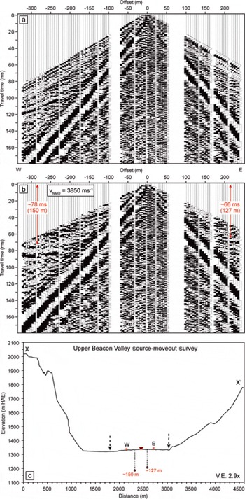
The common-offset plot shows a reflected phase at ∼78 ms for shots west of the spread and ∼66 ms for shots east of the spread (Fig. 10a). These reflections are observed for shot offsets >150 m, where they arrive before the high-amplitude ground roll. After NMO correction, depth estimates for these reflected arrivals are ∼150 m for shots west of the spread and 125–130 m for shots east of the spread (Fig. 10b). We interpret this deep reflection as the valley floor beneath a continuous layer of ice containing scattered debris. These depths are consistent with extrapolations of the eastern valley wall beneath the survey site (Fig. 10c).
Internal structure
In addition to ice-thickness estimates, the GPR and seismic data provide new information about the internal structure and composition of Mullins Glacier. This information is critical for understanding glacier dynamics, Mullins till development and surface ridge formation.
Hyberbolic diffractions
The GPR data and surface excavations in upper Mullins Valley show that the ice appears relatively clean when compared with buried ice in central Beacon Valley (e.g. Reference SugdenSugden and others, 1995; Reference MarchantMarchant and others, 2002) and debris-covered glaciers elsewhere (e.g. Reference Wahrhaftig and CoxWahrhaftig and Cox, 1959; Reference Potter, Steig, Clark, Speece, Clark and UpdikePotter and others, 1998). Well-defined hyperbolic diffractions are observed over a range of depths in the unmigrated GPR data (Fig. 6a); these diffractions appear as point scatterers or short linear features in the migrated profiles (Figs 4, 5 and 7). More of these diffractions are observed at shallower depths, but this may be attributed to the weaker signal return strength for greater depths. We conclude that the diffractions most likely represent individual cobbles/boulders or localized collections of debris within the ice.
Continuous internal reflections
Perhaps the most interesting result of the GPR and seismic surveys in upper Mullins Valley is the documentation of englacial dipping reflectors. The most noteworthy internal reflector spans nearly the entire thickness of Mullins Glacier at the first ridge site (Fig. 5). The GPR profiles show that this reflector displays a steep up-valley dip (40–45°), with a surface intersection at the first large ridge on Mullins Glacier (Fig. 5). Farther up-valley, the reflector undulates with dips ≤10° at depths of 60–80 m, only 10–15 m above the interface interpreted as the valley floor. The transverse profile shows that this interface has a slightly asymmetric, concave-upward cross-section with three-dimensional (3-D) geometry similar to that of an up-valley plunging syncline (Figs 5 and 11).
Fence-post diagram for GPR profiles in upper Mullins Valley showing location and 3-D geometry of reflectors (Fig. 2b for view orientation).

Reflections from this interface are also observed in the seismic data (Fig. 8). Analysis of individual shot gathers shows a shallow phase with non-traditional moveout for source locations up-valley of the first ridge (Fig. 8a and b); receivers down-valley of the ridge do not show this shallow phase, regardless of shot location. The shallow arrivals that appear linear in individual shot gathers display NMO in CMP gathers with v NMO of 5000–5300 m s−1, which is consistent with the expected apparent NMO velocity for reflections arising from a 40–45° dipping interface within a layer of ice (apparent v NMO = v ICE/cos(dip)).
To confirm that the shallow reflections are related to the same dipping interface observed in the GPR data, we generated a synthetic seismic dataset using a simple subsurface model derived from the longitudinal GPR profile. A triangulated sloth (1/velocity2) model was created for an ice layer with a velocity of 3760 m s−1 above a layer representing the valley floor (4100 m s−1). A 25 cm thick layer with velocity of 3950 m s−1 was defined within the ice layer to represent the internal dipping reflector. Synthetic shot gathers were generated (Fig. 8c and d), and the results confirm that the shallow reflections observed in the field data are indeed produced by the englacial layer. The synthetic data show that for certain acquisition geometries, the steeply dipping reflector produces two arrivals (Fig. 8c and d): a more traditional hyperbolic reflection associated with the deeper, sub-horizontal portion of the layer and a more linear reflection with higher apparent velocities, associated with the steeply dipping, shallow portion of the layer. The field data clearly show reflections from the steep, near-surface portions of the englacial interface, but most shot gathers lack the coherent reflections expected from the sub-horizontal, deeper portions farther up-valley (Fig. 8a and b). This may be related to signal attenuation or variations in the continuity and/or material properties of the englacial layer. We favor the latter, which implies that the steeply dipping portions of the englacial layer display greater continuity and/or a higher concentration of non-ice component(s). This interpretation is consistent with observations of the return signal strength in the longitudinal GPR profile, with much stronger returns observed for the shallower, down-valley portions of the englacial layer (distances of 110–240 m in Fig. 5a).
The steep dip of this englacial interface complicates seismic data processing. Several attempts to apply pre-stack dip moveout corrections to the data-using techniques specified by Reference Yilmaz and DohertyYilmaz and Doherty (2001) were unsuccessful. Due to these complications, the CMP stack presented in Figure 9 does not include the shallow reflection. Consequently, the most accurate representation of the englacial interface comes from the migrated GPR data along the same survey line (Fig. 5a).
Close examination of the near-surface longitudinal GPR profile at the first ridge site (Fig. 6a; distances of 200–240 m in Fig. 5a) shows that the steeply dipping englacial reflection consists of at least three individual reflectors with a separation of ∼2 m (Fig. 6a and b). The available data do not show this same substructure at depths greater than ∼25 m, suggesting that either the data quality at depth is insufficient to resolve these individual reflections or the dipping reflector is splayed/bifurcated only near the surface. One of these individual reflectors intersects the surface on the up-valley slope of the first ridge, while another appears to intersect the surface closer to the ridge crest. Analysis of the transverse GPR profile at the first ridge site shows that the western surface intersection of the dipping internal reflection (Fig. 5c profile origin) is located at the ridge crest, while the eastern intersection is located on the up-valley ridge flank (Fig. 5c).
In addition to the englacial reflectors at the first ridge site, we also observe englacial reflectors at the exposed ice site and the second ridge site. At the exposed ice site (near the valley headwall), the longitudinal GPR profile shows what appear to be linear reflections with an up-valley dip spanning depths of 20–40 m (Fig. 4a). The reflectors are generally located beneath two long-wavelength surface undulations (distances of 200–430 m from the profile origin in Fig. 4a), but a relationship between these englacial reflectors and the long-wavelength surface features cannot be established based on the available data.
An englacial reflector is also observed near the valley floor at the second ridge site (Fig. 7), although the data are not as robust as those from the first ridge site. While no reflectors appear to intersect the ice surface at the second ridge site, the available data suggest that the deep englacial interface could intersect the surface farther down-valley.
Interpretation of continuous internal reflections
From a physical standpoint, the reflectors must involve a significant contrast in material properties to produce the observed reflections in both the GPR and seismic data. This material contrast could potentially arise from changes in ice (1) purity (debris concentration), (2) temperature (e.g. Reference KohnenKohnen, 1974; Reference Maijala, Moore, Hjelt, Pälli, Sinisalo and PlumbMaijala and others, 1998), (3) fabric or crystal orientation (e.g. Reference HarrisonHarrison, 1973; Reference Blankenship and BentleyBlankenship and Bentley, 1987; Reference HorganHorgan and others, 2008), (4) density (bubble content) or (5) some combination of these factors.
Based on the observed ice thicknesses and the magnitude of the return strength for the internal dipping reflections, we dismiss explanations involving temperature, fabric and/or density variations. Both the seismic and GPR data show that reflections from this interface display a negative–positive–negative polarity, suggesting the presence of a material with increased acoustic impedance (product of seismic velocity and material density) and relative dielectric permittivity. This polarity is consistent with that of GPR reflections from the layer of dolerite cobbles at the base of the frozen meltwater pond (Fig. 6). Taken together, these observations suggest that the inclined reflectors, even at depth, arise from an englacial debris band(s) containing dolerite clasts.
To follow up on the GPR survey results, we excavated a ∼5 m long, ∼60 cm deep and ∼50 cm wide longitudinal trench on the up-valley side of the ridge (Fig. 12). This excavation through the debris cover and into glacier ice revealed five debris bands separated by clean, bubbly ice. The englacial debris bands are, for the most part, comprised of isolated clasts, with very little intervening matrix sediment. Exceptions occur alongside the largest clasts, which tend to rest directly on scattered and weathered pea-sized gravel. This situation is similar to that observed on the surface of Mullins Glacier near the valley headwall (up-valley of the frozen meltwater pond), where many isolated cobbles rest, in whole or in part, on a thin layer of weathered gravel. Of the 11 englacial clasts removed from the bands, none showed evidence for glacial abrasion (e.g. no striations, molding or polish), and the a axis of all clasts dipped at up-valley angles ≥30° (i.e. parallel to the overall dip of the debris bands and greater than or equal to the ridge surface slope).
(a, b) Surface exposure and trench excavated across the first large ridge. A package of sub-parallel debris bands can be seen intersecting the surface near the ridge crest, with some embedded clasts >30 cm across. Measuring tape is 50 cm long. (c, d) View of the exposure/trench looking east along the ridge crest. Thick dashed curves delineate ridge microtopography and variations in the debris cover associated with the englacial debris bands.

Small steps and/or ridges occur along the main ridge crest wherever individual debris bands intersect the surface (Fig. 12c). The small ridges produce a stepped profile along the up-valley flank of ridge, with each step being demonstrably related to the location and texture of underlying englacial debris layers.
The Mullins till that caps the ridge crest is nearly identical to underlying englacial debris, with two minor differences: (1) clasts at the surface of Mullins till show slightly greater levels of surface staining than observed on englacial clasts, and (2) Mullins till contains a greater proportion of (windblown?) sand and fine-grained gravel than observed in englacial layers. All other physical attributes, including clast size, lithology (predominantly Ferrar dolerite) and shape (angular to sub-angular), are virtually identical.
Extraction of shallow ice cores along the ridge crest met refusal at ≤2.5 m, presumably where the core head encountered englacial debris. Cores collected at distances of tens to hundreds of meters both up- and down-valley from the first ridge easily penetrated to depths of 10 to >25 m without encountering significant englacial debris.
Discussion
Source for englacial debris bands
The ultimate source for englacial debris is either subglacial or supraglacial, and entrainment can occur through either passive or active processes (Reference Alley, Cuffey, Evenson, Strasser, Lawson and LarsonAlley and others, 1997; Reference KnightKnight, 1997). The most likely debris source/entrainment pairs for Mullins Glacier are: (1) a subglacial source with active entrainment through shearing/thrusting or (2) a supraglacial source involving rockfall with passive entrainment as primary stratification.
In favor of a subglacial source is the observation that the internal dipping reflector at the first ridge site appears to originate near the reflection interpreted as the valley floor (Fig. 5a). Furthermore, the longitudinal GPR data from the first ridge site suggest that an additional interface may be present between the valley floor reflection and the internal dipping reflector (distances of 0–100 m in Fig. 5a and b). This additional reflection could potentially represent a layer between relatively clean glacier ice and the valley floor that could serve as a source for subglacial debris entrainment at this location. Entrainment of this subglacial debris could potentially occur along a shear zone/thrust fault (e.g. Reference Chinn and DillonChinn and Dillon, 1987; Reference Clarke and BlakeClarke and Blake, 1991; Reference Hambrey, Dowdeswell, Murray and PorterHambrey and others, 1996, Reference Hambrey, Bennett, Dowdeswell, Glasser and Huddart1999; Reference Murray, Gooch and StuartMurray and others, 1997; Reference Fukui, Sone, Strelin, Torielli, Mori and FujiiFukui and others, 2008), within basal crevasses (Reference SharpSharp, 1985; Reference Ensminger, Alley, Evenson, Lawson and LarsonEnsminger and others, 2001; Reference Woodward, Murray, Clark and StuartWoodward and others, 2003) or through the folding of basal ice or subglacial debris layers (e.g. Reference Glasser, Hambrey, Crawford, Bennett and HuddartGlasser and others, 1998).
Debris bands displaying a steep up-glacier dip have been documented within debris-covered glaciers on James Ross Island, Antarctica (Reference Chinn and DillonChinn and Dillon, 1987; Reference Fukui, Sone, Strelin, Torielli, Mori and FujiiFukui and others, 2008), and near the margins of surge-type glaciers in Svalbard (Reference Bennett, Hambrey, Huddart and GhienneBennett and others, 1996a,Reference Bennett, Huddart, Hambrey and Ghienneb; Reference Hambrey, Dowdeswell, Murray and PorterHambrey and others, 1996, Reference Hambrey, Bennett, Dowdeswell, Glasser and Huddart1999; Reference Murray, Gooch and StuartMurray and others, 1997; Reference Woodward, Murray and McCaigWoodward and others, 2002, Reference Woodward, Murray, Clark and Stuart2003), in western Yukon, Canada (Reference Clarke and BlakeClarke and Blake, 1991), and in Sweden (e.g. Storglaciären; Reference Jansson, Näslund, Pettersson, Richardson-Näslund and HolmlundJansson and others, 2000). Most of these studies conclude that the en-glacial debris bands were formed due to active entrainment of basal debris along thrust planes or within shear zones. However, it is important to note that these studies involved polythermal, warm-based or surge-type glaciers, and their relevance to the cold-based Mullins Glacier is limited.
Given the present thermal conditions and minimal surface displacement rates (Reference Rignot, Hallet and FountainRignot and others, 2002), we suggest that direct basal entrainment is unlikely for Mullins Glacier. In reaching this conclusion, we considered several recent studies that suggest some cold-based glaciers may actively modify their beds and entrain debris (Reference Tison, Petit, Barnola and MahaneyTison and others, 1993; Reference CuffeyCuffey and others, 2000; Reference Atkins, Barrett and HicockAtkins and others, 2002). While these studies provide an intriguing perspective, the examples provided and mechanisms proposed for debris entrainment in basal ice seem incapable of producing the relatively thick, continuous debris layers containing large cobbles/boulders observed within Mullins Glacier. Furthermore, clasts examined in englacial layers show no evidence for subglacial modification such as striations, faceting or evidence of comminution as might be associated with subglacial entrainment (e.g. Reference BoultonBoulton, 1970, Reference Boulton1978).
Our favored origin for the observed englacial debris layers involves a supraglacial source (rockfall) followed by passive entrainment beneath younger snow and ice. In this model, clasts from minor rockfall events that come to rest in the accumulation zone are subsequently buried by snow/ice, eventually traveling englacially with ice flow. Flow in the accumulation zone can transport supraglacial debris very close to the bed (Reference Alley, Cuffey, Evenson, Strasser, Lawson and LarsonAlley and others, 1997), with originally surface-parallel layers developing a characteristic up-valley dip (Reference PatersonPaterson, 1994), reflecting cumulative shear; debris-rich layers with a similar up-valley dip are commonly associated with primary stratification in alpine glaciers (e.g. Reference Benn and EvansBenn and Evans, 1998).
Alternatively, the englacial layers may form during periods of net negative mass balance and ice loss in the accumulation zone. In this scenario, scattered englacial clasts are brought to the ice surface through ablation of the overlying ice, producing a surface lag much like modern Mullins till (with or without additional rockfall input). A return to positive mass balance would bury the lag with additional snow/ice, which would then flow englacially just as for the case described above.
Surface ridge formation/modification
While a direct correlation between englacial debris bands and all surface ridges may not exist for Mullins Glacier (based on available data), a relationship between the first large ridge and the underlying englacial debris band is apparent. Accordingly, it is tempting to link englacial debris bands with the formation of surface morphology. For example, we surmise that local surface lags would form wherever dipping englacial debris bands intersect the surface of otherwise relatively clean glacier ice. These local surface lags would, in turn, modify subsequent loss of underlying ice (e.g. Reference Kowalewski, Marchant, Levy and HeadKowalewski and others, 2006), resulting in localized differential ablation. Over time, this differential ablation and subsequent gravitational redistribution of debris could contribute to the development of asymmetric surface ridges. Sub-parallel debris bands, like those identified in excavations at the first ridge site, could also produce smaller micro-ridges through this process (Fig. 12). Supraglacial-ridge formation/modification via differential ablation has been documented for a range of glacial environments (e.g. Reference Rains and ShawRains and Shaw, 1981; Reference Bennett, Huddart, Hambrey and GhienneBennett and others, 1996b; Reference Lyså and LønneLyså and Lønne, 2001).
Although there is no direct evidence for localized strain in ice beneath surface ridges, we cannot preclude thrusting as an additional mechanism for surface ridge formation and/or modification. Reference NyeNye (1951), for example, noted that the development of thrust planes may be localized at thrust ‘breeding grounds’ in alpine glaciers. At these locations, increased compressive stresses can result in displacement along slip lines (typically with a ∼45° surface intersection angle) and/or along existing planes of weakness (e.g. englacial debris bands, laminations, foliation) in a favorable orientation (Reference IvesIves, 1940; Reference NyeNye, 1951). As the ice moves down-valley, these thrust planes become inactive and are preserved within the ice, while new thrust planes are formed at the ‘breeding ground’. Depending on displacement rates and magnitude, this thrusting could result in surface disruption in the form of asymmetric surface ridges. Near-surface splaying along sub-parallel thrusts might also be expected, potentially explaining the individual debris bands and microtopography associated with the first large ridge on Mullins Glacier.
In this scenario, the first large ridge represents the surface manifestation of the most recent thrust to form within Mullins Glacier, and the down-valley ridges may represent the surface intersections of inactive thrust planes. Subsequent modification of surface ridges associated with inactive thrusts would result in decreased relief, lower slopes and a more rounded cross-sectional profile, as is observed for down-valley ridges in lidar topography (Fig. 1) and field studies for Mullins Glacier. It is also possible that thrusts could be reactivated at favorable down-valley locations, like the corridor where Mullins Glacier enters upper Beacon Valley.
Evaluating previous flow models
The valley floor reflection observed in the CMP stack and GPR profiles shows no indication of the bedrock depression and increased ice thicknesses predicted by the flow models of Reference Rignot, Hallet and FountainRignot and others (2002) and Reference Shean, Head and MarchantShean and others (2007b). Since the surface slopes used for the models are well constrained, this discrepancy could be related to (1) errors in the InSAR surface displacement data at these locations (potentially arising from insufficient surface debris to reflect the 5.3 GHz SAR waves), (2) vertical surface displacements unrelated to flow during the period of the InSAR measurements (e.g. unusually rapid ablation, additional meltwater freezing onto surfaces up-valley of the first large ridge) and/or (3) thrusting near the first ridge site, resulting in surface displacements that violate continuity assumptions made during horizontal velocity derivation and flow modeling. Future flow-modeling exercises using the valley-floor profiles presented here will provide a better framework for evaluating the existing surface velocity data.
Implications for environmental change
Similarities in morphology and relative spacing for ridges on Mullins and Friedman Glaciers suggest that their formation is related to changes in environmental conditions, including changes in mass balance and/or rates of rockfall deposition. Given uncertainties associated with rockfall deposition in ice accumulation zones (which involve changes in the size and geometry of accumulation zones, as well as non-linear effects of long-term bedrock weathering (e.g. Reference AckertAckert, 1998)), it is difficult to point to a single environmental factor that can be linked unambiguously to rockfall development. For example, periods of enhanced seismic activity could result in synchronous rockfall activity across valleys. Even with these considerations in mind, if we assume relatively constant rockfall rates in the recent past, changes in climate conditions are required to concentrate the surface debris necessary to form the observed englacial layers and/or enable thrusting. Whatever their precise origins, the sporadic englacial layers in Mullins Glacier, and presumably in Friedman Glacier, seem to suggest that regional geomorphic processes and environmental conditions have varied over time. Future analysis of ice cores/samples may provide an improved understanding of the magnitude of these environmental changes and their role in surface ridge formation and englacial debris entrainment.
Conclusions
The GPR and seismic surveys for Mullins Glacier provide ice-thickness estimates of 80–110 m near the valley headwall and >150 m in upper Beacon Valley. The data also reveal a stepped, concave-upward cross-sectional valley profile and a smooth, sub-horizontal bed profile along the glacier center line in upper Mullins Valley, with no evidence for an overdeepened bedrock basin as predicted in previous studies (Reference Shean, Head and MarchantShean and others, 2007b).
The surveys also reveal englacial debris as scattered cobbles/boulders and as discrete layers. The most extensive englacial layer originates just above the bed in upper Mullins Glacier and appears as a coherent reflector with a notable 40–45° up-valley dip. The debris layer intersects the glacier surface near the crest of an ∼8 m high ice-cored ridge, the largest and farthest up-valley of several ice-cored ridges that mark the glacier surface. The englacial layers most probably originate as (1) concentrated rockfall in the accumulation zone and/or (2) surface lags that form in the accumulation zone as dirty ice sublimes; the latter would require a period of extended negative mass balance and equilibrium-line altitude variation.
Although our results indicate that not all surface ridges on Mullins Glacier are associated with dipping englacial debris layers, the association of the largest ridge on Mullins Glacier with a package of sub-parallel dipping englacial debris bands suggests that the englacial layers likely play a significant role in the formation/evolution of at least some surface ridges. Though there is no direct evidence for localized strain in the ice beneath surface ridges, localized thrusting along englacial debris bands may also play a role in ridge formation/evolution. The similar morphology and relative spacing of ridges on Mullins and Friedman Glaciers suggests that ridge formation is likely related to regional environmental change.
These results provide constraints for evaluating mechanisms of debris entrainment and surface ridge formation for debris-covered glaciers on both the Earth and Mars. Mullins Glacier can serve as an analog for tongue-shaped or lobate features on Mars that display arcuate surface ridges and glacier-like morphologies suggestive of flow (e.g. Reference HeadHead and others, 2005; Reference Shean, Head and MarchantShean and others, 2005, Reference Shean, Head, Fastook and Marchant2007a; Reference Milkovich, Head and MarchantMilkovich and others, 2006; Reference Marchant and HeadMarchant and Head, 2007). These features may share similar internal structure and comparable surface ridge formation/modification mechanisms. An understanding of the morphological indicators of past environmental conditions in Mullins Valley (e.g. surface ridges, variations in debris cover) may improve interpretations of similar features on Mars that can provide new, indirect information about past climates on Mars.
Acknowledgements
We thank T. Parker and the staff at the PASSCAL Instrument Center for assistance with survey planning, equipment acquisition and field support, T. Nylen and UNAVCO for GPS survey support, S. Arcone for advice on GPR data processing, P. Morin for assistance with data visualization, and D. Kowalewski, J. Green, J. Dickson, G. Morgan, J. Levy, K. Swanger, J. Head and L. Robinson for assistance with data collection. We thank E. King and A. Fountain for insightful comments and constructive reviews. The multichannel seismic instruments used in the field were provided by the PASSCAL facility of the Incorporated Research Institutions for Seismology (IRIS) through the PASSCAL Instrument Center at New Mexico Tech. Data collected during this experiment will be available through the IRIS Data Management Center. The facilities of the IRIS Consortium are supported by the US National Science Foundation (NSF) under Cooperative Agreement EAR-0004370 and by the US Department of Energy National Nuclear Security Administration. This work was sponsored by NSF grant ANT-0338291 and ANT-0636705 to D.R.M., which is gratefully acknowledged.


