


1. Introduction
Between 1992 and 2018, the Greenland ice sheet lost enough mass to raise global sea level by 10.8 ± 0.9 mm (Shepherd and others, Reference Shepherd2020). As global warming continues to accelerate, increased melting of the ice sheets and – as a corollary – rising global sea levels, are expected to continue. Of particular concern is that just this past decade has seen the two highest melt years on record – in 2012 and 2019. In fact in July 2012, almost the entire ice sheet surface exhibited melting (Nghiem and others, Reference Nghiem2012). As such, it is increasingly important that we are able to monitor ice sheet surface melting with a high degree of fidelity, if we are to understand the current contribution of the Greenland ice sheet to global sea level rise and to constrain future predictions. To monitor melting at the ice sheet scale, microwave and optical remote sensing is often employed (e.g. Ashcraft and Long, Reference Ashcraft and Long2006; Fettweis and others, Reference Fettweis, Tedesco, van den Broeke and Ettema2011). Optical remote sensing is most often use to map melt features visible to the eye, e.g. supraglacial lakes and streams (Vandecrux and others, Reference Vandecrux2022). Microwave remote sensing includes the use of passive sensors including the Special Sensor Microwave/Imager (SSM/I) (Abdalati and Steffen, Reference Abdalati and Steffen2001) and active sensors including the advanced scatterometer (Colbeck, Reference Colbeck1982). Current methods to identify melting in data acquired by these sensors exploit the fact that the presence of liquid water changes the dielectric properties of snow and ice, and thus its signature in brightness temperature and backscatter images (Colbeck, Reference Colbeck1982). In fact, as little as 3% water content in snow can have a large enough impact on these properties for the difference to be discernible in microwave imagery (Golden and others, Reference Golden1998). Several methods have been proposed to classify image pixels in synthetic aperture radar (SAR) imagery into melting and nonmelting based on brightness temperature (with thresholding based on optical data Miles and others, Reference Miles, Willis, Benedek, Williamson and Tedesco2017), and backscatter values (interpreted using simple physical models or binary thresholding techniques McFeeters, Reference McFeeters1996). Recent advances have been made in a variety of surface ice/snow-related applications. Rotschky and others (Reference Rotschky, Rack, Dierking and Oerter2006) found that SAR data can be used to map mass-balance changes for certain snow pack regimes, retrieving snowpack properties, within a limited area. Liang and others (Reference Liang2021) used Sentinel-1 SAR images for detecting snowmelt over the Antarctic, focusing on assessing surface material loss and albedo change. Winsvold and others (Reference Winsvold2018) also used SAR satellite data, but for mapping glaciers in Norway, correlating SAR with optical images (Landsat 8) and additional data from local meteorological stations. Schröder and others (Reference Schröder, Neckel, Zindler and Humbert2020) studied the surface condition using SAR ground range detected product for differentiating liquid water from other surface conditions for better recognition of lakes. We note that current studies focus on certain surface types and certain melt stages, identifying only melt on ice/snow or identifying only lakes through the presence of liquid water. We explore further stages of melting for more surface conditions, including ice, snow and lakes.
Here, we use an advanced statistical method known as state-space modelling as the backbone to a data-driven classification system that can capture the state-switching process of the ice sheet pixels throughout both melt and nonmelt seasons. The use of Sentinel-1 SAR offers two main advantages over other sensors: (1) as an active sensor, SAR is largely insensitive to weather and can penetrate cloud cover (Nagler and others, Reference Nagler, Rott, Ripper, Bippus and Hetzenecker2016; Winsvold and others, Reference Winsvold2018) and (2) backscatter values comprise both a surface and a subsurface backscattering components (Fahnestock and others, Reference Fahnestock, Bindschadler, Kwok and Jezek1993), thus potentially providing information as to the underlying ice surface type (ice, snow and open water) as well as surface melting state. In developing our classification system, we use optical images (Landsat 8) to help identify the surface types and the regional climate model MAR (Modèle Atmosphérique Régional) (Franco and others, Reference Franco, Fettweis and Erpicum2013) to interpret the state-switching estimates. Since the melting process differs across the surface types, the two classifications can help to reinforce each other. Current methods using thresholding technique or other modelling technique focus on identifying either melt (for ice/snow) or liquid water (for lake). Our approach automatically partitions SAR backscatter data into snow, dark ice and ice/lake pixels, and assigns a melting, nonmelting or transit state to each pixel. Our method thus provides a comprehensive representation of the entire process and requires no prior knowledge of surface conditions (ice, snow and lakes). In Section 2, we provide the background of the study area and describe the main auxiliary data; in Section 3, we explain the method developed based on nine selected sites, covering three scenarios, for recognising the state-switching process on the ice sheet surface; in Section 4, we present testing results at unseen locations on the ice sheet. Section 5 provides a conclusion to this work.
2. Study area and data
2.1. Study area
We focus on a northeast sector of the Greenland ice sheet covering Nioghalvfjerdsbræ, or 79 N° glacier (79 N°) and Zachariae Isstrøm (ZI) (Fig. 1). The 79 N° glacier has a floating ice tongue extending 70 km into 79 N° fjord and has thinned by 30% since 1999 (Lindeman and others, Reference Lindeman2020). ZI covers a region 100 km from north to south and up to 50 km from east to west. Together, 79 N° and ZI comprise the end of the northeast Greenland Ice Stream, which drains about 12% of the interior of the ice sheet (Davies and others, Reference Davies2022). Evaluating surface melt in this region is of particular interest for several reasons. The Greenland Ice Sheet now contributes over 25% of observed global sea level rise (Ryan and others, Reference Ryan2019) and has become the single largest contributor to sea level rise (Velicogna and others, Reference Velicogna, Sutterley and van den Broeke2014). Mass loss in this northeast sector is accelerating (Zwally and others, Reference Zwally2002). The estimated runoff was 357 ± 58 Gt yr−1 on average during a 9-year period prior to 2020 (Slater and others, Reference Slater2021). It is also now thought to be the region of the ice sheet undergoing the greatest inland expansion of supraglacial lakes (Ignéczi and others, Reference Ignéczi2016; Turton and others, Reference Turton, Hochreuther, Reimann and Blau2021). This suggests that this region is experiencing large changes in melting (Selmes and others, Reference Selmes, Murray and James2011), and is ideal as a study area to investigate ice sheet surface melt.
(a) Greenland ice sheet. Left panel box on the northeast shows a backscatter image of the target area, and right panel shows the map with the snowline determined by ESA using Sentinel-3 data in 2021 (https://www.esa.int/ESȦMultimedia/Images/2022/05/Greenlanḋsnowlinėretreaṫanḋrainfall). (b) A SAR image of the northeast Greenland with prelabelled sites. (c) A Landsat optical image acquired 2017-07-30; the shaded region is the SAR image overlaid.
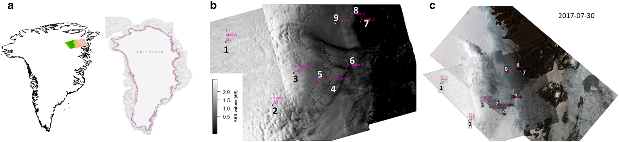
To build an automatic classification system, we select nine separate point locations from across the study area, covering ice, snow and lake surfaces, for use as training sites. The sites were selected to cover a range of surface types based on their appearance in a Landsat-8 image acquired in 2019. Three points below the snow line were chosen (sites 7–9), on the assumption that they represent the ice surface, three points above the snow line were chosen on the assumption that they represent the snow surface (sites 1–3), where site 1 is the furthest inland and site 3 is the closest to the snowline, and three points were chosen from within supraglacial lakes, visible as open water in the Landsat image (sites 4–6).
Of the supraglacial lake sites, site 4 is a large lake that appears to remain frozen in some summers, when cross referenced with optical satellite imagery. Site 5 is a small lake in the percolation zone of the ice sheet that appears to freeze over and is snow covered each winter. Site 6 is also a small lake, but located closer to the ice margin. This lake also appears to freeze over and become snow covered in winter. Of the ice sites, two points are located on clean ice and one point (site 7) is located in the dark ice zone that appears each summer on Greenland. The ice here is characterised by high amounts of embedded debris, and is also thinner than the clean ice upstream.
2.2. Sentinel-1 SAR backscatter data
Here, we use single look complex SAR backscatter data acquired from Sentinel-1 between December 2015 and May 2020. The 2-satellite constellation, Sentinel-1a and Sentinel-1b satellites, provides data every 6 days. Sentinel-1 SAR has a central frequency of 5.405 GHz and the pixel spacing of the backscatter image is 46.5 × 55.5 m. We re-sample the SAR images at a regular grid, and the spatial resolution is 6 × 6 km after re-sampling. Preprocessing has been applied to the dataset following the ESA protocol, including speckle reduction, geocoding, noise filtering and coregistration.
The SAR pixel values range from 0 to 1.5 dB, which is a logarithmic unit. Since the distribution of the SAR data points appears to be left truncated at 0, the assumption of a normal distribution in our following state-space model would otherwise be inappropriate. Thus, we apply a log-normal transformation to the SAR data. State-space models with normal error distributions are then fitted to these data. We note that the log-transformation is often used in statistics to combat this truncation issue.
2.3. Climate data
To establish a link between surface melt behaviour and SAR backscatter variations, we mainly use total daily snowfall, total daily meltwater production, daily surface mass balance (SMB) and daily rainfall simulated by the MARv3.11.5 regional climate model (Fettweis and others, Reference Fettweis2020) , run at a resolution of 6 km and 6 hourly forced by the ERA5 reanalysis at its lateral boundaries. MAR is a regional climate model that can be used for simulation from km-scale to continental-scale (Fettweis and others, Reference Fettweis2020). For each of the nine training sites, and all of the testing pixels in the 6 × 6 km grid, we extract a time series for each of these variables from the MAR data using the MAR grid cell with centre closest to the training/testing point location. A list of the training and testing site locations is given in Appendix A. Further MAR variables are explored and included in Appendix B.
3. Methods
Our method can be summarised as follows: (1) We extract time series data from SAR backscatter images at our nine training locations. (2) After log-transforming the data, we use a state-space model to partition each time series into a number of separate states, based purely on their statistical properties. (3) Through visual inspection of long-term optical images and with reference to the climate model output (Fettweis and others, Reference Fettweis2020), we characterise these states as being associated with ice, snow or open water, melting or nonmelting and with weather events such as rainfall and snowfall. (4) We use this analysis to develop a set of decision rules, by which unseen pixels can be classified according to their surface properties.
3.1. State-space model
State-space models have been widely used for analysing time series data (see Fahrmeir and Tutz, Reference Fahrmeir and Tutz2001 for an introduction). A state-space model relates responses to an unobserved state by a probabilistic model, and the states are assumed to follow a latent or hidden Markov model (HMM) (Fahrmeir and Tutz, Reference Fahrmeir and Tutz2001). The state-space model, also known as HMM, is fitted in the frequentist framework with no prior information (see Visser and Speekenbrink, Reference Visser and Speekenbrink2010 for an R package).
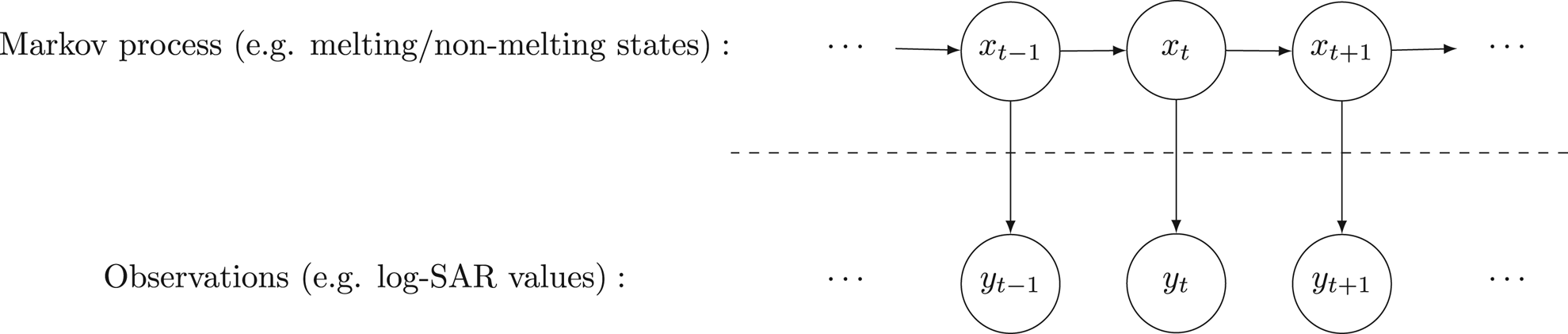
In a discrete-time state-space model, for time series data {y t}, e.g. log-SAR values, where t denotes the time at which the observation is taken. The latent, or hidden, model for the states {x t}, e.g. melt or nonmelt, follows a Markov process with a discrete state space. Figure 2 gives an illustration of a state-space model, which links the observations y t to a hidden or latent (unobserved) state process, x t.
A state-space model with an unobserved state process x t and an observation sequence y t. The dependence among the observations is generated by the states: y t is conditionally independent from all other variables given the state x t; and x t is conditionally independent from x 1, ⋅ ⋅ ⋅ , x t−2 given x t−1.
The purpose of fitting state-space models to time series SAR data is to discover the unobserved hidden states that explain the variations in the SAR measurements and decode the melting process over the ice sheet. The most-likely state sequence is recovered via the Viterbi algorithm (Forney, Reference Forney1973). The state process is assumed to be a Markov process, which means that the future and the past values are independent conditional on the present values, i.e. P (x t|x 1, ⋅ ⋅ ⋅ , x t−1) = P (x t|x t−1). The observations y t are assumed to be independent of one another given the states x t and the observations at time t are distributed as $Y_t\vert X_t = x_{t} \sim {\cal N}( \mu ,\; \Sigma )$ , where μ and Σ represent the mean and co-variance of a normal distribution, respectively. The main motivation for using state-space models is that the distribution of the observations at time t are specified by the value of the hidden state at time t.
In the context of modelling SAR data, our state-space model is specified by the set of states S = {s 1, s 2, ⋅ ⋅ ⋅ , s N}, corresponding to the possible ice sheet surface melt conditions, and a set of model parameters Θ = {π, A, B}, given a hidden state sequence X t = {x 1, x 2, ⋅ ⋅ ⋅ , x t}, x t ∈ S, and the observation sequence Y t = {y 1, y 2, ⋅ ⋅ ⋅ , y t}, the log-SAR values. The initial state probability π i = P(x 1 = s i), $\hbox {for} \ i = 1,\; \ldots ,\; N$ denotes the probability of the first observation being in state s i. The transition probabilities, a ij in matrix A, are the probabilities of hidden state i transitioning to state j, i.e. a ij = P(x t = s j|x t−1 = s i). The emission probabilities b it, in matrix B, characterise the likelihood of an observation at time t, given a state s i, i.e. b it = P(y t|x t = s i). For each state s i, $b_{it} \sim {\cal N}( \mu _i,\; {\sigma _i}^2)$
 .
.
To build the state-space model, we must assume a maximum number of hidden states and the possible transitions among states. Given the sampling frequency of the observed data, it is reasonable to build an initial model that includes five stages. This is also reasonable from a glaciological perspective, since it is possible for a lake pixel to transition from dry snow to melting snow to melting ice to open water to dry ice. Since not all of these states will be observed in all locations, we build several state-space models, varying the total number of states, and select the best fitting number of states based on the properties of the time series SAR data. We obtain a sequence of discrete states x t = s i, s i ∈ {1, 2, 3, 4, 5}, five being the maximum best fitting number of states across the training sites, from the fitted state-space models. Further details about our state-space model can be found in Appendix C.
3.2. Site characteristic classification
The state-space model captures the temporal variation in the physical processes of ice sheet melt. To consider spatial variations, we sample pixels in different regions. For example, the top panel in Fig. 3 shows the temporal variation in ‘snow’ regions. We chose these three sites because they span the range of conditions experienced above the ‘snowline’ in Greenland. Site 1 is situated in the ‘dry snow zone’, where no melt generally occurs and sites 2 and 3 are situated in the upper and lower ‘percolation zone’, respectively, and so experience different amounts of melt. It was important to choose this range of sites to robustly test our method. The ‘lake’ and ‘ice’ sites are chosen similarly.
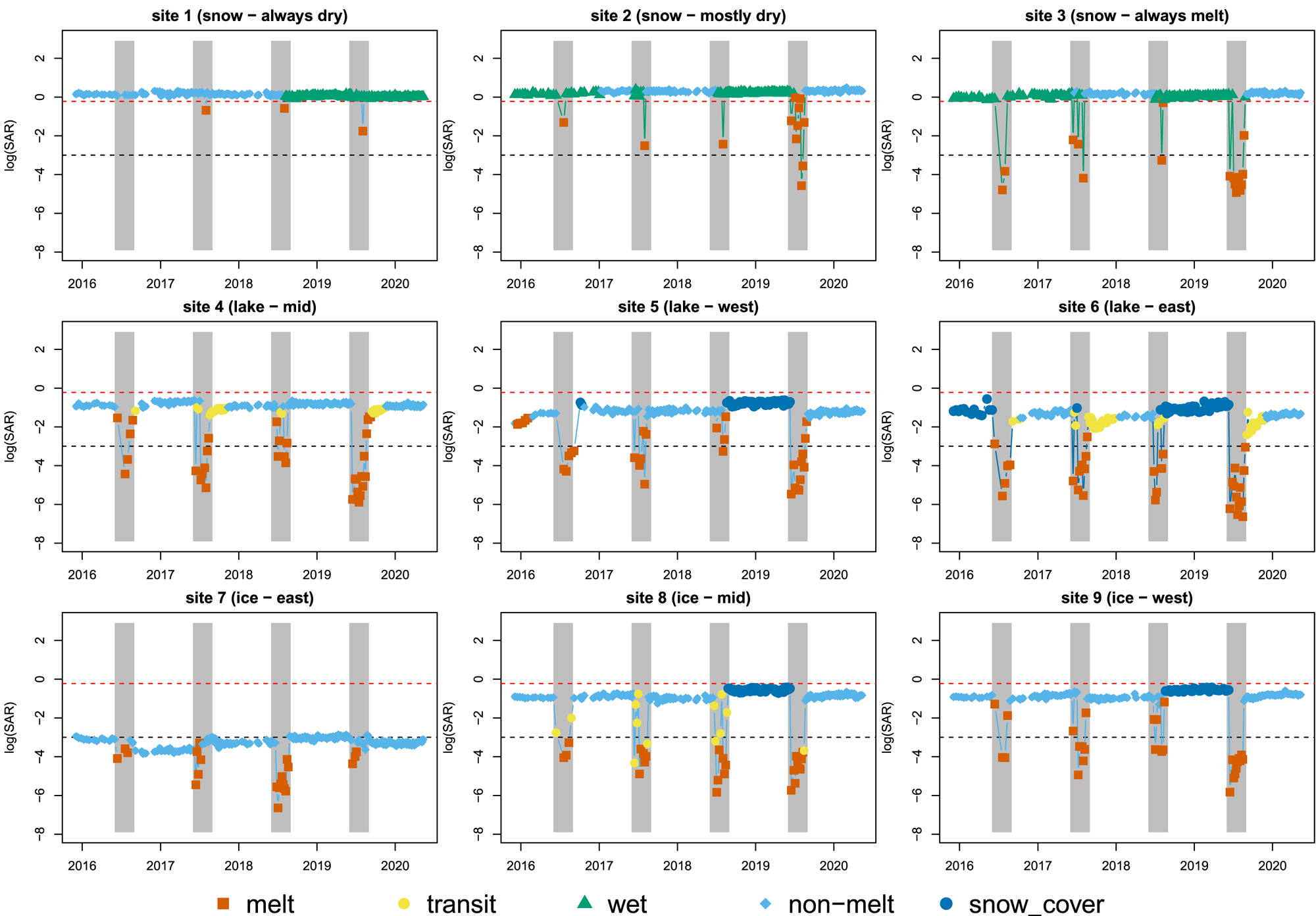
Time series of SAR backscatter values (log-scale) at nine study sites. States are represented by different colours and different number of states are recognised at each site. Most sites have a total number of 3 states. Site 8 has the highest number of 5 states. The orange states in each plot indicate the melt during summer, and the grey vertical shades highlight summer seasons. The two horizontal lines are the log(0.8) (red) and log(0.05) (black). During nonmelt season, snow sites (1–3) have values above the red dashed lines. Site 7 is a black ice site and has value lower than the black dashed line.
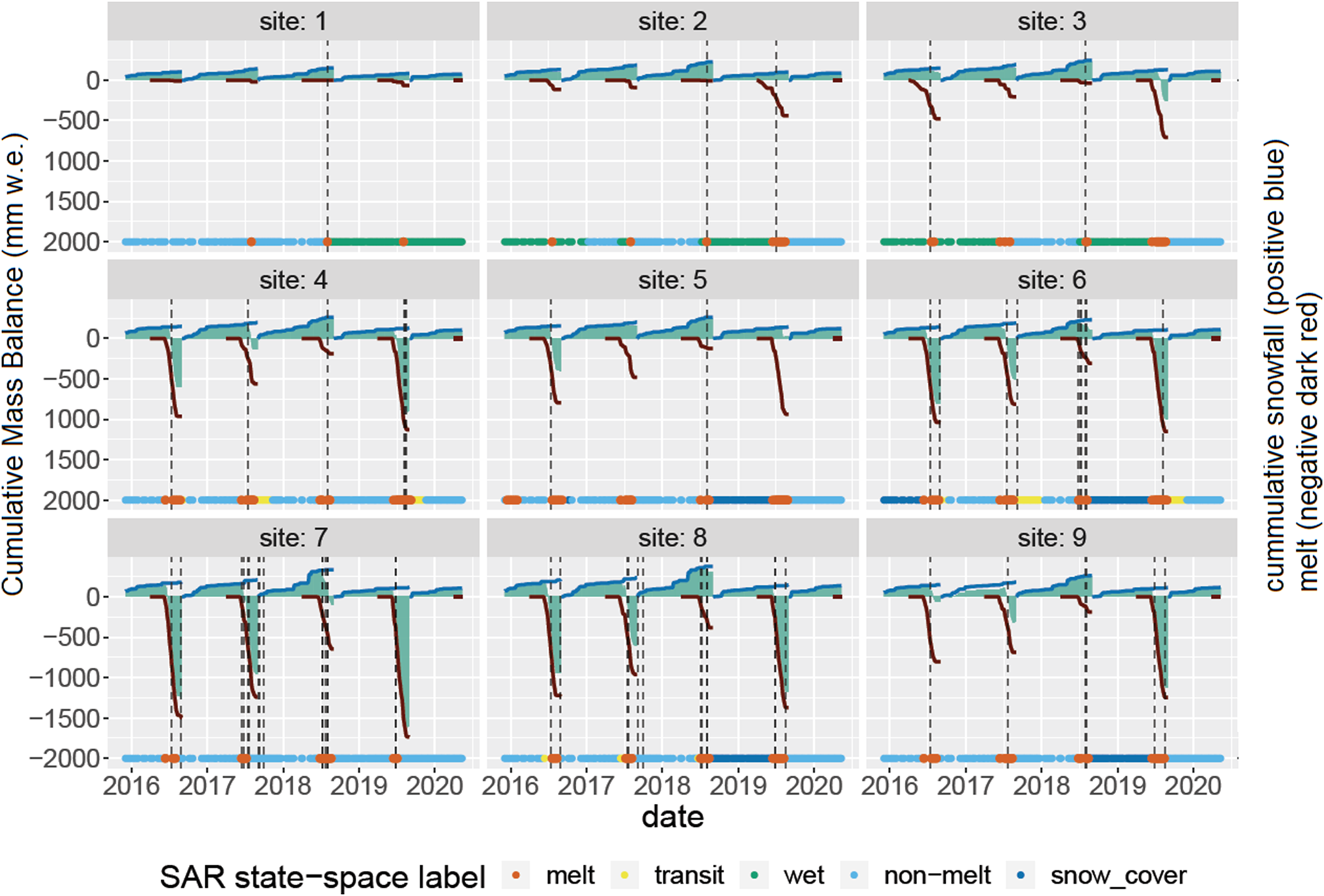
The next step is to relate the states to specific characteristics of the ice sheet surface. To do this, we examine temporal variability in our numbered states (Fig. 3) in combination with MAR climate model output (Fig. 4).
Comparison of the SAR states and the MAR climate model output. Positive blue lines: cumulative snowfall mm w.e. d−1; negative dark red lines: cumulative meltwater production mm w.e. d−1; light green bars: cumulative SMB mm w.e. d−1; dashed vertical lines: rainfall threshold above 1 mm w.e. d−1; coloured horizontal lines: SAR states from the fitted state-space models.
The nine sites exhibit three different backscatter modes, high (snow sites 1 − 3), low (snow sites 4 − 6 and 8 and 9) and very low (snow site 7), which is consistent with what would be expected from sites with different surface types (Nagler and others, Reference Nagler, Rott, Ripper, Bippus and Hetzenecker2016). Winter backscatter values at snow sites range from 0.8 to 1.4 dB and do not exceed 0.05 dB at site 7. Site 7 is located on the part of the Greenland ice sheet which is characterised by embedded dust and debris and thus appears dark both to the eye and to SAR (Humbert and others, Reference Humbert2020). The other five sites all exhibit winter mean backscatter values between 0.05 dB and 0.8 dB; we see no statistically significant difference between the other ice and lake sites.
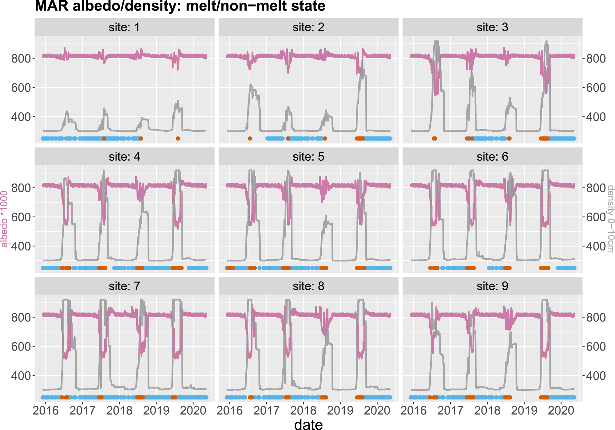
All nine sites exhibit a drop in backscatter values in the summer, with the lowest values in each year being picked up by our state-switching model as a distinct state. The presence of liquid water is known to lower the backscatter values on a glaciated surface (e.g. Golden and others, Reference Golden1998), and considering the time (summer) during which the state-switching occur, we assume that this state corresponds to surface melt. Our assumption is validated by comparing with temporal variation in melt (Fig. 4), albedo and surface density from MAR model (Fig. 9 and 10), which clearly show that these low-backscatter states occur when MAR predicts surface melting in summer.
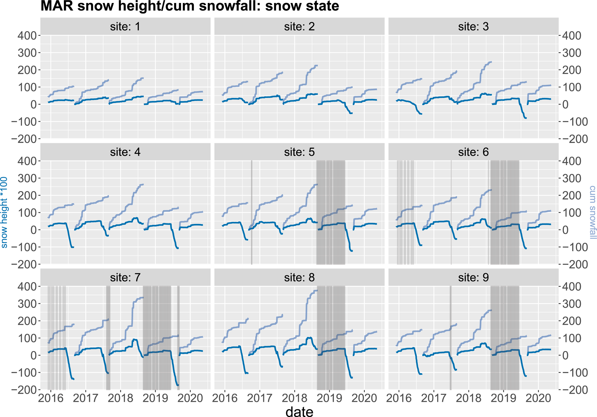
Winter backscatter at snow sites is partitioned into two states by our state-switching model (Fig. 3), with backscatter values that are slightly lower than the average winter (Dec–Jan–Feb) mean in some years, e.g. 2018/2019. If we cross reference with rainfall data from MAR, we can see that this lower backscatter state occurs after a nonnegligible rainfall event (i.e. rainfall above 1 mm w.e. d−1) and in the absence of significant snowfall. Rainfall on snow on Greenland is likely to alter the snow grain structure and refreeze between grains. This would increase the near-surface density of the snowpack and thus reduce SAR backscatter (Liu and others, Reference Liu, Wang and Jezek2006). An exception to this in our data appears to be at site 2 where rainfall in the summer of 2019/2020 does not result in lower backscatter the following winter. We hypothesise that this is because the rainfall event happened at the beginning of the melt season, and so any impact on the snow surface is likely to have been removed by subsequent melting. Two of the lake sites (5 and 6) and two of the ice sites (8 and 9) also exhibit winter backscatter values that take one of two states in our model, with the winter of 2018/2019 exhibiting a slightly higher mean backscatter than the winters before or since. Again, from cross-referencing with the regional climate model data (Fig. 4), we see this is likely because the summer of 2018 was characterised by lower melt and higher snowfall than usual. This would result in higher backscatter because volume scattering in snow (one of the components of the backscatter signal) increases with snow depth (Singh and others, Reference Singh2020). Figure 10 further illustrates that the snow cover states coincide with high accumulative snowfall and changes in snow height.
Our model predicts one additional state at two of the lake sites (4 and 6) and one of the ice sites (8). This occurs during the spring and autumn as the system transitions from nonmelting to melting, and back again. For the lakes sites 4 and 6, it is reasonable that this is predicted to be a distinct state since supraglacial lakes exhibit complex phase change behaviour; they freeze over in the autumn forming an ice lid which melts through in the spring (Law and others, Reference Law2020). The transitional states captured by our model therefore likely correspond to lakes freezing over in the autumn/winter and unfreezing in the spring/summer. It is interesting to note that the ‘refreezing’ transition is smoother and lasts longer than the ‘unfreezing’ transition. This is in keeping with findings from other studies which use geophysical modelling to show that lakes unfreeze faster in spring than they freeze over in the autumn (Law and others, Reference Law2020). Site 8 is located in the ‘ablation zone’ of the ice sheet; the area which experiences net mass loss (i.e. negative SMB) at the end of the melting season over most of the years. The transitional states modelled here therefore presumably reflect the surface transition from being snow-covered ice in the winter to bare ice in the summer. Our model does not identify transitional states at sites 5 and 9, likely because these are located in the percolation zone of the ice sheet, and so the surface is always snow covered there. The recognised states from our study can be further supported by the MAR model as explained in Appendix B.
3.3. Decision-making framework
Our aim is to create an automatic approach to label the states without needing to look at each series in turn or comparing to climate models. Thus, we use the analysis described in the previous section to establish a set of decision-making rules for recognising the melting states as identified by the state-space models. Figure 5 describes the steps for labelling the ice sheet surface states.
The chart shows the process of recognising the auto-numbered states as melt, transit, wet, nonmelt and snowfall states. For x t ∈ {1, 2, 3, 4, 5}, find t for which x t = i. Compute the averages of y t. Label x t, based on the values of y t, as melt, transit, wet (rain-refreezing), nonmelt or snow cover (high snowfall). Winter mean refers the average from October to March during nonmelting seasons.
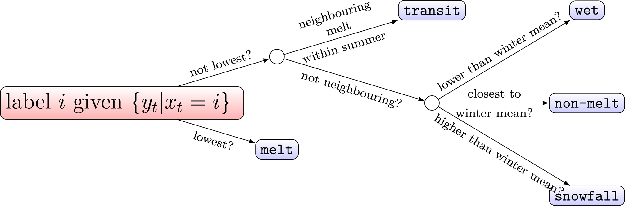
The state-space models recognise five states in total. We name the five states as (1) melt, which refers to the summer melt event, (2) transit, i.e. the intermediate state between two other states, (3) wet (rain-refreezing), which relates to large rainfall events as the surface may start off wet after a rainfall event but it quickly refreezes, (4) nonmelt, which refers to the condition that the surface is not melt and (5) snow cover (large snowfall), which relates to high snowfall or deep snow, as the snow density changes after particularly large snowfall event.
The five states describe temporal variation in the melting process, and the process differs across space as the surface type varies. Here, we consider three surface types ‘snow’ – snow-covered pixels in all seasons in all years, ‘lake’ – open water bodies that appear each spring/summer and ‘ice’ – which may be snow-covered in winter but is bare ice in summer. We also consider ‘dark ice’, which refers to the area of ice with embedded dust and debris making it appear dark.
We evenly sampled pixels across the three surface type to test our method. Based on our analysis of the training sites, the snow pixels are those with mean SAR values higher than 0.8 during nonmelt states. In most of the cases, the nonmelt state has the highest SAR values compared to the other states at the same pixels. A pixel can be characterised as a dark ice pixel if within the corresponding SAR time series, the nonmelt state has mean SAR values lower than 0.05. Pixels that do not fit the snow or black ice criteria are categorised as ice or lake.
Pixels of each type have a different number of states. The three-state snow pixels are viewed as nonmelt, wet and melt states; the four-state ice or lake pixels have an additional transit or snow cover state; and the five-state pixels have the transit states split into before and after melt states. By implementing the state identification algorithm, we manage to identify two of the four surface types sampled, namely, snow and dark ice, while automatically recognising melting patterns at any location regardless of the surface type.
4. Results and discussion
We have used the nine sites to train our state-space model and create the decision framework in Fig. 5. We now apply this decision framework to the study area, at pixels sampled at 6 km spacing. At these pixels, we use the modelling approach to capture the state-switching in the SAR time series values and apply the decision rules to label the pixel surface states. Without any prior information of the selected locations, the algorithm can be used to recognise the surface type, and also changes in the time series are sampled at each location. Results are then verified, post decision, by visual inspection of Landsat optical images and by comparison with MAR output.
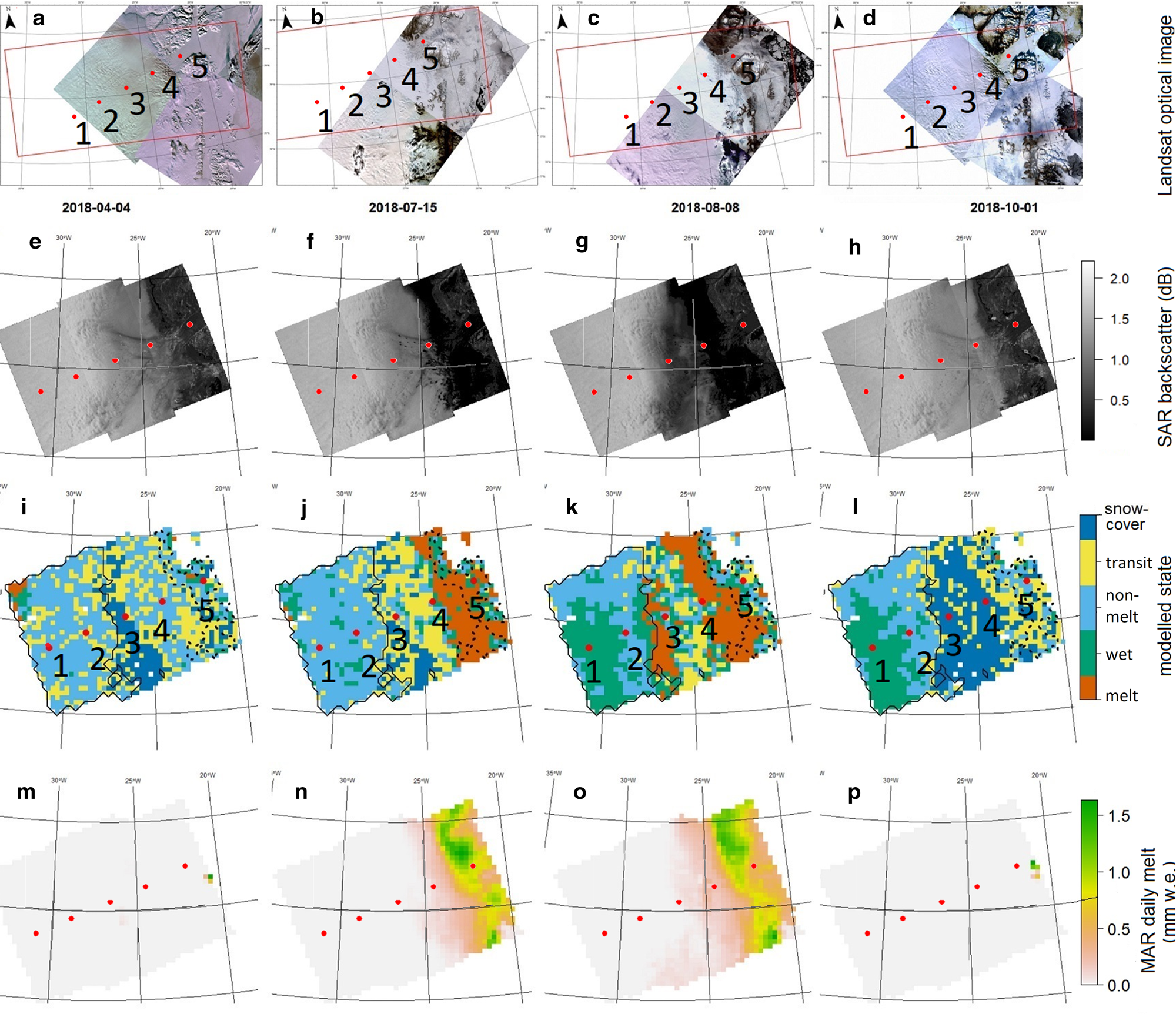
This algorithm performs well in identifying ‘snow’ and ‘dark ice’ regions in this sector of Greenland (Fig. 6). From (i) to (l), the contoured regions with solid line denotes snow and the regions with dashed line outline the dark ice. Indeed, from inspection of optical satellite imagery, it seems that ‘snow’ pixels are associated with the dry snow zone, suggesting that our algorithm is able to identify specific melt facies on the ice sheet. Our algorithm also performs well in picking up temporal variability in surface characteristics. In the dry snow zone, we see a shift from snow cover (high snowfall or deep snow) to wet (rain-refreezing) conditions in the summer of 2018; this corresponds to a widespread rainfall event in this region of Greenland (Fig. 8). In the ‘ice’ or ‘lake’ region of the study area, we see the surface evolve through time from mainly nonmelt and snow cover conditions in April, to transit and melt in July, more extensive melting in August, and then snow cover again in October (Fig. 6). This is the type of behaviour we would expect to see for this part of the ice sheet and indeed correlates well with the pattern of melt spreading up the ice sheet from the margin, as simulated by MAR.
(a)–(p) show the following plots across the four dates throughout 2018: 04/04/2018, 15/07/2018, 08/08/2018 and 01/10/2018.Top row (a)–(d) shows the Landsat tiles collected 3 days within the selected dates. The red polygon in (a)–(d) indicates the study area covered by the SAR images. Row 2 (e)–(h) contains SAR images; row 3 (i)–(l) provides maps of the classified state with snow/black ice contours. The five classified states are coloured in dark blue (snow cover), yellow (transit), blue (nonmelt), green (wet) and orange (melt). Row 4 (m)–(p) shows the daily melt from MAR.
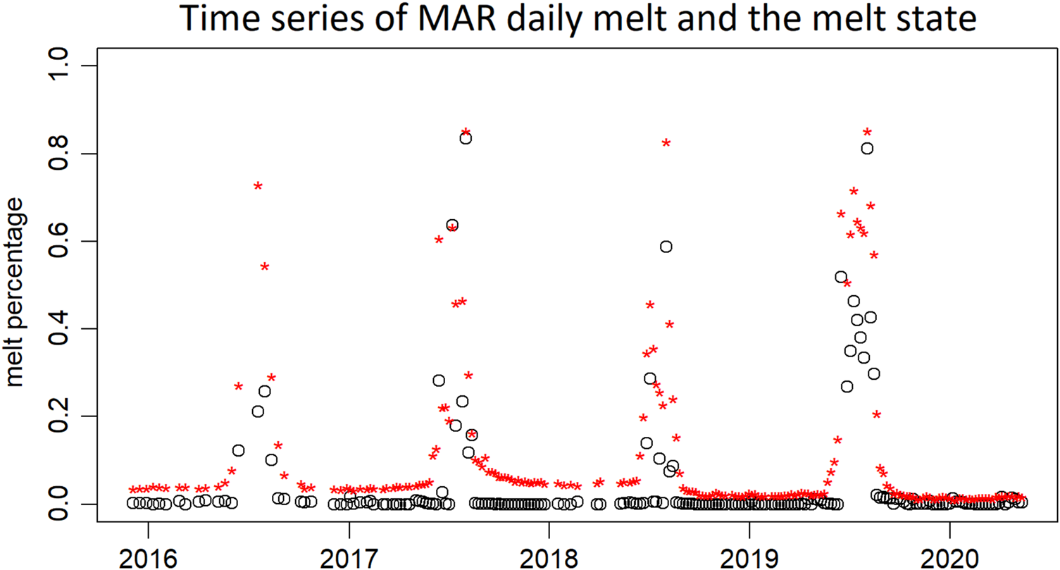
In addition to comparison at the four selected scenes, we calculate the area of the melt state as a percentage of the total study area as a time series to represent temporal variation throughout the whole study period. Figure 7 shows the temporal variability in the surface characteristics. We cross-compare this with the MAR daily melt time series and the figure shows excellent agreement between the two datasets, in terms of both variability and magnitude (with correlation coefficient r = 0.86).
The MAR daily melt (black dots) data, which are threshold above 1 mm d−1 for removing noise, are calculated as the percentage of total study area. The melt state (red stars) is the melt state spatial proportion at each time point.
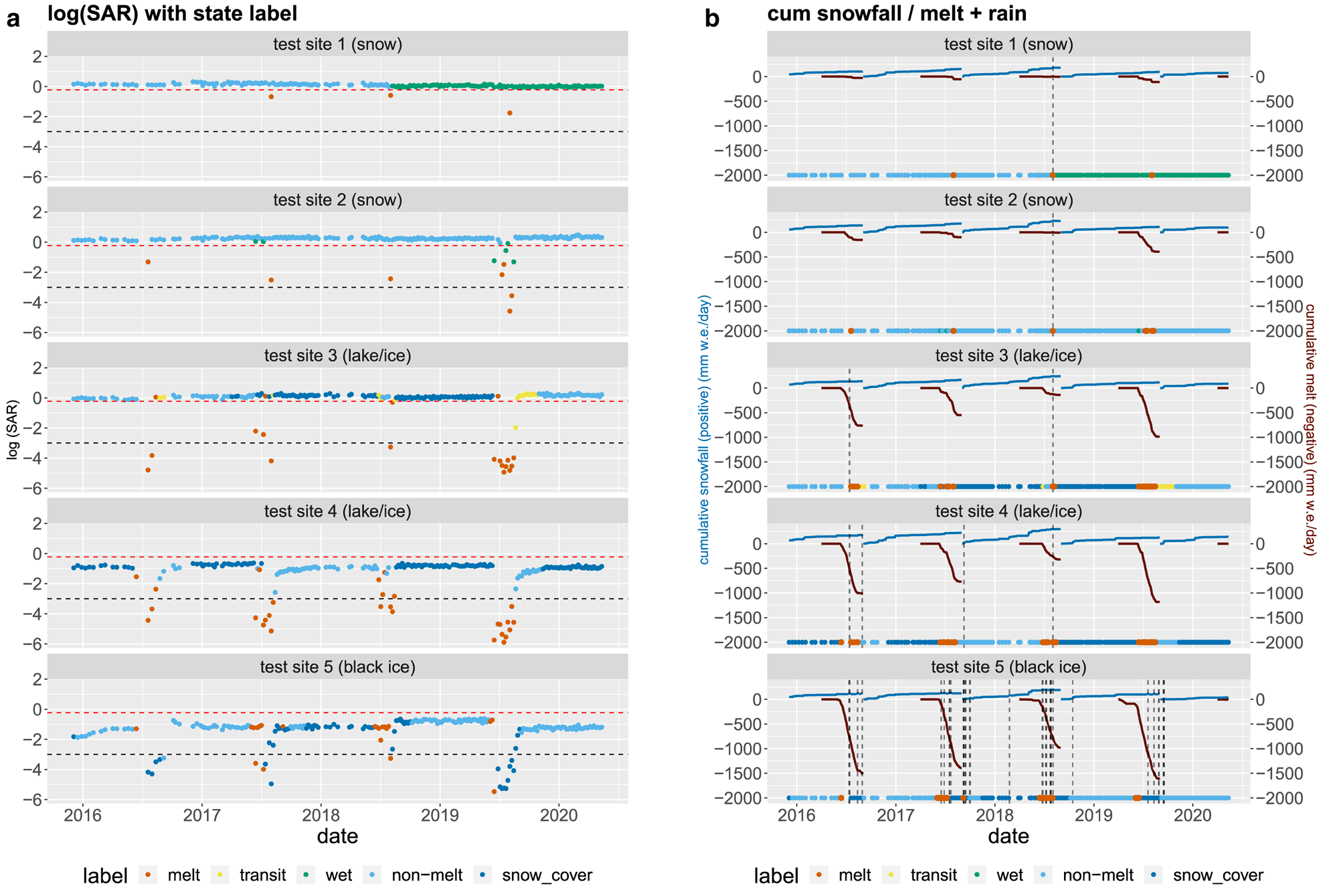
We select five specific testing sites picked at equal spacing from a transect running down the centre of the study area from inland to the coast, to evaluate our method in terms of its ability to correctly classify the evolution of the ice sheet surface over multiple years (Fig. 8). The locations of the five test sites are marked in Figs. 6(i)–(l) as five red dots. The number 1–5 goes from the lower left to the upper right. Test locations 1 and 2 are identified by our algorithm as being snow sites (Fig. 6). From visual inspection of optical satellite imagery (Figs. 6(a)–(d)), it seems reasonable that this is the case, since these sites are located far inland and above the permanent snow line. Test locations 3 and 4 are identified by our algorithm as being either ice or lake sites – it is not yet possible to differentiate between the two using our method. From the optical satellite imagery, this seems reasonable, both sites look like they are below the permanent snow line. Test location 5 is identified as a dark ice site, and indeed from the optical satellite imagery, we can see that this site is located on the debris-covered trunk of the 79 N° glacier.
At test location 1, our algorithm identifies a transition from snow cover (high snowfall or deep snow) to wet (rain-refreezing) in 2018 which, as previously discussed, corresponds well to a widespread rainfall event. Our method identifies melt in the summers of 2017, 2018 and 2019 but misses melt simulated by MAR in 2016. This is likely either due to the time interval of 6-day in the SAR backscatter (the surface may melt between two observations) or because melting in 2016 was insufficient to affect the dielectric properties of the ice sheet surface. The melt period is identified each year (2016–2020) at test location 2, though on some days at the start and the end of the melt season, our algorithm identifies wet (rain-refreezing) conditions which from the MAR data seem more likely to be transit states – as the snowpack starts to melt and as the melted snow surface refreezes. Transit states are identified at test site 3, and melt periods are identified in each year except for the summer of 2018. Here, our method suggests that the surface does not progress beyond a transit state – i.e. it does not fully melt. From MAR, we can see that melting in this year was unusually low at this site, which suggests that an appreciable amount of melting has to occur, before it is identified by our model as a distinct state. At test sites 3 and 4, snow cover states are modelled in winter – from the MAR data, it seems that these are associated with winters where snowfall is high. The performance of our classification algorithm at test site 5 is less convincing; however, this is likely because changes to backscatter at the dark ice site are more subtle and thus harder to differentiate as separate states. Summarising the comparison between results from the five test sites and results from MAR, Fig. 8 shows that our melt states and snow cover states correspond to MAR cumulative melt and cumulative snowfall increases respectively, and the wet (rain-refreezing) states coincide with to MAR rainfall events.
Comparison of SAR state and MAR model output at the five testing sites. (a) Time series of log-SAR backscatter at each of the testing sites with classified state labels; Horizontal lines: red – log (0.8); black – log (0.05). (b) MAR model outputs: proxies for cumulative snowfall (positive) and cumulative melt (negative), rainfall (threshold above 1 mm w.e. d−1) – dashed vertical lines.
5. Conclusion
In this study, we have proposed a method of modelling SAR backscatter time series to understand the melt/state-switching process on the ice sheet surface. After scrutinising the estimated states with optimal images, which inform on the surface type, and the MAR model that provided variables to explain the state-switching process, we established the procedure of identified the melting states while recognising the surface type. The identification of surface types, i.e. snow and dark ice, explains the varying patterns observed at different regions and helps with understanding and recognising the state-switching process throughout the seasons. We show, as a proof of concept, that our algorithm can successfully identify melt facies and dark ice, though at present it is less skilled at differentiating between ice and lake pixels. We show that our algorithm can successfully classify the temporal evolution of the ice surface, and in particular that it can identify seasonal surface melting across a wide area. Finally, we show that our method can recognise changes in the surface ice sheet condition resulting from weather events, such as rainfall or snowfall.
The classification of melt/nonmelt and other additional states were well supported by multiple variables from the MAR models. The classification of the surface type was compared with a limited number of optical images by visual inspection. So far, we conclude our method performs well in recognising the melting process, and the qualitative comparison with optical images shows our method has the potential of recognising the surface type. To achieve accurate classification of the surface type, i.e. snow, ice and lakes, more validation data are needed. The ground truth data for ice sheet surface type are not directly available but there have been recent advances of using optical images to recognise the ice sheet surface, which might be of use to future studies (Vandecrux et.al. 2022). Obtaining the ground truth data is essential for quantifying model uncertainty
Further work is needed to refine the model to develop the method such that it can distinguish between lake and ice pixels. At present, the classification is somewhat noisy, and the temporal evolution of surface characteristics in the dark ice region in particular seems to be poorly captured. Averaging neighbouring pixels in the data preprocessing step may effectively smooth out some of the noise and help achieve better classification results. We also consider incorporating spatial correlation into the state-space model such that neighbouring pixels can share information and introducing temporal and spatial covariates in the model. To further extend our analysis, a hierarchical model structure with a primary level associating with surface type and a secondary level for state-switching process is worth considering. In addition, a semi-Markov model, which estimates a state at every given time instead of just at the state-switching time, may help with improving the results. We would also consider relaxing the state-space model, allowing the number of states to change across sites, for a better representation at some sites where fewer changes occur. This can be achieved by allowing some transition probabilities to be 0 in the state-space model. As a proof of concept, however, and compared to conventional ice sheet melt classification approaches, we show that our method has the potential to yield deeper understanding about the melting process through identifying a wide range of ice sheet surface states. Our method is particularly valuable since Sentinel-1 SAR data are of a high spatial resolution (higher resolution than climate models). Thus in developing a method to identify the state of the surface from these data, we improve our capability to understand the spatial distribution of ice sheet melting and how this varies through time.
Data
Raw data were generated at ESA https://sentinel.esa.int/web/sentinel/sentinel-data-access. Derived data supporting the findings of this study are available from the corresponding author Q.S on request.
Acknowledgements
The authors grateful acknowledge Mal McMillan for helpful comments on an early draft. We are grateful for the technical assistance of Prateek Gantayat and Thomas Barnes. This research was supported by grants from the Engineering and Physical Sciences Research Council (EP/R01860X/1, EP/S00159X/1 and EP/V022636/1) and Natural Environment Research Council (NE/T012307/1).
Author Contributions
Conceptualisation: Qingying Shu; Rebecca Killick; Amber Leeson; Christopher Nemeth; David Leslie. Methodology: Qingying Shu; Rebecca Killick; Amber Leeson; Christopher Nemeth. Data curation: Qingying Shu; Amber Leeson; Xavier Fettweis; Anna Hogg.
Data visualisation: Qingying Shu; Amber Leeson; Xavier Fettweis. Writing original draft: Qingying Shu; Rebecca Killick; Amber Leeson; Christopher Nemeth. All authors approved the final submitted draft.
Appendix A.
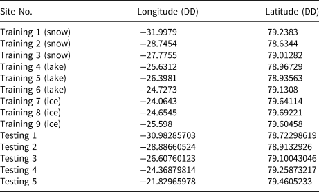
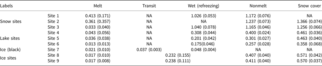
The time series of SAR backscatter we analyzed are taken at nine pre-labelled training sites and five testing sites. The longitude and latitude of the training and testing sites are listed in Table 1. State-space model parameters, including the state mean and the state variance, are estimated across sites. Table 2 lists the model parameters from the nine training sites.
Longitude and latitude of the nine training sites and the five testing sites in decimal degrees (DD)
State-space model parameters, including the state mean $\hat {\mu }$ and the state variance $\hat {\sigma }^2$
 . $\hat {\mu } ( \hat {\sigma }^2)$
 were estimated for the five states across the 9 training sites
Appendix B.
The additional meteorological variable obtained from the MAR climate model include albedo and 0–10 cm surface snow density (kg m−3) in Fig. 9, for comparing with the melt and nonmelt states detected from the SAR data at the nine training sites. The orange melt states occur at albedo trough and density peak. Snow height evolution, obtained from the MAR accumulated snowheight change variable, is shown in Fig. 10 together with the SAR snow states, indicated by the grey vertical lines. The variable is plotted together with the cumulative snowfall in light blue. This suggests that the snow states can be detected after a sufficient amount of snowfall, regardless of snow height change.
Comparison of melt/nonmelt state with MAR albedo/0–10 cm surface density (kg m−3).
Comparison of snow cover state and snow height evolution/cumulative snowfall.
Appendix C.
C.1. State-space model
Assuming the states, x t, are a Markov chain taking values in a finite state space {1, ⋅ ⋅ ⋅ , K}, where K = 5 in our context. The hidden state process {x t}, t ∈ T is categorical and can be written as a multinomial vector. Let $x_t^k$ be a binary indicator for whether x t is in state k ∈ {1, ⋅ ⋅ ⋅ , K}. The tth hidden state is k if $x_t^k = 1$
 . The transition probability P (x t|x t−1) is the probability that the model is in state x t at time t given that the model was in state x t−1 at time t − 1. This forms a transition matrix A = {a jk}, j, k ∈ {1, ⋅ ⋅ ⋅ , K}, for describing the probability of $x_t^k = 1$
 , i.e. the tth state is k, conditioned on $x_{t-1}^j = 1$
 , i.e. the t − 1th state is j. The emission probabilities P(y t|x t) specify the probability distribution for the observation y t, given the model is in state x t at time t.
C.1.1. Parameter estimation
We fit the hidden Markov state-space model to the time series of the pixel values using the R package depmixS4. depmixS4 provides a framework for specifying and fitting hidden Markov models using the expectation–maximisation (EM) algorithm for optimisation. Expectation–maximisation is an iterative procedure that maximises the model's likelihood function. Let θ (s) be the set of parameter estimates from the s-th iteration of the EM algorithm. The computation in the E-step uses information from the observed data {y t} and the parameter estimates θ (s) from the preceding M-step. The required expected sufficient statistics for the EM algorithm are $E[ x_1^k]$ and $E[ x_t^j x_{t + 1}^k]$
 .
.
The basic idea behind the EM algorithm is that directly maximising the log-likelihood $\log p( {{\cal Y}}\vert \theta )$ is intractable as there is no explicit form for $p( {{\cal Y}}\vert \theta )$
 . However, the joint log-likelihood $\log p( {{\cal Y}},\; {{\cal X}}\vert \theta )$
 is available and can be maximised iteratively as follows:
Iterate:
E-step: Find $Q( \theta \vert \theta ^{( l) }) = E[ \log p( {{\cal Y}},\; {{\cal X}}) \vert \theta ^{( l) }]$
M-step: Find $\theta ^{( l + 1) } = \hbox {argmax}_\theta Q( \theta \vert \theta ^{( l) })$
C.1.2. Model selection and optimal number of states
At a random location, the time series of pixel SAR values could range from two to five states, representing a switch in the ice sheet surface properties. In fitting the state-space model to each time series, the number of states can take the values of 2, 3, 4 or 5. Four models each with a different number of states are fitted to time series at each location.
We do not know the number of states in advance, and so we fit the state space model with different n, where n represents the number of hidden states, and use the Bayesian information criterion (BIC) (Van Erven and others, Reference Van Erven, Grünwald and de Rooij2012), a criterion for model selection among a finite set of models and the model with the lowest BIC is preferred, to select the best fit and determine n. BIC is defined as follows:
where L is the likelihood, K is the number of model parameters and N is the number of data points used to train the model.
Based on the lowest BIC score, the best-fit model for SAR time series at each site is selected. The optimal number of states is subsequently recognised as indicated by the best fitting model.


 Open access