





1 Introduction
The increasing use of computer-based assessments and digital technologies has produced extensive behavioral data for educational and psychological research. Among these, eye-tracking has become a valuable method for examining cognitive and behavioral processes. Prior studies have used eye-tracking data to uncover cognitive mechanisms during testing (Kaczorowska et al., Reference Kaczorowska, Plechawska-Wójcik and Tokovarov2021; Zhu & Feng, Reference Zhu and Feng2015), describe test-taking behaviors (Man & Harring, Reference Man and Harring2023), and gather validity evidence for item and test design (Yaneva et al., Reference Yaneva, Clauser, Morales and Paniagua2021, Reference Yaneva, Clauser, Morales and Paniagua2022). In particular, applications to mental rotation tasks have provided important insights into spatial reasoning, problem-solving strategies, and gender-related differences in cognitive processing (e.g., Nazareth et al., Reference Nazareth, Killick, Dick and Pruden2019; Xue et al., Reference Xue, Li, Quan, Lu, Yue and Zhang2017).
Our motivation data set stems from an experiment that used a spatial rotation learning program (Wang et al., Reference Wang, Wu, Chen, Fang, Xiao and Li2026, Reference Wang, Hu, Wang, Wu, Shen and Carr2020) to assess participants’ mental rotation skills. The program includes two test blocks and two learning blocks, with learning blocks placed between the test blocks. Each block has 10 multiple-choice questions, with the learning blocks featuring additional interactive elements. Eye-tracking equipment captured participants’ eye-movement data during the experiment, which generated a rich array of data that capture both static and dynamic aspects of visual behavior. Typically, eye-tracking systems record raw gaze coordinates over time, which can then be processed into summary eye-movement metrics, such as fixation duration and count, saccade length and velocity, number of glances, and visit frequency or duration within predefined areas of interest (AOIs).
Beyond these aggregated indicators, eye-tracking devices also provide temporal sequences of gaze events—including the order, duration, and transitions between fixations and saccades—offering fine-grained representations of an individual’s eye-movement trajectory during task performance. An example is shown in Figure 1 for one participant’s fixation sequence in one test question. The action
$A_t$
 represents the fixation location on an area of interest at time point t, and the duration of each fixation and the elapsed time between two consecutive fixations are also available. Such sequential data enable researchers to explore dynamic patterns of visual attention and information processing that cannot be captured by summary statistics alone (e.g., Liu & Cui, Reference Liu and Cui2025).
The example of the fixation sequence for one participant on one question.

Compared with aggregated indicators, unstructured eye-tracking sequence data retain richer, fine-grained information about individual differences. Although our focus is on eye-tracking sequences, their analytic value can be understood within the broader process-data framework, where prior studies have demonstrated how process data can be used to model latent traits, improve proficiency scoring, identify behavioral prototypes, and predict performance outcomes (Chen, Reference Chen2020; Fang & Ying, Reference Fang and Ying2020; He et al., Reference He, von Davier and Han2019, Reference He, Shi and Tighe2023; LaMar, Reference LaMar2018; Liu et al., Reference Liu, Liu and Li2018; Tang, Reference Tang2023; Ulitzsch, Molter, et al., Reference Ulitzsch, Molter and Pohl2022; Zhang, Wang, et al., Reference Zhang, Wang, Qi, Liu and Ying2022). These findings suggest that unstructured eye-movement sequences likewise offer rich diagnostic potential for understanding how individuals engage with tasks and solve problems.
The goal of this case study is to analyze both structured data (binary response scores) and unstructured data (eye-movement sequences) from the testing and learning blocks to provide construct validity evidence about participants’ testing and learning behaviors. Specifically, we address six research questions (RQ): For testing behaviors, we ask (RQ1) what participants’ testing behaviors are in Test Blocks 1 and 2, (RQ2) how these behaviors change between the two blocks and relate to different question types, and (RQ3) how testing behaviors are associated with overall test performance. For learning behaviors, we examine (RQ4) what participants’ learning behaviors are in Learning Blocks 1 and 2, (RQ5) how these behaviors vary across question types, and (RQ6) how learning behaviors are associated with testing behaviors to better understand the linkage between learning and assessment processes.
The research questions on testing behaviors (RQ1–RQ3) aim to examine participants’ problem-solving processes and explore how variations in response patterns relate to question types and performance outcomes. These analyses are expected to yield construct validity evidence for the test items and provide deeper insights into participants’ testing performance. Likewise, the research questions on learning behaviors (RQ4–RQ6) focus on how participants engage with learning materials, how these behaviors vary by question type, and how learning behaviors influence subsequent testing behaviors. Findings from these analyses will contribute validity evidence for the learning design and inform potential refinements to the integration of learning and assessment components.
To answer these questions, we must address the challenges inherent in analyzing dynamic, high-dimensional, and multimodal data. The dynamic nature arises from the platform’s design, which records data across multiple time points, while the high-dimensional and multimodal aspects stem primarily from the eye-tracking sequences that capture fixation durations and inter-action intervals across four blocks. To tackle these challenges, we propose a data analytic framework (DAK) comprising two integrated components that address two key issues: (1) analyzing unstructured, high-dimensional sequence data and (2) integrating and interpreting evidence across multiple analytic results.
The first component of the DAK proposes a new time-aware long short-term memory (T-LSTM) Autoencoder framework for feature extraction. This framework builds on existing LSTM research (Min et al., Reference Min, Frankosky, Mott, Rowe, Smith, Wiebe, Boyer and Lester2019; Yin et al., Reference Yin, Alqahtani, Feng, Chakraborty and McGuire2021) by incorporating the duration of actions and the elapsed time between consecutive actions, along with the original eye-movement sequence, providing a more comprehensive analysis of eye-tracking data. We demonstrated the effectiveness of this new feature extraction method and provided guidance on how to select the best Autoencoder model based on different hyperparameters. The second component of our DAKs provides systematic guidelines for interpreting the patterns captured in extracted features through an integrated suite of data-analytic tools. When interpreted appropriately, process data (e.g., log files, eye-tracking sequences, and response times) can provide construct-relevant evidence by revealing whether the strategies and behaviors observed during problem solving align with those anticipated in the evidence model (He et al., Reference He, Borgonovi and Paccagnella2021; Wang et al., Reference Wang, Mousavi, Lu and Gao2023). However, a major challenge in applying feature extraction methods to educational assessment tasks lies in the limited interpretability of the extracted features, which often hinders their direct use in addressing substantive research questions. Specifically, we employed a series of statistical analyses, including (a) clustering analyses of extracted features to identify distinct patterns of test-taking and learning behaviors, (b) categorical data analysis techniques to summarize and compare changes in these patterns, thereby providing evidence for the quality of assessment design and the effectiveness of learning interventions, and (c) generalized mixed-effects models to examine the relationships between test-taking behaviors and test performance.
The remainder of this article begins with a description of the motivating dataset and an overview of the proposed DAK. We then detail the two components of the DAK and demonstrate their application in addressing the six research questions using the motivating data. Finally, we conclude with a discussion of key findings, limitations, and directions for future research.
2 Motivation data and overview of the proposed DAK
The structured and unstructured data are from a sample of 70 participants with their interaction of a spatial rotation learning platform, which are summarized in Table 1.Footnote 1 For each participant, the structured data include binary response scores for all items in both the test and learning blocks, while the unstructured data consist of eye-movement sequences recorded during task performance. Among various eye-tracking metrics, we focus on fixation sequences, as fixation patterns are well-established indicators of how individuals allocate attention and process information. Longer or more frequent fixations often reflect greater cognitive effort or uncertainty in decision-making (e.g., Rayner, Reference Rayner1998, Reference Rayner2009). In this study, our primary goal is to enhance the interpretability of test-takers’ testing and learning behaviors using features derived from eye-tracking sequences, rather than focusing on predictive tasks such as score prediction. An earlier work has conducted a multidimensional exploratory analysis on using 100 eye-tracking summary variables and participants’ response score and response time in one test block from this experiment and discovered that the latent structures extracted from fixation-related variables can offer meaningful insights into individuals’ test-taking processes (Wang et al., Reference Wang, Wu, Chen, Fang, Xiao and Li2026). Based on these considerations, we include only fixation sequence data in the following analyses.
Structured and unstructured data from each participant

Table 1 Long description
The table consists of four columns: Block, Number of Questions, Structured data, and Unstructured data.
* The first row under the headers lists blocks T B 1 and T B 2. It specifies 10 questions for each block. The structured data is a Binary score, and the unstructured data is a Fixation sequence.
* The second row lists blocks L B 1 and L B 2. The Number of Questions and Structured data columns are empty for these blocks. The Unstructured data column contains the details: action location, duration, and elapsed time.
A note below the table clarifies that T B represents the test block and L B denotes the learning block.
Note: TB represents the test block, and LB denotes the learning block.
2.1 The complexity of unstructured eye fixation sequence data
An eye fixation sequence with temporal and sequential dependencies is shown in Figure 1. For this experiment, a participant’s fixation sequence on a question contains six unique locations as described by Figure 2. Look_1 denotes location on the first object (initial position) in the example rotation; Look_2 represents the second object (ending position) in the example rotation; and Look denotes other parts of the Look area. Question denotes the central part (circled in red), which represents the new object to be mentally rotated; option_correct denotes the location of the correct answer in the multiple-choice options; and option_wrong is the location on any of incorrect options.
Example of a fixation sequence from one participant to one question.

Figure 2 Long description
The interface is divided into three horizontal sections.
At the top, two 3D block shapes are shown. The left shape is labeled Look underscore 1 and the right shape is labeled Look underscore 2. Between them is the text After rotation, become. A large red and yellow heatmap intensity, labeled Look, is centered over this text, with smaller intensities over the two shapes.
The middle section is enclosed in a thick red box labeled question. It contains the text After rotation as above, followed by a 3D semi-cylindrical shape, and then the text will become. Light green heatmap spots are scattered across this area.
The bottom section displays five multiple-choice options labeled A through E, each showing a different orientation of the semi-cylindrical shape. Option B is enclosed in a red box.
Arrows at the very bottom categorize the selections. A red arrow points from the red box around Option B to the label Option underscore correct. Blue arrows point from the labels for A, C, and D to the label Option underscore wrong.
The learning platform includes seven types of questions across two test blocks and two learning blocks, measuring rotations in one or two directions along the x or y axis for
$90$
 or
$180$
or
$180$
 degrees (
$x90$
degrees (
$x90$
 ,
$x180$
,
$x180$
 ,
$y90$
,
$y90$
 ,
$y180$
,
$y180$
 ,
$x90y90$
,
$x90y90$
 ,
$x90y180$
,
$x90y180$
 ,
$x180y90$
,
$x180y90$
 ). Details of the design can be found in Table 2 of Wang, Zhang, et al. (Reference Wang, Zhang and Shen2020). The questions in four blocks follow the same format (Figure 2), with the key difference being that participants were not informed of their response accuracy in the test blocks, while in the learning blocks, they were given feedback on correctness and had the opportunity for additional learning interventions.
2.1.1 High dimensionality
The first challenge to address fixation sequences is their high dimensionality and nonstandard format. Consider the fixation sequence data from 70 participants answering 10 questions in test block 1. Treating each participant’s sequence for one question as a single observation gives 700 observations, each with a varying number of variables. As shown in Figure 3, the length of eye-tracking sequences varies widely. For instance, the average sequence length is 430, but some exceed 1,000, reaching up to 2,000, far surpassing the sample size. This high-dimensional sequence data presents challenges for traditional statistical methods.
The distribution of fixation sequence lengths for test block 1.

Figure 3 Long description
The histogram plots Frequency on the vertical Y-axis, ranging from 0 to 70 in increments of 10, against fixation sequence length on the horizontal X-axis, ranging from 0 to 2000 in increments of 500.
* The distribution is positively skewed, with the highest concentration of data points occurring at the lower end of the scale.
* A primary peak reaches a frequency of 70 at a sequence length of approximately 250.
* A secondary, smaller peak occurs around the 500 mark with a frequency of approximately 40.
* Beyond 500, the frequency steadily declines, showing a long tail that extends toward 2000.
* Between 1000 and 2000, frequencies remain low, mostly under 10, with several small gaps where no data is recorded.
Distribution of fixation duration for each action (test block 1).

Figure 4 Long description
A violin plot displays the distribution of fixation durations across six categories on the X-axis. The Y-axis is labeled Duration Time in m s, ranging from 0 to 600 with increments of 200. Each category features a colored violin shape representing density, with an internal white box plot showing the median, interquartile range, and whiskers extending to outliers.
Moving from left to right along the X-axis:
* look: Light green violin. The distribution is concentrated below 200 m s but has a very long thin tail reaching up to 700 m s. The median is approximately 100 m s.
* look_1: Pale yellow violin. Similar distribution to look, with a tail reaching nearly 600 m s and a median around 100 m s.
* look_2: Light purple violin. Distribution concentrated at the bottom with a tail reaching 500 m s. Median is roughly 100 m s.
* option_correct: Light red violin. A wider base at the bottom with a shorter tail reaching approximately 350 m s. The median is lower, around 60 m s.
* option_wrong: Light blue violin. Similar shape to option_correct, with a tail reaching nearly 400 m s and a median around 70 m s.
* question: Light orange violin. A wider distribution in the lower range with a tail reaching 500 m s. The median is approximately 80 m s.
A legend on the right side maps the colors to the action names: look, look_1, look_2, option_correct, option_wrong, and question.
2.1.2 Motivation of considering fixation duration
To preliminarily examine whether integrating fixation duration with fixation location provides a more informative basis for distinguishing testing and learning patterns, we analyzed the distribution of fixation durations in Test Block 1 (Figure 4). The results show that fixation duration distributions vary notably across locations. For instance, locations, such as “look” and “question,” display wider ranges and longer tails, indicating greater variability, whereas “option_correct” and “option_wrong” exhibit more compact distributions. These findings suggest that fixation duration captures meaningful differences across action types and should be examined in conjunction with fixation location sequences when analyzing testing and learning behaviors.
2.1.3 Motivation of considering elapsed time
To examine how elapsed time between consecutive fixations influences transitions, we divided all fixation pairs into five subsets based on quartiles of the elapsed time distribution: Q1 (elapsed times below the 1st quartile), Q2 (between the 1st quartile and median), Q3 (median to 3rd quartile), Q4 (above the 3rd quartile but below 3000 ms), and a final subset for extremely long elapsed times (>3,000 ms). For each subset, we constructed a
$6 \times 6$
 transition matrix to represent the probabilities of transitioning between locations. Each element
$(i,j)$
transition matrix to represent the probabilities of transitioning between locations. Each element
$(i,j)$
 in the matrix represents the probability of transitioning from action i to action j, estimated using the proportion of observed transitions in this cell relative to all transitions. Figure 5 displays these matrices from test block 1. In Q1, participants primarily remain within the same location, indicating that shorter elapsed times strengthen the influence of the current fixation. As elapsed time increases (up to Q4), location transitions become more evenly distributed, reflecting a reduced fixation influence. This trend is most noticeable in the final matrix, where transition probabilities approximate a uniform distribution for very long elapsed times (>3,000 ms). These findings highlight the importance of considering elapsed time when analyzing fixation transitions.
Five transition patterns of consecutive fixations for test block 1 sequences.

Figure 5 Long description
A multi-panel figure containing five heatmaps arranged in two rows. The top row contains three heatmaps labeled Q 1, Q 2, and Q 3. The bottom row contains two heatmaps labeled Q 4 and greater than 3000. A vertical color scale on the far right indicates probability from 0.00 in white to 1.00 in dark red.
Each heatmap shares the same axes. The vertical y-axis is labeled From and the horizontal x-axis is labeled To. Both axes contain six categories in the following order from bottom to top and left to right: look, look underscore 1, look underscore 2, option underscore correct, option underscore wrong, and question.
* Transition Heatmap Q 1: Shows high concentration along the diagonal and top-right corner. Key values include look underscore 1 to look underscore 1 at 0.94, look underscore 2 to look underscore 2 at 0.93, and question to question at 0.93.
* Transition Heatmap Q 2: Shows a shift toward the center and right. High probabilities include look underscore 1 to look underscore 1 at 0.58 and option underscore wrong to option underscore wrong at 0.66.
* Transition Heatmap Q 3: Similar to Q 2, with look underscore 1 to look underscore 1 at 0.57 and option underscore wrong to option underscore wrong at 0.63.
* Transition Heatmap Q 4: Shows more distributed probabilities. Highest values are look underscore 2 to look underscore 1 at 0.56 and question to question at 0.57.
* Transition Heatmap greater than 3000: Displays the most dispersed probability distribution. The highest single value is option underscore wrong to option underscore wrong at 0.49, followed by look underscore 1 to look underscore 1 at 0.44.
2.2 Overview of the two-component DAK
We propose a comprehensive two-component DAK for complex, high-dimensional structured and unstructured data, as shown in Figure 6.
The proposed data analytic framework.

Figure 6 Long description
The flowchart consists of four main blocks connected by right-pointing arrows.
1. Input for D A K Component 1: Unstructured Data. This first block lists three bullet points: Fixation location sequence, Fixation duration sequence, and Elapsed time duration sequence.
2. Analytic Tools. The second block lists: Feature extraction: T-L S T M Autoencoder, Model Selection and Evaluation, and Output: latent features.
3. Input for D A K Component 2. The third block lists: Latent features from D A K component 1 and Structured data: item score.
4. Analytic Tools. The final block lists three main tasks:
• Clustering Latent features (Summarize Pattern).
• Interpretations: summary statistics, pie chart and transition matrix.
• Explore relationships: Contingency Table Analysis and G L M M.
The first component addresses the challenges of analyzing unstructured data with temporal and sequential dependencies. Specifically, it examines two key questions: (1) how to effectively extract features from high-dimensional fixation sequence data by incorporating both fixation durations and elapsed times between consecutive fixations and (2) how to identify the optimal feature extraction model using an appropriate evaluation mechanism. The second component focuses on integrating and interpreting evidence from multiple analytic results to answer educationally meaningful research questions in the context of the spatial rotation experiment. Sections 3 and 4 provide details of these two components.
3 DAK component 1
3.1 Rationale of the DAK component 1
Existing approaches for analyzing unstructured, unsegmented sequence data have been studied in the psychometrics (He & Cui, Reference He and Cui2025), process mining (Bogarín et al., Reference Bogarín, Cerezo and Romero2018), and natural language processing literature. They can generally be categorized into several types. One category relies on summary variables or similarity measures derived from raw sequences (Hahn & Klein, Reference Hahn and Klein2025; Ivanová et al., Reference Ivanová, Laco and Benesova2022; Liu & Cui, Reference Liu and Cui2025; Schnipke & Scrams, Reference Schnipke and Scrams1997; Ulitzsch et al., Reference Ulitzsch, He, Ulitzsch, Molter, Nichterlein, Niedermeier and Pohl2021). The features or pairwise sequence similarity measures are often used to identify clusters of sequential patterns (Križanić, Reference Križanić2020; Song et al., Reference Song, Günther and Van der Aalst2008; van Dongen & Adriansyah, Reference van Dongen and Adriansyah2009; Yang et al., Reference Yang, Cai and Hu2022) that reflect meaningful individual differences. However, the outcomes of such approaches are typically sensitive to how these summary features or dissimilarity measured are defined.
Another category of approaches focuses on data-driven feature extraction from the raw sequences, preserving temporal and sequential pattern information in a data-driven manner. Without pre-specifying a subset of patterns/characteristics to attend to, these methods could yield more faithful representations of underlying individual differences in behavioral or cognitive processes, but at the same time can be more difficult for interpretation. Accordingly, the first component of our analytic framework is designed to extract data-driven features from unstructured data while retaining their temporal and sequential dependencies.
Although various feature extraction techniques have been applied to process data across educational and behavioral domains (e.g., He et al., Reference He, Borgonovi and Paccagnella2021; Min et al., Reference Min, Frankosky, Mott, Rowe, Smith, Wiebe, Boyer and Lester2019; Pardos et al., Reference Pardos, Baker, San Pedro, Gowda and Gowda2014; Peña-Ayala, Reference Peña-Ayala2014; Tang et al., Reference Tang, Wang, He, Liu and Ying2020; Zhang et al., Reference Zhang, Taub and Chen2022, Reference Zhang, Li and Wang2023), only a few incorporate timestamp sequences alongside process data (Tang et al., Reference Tang, Zhang, Wang, Liu and Ying2021; Ulitzsch et al., Reference Ulitzsch, He, Ulitzsch, Molter, Nichterlein, Niedermeier and Pohl2021). Moreover, even when temporal information is considered, different types of timing information, such as action duration and time intervals between actions, are rarely differentiated.
In the context of eye-tracking fixation sequences, accounting for different types of time-related information, such as fixation durations and the elapsed time between consecutive fixations, is essential (see Figure 1). Two participants may focus on the same locations in the same order, yet their problem-solving strategies can differ substantially based on their temporal patterns. Variations in fixation duration and inter-fixation intervals can reveal meaningful differences in attention allocation, cognitive load, and decision-making strategies.
Autoencoder model structure. (a) Overall architecture incorporating temporal information. (b) Notation and data representation at the sequence level.

Figure 7 Long description
Panel a illustrates the overall architecture. On the far left, a vertical blue box contains a sequence from s sub 1 to s sub N. An arrow labeled Embed s sub i through h sub e points to a yellow Input block. This block consists of Action embedding E sub 1 through E sub N, which is added to Time info columns l sub 1 through l sub N and d sub 1 through d sub N. This combined input enters a green trapezoidal T L S T M Encoder. The encoder compresses data into a central orange rectangular Latent feature. A second green trapezoidal T L S T M Decoder expands the latent feature into a blue output embedding box containing O-hat sub 1 through O-hat sub N. From the output embedding, two paths emerge. A classifier path leads to a blue box with P sub 1 through P sub N, which connects back to the original s sequence via a dashed blue line labeled Cross-entropy loss. A regressor path leads to a yellow box with l-hat and d-hat sequences, connecting back to the input time info via a dashed orange line labeled M S E loss.
Panel b defines the notation for these variables as matrices. s sub i is a column vector from s sub i,1 to s sub i,T sub i. E sub i is a matrix of e values with dimensions T sub i by k. l sub i and d sub i are column vectors of length T sub i. O-hat sub i is a matrix of o-hat values with dimensions T sub i by k. P sub i is a matrix of p values with dimensions T sub i by 6.
3.2 The proposed Autoencoder with T-LSTM
We now introduce an Autoencoder model (Hinton & Salakhutdinov, Reference Hinton and Salakhutdinov2006) to extract hidden features from fixation sequence data. The model incorporates both fixation sequences and their corresponding time and elapsed time data, integrating temporal information into feature extraction. The encoder and decoder use a novel T-LSTM framework, which captures the impact of elapsed time on subsequent actions.
Let
$\mathcal {S}=\{ \mathbf {s}_i\}_1^N$
 denote the fixation sequences, where N is the total number of sequences. The
$i^{th}$
denote the fixation sequences, where N is the total number of sequences. The
$i^{th}$
 sequence,
$\mathbf {s}_i=\left (s_{i,t}, \ldots , s_{i, T_i}\right )^T$
sequence,
$\mathbf {s}_i=\left (s_{i,t}, \ldots , s_{i, T_i}\right )^T$
 , represents the sequence of actions, with
$s_{i,t}$
, represents the sequence of actions, with
$s_{i,t}$
 being the
$t^{th}$
being the
$t^{th}$
 action and
$T_i$
action and
$T_i$
 the total number of actions. Each action corresponds to one of six fixation locations:
$\mathcal {A}=$
the total number of actions. Each action corresponds to one of six fixation locations:
$\mathcal {A}=$
 {Look, Look_1, Look_2, Question, Option_correct, and Option_wrong}. Additionally, the time duration sequence for the
$i^{th}$
{Look, Look_1, Look_2, Question, Option_correct, and Option_wrong}. Additionally, the time duration sequence for the
$i^{th}$
 sequence is denoted as
$\mathbf {d}_i=\left (d_{i, t}, \ldots , d_{i, T_i}\right )^T$
sequence is denoted as
$\mathbf {d}_i=\left (d_{i, t}, \ldots , d_{i, T_i}\right )^T$
 , where
$d_{i,t}$
, where
$d_{i,t}$
 represents the duration of the
$t^{th}$
represents the duration of the
$t^{th}$
 action. The elapsed time sequence is
$\mathbf {l}_i=\left (0, l_{i, 2}, \ldots , l_{i, T_i}\right )^T$
action. The elapsed time sequence is
$\mathbf {l}_i=\left (0, l_{i, 2}, \ldots , l_{i, T_i}\right )^T$
 , where
$l_{i,t}$
, where
$l_{i,t}$
 denotes the time between actions
$s_{i,t-1}$
denotes the time between actions
$s_{i,t-1}$
 and
$s_{i,t}$
and
$s_{i,t}$
 . The Autoencoder model, illustrated in Figure 7, extracts representative features from the eye-tracking sequence
$\mathbf {s}_i$
. The Autoencoder model, illustrated in Figure 7, extracts representative features from the eye-tracking sequence
$\mathbf {s}_i$
 with the help of both time information
$\mathbf {l}_i$
with the help of both time information
$\mathbf {l}_i$
 and
$\mathbf {d}_i$
and
$\mathbf {d}_i$
 . The following sections detail key components of this framework.
3.2.1 Input
The categorical actions in
$\mathbf {s}_i$
 pose a challenge for neural networks due to the absence of inherent numerical relationships. To overcome this, we convert each action into a numerical embedding vector of size k using a learnable embedding layer (Bengio et al., Reference Bengio, Ducharme, Vincent and Jauvin2003; Hancock & Khoshgoftaar, Reference Hancock and Khoshgoftaar2020; Mikolov, Reference Mikolov2013). Mathematically, the embedding layer is parameterized by a learnable matrix
$\mathbf {W}_e \in \mathbb {R}^{6 \times k}$
pose a challenge for neural networks due to the absence of inherent numerical relationships. To overcome this, we convert each action into a numerical embedding vector of size k using a learnable embedding layer (Bengio et al., Reference Bengio, Ducharme, Vincent and Jauvin2003; Hancock & Khoshgoftaar, Reference Hancock and Khoshgoftaar2020; Mikolov, Reference Mikolov2013). Mathematically, the embedding layer is parameterized by a learnable matrix
$\mathbf {W}_e \in \mathbb {R}^{6 \times k}$
 , where
$6$
, where
$6$
 is the number of unique actions and k is the embedding size. For each action
$s \in \mathcal {A}$
is the number of unique actions and k is the embedding size. For each action
$s \in \mathcal {A}$
 , the embedding vector
$\mathbf {e} \in \mathbb {R}^k$
, the embedding vector
$\mathbf {e} \in \mathbb {R}^k$
 :
:

where
$\mathbf {u}_s \in \mathbb {R}^6$
 is a one-hot encoded vector representing the action s, such that the s-th entry is 1 and all others are 0. For each sequence
$\mathbf {s}_i$
is a one-hot encoded vector representing the action s, such that the s-th entry is 1 and all others are 0. For each sequence
$\mathbf {s}_i$
 , the embedding is represented as a matrix
$\mathbf {E}_i=(\mathbf {e}_{i,1}, \dots , \mathbf {e}_{i,T_i})^T$
, the embedding is represented as a matrix
$\mathbf {E}_i=(\mathbf {e}_{i,1}, \dots , \mathbf {e}_{i,T_i})^T$
 with shape
$T_i\times k$
with shape
$T_i\times k$
 , where
$\mathbf {e}_{i,t}=(e_{i,t,1}\dots ,e_{i,t,k})^T$
, where
$\mathbf {e}_{i,t}=(e_{i,t,1}\dots ,e_{i,t,k})^T$
 . By embedding the actions, we map the discrete categories into a continuous vector space, enabling the neural network to better capture semantic relationships between actions.
To capture how time influences these behaviors, we include not only the action sequence
$\mathbf {s}_i$
 but also the corresponding time duration
$\mathbf {d}_i$
but also the corresponding time duration
$\mathbf {d}_i$
 and elapsed time
$\mathbf {l}_i$
and elapsed time
$\mathbf {l}_i$
 , that is, feeding all of them into the Autoencoder model for feature extraction. Mathematically, we concatenate
$\mathbf {E}_i, \mathbf {l}_i$
, that is, feeding all of them into the Autoencoder model for feature extraction. Mathematically, we concatenate
$\mathbf {E}_i, \mathbf {l}_i$
 , and
$\mathbf {d}_i$
, and
$\mathbf {d}_i$
 along the column dimension to form
$\mathbf {X}_i=\left [\mathbf {E}_i, \mathbf {l}_i, \mathbf {d}_i\right ]$
along the column dimension to form
$\mathbf {X}_i=\left [\mathbf {E}_i, \mathbf {l}_i, \mathbf {d}_i\right ]$
 , which serves as the input to the Autoencoder.
3.2.2 Encoder and decoder with T-LSTM framework
The Autoencoder model includes two primary parts: an encoder and a decoder. The encoder compresses the input
$\mathbf {X}_i$
 into a latent representation
$\mathbf {z}_i$
into a latent representation
$\mathbf {z}_i$
 , formulated as

where
$\mathbf {z}_i\in \mathbb {R}^h$
 is intended to capture high-level features of the input sequence i with dimension h. That is,
$\mathbf {z}_i$
is intended to capture high-level features of the input sequence i with dimension h. That is,
$\mathbf {z}_i$
 represents the key feature of the original input
$\mathbf {X}_i$
represents the key feature of the original input
$\mathbf {X}_i$
 and serves as the compressed feature representation used for subsequent analysis. Ideally, if
$\mathbf {z}_i$
and serves as the compressed feature representation used for subsequent analysis. Ideally, if
$\mathbf {z}_i$
 fully captures the information hidden in
$\mathbf {X}_i$
fully captures the information hidden in
$\mathbf {X}_i$
 , then we should be able to reconstruct
$\mathbf {X}_i$
, then we should be able to reconstruct
$\mathbf {X}_i$
 based solely on
$\mathbf {z}_i$
based solely on
$\mathbf {z}_i$
 . Thus, the decoder reconstructs the original
$\mathbf {X}_i$
. Thus, the decoder reconstructs the original
$\mathbf {X}_i$
 from
$\mathbf {z}_i$
from
$\mathbf {z}_i$
 through

confirming that
$\mathbf {z}_i$
 effectively encodes the relevant information. In the Autoencoder model, the encoder block
$f_{\textit {encoder}}$
effectively encodes the relevant information. In the Autoencoder model, the encoder block
$f_{\textit {encoder}}$
 and decoder block
$f_{\textit {decoder}}$
and decoder block
$f_{\textit {decoder}}$
 play a critical role in effectively extracting hidden features.
To effectively capture the underlying structure in the high-dimensional sequential eye-tracking data, we design
$f_{\textit {encoder}}$
 and
$f_{\textit {decoder}}$
and
$f_{\textit {decoder}}$
 as extensions of the long short-term memory (LSTM) architecture (Hihi & Bengio, Reference Hihi and Bengio1995; Hochreiter, Reference Hochreiter and Schmidhuber1997), referred to as T-LSTM, which incorporates duration and elapsed time information into the fixation action sequences. The standard LSTM framework is widely used in fields like patient subtyping, anomaly detection, and speech recognition (Baytas et al., Reference Baytas, Xiao, Zhang, Wang, Jain and Zhou2017; Irie et al., Reference Irie, Tüske, Alkhouli, Schlüter and Ney2016; Lindemann et al., Reference Lindemann, Maschler, Sahlab and Weyrich2021; Yu et al., Reference Yu, Si, Hu and Zhang2019), effectively capturing sequential dependencies, preserving long-term memory, and mitigating the vanishing gradient problem (Hihi & Bengio, Reference Hihi and Bengio1995; Pascanu, Reference Pascanu, Mikolov and Bengio2013).
LSTMs consist of a sequence of memory blocks, each containing a cell state and three gates: the input gate, forget gate, and output gate. The cell state carries the information of the current memory block, while the gates regulate the flow of information into and out of the cell state. The forget gate decides which information to discard, allowing the LSTM to forget irrelevant data. The input gate controls the addition of new information to the current cell state, enabling the network to update its memory with new inputs. Lastly, the output gate determines which information to pass to the output, based on the current contents of the cell state and the network’s learned parameters. This architecture enables LSTMs to remember important information over long sequences and to discard irrelevant data.
In the implementation of an LSTM memory block, the input gate
$i_t$
 , forget gate
$f_t$
, forget gate
$f_t$
 , candidate value of the memory cell
$\tilde {c}_t$
, candidate value of the memory cell
$\tilde {c}_t$
 , and output gate
$o_t$
, and output gate
$o_t$
 at time t are computed with Equations 4–7, respectively,


where W and U are weight matrices, b is the bias vector of each unit, and
$\sigma $
 and
$tanh$
and
$tanh$
 are the logistic sigmoid and hyperbolic tangent activation functions, respectively.
The current memory cell’s state
$c_t$
 is calculated by modulating the current memory candidate value
$\tilde {c}_t$
is calculated by modulating the current memory candidate value
$\tilde {c}_t$
 via the input gate
$i_t$
via the input gate
$i_t$
 and the previous memory cell state
$c_{t-1}$
and the previous memory cell state
$c_{t-1}$
 via the forget gate
$f_t$
via the forget gate
$f_t$
 , and
$c_t=i_t \tilde {c}_t+f_t c_{t-1}$
, and
$c_t=i_t \tilde {c}_t+f_t c_{t-1}$
 . Through this process, a memory cell decides whether to keep or forget the previous memory state and regulates the candidate of the current memory state via the input gate. The memory cell state
$c_t$
. Through this process, a memory cell decides whether to keep or forget the previous memory state and regulates the candidate of the current memory state via the input gate. The memory cell state
$c_t$
 is then controlled by the output gate
$o_t$
is then controlled by the output gate
$o_t$
 to compute the memory cell output
$h_t$
to compute the memory cell output
$h_t$
 of the LSTM block at time t,

To incorporate the crucial temporal information, we develop T-LSTM by employing the elapsed time
${\mathbf {l}}_i$
 to weight the short-term memory built on the work from Baytas et al. (Reference Baytas, Xiao, Zhang, Wang, Jain and Zhou2017). The observations in Section 2.1 show that the passage of time reduces the influence of a previous action on the current one, thereby diminishing how past memory affects the current output. To address this, we propose adding a weight, determined by the elapsed time and pre-defined function
$g(\cdot )$
to weight the short-term memory built on the work from Baytas et al. (Reference Baytas, Xiao, Zhang, Wang, Jain and Zhou2017). The observations in Section 2.1 show that the passage of time reduces the influence of a previous action on the current one, thereby diminishing how past memory affects the current output. To address this, we propose adding a weight, determined by the elapsed time and pre-defined function
$g(\cdot )$
 , to adjust the previous memory cell state
$c_{t-1}$
, to adjust the previous memory cell state
$c_{t-1}$
 in the LSTM framework. Specifically, the adjusted previous memory cell state
$c_{t-1}^{\ast}$
in the LSTM framework. Specifically, the adjusted previous memory cell state
$c_{t-1}^{\ast}$
 is calculated by

Accordingly, the current memory cell’s state
$c_t$
 will be

An illustration of the T-LSTM memory block is provided in Figure 8. Our T-LSTM autoencoder stacks these blocks to form an encoder–decoder. Given the input sequence
$\mathbf {X}_i=\left [\mathbf {E}_i, \mathbf {l}_i, \mathbf {d}_i\right ]$
 , the encoder processes it in time order and produces the final hidden states
$h_{T_i}$
, the encoder processes it in time order and produces the final hidden states
$h_{T_i}$
 . We take this last hidden state as the sequence representation,
$\mathbf {z}_i:=h_{T_i}$
. We take this last hidden state as the sequence representation,
$\mathbf {z}_i:=h_{T_i}$
 in Equation (2), summarizing the full fixation trajectory together with its timing (durations and elapsed times). The decoder is initialized with the encoder’s terminal states
$\left (h_{T_i}, c_{T_i}\right )$
in Equation (2), summarizing the full fixation trajectory together with its timing (durations and elapsed times). The decoder is initialized with the encoder’s terminal states
$\left (h_{T_i}, c_{T_i}\right )$
 . To ensure that the representation alone carries the information needed for reconstruction, the decoder receives a sequence of zero vectors as input; at each step, it updates its state solely from its internal memory. This “zero-input” design creates a tight bottleneck: if the decoder accurately reconstructs actions and times, then the encoder has indeed captured the essential temporal–sequential structure in
$\mathbf {z}_i$
. To ensure that the representation alone carries the information needed for reconstruction, the decoder receives a sequence of zero vectors as input; at each step, it updates its state solely from its internal memory. This “zero-input” design creates a tight bottleneck: if the decoder accurately reconstructs actions and times, then the encoder has indeed captured the essential temporal–sequential structure in
$\mathbf {z}_i$
 .
.
An illustration of a T-LSTM memory block.

Figure 8 Long description
The diagram illustrates the internal architecture of a Time-Aware Long Short-Term Memory cell.
* Input signals enter from the left: c sub t minus 1 at the top, h sub t minus 1 in the middle, and x sub t at the bottom.
* The top path processes the cell state. c sub t minus 1 passes through a sigma activation block. This output is multiplied by a signal from l sub t which passes through a g function.
* A subtraction operation occurs between the sigma output and the original c sub t minus 1 signal, which then feeds into an addition gate.
* The central horizontal line represents the main cell state flow. It includes a multiplication gate controlled by f sub t, followed by an addition gate.
* The bottom path processes h sub t minus 1 and x sub t. This combined signal branches into four parallel paths:
1. A sigma block yielding f sub t.
2. A sigma block yielding i sub t.
3. A tanh block yielding c tilde sub t.
4. A sigma block yielding o sub t.
* i sub t and c tilde sub t are multiplied and then added to the main cell state.
* The final cell state c sub t exits at the top right.
* The final hidden state h sub t exits at the bottom right, formed by multiplying o sub t with the tanh of the current cell state.
3.2.3 Output
Each decoder output
$\hat {\mathbf {o}}_{i, t}$
 is mapped to class probabilities over the six actions by a single-layer perceptron (Almeida, Reference Almeida2020; Rosenblatt, Reference Rosenblatt1958) followed by softmax:

where
$\mathbf {W}_0$
 and
$\mathbf {b}_0$
and
$\mathbf {b}_0$
 are learnable parameters of the one-layer perception. The resulting probability vector
$\mathbf {p}_{i,t}$
are learnable parameters of the one-layer perception. The resulting probability vector
$\mathbf {p}_{i,t}$
 contains six elements
$(p_{i,t,1}, \ldots , p_{i,t,6})^T$
contains six elements
$(p_{i,t,1}, \ldots , p_{i,t,6})^T$
 , each representing the likelihood of the corresponding action class. The predicted action for timestep t in sequence i is,
$\hat {s}_{i,t} = \operatorname {argmax} \mathbf {p}_{i,t}$
, each representing the likelihood of the corresponding action class. The predicted action for timestep t in sequence i is,
$\hat {s}_{i,t} = \operatorname {argmax} \mathbf {p}_{i,t}$
 , that is, the action class with the highest probability. For simplicity in notation and implementation, the six distinct actions in action set
$\mathcal {A}$
, that is, the action class with the highest probability. For simplicity in notation and implementation, the six distinct actions in action set
$\mathcal {A}$
 are represented by integers from 1 to 6. We have the reconstructed fixation sequences
$\hat {\mathcal {S}}=\{\hat {{\mathbf {s}}}_i\}_i^N$
are represented by integers from 1 to 6. We have the reconstructed fixation sequences
$\hat {\mathcal {S}}=\{\hat {{\mathbf {s}}}_i\}_i^N$
 with
$\hat {{\mathbf {s}}}_i=(\hat {s}_{i,t}, \ldots , \hat {s}_{i, T_i})^T$
with
$\hat {{\mathbf {s}}}_i=(\hat {s}_{i,t}, \ldots , \hat {s}_{i, T_i})^T$
 .
.
Alongside action reconstruction, we also predict the time sequences
$\mathbf {l}_i$
 and
$\mathbf {d}_i$
and
$\mathbf {d}_i$
 . Two separate regression layers operate on the decoder outputs
$\hat {\mathbf {O}}_i$
. Two separate regression layers operate on the decoder outputs
$\hat {\mathbf {O}}_i$
 to estimate
$\hat {l}_{i, t}$
to estimate
$\hat {l}_{i, t}$
 and
$\hat {d}_{i, t}$
and
$\hat {d}_{i, t}$
 for each time t:

where
$\mathbf {w}_1$
 and
$\mathbf {w}_2$
and
$\mathbf {w}_2$
 are learnable weight vectors, and
$b_1$
are learnable weight vectors, and
$b_1$
 and
$b_2$
and
$b_2$
 are scalar biases.
Thus, at each step, the decoder yields (1) action probabilities, (2) a non-negative elapsed time, and (3) a non-negative duration, enabling joint reconstruction of sequence content and timing from
$\mathbf {z}_i$
 . The accurate reconstructions of these three components from the extracted feature/representation
$h_T$
. The accurate reconstructions of these three components from the extracted feature/representation
$h_T$
 can validate that we successfully extract the essential information from the original sequences.
To achieve the accurate reconstruction, we optimize the model’s learning parameters using the traditional reconstruction loss, that is, the discrepancy between the original and reconstructed data through gradient descent (Ruder, Reference Ruder2016).
The learnable parameters include
$\mathbf W_e^T$
 in the embedding layer, the parameters in the encoder block
$f_{\textit {encoder}}$
in the embedding layer, the parameters in the encoder block
$f_{\textit {encoder}}$
 and decoder layer
$f_{\textit {decoder}}$
and decoder layer
$f_{\textit {decoder}}$
 that we will discuss in the following section, as well as
$\mathbf W_0$
that we will discuss in the following section, as well as
$\mathbf W_0$
 ,
$\mathbf b_0$
,
$\mathbf b_0$
 ,
$\mathbf w_1$
,
$\mathbf w_1$
 ,
$\mathbf w_2$
,
$\mathbf w_2$
 ,
$b_1$
,
$b_1$
 , and
$b_2$
, and
$b_2$
 in the classifier and regressors added after the decoder layer. Collectively, these parameters are denoted by
$\boldsymbol {\theta }$
in the classifier and regressors added after the decoder layer. Collectively, these parameters are denoted by
$\boldsymbol {\theta }$
 .
.
For the fixation action sequences, the discrepancy between
$\mathcal {S}$
 and the reconstructed
$\hat {\mathcal {S}}$
and the reconstructed
$\hat {\mathcal {S}}$
 is measured using the cross-entropy loss

where
$\mathbb {I}(\cdot )$
 is the indicator function. This loss function is a widely used criterion for measuring the difference between the true action and the predicted probability. It ensures that the model is penalized more heavily when it assigns a low probability to the correct action. Considering the reconstruction performance on temporal information, we apply the widely used mean squared error (MSE) loss, defined as follows:

We combine the cross-entropy loss
$L_{CE}$
 for action prediction and the MSE loss
$L_{MSE}$
for action prediction and the MSE loss
$L_{MSE}$
 for time sequence reconstruction into a unified objective function:

where
$\lambda $
 is a hyperparameter balancing the contributions of two parts. By minimizing this combined loss, the Autoencoder effectively learns to extract meaningful hidden representations from the input, enabling accurate reconstruction of both the action sequence and its associated temporal information from the hidden space.
3.3 Implementation issues and discussion
In this work, we adopt a one-layer T-LSTM structure for both the encoder and decoder blocks. Under this structure, four key issues are considered: the selection of function
$g(\cdot )$
 in Equation (9), the determination of three hyperparameters: weighting parameter
$\lambda $
in Equation (9), the determination of three hyperparameters: weighting parameter
$\lambda $
 , embedding size k, and hidden feature size h. The strategy we use is to first identify potential pools for each function/hyperparameter and then select the optimal values through several evaluation criteria. Below, we provide guidance on how to set reasonable pools for each function/hyperparameter.
3.3.1 Selection of
$g(\cdot )$


Function
$g(\cdot )$
 essentially captures how elapsed time affects subsequent actions, which can be proposed based on evidence from a data set. As shown in Figure 5, longer elapsed times correspond to a diminished influence of the current fixation on the next one. Thus, a decreasing function is a natural choice in our case. We observed from Figure 5 that as elapsed time increases, the transition pattern changes rapidly at first but stabilizes over longer intervals. For instance, when the elapsed time is around
$800$
essentially captures how elapsed time affects subsequent actions, which can be proposed based on evidence from a data set. As shown in Figure 5, longer elapsed times correspond to a diminished influence of the current fixation on the next one. Thus, a decreasing function is a natural choice in our case. We observed from Figure 5 that as elapsed time increases, the transition pattern changes rapidly at first but stabilizes over longer intervals. For instance, when the elapsed time is around
$800$
 ms, the transition pattern closely resembles that at very long intervals (e.g.,
$>3,000$
ms, the transition pattern closely resembles that at very long intervals (e.g.,
$>3,000$
 ms). This empirical pattern supports the use of an exponential decay function, since it decays quickly at the beginning and then gradually levels off, consistent with the observed transition dynamics. The exponential form is also mathematically simple, differentiable, and widely used in modeling memory decay and time-dependent influence in sequential data, making it both interpretable and computationally efficient. Consequently, we set
$g(l)=\exp (-\alpha l)$
ms). This empirical pattern supports the use of an exponential decay function, since it decays quickly at the beginning and then gradually levels off, consistent with the observed transition dynamics. The exponential form is also mathematically simple, differentiable, and widely used in modeling memory decay and time-dependent influence in sequential data, making it both interpretable and computationally efficient. Consequently, we set
$g(l)=\exp (-\alpha l)$
 , with
$\alpha =0.003$
, with
$\alpha =0.003$
 , a value carefully selected to match the empirical transition patterns observed in the data (see Figure 9(a)).
(a) The proposed data-driven function. (b)–(d) Three potential alternative functions.

Figure 9 Long description
The figure consists of four panels arranged in a two-by-two grid. All panels share a horizontal x-axis labeled l ranging from 0 to 900 and a vertical y-axis labeled g of l.
* Top-left panel labeled (a) Function 1: The y-axis ranges from 0.0 to 1.0. The function is g of l equals exp(-alpha l). The data shows a decaying exponential curve starting at 1.0 when l is 0 and asymptotically approaching 0 as l increases.
* Top-right panel labeled (b) Function 2: The y-axis ranges from 0.00 to 2.00. The data shows a constant horizontal line at g of l equals 1.00 across the entire range of l.
* Bottom-left panel labeled (a) Function 3: The y-axis ranges from 0.0 to 3.5. The function is g of l equals a times (x minus b) squared plus c. The data shows a parabolic curve with a minimum point near l equals 400, where g of l is approximately 0.1, rising to over 3.0 at l equals 900.
* Bottom-right panel labeled (b) Function 4: The y-axis ranges from 0.0 to 1.8. The function is g of l equals exp(alpha l) plus a. The data shows an increasing exponential curve starting near 0.05 and rising to approximately 1.5 at l equals 900.
For comparison, three additional functions are presented in Figure 9(b)–(d), illustrating common possible patterns in how elapsed time impacts subsequent actions. Specifically, the constant function
$g(l)=1$
 in Figure 9(b) represents the standard LSTM, where elapsed time has no effect on subsequent actions. In contrast, the other two functions exhibit different trends: one shows an initial decrease in influence followed by an increase, while the other demonstrates a consistently increasing trend.
3.3.2 Weighting parameter
$\lambda $

To determine the weighting parameter
$\lambda $
 in Equation (15), which balances the action and time sequence contributions, we ensure that their losses are on a similar scale during early training. This prevents one part from dominating. In our dataset,
$L_{CE}$
in Equation (15), which balances the action and time sequence contributions, we ensure that their losses are on a similar scale during early training. This prevents one part from dominating. In our dataset,
$L_{CE}$
 is on the scale of 1, while
$L_{MSE}$
is on the scale of 1, while
$L_{MSE}$
 is on the scale of 0.1. Since our primary goal is to reconstruct the action sequences, with time information as supplementary, we set the maximum
$\lambda $
is on the scale of 0.1. Since our primary goal is to reconstruct the action sequences, with time information as supplementary, we set the maximum
$\lambda $
 to 10 to align
$L_{CE}$
to 10 to align
$L_{CE}$
 and
$\lambda L_{MSE}$
and
$\lambda L_{MSE}$
 on the same scale. We also test values of 0.1 and 1 to emphasize
$L_{CE}$
on the same scale. We also test values of 0.1 and 1 to emphasize
$L_{CE}$
 .
.
3.3.3 Embedding size k
Theoretical and empirical work suggests that for a large number of unique actions, the optimal embedding size is proportional to the number of actions, with a small scaling factor, such as 0.2 (Guo & Berkhahn, Reference Guo and Berkhahn2016; Yin & Shen, Reference Yin and Shen2018). In our case, with only six unique actions, we consider embedding sizes from the pool
${5,10,15}$
 , capping at 15 to prevent over-fitting. A smaller size of 5 is suitable for simple action sequences, while 15 offers greater capacity to capture complex patterns.
3.3.4 Hidden size h
The selection of the hidden size, that is, the dimension of the extracted features, is closely related to the nature of the input data. A smaller hidden size may result in the loss of important information, while a larger one risks the model learning an identity function, thereby failing to extract meaningful features. Given that the average sequence length of our data is around
$400$
 , and the belief that students’ problem-solving behaviors can be effectively represented by features of relatively low dimensionality, we set the largest hidden size to be
$20$
, and the belief that students’ problem-solving behaviors can be effectively represented by features of relatively low dimensionality, we set the largest hidden size to be
$20$
 , which is
$5\%$
, which is
$5\%$
 of the average sequence length. The possible pool for the hidden size is defined as
$\{5,10,20\}$
of the average sequence length. The possible pool for the hidden size is defined as
$\{5,10,20\}$
 , which allows for experimentation to determine the optimal balance between compression and reconstruction fidelity. For more complex datasets or sequences containing richer information, we recommend considering higher dimensions, such as 30 or 50. However, the hidden size should generally remain modest to ensure effective information compression and to help subsequent analyses.
3.3.5 Evaluation
To evaluate the Autoencoder model’s performance with a set of hyperparameters, we focus on its ability to accurately reconstruct the fixation action sequences
$\mathcal {S}$
 , emphasizing the reconstruction of action sequences using temporal information. Performance is assessed based on three criteria. The first is Accuracy, which measures the proportion of correctly reconstructed actions compared to the original input sequence and is defined as

The second is BLEU (Bilingual Evaluation Understudy Score), which evaluates the similarity between the original and reconstructed sequences based on overlapping n-grams. For each sequence pair
$(\mathbf {s}_i, \hat {\mathbf {s}}_i)$
 , the BLEU score is computed as

where
$p_m=\frac {\text {Number of overlapping m-grams between } \mathbf {s}_i \ \text {and } \hat {\mathbf {s}}_i}{\text { Total number of m-grams in } \hat {\mathbf {s}}_i }$
 is the precision of m-grams of length m. In this study, we set
$m=4$
is the precision of m-grams of length m. In this study, we set
$m=4$
 and compute the final BLEU score by averaging the BLEU scores across all sequences.
The last is ROUGE (Recall-Oriented Understudy for Gisting Evaluation), which evaluates the quality of the reconstructed sequence by comparing m-gram recall and the longest common subsequence (LCS). For m-grams, the ROUGE score for a sequence pair
$\left (\mathbf {s}_i, \hat {\mathbf {s}}_i\right )$
 is defined as

For the LCS, ROUGE-L is defined as

In this work, we calculate the ROUGE score for each sequence by
$\text {ROUGE} = \frac {\text {ROUGE-1{+}ROUGE-2{+}ROUGE-L}}{3}$
 , and average it over all sequences. These three metrics provide a comprehensive evaluation of the Autoencoder’s performance by assessing both token-level reconstruction (accuracy) and sequence-level quality (BLEU and ROUGE). Higher values indicate better model performance.
4 DAK Component 2
The primary output of our T-LSTM Autoencoder framework is the set of learned feature representations
$\{\mathbf {z}_i\}_1^N$
 (Equation (2)). These features serve as compressed representations of the eye-tracking sequences, capturing both the sequential patterns of fixations and their temporal dynamics (duration and elapsed time). Using the extracted features, we apply a set of statistical methods to analyze the features and structured response data to address the six research questions described in the Introduction section.
4.1 Clustering analysis
To explore participants’ testing and learning behaviors, we apply hierarchical clustering to features extracted from fixation sequence data during testing and learning blocks. The clustering uses pairwise dissimilarities, computed with the Euclidean distance metric. We implement hierarchical clustering using the
$Ward.D$
 method in the
$hclust$
method in the
$hclust$
 function from the
$stats$
function from the
$stats$
 R package (Ward Jr., Reference Ward1963). To determine the optimal number of clusters, we use both the hierarchical structure in the dendrogram and silhouette analysis (Rousseeuw, Reference Rousseeuw1987; Shutaywi & Kachouie, Reference Shutaywi and Kachouie2021). The silhouette index evaluates both intra-cluster cohesion and inter-cluster separation. For each point i, the intra-cluster distance
$a_i$
R package (Ward Jr., Reference Ward1963). To determine the optimal number of clusters, we use both the hierarchical structure in the dendrogram and silhouette analysis (Rousseeuw, Reference Rousseeuw1987; Shutaywi & Kachouie, Reference Shutaywi and Kachouie2021). The silhouette index evaluates both intra-cluster cohesion and inter-cluster separation. For each point i, the intra-cluster distance
$a_i$
 is the average Euclidean distance to other points in the same cluster, while the nearest-cluster distance
$b_i$
is the average Euclidean distance to other points in the same cluster, while the nearest-cluster distance
$b_i$
 is the minimum average distance to points in any other cluster. The silhouette coefficient
$s_i$
is the minimum average distance to points in any other cluster. The silhouette coefficient
$s_i$
 is calculated as

with values ranging from
$-1$
 to
$1$
to
$1$
 , where values closer to
$1$
, where values closer to
$1$
 indicate better clustering. The average silhouette width is computed for different cluster numbers, and the number of clusters that maximizes this value is chosen as optimal.
4.2 Statistical tools facilitating interpretation
4.2.1 Descriptive statistics and visualization
To address research questions RQ1 and RQ4, we calculate descriptive statistics for each cluster, including the number of sequences, average response accuracy, and the distribution of fixation locations, presented via pie charts. We also adjust the transition matrix for each cluster to highlight deviations in transition probabilities from the overall pattern, aiding our interpretation of testing and learning behaviors based on clusters from the testing and learning blocks.
4.2.2 Contingency table analysis
To address research questions RQ2, RQ5, and RQ6, we perform contingency table analysis between testing clusters across test blocks 1 and 2, and across different item types in testing blocks (RQ2), as well as between learning clusters across the two learning blocks and different item types (RQ5), and between learning and testing clusters RQ6. We use mosaic plots, where the area of each rectangular tile represents the conditional relative frequency for a cell in the contingency table, to summarize the patterns of association. Cramer’s V is used to calculate the association between testing clusters and item types, and between learning clusters and item types. Additionally,
$\chi ^2$
 tests of independence, using likelihood ratio statistics (
$G^2$
tests of independence, using likelihood ratio statistics (
$G^2$
 ), assess the significance of associations between the two sets of clusters.
4.2.3 Generalized mixed effect model
To explore the relationship between testing clusters and the test performance (RQ3), we fit the generalized linear mix-effect model (GLMM) (Breslow & Clayton, Reference Breslow and Clayton1993) where the outcome variable is the binary score to each question (1 indicating correct and 0 otherwise), the explanatory variables include the testing cluster ID, the type of items, and the block identifier. Additionally, we include a person-level random effect to account for individual-level variability, capturing the within-person correlation in test performance. Note that we reduce the item types to levels of 2, indicating an item measures one direction rotation or two direction rotations to simplify the interpretation. The GLMM is conducted via
$lme4$
 R package (Bates, Reference Bates, Mächler, Bolker and Walker2015).
5 Application of the two-component DAK
As our six research questions are related to testing and learning behaviors, in this section, we provide the feature extraction results for the testing and learning blocks separately. The feature extraction procedure is executed on an NVIDIA Tesla V100 Tensor Core, and the clustering procedure is executed on a Mac with a 10-Core M1 Max processor and 32 GB memory, utilizing the CPU.
5.1 The best fitted T-LSTM Autoencoder model for testing blocks
As discussed in Section 3.2, we define the function g as
$g(l) = \exp (-0.003 l)$
 . For comparison, we evaluate three alternatives:
$g(l) = 1$
. For comparison, we evaluate three alternatives:
$g(l) = 1$
 (comp1),
$g(l) = 2(\frac {l}{400} - 1)^2 + 0.1$
(comp1),
$g(l) = 2(\frac {l}{400} - 1)^2 + 0.1$
 (comp2), and
$g(l) = \exp (0.001 l) - 0.95$
(comp2), and
$g(l) = \exp (0.001 l) - 0.95$
 (comp3), as shown in Figure 9. We also note that comp1 represents the standard LSTM, where elapsed time has no effect on subsequent actions. For each
$g(.)$
(comp3), as shown in Figure 9. We also note that comp1 represents the standard LSTM, where elapsed time has no effect on subsequent actions. For each
$g(.)$
 function, we fit different T-LSTM Autoencoder models using all combinations of hyperparameters: the weighting parameter
$\lambda \in \{0.1, 1, 10\}$
function, we fit different T-LSTM Autoencoder models using all combinations of hyperparameters: the weighting parameter
$\lambda \in \{0.1, 1, 10\}$
 , embedding size
$k \in \{5, 10, 15\}$
, embedding size
$k \in \{5, 10, 15\}$
 , and hidden size
$h \in \{5, 10, 20\}$
, and hidden size
$h \in \{5, 10, 20\}$
 , as outlined in Section 3.2.
After data cleaning, we obtained 1,387 fixation sequences from the two testing blocks, which were split into training, validation, and test sets (70%:15%:15%). We systematically evaluated all hyperparameter combinations using grid search (Liashchynskyi & Liashchynskyi, Reference Liashchynskyi and Liashchynskyi2019), training each configuration on the training set and validating it on the validation set to identify the optimal configuration. The best configuration for each
$g(l)$
 was then tested on the test set for an unbiased measure of generalization. This three-way split and validation-driven hyperparameter selection helped prevent overfitting and ensured reliable performance estimates.
Table 2 compares the performance of the best T-LSTM Autoencoder model under different
$g(\cdot )$
 functions using accuracy, BLEU, and ROUGE scores. The comp2 function performs best in accuracy (0.398), while our proposed function is slightly lower (0.393). However, our function outperforms others in BLEU (0.233) and ROUGE (0.383). While accuracy differences between the functions are small, BLEU and ROUGE scores vary more significantly, ranging from 0.207 to 0.233 for BLEU and 0.347 to 0.383 for ROUGE. BLEU and ROUGE measure sequence-level quality, while accuracy focuses on token-level reconstruction. These results confirm that our data-driven function performs better in sequence-level quality.
Comparison of model performance across different metrics (Accuracy, BLEU, and ROUGE) for the testing blocks, with their chosen hyperparameters
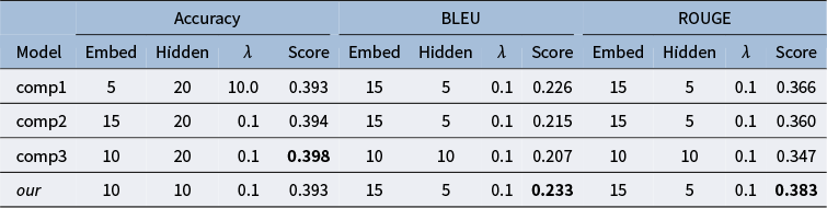
Table 2 Long description
A data table comparing four models: comp1, comp2, comp3, and our model. The table is divided into three main metric sections, each with columns for Embed, Hidden, lambda, and Score.
* Accuracy Section:
- comp1: Embed 5, Hidden 20, lambda 10.0, Score 0.393.
- comp2: Embed 15, Hidden 20, lambda 0.1, Score 0.394.
- comp3: Embed 10, Hidden 20, lambda 0.1, Score 0.398 (bold).
- our: Embed 10, Hidden 10, lambda 0.1, Score 0.393.
* B L E U Section:
- comp1: Embed 15, Hidden 5, lambda 0.1, Score 0.226.
- comp2: Embed 15, Hidden 5, lambda 0.1, Score 0.215.
- comp3: Embed 10, Hidden 10, lambda 0.1, Score 0.207.
- our: Embed 15, Hidden 5, lambda 0.1, Score 0.233 (bold).
* R O U G E Section:
- comp1: Embed 15, Hidden 5, lambda 0.1, Score 0.366.
- comp2: Embed 15, Hidden 5, lambda 0.1, Score 0.360.
- comp3: Embed 10, Hidden 10, lambda 0.1, Score 0.347.
- our: Embed 15, Hidden 5, lambda 0.1, Score 0.383 (bold).
Note: The best score for each metric is highlighted in bold.
We observe that the optimal hyperparameter configuration based on BLEU and ROUGE is the same for both our proposed function and the three competitors. However, the configuration selected based on accuracy differs from this. Given the minimal differences in accuracy and the consistency between BLEU and ROUGE, we choose the hyperparameter configuration selected by BLEU and ROUGE and use it to extract the features. That is, for the testing blocks, the extracted feature has a dimension of
$h=5$
 .
.
5.2 The best fitted T-LSTM Autoencoder model for learning blocks
Following the same procedure used for the testing blocks, we evaluate the T-LSTM Autoencoder model for the learning block fixation sequence data. For the learning blocks, we design the function
$g(\cdot )$
 as
$g(l)=1.5\exp (-0.004 l)$
as
$g(l)=1.5\exp (-0.004 l)$
 . To compare its performance, we also consider three alternative functions:
$g(l)=1$
. To compare its performance, we also consider three alternative functions:
$g(l)=1$
 (comp1),
$g(l)=1.5(\frac {l}{300}-1)^2 + 0.1$
(comp1),
$g(l)=1.5(\frac {l}{300}-1)^2 + 0.1$
 (comp2), and
$g(l)=0.5\exp (0.003 l)-0.45$
(comp2), and
$g(l)=0.5\exp (0.003 l)-0.45$
 (comp3), as illustrated in Figure A1 in the Supplementary Material. The performance of the model with different
$g(\cdot )$
(comp3), as illustrated in Figure A1 in the Supplementary Material. The performance of the model with different
$g(\cdot )$
 functions is evaluated using accuracy, BLEU score, and ROUGE score, with results presented in Table 3.
Comparison of model performance across different metrics (Accuracy, BLEU, and ROUGE) for the learning blocks, with their chosen hyperparameters

Table 3 Long description
The table is organized into three main metric sections: Accuracy, B L E U, and R O U G E. Each section includes hyperparameters for Embed, Hidden, and lambda, followed by the Score.
* comp 1: Accuracy (Embed 5, Hidden 5, lambda 0.1, Score 0.409); B L E U (Embed 5, Hidden 10, lambda 1, Score 0.139); R O U G E (Embed 5, Hidden 10, lambda 1, Score 0.268).
* comp 2: Accuracy (Embed 10, Hidden 20, lambda 0.1, Score 0.392); B L E U (Embed 15, Hidden 20, lambda 1, Score 0.073); R O U G E (Embed 5, Hidden 5, lambda 0.1, Score 0.214).
* comp 3: Accuracy (Embed 5, Hidden 10, lambda 0.1, Score 0.391); B L E U (Embed 15, Hidden 10, lambda 1, Score 0.075); R O U G E (Embed 15, Hidden 5, lambda 1, Score 0.204).
* our: Accuracy (Embed 5, Hidden 20, lambda 0.1, Score 0.400); B L E U (Embed 10, Hidden 20, lambda 0.1, Score 0.147); R O U G E (Embed 10, Hidden 20, lambda 0.1, Score 0.292).
The scores 0.147 for B L E U and 0.292 for R O U G E in the ‘our’ model row are the highest in their respective categories.
Note: The best scores for each metric are highlighted in bold.
We observe similar trends between the learning blocks and the testing blocks. First, different choices for the
$g(\cdot )$
 function show comparable results in terms of accuracy, with the highest value being 0.409 and the lowest 0.391, while showing significant variation in BLEU and ROUGE scores. Second, the function we designed achieves the best performance in BLEU (0.147) and ROUGE (0.292). Third, the optimal hyperparameter configuration based on BLEU and ROUGE is consistent for both our proposed function and comp1, whereas the configuration selected based on accuracy differs. Given the small variations in accuracy and the strong alignment between BLEU and ROUGE metrics, we use the configuration identified by BLEU and ROUGE to extract features. Specifically, for the learning blocks, the extracted features have a dimension of
$h=20$
function show comparable results in terms of accuracy, with the highest value being 0.409 and the lowest 0.391, while showing significant variation in BLEU and ROUGE scores. Second, the function we designed achieves the best performance in BLEU (0.147) and ROUGE (0.292). Third, the optimal hyperparameter configuration based on BLEU and ROUGE is consistent for both our proposed function and comp1, whereas the configuration selected based on accuracy differs. Given the small variations in accuracy and the strong alignment between BLEU and ROUGE metrics, we use the configuration identified by BLEU and ROUGE to extract features. Specifically, for the learning blocks, the extracted features have a dimension of
$h=20$
 .
.
5.3 Results for testing behavior research questions (RQ1–RQ3)
5.3.1 Hierarchical clustering results
The dendrogram and Silhouette analysis of the hierarchical clustering results using features from test blocks 1 and 2 are shown in Figure 10. The Silhouette analysis suggests an optimal cluster number of 5, where the silhouette score peaks and then plateaus with minimal variation. The dendrogram also supports this choice, with clear separation between clusters at this level. Beyond this, merging occurs at higher heights, indicating weaker cohesion within larger clusters.
(a) Hierarchical clustering dendrogram. (b) Silhouette analysis.

Figure 10 Long description
Panel a displays a hierarchical clustering dendrogram. A large vertical branch on the left descends to Cluster 1. On the right, a major branch splits into sub-branches for Cluster 2 and Cluster 3, and another sub-branch for Cluster 4 and Cluster 5. A horizontal dashed red line intersects the lower portion of the dendrogram across all five clusters. Panel b is a line graph with the y-axis labeled Silhouette score ranging from 0.65 to 0.95 and the x-axis labeled number of clusters ranging from 2 to 14. The data shows a steep linear increase from 2 to 5 clusters, followed by an asymptotic curve that plateaus near a score of 0.95. A red circle highlights the data point at 5 clusters, where the silhouette score is approximately 0.90.
5.3.2 RQ1: Interpretation of testing clusters
In Table 4, we present basic information for each cluster, including the number of observations, average accuracy, and the proportion of sequence originating from test block 1. These basic statistics highlight notable differences among the clusters. For example, Cluster 1 has the highest average accuracy (0.74), whereas Cluster 2 shows the lowest accuracy (0.59). A detailed analysis of each cluster and their corresponding problem-solving strategies is provided in the following sections.
Descriptive statistics for five testing clusters

Table 4 Long description
The table consists of six columns and four rows.
Column headers from left to right are: Empty cell, Cluster 1, Cluster 2, Cluster 3, Cluster 4, and Cluster 5.
Row 1, Number: Cluster 1 has 699, Cluster 2 has 204, Cluster 3 has 117, Cluster 4 has 154, and Cluster 5 has 213.
Row 2, Avg. acc: Cluster 1 is 0.74, Cluster 2 is 0.59, Cluster 3 is 0.68, Cluster 4 is 0.64, and Cluster 5 is 0.65.
Row 3, Prop of block 1: Cluster 1 is 68%, Cluster 2 is 22%, Cluster 3 is 26%, Cluster 4 is 41%, and Cluster 5 is 35%.
Figure 11 shows the proportion of each fixation location in each cluster. Across all clusters, the highest proportions are for “look_1” and “question,” indicating participants focus on these areas during problem-solving. All clusters have low fixation proportions for “option_correct,” suggesting less gaze effort for correct options. “Look” consistently has the lowest fixation proportions, indicating limited attention to non-key areas.
The distribution of six fixation locations for each cluster.

Figure 11 Long description
A multi-panel figure containing five pie charts labeled Cluster 1 through Cluster 5 and a legend. Each chart contains six colored segments with corresponding symbols and percentages.
Cluster 1. Red circle 8.18 percent. Blue triangle 23.08 percent. Green plus 13.19 percent. Yellow inverted triangle 26.19 percent. Purple X 9.10 percent. Orange diamond 20.25 percent.
Cluster 2. Red circle 6.19 percent. Blue triangle 31.73 percent. Green plus 12.70 percent. Yellow inverted triangle 27.99 percent. Purple X 5.78 percent. Orange diamond 15.60 percent.
Cluster 3. Red circle 5.88 percent. Blue triangle 32.18 percent. Green plus 12.36 percent. Yellow inverted triangle 26.56 percent. Purple X 6.44 percent. Orange diamond 16.58 percent.
Cluster 4. Red circle 6.64 percent. Blue triangle 26.77 percent. Green plus 13.03 percent. Yellow inverted triangle 29.86 percent. Purple X 6.92 percent. Orange diamond 16.78 percent.
Cluster 5. Red circle 7.59 percent. Blue triangle 26.40 percent. Green plus 13.94 percent. Yellow inverted triangle 26.04 percent. Purple X 6.98 percent. Orange diamond 19.05 percent.
The Action legend at the bottom-right maps symbols to labels. Red circle is look. Blue triangle is look_1. Green plus is look_2. Purple X is option_correct. Orange diamond is option_wrong. Yellow inverted triangle is question.
Cluster 1 has a relatively balanced distribution of fixations on these different locations, with moderate focus on Look_1 (23%) and Question (26%); the highest exploration of incorrect options and correct options among the five clusters. The fixation location distributions from Clusters 2 and 3 are similar, especially the proportions of Look 1 are similar and higher than the other three clusters. Cluster 4 has the highest proportion for the Question (30%) among the five clusters and relatively balanced focus on Look_1 (27%) and Option_Wrong (17%). Cluster 5 has balanced proportions between Look_1 (26%), Look_2 (14%), and Question (26%).
Table 5 provides the summary statistics for the distribution of sequence length for each cluster. Cluster 1 has the shortest average sequence length compared to the other four clusters. The remaining four clusters have similar sequence length distributions, with Cluster 2 exhibiting the longest sequence lengths among them.
Summary statistics of sequence length distribution for each cluster

Table 5 Long description
The table consists of seven columns: Cluster, Min, 1st Q, Median, Mean, 3rd Q, and Max.
* Cluster 1: Min 2.00, 1st Q 29.00, Median 48.00, Mean 53.55, 3rd Q 70.00, Max 167.00.
* Cluster 2: Min 29.00, 1st Q 96.75, Median 141.50, Mean 171.69, 3rd Q 225.00, Max 635.00.
* Cluster 3: Min 25.0, 1st Q 78.0, Median 123.0, Mean 142.6, 3rd Q 178.0, Max 404.0.
* Cluster 4: Min 4, 1st Q 80.25, Median 115.00, Mean 135.44, 3rd Q 176.50, Max 543.00.
* Cluster 5: Min 21.0, 1st Q 75.0, Median 117.0, Mean 134.9, 3rd Q 161.0, Max 458.0.
The adjusted transition matrix for each cluster in Figure 12 highlights how transition probabilities deviate from the overall pattern. Positive values (red) indicate transitions that occur more frequently within the cluster compared to the overall data, while negative values (purple) indicate transitions that occur less frequently. Cluster 1 shows fewer self-transitions, suggesting participants avoid focusing on the same areas or lingering too long. Cluster 2 has more self-transitions (L1–L1, Q–Q) and fewer L1–L2 transitions, indicating less systematic exploration. Cluster 3 mirrors Cluster 2 but with fewer transitions from Wrong to Q, Q to Wrong, and Q to Correct, suggesting a more focused problem-solving approach. Cluster 4’s pattern is similar to the overall average, with slight increases in transitions like L to L1 and Q to Q, reflecting a more cautious strategy. Slight decreases in transitions like L to Q and Correct to Wrong suggest reduced guessing or incorrect answers. Cluster 5 resembles Cluster 4 but shows fewer repetitive movements, such as L1 to L1 and Correct to Q, and more transitions from Correct to Wrong.
The adjusted transition matrix for five clusters.

Figure 12 Long description
A multi-panel figure with five heatmaps arranged in two rows. The top row contains Cluster 1, Cluster 2, and Cluster 3. The bottom row contains Cluster 4 and Cluster 5.
Each heatmap shares the same axes. The vertical Y axis is labeled From Action and the horizontal X axis is labeled To Action. The categories on both axes from bottom to top and left to right are L, L sub 1, L sub 2, Q, O underscore Corr, and O underscore Wro.
A color scale legend on the right indicates Probability values ranging from negative 0.10 in dark blue to 0.10 in dark red, with white representing 0.00.
* Cluster 1 shows strong negative probabilities (blue) for transitions from L sub 1 and L to L sub 1, and from Q to Q.
* Cluster 2 shows positive probabilities (red) for transitions from L and L sub 1 to L sub 1, and from Q to Q.
* Cluster 3 shows a strong positive probability (dark red) for the transition from L to L sub 1 and a negative probability (blue) for L to L.
* Cluster 4 shows a more neutral distribution with light blue and light red patches, including a negative probability for O underscore Corr to O underscore Wro.
* Cluster 5 shows light blue negative probabilities for transitions from L sub 1 and L sub 2 to L sub 1, and a positive probability for O underscore Corr to O underscore Wro.
Based on the above analysis, we interpret the five testing clusters as representing five distinct problem-solving strategies, summarized in Table 6.
Problem solving (PS) behaviors interpretation

Table 6 Long description
The table consists of two columns titled Cluster and Characteristics.
* Row 1: T C 1 (Quick Navigation P S) is characterized as exploratory and less focused on screen.
* Row 2: T C 2 (Example-Driven P S) is characterized as highly relying on example questions and the choices they choose.
* Row 3: T C 3 (Targeted P S) is characterized by focused and deliberate engagement with specific areas.
* Row 4: T C 4 (Less decisive P S) is characterized by moderate change, with slightly cautious tendencies.
* Row 5: T C 5 (Balanced P S) is characterized by a balance of explorations and answering questions.
5.3.3 RQ2: The change of problem-solving strategies
Figure 13 shows two mosaic plots comparing five problem-solving strategies and seven item types across two test blocks. In test block 1 (before learning interventions), participants primarily use the quick navigation strategy (Cluster 1) for easier one-direction rotation items (
$x90$
 ,
$y90$
,
$y90$
 ,
$x180$
,
$x180$
 ,
$y180$
,
$y180$
 ). This strategy decreases as the items become more complex with two-direction rotations (
$x180y90$
). This strategy decreases as the items become more complex with two-direction rotations (
$x180y90$
 ,
$x90y90$
,
$x90y90$
 ,
$x90y180$
,
$x90y180$
 ), indicating greater difficulty. The targeted strategy (Cluster 3) is less common but increases slightly for more difficult two-direction rotations. The remaining strategies (Clusters 2, 4, and 5) show varying patterns. The
$G^2$
), indicating greater difficulty. The targeted strategy (Cluster 3) is less common but increases slightly for more difficult two-direction rotations. The remaining strategies (Clusters 2, 4, and 5) show varying patterns. The
$G^2$
 test reveals a significant dependence between the testing cluster and item type in test block 1 (
$G^2(24)=159.15,\ p<0.001$
test reveals a significant dependence between the testing cluster and item type in test block 1 (
$G^2(24)=159.15,\ p<0.001$
 ), with Cramer’s V of 0.216, indicating a moderate association.
The mosaic plot of contingency table between item type and testing cluster in two tests.

Figure 13 Long description
A two-panel mosaic plot. Each panel has item type on the horizontal axis and testing cluster on the vertical axis. The vertical axis is numbered 1 to 5 from top to bottom, corresponding to a color gradient from red (1) to orange (2), gold (3), yellow (4), and pale yellow (5).
Panel 1 (Test 1):
- The horizontal axis lists item types: x 1 8 0, x 1 8 0 y 9 0, x 9 0, x 9 0 y 1 8 0, x 9 0 y 9 0, y 1 8 0, and y 9 0.
- Cluster 1 (red) dominates almost all item types, occupying the majority of the vertical space.
- Clusters 2 through 5 are compressed at the bottom for most categories, appearing as thin slivers or small blocks.
Panel 2 (Test 2):
- The horizontal axis uses the same item types as Test 1.
- The distribution is much more varied compared to Test 1.
- Cluster 1 (red) remains large in x 9 0, x 9 0 y 9 0, and y 1 8 0, but is significantly smaller in x 1 8 0 y 9 0 and x 9 0 y 1 8 0.
- Clusters 2 (orange), 3 (gold), 4 (yellow), and 5 (pale yellow) occupy much larger, more distinct rectangular blocks across all item types, indicating a more even distribution of testing clusters in Test 2.
We observed a marked decrease for quick navigation (Cluster 1) in test block 2 compared to test block 1, especially on more difficult items (
$x180y90$
 ,
$x90y180$
,
$x90y180$
 ), suggesting participants have moved away from a stepwise exploratory approach after learning interventions. The other four clusters all increase across different types of items. The
$G^2$
), suggesting participants have moved away from a stepwise exploratory approach after learning interventions. The other four clusters all increase across different types of items. The
$G^2$
 statistics show a significant dependence between testing cluster in test block 2 and item type at significance level of 0.05,
$G^2(24)=184.35,\ p<0.001$
statistics show a significant dependence between testing cluster in test block 2 and item type at significance level of 0.05,
$G^2(24)=184.35,\ p<0.001$
 . The Cramer’s V is 0.249, indicating a moderate association.
5.3.4 RQ3: The relationship between problem-solving strategies and score
The GLMM results are summarized in Table 7. Quick navigation strategy (Cluster 1) serves as the reference group, with test takers using this strategy showing the highest probability of correct responses after controlling for covariates. Both Example Driven (Cluster 2) and Less Decisive (Cluster 4) strategies have significantly lower probabilities of correct responses compared to Quick Navigation. No significant difference in response probability is found between Quick Navigation (Cluster 1) and Targeted strategy (Cluster 3), suggesting similar performance levels. Although not significant, the Balanced strategy (Cluster 5) shows a slightly lower probability of correct responses than Quick Navigation, implying that it may not consistently lead to correct outcomes. More complex items (item_type = 1) significantly reduce correct response probabilities, highlighting the difficulty of items requiring two skills. Questions in test block 2 (after intervention) show significantly higher probabilities of correct responses than test block 1.
Generalized linear mixed model results

Table 7 Long description
The table consists of five columns: Parameter, Estimate, Std. error, z value, and Pr(>|z|).
* (Intercept): Estimate 1.6821, Std. error 0.1840, z value 9.140, p value less than 2e-16.
* cls2: Estimate minus 0.6456, Std. error 0.2502, z value minus 2.581, p value 0.009856.
* cls3: Estimate minus 0.1737, Std. error 0.2965, z value minus 0.586, p value 0.558150.
* cls4: Estimate minus 0.5588, Std. error 0.2540, z value minus 2.200, p value 0.027823.
* cls5: Estimate minus 0.2745, Std. error 0.2363, z value minus 1.161, p value 0.245440.
* item_type2: Estimate minus 1.3279, Std. error 0.1743, z value minus 7.618, p value less than 0.001.
* block_id1: Estimate 0.5451, Std. error 0.1644, z value 3.317, p value 0.000911.
5.4 Results for learning behavior research questions (RQ4–RQ6)
5.4.1 Hierarchical clustering results
The extracted features from fixation sequences in learning blocks 1 and 2 have a high dimensionality of 20, which can make distance calculations for hierarchical clustering less meaningful due to the curse of dimensionality. To address this, we apply principal component analysis (PCA) to reduce dimensionality, removing noise and redundancy for more efficient clustering and improved interpretability. Based on the Scree plot in Figure 14(a), we identify three principal components as optimal, as the “elbow” in the plot shows that these components capture most of the variance, with additional components explaining minimal variance. Hierarchical clustering is then performed using these three components.
(a) Scree plot showing the percentage of variance explained by each principal component. (b) Hierarchical clustering dendrogram. (c) Silhouette analysis.

Figure 14 Long description
Panel a is a line graph titled Scree plot. The x-axis is labeled Principal Component from 0 to 20. The y-axis is labeled Percentage of Variance Explained from 0 to 30. The data shows a sharp exponential decay starting near 35 percent for component 1 and leveling off near zero by component 10. A red circle highlights the elbow point at component 3.
Panel b is a hierarchical clustering dendrogram. It shows a branching tree structure with four main groups labeled Cluster 1, Cluster 2, Cluster 3, and Cluster 4 at the bottom. A horizontal dashed red line intersects the vertical branches to indicate the clustering threshold.
Panel c is a line graph titled Silhouette analysis. The x-axis is labeled number of clusters from 2 to 14. The y-axis is labeled Silhouette score from 0.60 to 0.85. The curve increases from 0.58 at 2 clusters to a peak of approximately 0.86 at 11 clusters before declining. A red circle highlights the data point at 4 clusters, which has a score of approximately 0.72.
The results of the Silhouette analysis and dendrogram are shown in Figure 14(b) and (c). The Silhouette analysis shows a significant increase in the score when the number of clusters rises from two to three. Adding more clusters continues to improve the score, but at a slower rate, up to nine clusters. However, nine clusters reduce interpretability. Based on the dendrogram, four clusters are identified as the most suitable, as they are well-separated and avoid the weaker cohesion seen with further merging.
5.4.2 RQ4: Interpretation of learning clusters
The descriptive statistics for each learning cluster, including the number of observations, average accuracy, and the proportion of data from learning block 1, are summarized in Table 8. The fixation sequence in Clusters 1 and 2 has higher response accuracy than Clusters 3 and 4, and learning block 1 is dominated by Clusters 1 and 2.
Descriptive statistics for four learning clusters

Table 8 Long description
The table consists of five columns and four rows. The first column lists the metrics, while columns two through five are labeled Cluster 1, Cluster 2, Cluster 3, and Cluster 4.
* Row 1 (Number): Cluster 1 has 338, Cluster 2 has 489, Cluster 3 has 212, and Cluster 4 has 350.
* Row 2 (Avg. acc): Cluster 1 is 0.84, Cluster 2 is 0.87, Cluster 3 is 0.67, and Cluster 4 is 0.67.
* Row 3 (Prop of learning block 1): Cluster 1 is 59%, Cluster 2 is 78%, Cluster 3 is 15%, and Cluster 4 is 24%.
Figure 15 documents the distributions of eye fixation locations for each cluster. Cluster 1 shows a balanced approach, distributing attention across the “Question” (26.82%), the example object’s initial position (“Look 1,” 25.90%), and other elements like “Look 2” (14.96%) and “Option Wrong” (16.09%). They balance revisiting the problem with analyzing both correct and incorrect options. Cluster 2 exhibits a fairly even distribution, with notable focus on “Look 1” (20.29%), “Option Wrong” (21.20%), and “Question” (26.79%). Participants likely use feedback to assess why their previous solution was incorrect, with high attention to “Option Wrong” indicating analysis of earlier mistakes. Cluster 3 focuses heavily on the example object’s initial position (“Look 1,” 32.68%), with less attention to answer options (“Option Wrong” 14.80%, “Option Correct” 5.17%). They spend significant time on the “Question” (26.40%) and some on “Look 2” (13.61%), relying primarily on the example setup to reanalyze the task, with limited focus on validating or correcting their solution. Cluster 4 focuses most on the “Question” (31.12%), indicating strong engagement with the task. Their attention to the example object (“Look 1,” 24.27%; “Look 2,” 12.21%) and options (“Option Wrong” 17.82%; “Option Correct” 6.78%) is lower, suggesting they prioritize applying feedback to the task rather than analyzing object transitions or comparing previous solutions.
The distribution of six fixation locations for each cluster.

Figure 15 Long description
A four-panel set of pie charts. A legend on the right maps symbols to actions: red circle for look, blue triangle for look_1, green plus for look_2, purple X for option_correct, orange diamond for option_wrong, and yellow inverted triangle for question.
* Cluster 1 (top-left): look 7.23%, look_1 25.90%, look_2 14.96%, question 26.82%, option_correct 8.99%, and option_wrong 16.09%.
* Cluster 2 (top-right): look 8.70%, look_1 20.29%, look_2 12.68%, question 26.79%, option_correct 10.34%, and option_wrong 21.20%.
* Cluster 3 (bottom-left): look 7.34%, look_1 32.68%, look_2 13.61%, question 26.40%, option_correct 5.17%, and option_wrong 14.80%.
* Cluster 4 (bottom-right): look 7.80%, look_1 24.27%, look_2 12.21%, question 31.12%, option_correct 6.78%, and option_wrong 17.82%.
In all clusters, the question and look_1 actions represent the largest segments of fixation distribution.
Table 9 summarizes the distribution of sequence lengths for each cluster. Cluster 1 has short sequences, with a maximum of 331 fixations. Most sequences range from the 1st quartile (26.0) to the 3rd quartile (78.0), indicating brief task engagement. Cluster 2 shows the shortest sequences among four clusters, with a maximum of 124 fixations. Most sequence lengths range from 22.0 (1st quartile) to 48.0 (3rd quartile), reflecting minimal engagement with task components. Cluster 3 has the longest sequences, with a maximum of 555 fixations. Most sequences range from 71.75 (1st quartile) to 160.25 (3rd quartile), suggesting extensive engagement with the task. Cluster 4 has moderate sequence lengths, with a maximum of 451 fixations. Most sequences range from 54.0 (1st quartile) to 104.75 (3rd quartile), indicating balanced engagement—participants process the task meaningfully without the exhaustive focus seen in Cluster 3.
Summary statistics of sequence length distribution for each cluster

Table 9 Long description
The table consists of seven columns: Cluster, Min, 1st Q, Median, Mean, 3rd Q, and Max.
* Cluster 1: Min 2.00, 1st Q 26.00, Median 44.50, Mean 62.33, 3rd Q 78.00, Max 331.00.
* Cluster 2: Min 2.00, 1st Q 22.00, Median 33.00, Mean 36.72, 3rd Q 48.00, Max 124.00.
* Cluster 3: Min 21.00, 1st Q 71.75, Median 106.00, Mean 129.09, 3rd Q 160.25, Max 555.00.
* Cluster 4: Min 16.00, 1st Q 54.00, Median 71.50, Mean 88.73, 3rd Q 104.75, Max 451.00.
The adjusted transition matrices in Figure 16 reflect the dynamic characteristics of transitions between different actions for each cluster. Compared to the overall transition pattern, Cluster 1 shows a higher likelihood of transitioning from Option Wrong to Correct, L2 to L1, and Correct to L1, while transitions from L to L1, L2 to L1, Correct to Wrong, and Q to Q decrease. Participants in this cluster focus on exploring multiple task components after receiving feedback, especially incorrect options, reflecting a reflective approach to error evaluation. Cluster 2 has significantly fewer self-transitions (L1 to L1, L2 to L2, Q to Q, and Wrong to Wrong) and a higher likelihood of transitioning from Option Correct to Option Wrong, Wrong to Correct, L1 to L2, Q to Option Correct, and L1 to Q. This strategy centers on feedback and its connection to the example’s rotation process, with less focus on the new task, indicating time spent consolidating understanding of previous mistakes. Cluster 3 shows a higher likelihood of staying in L1, transitioning from L to L1, and Q to Q, with slightly fewer transitions from L1 to L2, L to Q, Q to Correct, Wrong to Correct, and Correct to Wrong. Cluster 4’s transition pattern is close to the overall average, with slightly higher chances for Q to Q, Wrong to Wrong, and Wrong to Q, and a slightly lower chance for Wrong to Correct.
The adjusted transition matrix for four clusters.

Figure 16 Long description
The figure contains four heatmaps labeled Adjusted Transition Matrix for Cluster 1 through Cluster 4. All panels share the same axes. The y-axis is labeled From Action and the x-axis is labeled To Action. Both axes contain six categories: L, L sub 1, L sub 2, Q, O underscore Corr, and O underscore Wro. A color scale on the right indicates Probability, ranging from negative 0.10 in dark blue to 0.10 in dark red, with white representing 0.00.
* Top-left, Cluster 1: Shows high positive probability (red) for transitions from O underscore Wro to O underscore Corr and from L to L sub 2. Negative probability (blue) is seen for transitions from L to L sub 1.
* Top-right, Cluster 2: Displays a strong diagonal trend of negative probability (blue) from L sub 1 to L sub 1, L sub 2 to L sub 2, and Q to Q. High positive probability (red) is seen for transitions from O underscore Corr to O underscore Wro.
* Bottom-left, Cluster 3: Features a prominent vertical band of high positive probability (red) in the L sub 1 column, particularly from actions L and L sub 1. Negative probability (blue) is scattered in the O underscore Wro and Q columns.
* Bottom-right, Cluster 4: Shows a more diffused pattern with light red concentrations for transitions from L to L and Q to Q, indicating lower overall variance compared to the other clusters.
The above analysis suggests that the four clusters represent distinct learning strategies based on participants’ eye fixation patterns after receiving feedback on their solution. These patterns reveal how participants process feedback, evaluate their original solution, and learn from the example in the spatial rotation task. Table 10 summarizes our interpretations of the four learning clusters.
Learning behaviors interpretation

Table 10 Long description
The table consists of two columns: Cluster and Characteristics.
* Cluster L C 1 (Reflective exploring): Characteristics include actively exploring and evaluating errors; using feedback to analyze both the problem and example components; and maintaining a balance between reflection and application.
* Cluster L C 2 (Feedback-focused): Characteristics include prioritizing understanding why a solution was incorrect; revisiting and analyzing example transitions; and minimal engagement with new tasks.
* Cluster L C 3 (Deep process-oriented): Characteristics include engaging deeply with the example rotation process and feedback; and focusing on understanding the rotation principles.
* Cluster L C 4 (Task-oriented): Characteristics include being task-oriented and action-driven; and engaging with feedback to inform immediate problem-solving efforts.
5.4.3 RQ5: Association between learning behavior and item type
Figure 17 shows two mosaic plots comparing four types of learning behaviors and different item types across two learning blocks. Block 1 consists mainly of one-direction rotation items, which are easier to visualize. Participants primarily use reflective (Cluster 1) or feedback-focused (Cluster 2) strategies after receiving feedback. Some also use the other two strategies for solving rotations like
$x180$
 ,
$x90y90$
,
$x90y90$
 , and
$y180$
, and
$y180$
 . Block 2 introduces more complex two-direction rotations, where we observe a significant increase in deep process-oriented (Cluster 3) and task-oriented (Cluster 4) strategies. The
$\chi ^2$
. Block 2 introduces more complex two-direction rotations, where we observe a significant increase in deep process-oriented (Cluster 3) and task-oriented (Cluster 4) strategies. The
$\chi ^2$
 tests for both blocks show that learning strategy is significantly related to item type:
$G^2(12)=124.36$
tests for both blocks show that learning strategy is significantly related to item type:
$G^2(12)=124.36$
 ,
$p<0.001$
,
$p<0.001$
 , Cramer’s V = 0.219 for Block 1 and
$G^2(18)=112.03$
, Cramer’s V = 0.219 for Block 1 and
$G^2(18)=112.03$
 ,
$p<0.001$
,
$p<0.001$
 , Cramer’s V = 0.214 for Block 2.
The mosaic plot of the two contingency tables.

Figure 17 Long description
The image consists of two side-by-side mosaic plots.
Left Panel (L B 1):
The horizontal axis lists five categories: x 1 8 0, x 9 0, x 9 0 y 9 0, y 1 8 0, and y 9 0. The vertical axis represents learning clusters 1, 2, 3, and 4.
- Cluster 1 (red) is largest in x 1 8 0, x 9 0, and y 1 8 0.
- Cluster 2 (orange) dominates x 1 8 0, x 9 0, y 1 8 0, and y 9 0.
- Cluster 3 (yellow) and Cluster 4 (pale yellow) are significantly smaller across most categories, appearing as thin bands at the bottom of the columns.
Right Panel (L B 2):
The horizontal axis lists seven categories: x 1 8 0, x 1 8 0 y 9 0, x 9 0, x 9 0 y 1 8 0, x 9 0 y 9 0, y 1 8 0, and y 9 0. The vertical axis represents the same four learning clusters.
- Cluster 1 (red) is most prominent in x 1 8 0, x 9 0 y 1 8 0, and y 1 8 0.
- Cluster 2 (orange) and Cluster 3 (yellow) show a more even distribution compared to L B 1, with Cluster 3 being particularly large in x 1 8 0 y 9 0 and y 1 8 0.
- Cluster 4 (pale yellow) occupies the largest area at the bottom of every column, indicating a higher frequency of this cluster in the L B 2 dataset compared to L B 1.
5.4.4 RQ6: How learning behaviors impact the testing behaviors
Since test block 2 follows directly after learning block 2, we construct another 4 by 5 contingency table (Figure 18) to examine the relationship between participants’ primary learning behaviors in learning block 2 and their primary problem-solving strategies in test block 2. It’s important to note that each participant may exhibit different learning and testing behaviors across these blocks. The major strategy for each participant is defined as the one they use most frequently when solving or learning a question.
The plot of contingency table between LB2 cluster mode and TB2 cluster mode.

Figure 18 Long description
The mosaic plot is divided into four main vertical columns representing L B 2 cluster modes 1, 2, 3, and 4. The width of the columns increases from left to right. Within each column, rectangles are stacked vertically to represent T B 2 cluster modes 1 through 5, colored in a gradient from red at the top to pale yellow at the bottom.
* Column 1 (L B 2 mode 1): Dominated by a large red rectangle for T B 2 mode 1 at the top, followed by a smaller orange rectangle for mode 2, and a medium pale yellow rectangle for mode 5 at the base.
* Column 2 (L B 2 mode 2): Features a very tall red rectangle for T B 2 mode 1, with very thin slivers for modes 2, 3, and 4, and a small yellow rectangle for mode 5.
* Column 3 (L B 2 mode 3): Contains a medium red rectangle for mode 1, a large orange rectangle for mode 2, and thin yellow/pale yellow bands for modes 3, 4, and 5.
* Column 4 (L B 2 mode 4): The widest column, showing a large red square for mode 1, a medium orange rectangle for mode 2, and three thin horizontal bands in yellow and pale yellow for modes 3, 4, and 5.
We observe that participants who primarily exhibit reflective exploring behavior (LC1) in learning block 2 are more likely to use Quick Navigation (TC1) and Balanced Problem Solving (TC5) strategies in test block 2. Participants with a feedback-focused learning behavior (LC2) tend to favor Quick Navigation (TC1). Those demonstrating a deep, process-oriented learning behavior (LC3) are more likely to use Example-Driven (TC2) strategy. Finally, participants with a task-oriented learning behavior (LC4) are more likely to use Quick Navigation (TC1), Example-Driven (TC2), and Balanced (TC5) problem-solving strategies. The association between these two types of clusters is statistically significant, with a moderate strength of association,
$G^2(12) = 23.33$
 ,
$p = 0.03$
,
$p = 0.03$
 , and Cramer’s
$V = 0.306$
, and Cramer’s
$V = 0.306$
 .
.
6 Conclusion and discussion
6.1 Contributions of this work
The major methodological contribution of this work is the T-LSTM Autoencoder framework, which extracts features from unstructured data with temporal and sequential dependencies. Our proposed T-LSTM Autoencoder differs from the original T-LSTM models in several key ways. First, our approach uses two time signals as inputs. Unlike prior models that only use elapsed time between events
$(\Delta \mathrm {t})$
 , we feed both elapsed time and event durations into the network by constructing the input
$X_i= \left [E_i, \ell _i, d_i\right ]$
, we feed both elapsed time and event durations into the network by constructing the input
$X_i= \left [E_i, \ell _i, d_i\right ]$
 , where
$E_i$
, where
$E_i$
 are action embeddings,
$\ell _i$
are action embeddings,
$\ell _i$
 elapsed times, and
$d_i$
elapsed times, and
$d_i$
 durations. Second, we employ a data-driven choice of the time-decay
$g(\cdot )$
durations. Second, we employ a data-driven choice of the time-decay
$g(\cdot )$
 guided by empirical transition patterns, whereas Baytas et al. (Reference Baytas, Xiao, Zhang, Wang, Jain and Zhou2017) predefine this function, which may lead to the loss of important information present in real data. Third, we have a multi-target reconstruction objective. We jointly reconstruct actions and both time sequences using
$L=L_{\mathrm {CE}}+\lambda L_{\mathrm {MSE}}$
guided by empirical transition patterns, whereas Baytas et al. (Reference Baytas, Xiao, Zhang, Wang, Jain and Zhou2017) predefine this function, which may lead to the loss of important information present in real data. Third, we have a multi-target reconstruction objective. We jointly reconstruct actions and both time sequences using
$L=L_{\mathrm {CE}}+\lambda L_{\mathrm {MSE}}$
 , which regularizes latent features to capture what happened and when/how long. Finally, we discuss how to select hyperparameters and the weight function
$g(.)$
, which regularizes latent features to capture what happened and when/how long. Finally, we discuss how to select hyperparameters and the weight function
$g(.)$
 through a three-way evaluation based on various evaluation metrics. Results in Sections 5.1 and 5.2 demonstrate the advantages of incorporating time duration and elapsed time to improve the reconstruction of categorical fixation sequences.
While primarily illustrated with an eye-tracking dataset, our feature extraction method can be applied to any sequential data with temporal and interdependent structures, such as process and log data (e.g., Bergner & von Davier, Reference Bergner and von Davier2019; Chen, Reference Chen2020; Fang & Ying, Reference Fang and Ying2020; Greiff et al., Reference Greiff, Wüstenberg, Holt, Goldhammer and Funke2013; He et al., Reference He, von Davier and Han2016, Reference He, Shi and Tighe2023; LaMar, Reference LaMar2018; Liu et al., Reference Liu, Liu and Li2018; Qiao & Jiao, Reference Qiao and Jiao2018; Tang, Reference Tang2023; Ulitzsch et al., Reference Ulitzsch, He, Ulitzsch, Molter, Nichterlein, Niedermeier and Pohl2021; Ulitzsch, Ulitzsch, et al., Reference Ulitzsch, Ulitzsch, He and Lüdtke2023). The evaluation framework presented here can assist researchers in selecting the best Autoencoder model for their specific applications. For instance, in our case, where the goal is to reconstruct the eye-fixation sequence using time information (duration and elapsed time), the
$\lambda $
 parameter in the loss function (15) is set within a small range. For applications where time information plays a more significant role, a larger
$\lambda $
parameter in the loss function (15) is set within a small range. For applications where time information plays a more significant role, a larger
$\lambda $
 can be used.
The additional methodological contribution is demonstrating how different statistical tools can be leveraged to interpret feature extraction results in the context of educational questions. Features extracted from process data are often difficult to interpret, so we use a set of statistical tools to summarize patterns and investigate the associations between variables derived from these features. The results from these analyses address key educational questions, such as evaluating the effectiveness of test questions in assessing participants’ spatial rotation skills (examining changes in testing behaviors (E1.2) and their association with test scores (E1.3)) and the effectiveness of learning interventions in improving those skills (exploring the association between learning interventions and testing behaviors (E2.3)). These findings also have implications for the development of new psychometric models and the design of learning programs. For example, the current learning program provides the same test questions and interventions to all participants. However, results from this study suggest that participants employ different problem-solving strategies and learning behaviors, which are significantly related to specific types of questions. Based on these findings, an adaptive learning program could be developed, tailored to individual testing and learning behaviors, to improve overall learning efficiency.
6.2 Future directions
Our proposed two-component DAK can be further developed through the following perspectives. First, as one of the reviewers mentioned that, it is possible to extend our work to learn the decay coefficient
$\alpha $
 adaptively during training rather than pre-specifying it. This would allow the model to automatically discover the most appropriate temporal decay rate for different datasets.
Second, we can strengthen our current T-LSTM framework by using some complementary techniques in other T-LSTM models. For example, Nguyen et al. (Reference Nguyen, Chatterjee, Weinzierl, Schwinn, Matzner and Eskofier2021) retain the T-LSTM cell but introduce cost-sensitive learning to address class imbalance. Our objective could be extended analogously with class-weighting to handle imbalanced action distributions. Zhang (Reference Zhang2019) proposes an attention-based T-LSTM that aggregates multiple past states with temporal decay. A similar temporal-attention module could be integrated into our encoder–decoder framework to emphasize salient events.
As suggested by one reviewer, we have conducted a small preliminary experiment with an attention-based autoencoder (Appendix B of the Supplementary Material). Results show that with our current dataset size and model scale, Transformer architectures did not perform competitively compared to LSTM-based approaches. This result is consistent with the broader literature indicating that attention-based models typically require both larger model capacity and substantially larger training corpora to realize their full potential (Brown et al., Reference Brown, Mann, Ryder, Subbiah, Kaplan, Dhariwal, Neelakantan, Shyam, Sastry, Askell, Agarwal, Herbert-Voss, Krueger, Henighan, Child, Ramesh, Ziegler, Wu, Winter and Amodei2020; Haque et al., Reference Haque, Debnath, Yasmin, Mahmud and Ngu2024; Kaplan et al., Reference Kaplan, McCandlish, Henighan, Brown, Chess, Child, Gray, Radford, Wu and Amodei2020). Nevertheless, attention mechanisms remain a promising avenue for modeling eye-tracking sequences, particularly given their ability to capture both local dependencies and long-range interactions. Future work could explore scaling up Transformer architectures, adopting relative or learned positional encodings tailored for sequential fixation data, and leveraging larger or pretraining datasets (e.g., synthetic or cross-task gaze corpora). Such extensions may enable attention-based models to complement or even surpass recurrent architectures in this domain.
Supplementary material
The supplementary material for this article can be found at https://doi.org/10.1017/psy.2026.10096.
AI statement
The author utilized ChatGPT5 to help with manuscript writing process. Generative artificial intelligence was used to rephrase the authors’ original written context, which is mainly for language polishing purposes. The authors reviewed the created content produced by this generative AI Tool and assert that the content within this document is factually accurate and free of plagiarism. The authors take full responsibility for the submitted document.
Funding statement
This research was partially supported by NSF SES-2243044 and SES-2051198.
Competing interests
The authors declare that they have no competing interests.
Ethical standards
The authors declared no potential competing interests with respect to the research, authorship, and/or publication of this article. This research does not involve human participants and/or animals.

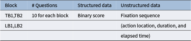
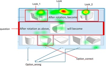
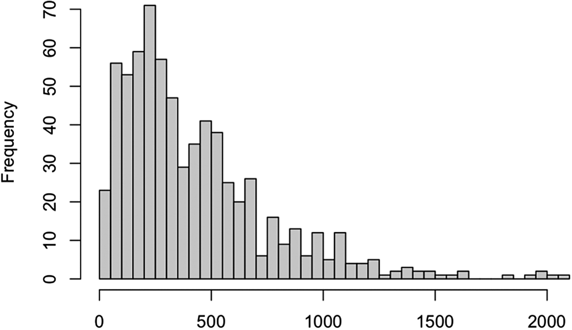
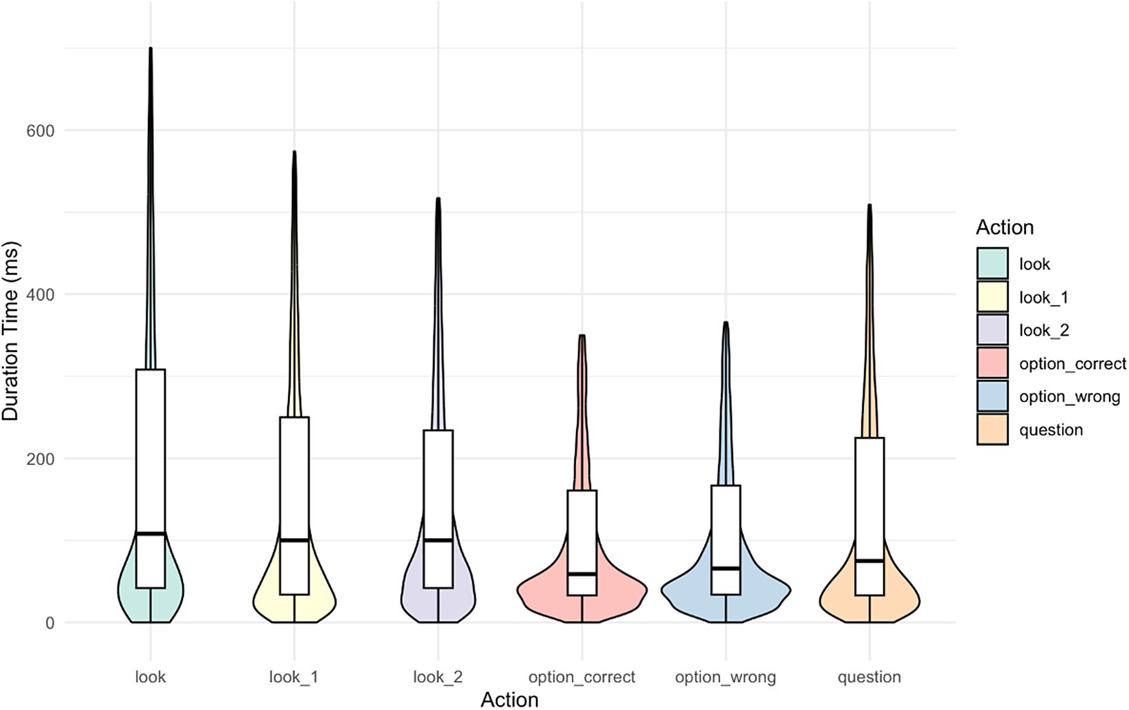
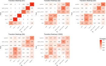
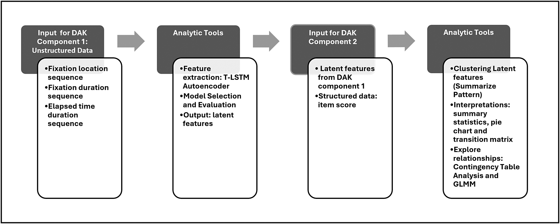
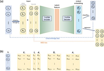


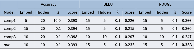
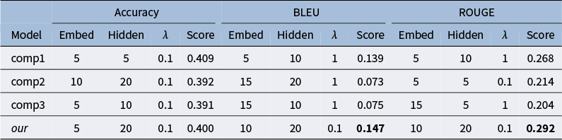
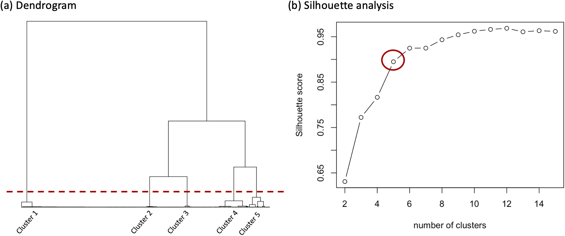
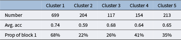

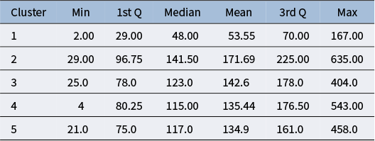

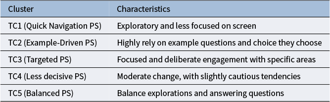
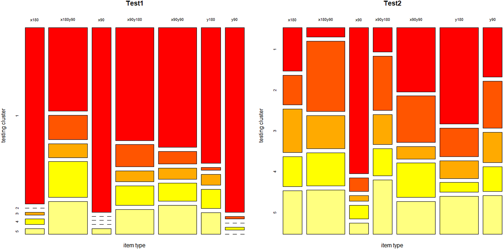
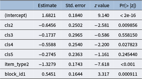
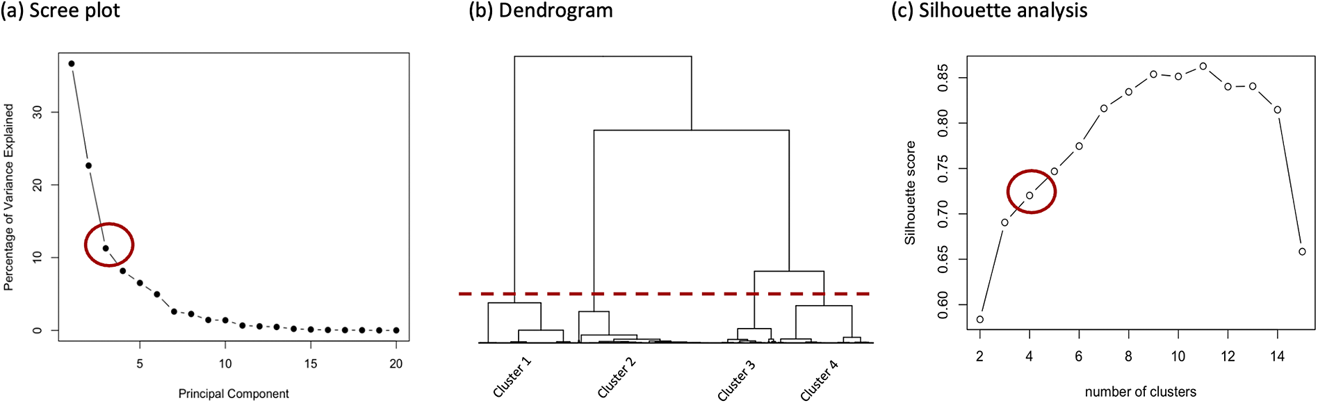
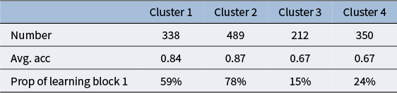
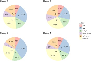
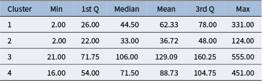

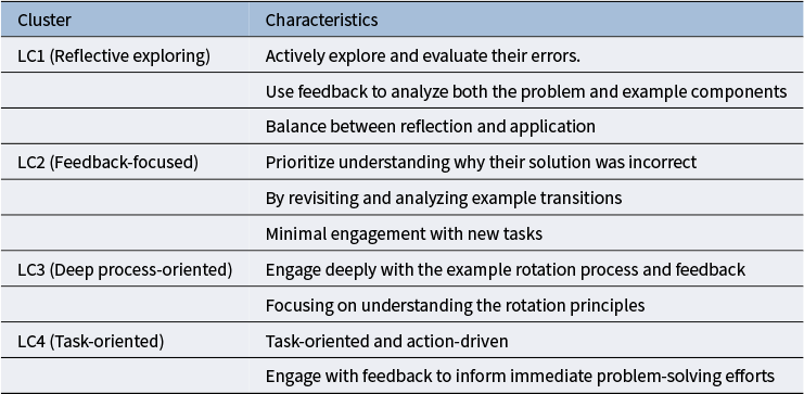
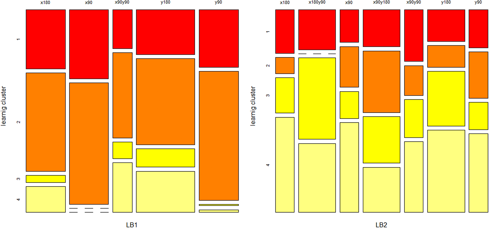
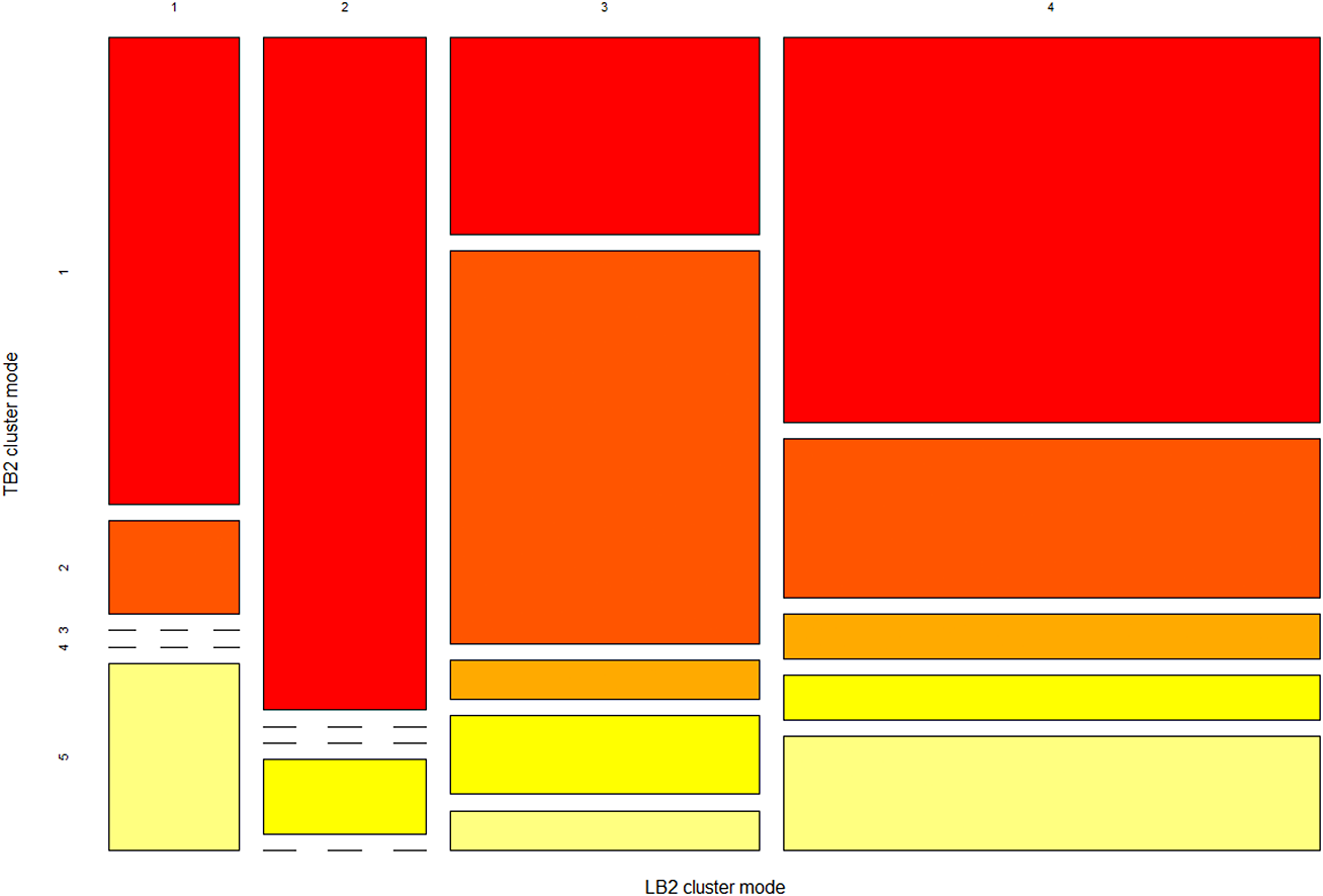


 Open access

