





1 Introduction
1.1 Background—Tennenbaum’s theorem
It is a well-known result of Tennenbaum (see, e.g., [Reference Kaye10]) that
$\mathsf {PA}$
 , the first-order theory of Peano Arithmetic, does not admit any nonstandard computable model. In fact, in every nonstandard model of
$\mathsf {PA}$
, the first-order theory of Peano Arithmetic, does not admit any nonstandard computable model. In fact, in every nonstandard model of
$\mathsf {PA}$
 , neither addition nor multiplication is computable. Generalizations of this theorem can be found in the literature, including versions of it for weaker fragments of
$\mathsf {PA}$
, neither addition nor multiplication is computable. Generalizations of this theorem can be found in the literature, including versions of it for weaker fragments of
$\mathsf {PA}$
 [Reference Wilmers20], alternative operations [Reference Schmerl19], and finite set theory [Reference Godziszewski and Hamkins7, Reference Mancini and Zambella15], to name a few. However, all of these approaches and variations appear to depend heavily on the specificities of the chosen signature. This was observed by Pakhomov, who in 2022 [Reference Pakhomov18] constructed a theory that is definitionally equivalent to
$\mathsf {PA}$
[Reference Wilmers20], alternative operations [Reference Schmerl19], and finite set theory [Reference Godziszewski and Hamkins7, Reference Mancini and Zambella15], to name a few. However, all of these approaches and variations appear to depend heavily on the specificities of the chosen signature. This was observed by Pakhomov, who in 2022 [Reference Pakhomov18] constructed a theory that is definitionally equivalent to
$\mathsf {PA}$
 (see Definition 1.2 below) for which there is a computable nonstandard model. This shows that Tennenbaum’s theorem really is reliant on the choice of signature.
In this article, we extend Pakhomov’s construction to the stronger theories obtained by adding to
$\mathsf {PA}$
 all true
$\Pi _{n}$
all true
$\Pi _{n}$
 sentences, for fixed values of n (Theorem 4.5). In the process, we obtain a general theorem for strong jump inversion (Theorem 2.6) and show that this theorem can be used to establish multiple other results already present in the literature (Section 3).
Definition 1.1 (Definitional extension)
Let T be a theory over a signature
$\mathcal {L}$
 . A definitional extension of T is a theory
$S\supseteq T$
. A definitional extension of T is a theory
$S\supseteq T$
 , over a signature
$\mathcal {L}'\supseteq \mathcal {L}$
, over a signature
$\mathcal {L}'\supseteq \mathcal {L}$
 , such that
-
• every theorem of S that only uses symbols from the signature $\mathcal {L}$
 is also a theorem of T, and
 -
• every symbol of $\mathcal {L}'\setminus \mathcal {L}$
is S-definable in terms of symbols in
$\mathcal {L}$
. For example, if P is any predicate symbol in
$\mathcal {L}'$
, there is an
$\mathcal {L}$
-formula
$\varphi $
such that $$\begin{align*}S\vdash(\forall\vec{x})(P(\vec{x})\leftrightarrow\varphi(\vec{x})), \end{align*}$$and a similar statement holds for function symbols.


Definition 1.2 (Definitional equivalence)
Let
$T_{1}$
 and
$T_{2}$
and
$T_{2}$
 be two theories, whose signatures
$\mathcal {L}_{1}$
be two theories, whose signatures
$\mathcal {L}_{1}$
 and
$\mathcal {L}_{2}$
and
$\mathcal {L}_{2}$
 , respectively, are assumed to be disjoint with no loss of generality. We say that
$T_{1}$
, respectively, are assumed to be disjoint with no loss of generality. We say that
$T_{1}$
 and
$T_{2}$
and
$T_{2}$
 are definitionally equivalent if there is a theory T which is a definitional extension of both.
Remark 1.3. The notion of definitional equivalence is related, but not identical, to a more common notion of “equal power of theories” called bi-interpretability: definitional equivalence is strictly stronger, though these two notions coincide for most natural examples. The interested reader will find a thorough comparison of these two notions in [Reference Friedman and Visser6].
A nontrivial example of two definitionally equivalent theories is that of
$\mathsf {PA}$
 and a specific version of finite set theory, which we will refer to as
$\mathsf {ZFfin}\mathord {+}\mathsf {TC}$
and a specific version of finite set theory, which we will refer to as
$\mathsf {ZFfin}\mathord {+}\mathsf {TC}$
 . This theory, and a closely related one, will play an important role in what follows, so we formally introduce them to the reader. A study of this theory can be found in [Reference Kaye and Wong11].
Definition 1.4. The theory
$\mathsf {ZF}\mathord {-}\mathsf {inf}\mathord {+}\mathsf {TC}$
 consists of the usual axioms of Zermelo–Fraenkel set theory, with the removal of the axiom of infinity, and with the addition of the so-called “axiom of transitive closure,” which for our purposes is equivalent to the statement:
$V=\cup _{\alpha \in \mathrm {Ord}}V_{\alpha }$
consists of the usual axioms of Zermelo–Fraenkel set theory, with the removal of the axiom of infinity, and with the addition of the so-called “axiom of transitive closure,” which for our purposes is equivalent to the statement:
$V=\cup _{\alpha \in \mathrm {Ord}}V_{\alpha }$
 .
.
Definition 1.5. The theory
$\mathsf {ZFfin}\mathord {+}\mathsf {TC}$
 consists of
$\mathsf {ZF}\mathord {-}\mathsf {inf}\mathord {+}\mathsf {TC}$
consists of
$\mathsf {ZF}\mathord {-}\mathsf {inf}\mathord {+}\mathsf {TC}$
 , together with the negation of the axiom of infinity.
Theorem 1.6. The theories
$\mathsf {PA}$
 and
$\mathsf {ZFfin}\mathord {+}\mathsf {TC}$
and
$\mathsf {ZFfin}\mathord {+}\mathsf {TC}$
 are definitionally equivalent.
Proof. See [Reference Kaye and Wong11].
1.2 Pakhomov’s construction and new results
In [Reference Pakhomov18], Pakhomov constructed a theory that is definitionally equivalent to
$\mathsf {ZF}\mathord {-}\mathsf {inf}\mathord {+}\mathsf {TC}$
 , and consequently to
$\mathsf {PA}$
, and consequently to
$\mathsf {PA}$
 , and has computable nonstandard models. We start by reviewing his results.
Definition 1.7. Let
$T(S)$
 be the theory defined by Pakhomov, which axiomatizes a single ternary predicate
$S(x,y,z)$
be the theory defined by Pakhomov, which axiomatizes a single ternary predicate
$S(x,y,z)$
 . The theory
$T(S)$
. The theory
$T(S)$
 is definitionally equivalent to
$\mathsf {ZF}\mathord {-}\mathsf {inf}\mathord {+}\mathsf {TC}$
is definitionally equivalent to
$\mathsf {ZF}\mathord {-}\mathsf {inf}\mathord {+}\mathsf {TC}$
 . We let
$T(\in ,S)$
. We let
$T(\in ,S)$
 be the common definitional extension.
Theorem 1.8 (Pakhomov [Reference Pakhomov18])
If T is a consistent c.e. theory extending
$T(S)$
 , then T admits a computable model.
Pakhomov proves this using an explicit “Henkin construction” type of argument. We were able to reframe his work in terms of the following stronger theorem.
Theorem 1.9. If D is a
$0'$
 -computable model of
$T(\in ,S)$
-computable model of
$T(\in ,S)$
 , the reduct
$D\mathord {\upharpoonright } S$
, the reduct
$D\mathord {\upharpoonright } S$
 admits a computable copy.
Proof. Case
$n=1$
 of Theorem 4.1 below.
In this article, we generalize the methods used by Pakhomov to answer a question posed by him in the affirmative.
Question 1 (Pakhomov [Reference Pakhomov18])
Fix a value of n. Are there theories definitionally equivalent to “
$\mathsf {PA}$
 plus all true
$\Pi _{n}$
plus all true
$\Pi _{n}$
 sentences” that have computable non-standard models?
The motivation for this question is that, as Pakhomov proved in [Reference Pakhomov18], this statement is not true ‘in the limit’. More precisely, Pakhomov showed that any nonstandard model of a theory that is definitionally equivalent to true arithmetic cannot be computable. This led to the question of whether a partial result could be recovered.
We answer Pakhomov’s question via the following improvement on Pakhomov’s construction of
$T(S)$
 .
.
Theorem 4.1
There is a nested sequence of consistent c.e. theories
$\mathsf {ZF}\mathord {-}\mathsf {inf}\mathord {+}\mathsf {TC}\subseteq T^{0}\subseteq T^{1}\subseteq T^{2}\subseteq \cdots $
 satisfying the following properties:
-
• Each $T^{n}$
is in the signature containing
$\in $
and predicates
$S^{0}$
,
$\dots $
,
$S^{n}$
, with each
$S^{i}$
being an
$(i+2)$
-ary predicate symbol. -
• All of these extensions are conservative over $\mathsf {ZF}\mathord {-}\mathsf {inf}\mathord {+}\mathsf {TC}$
, in the sense that they contain no additional theorems in the predicate
$\in $
. -
• Each of the predicates $\in $
and
$S^{n}$
is definable from the other within
$T^{n}$
. -
• Given an $X'$
-computable model D of
$T^{n}$
restricted to the signature containing
$S^{i}$
,
$\dots $
, and
$S^{n}$
, there is an X-computable copy M of
$D\mathord {\upharpoonright }(S^{i+1},\dots ,S^{n})$
.






Remark 1.10. The second and third bullet point imply that, for every n,
$\mathsf {ZF}\mathord {-}\mathsf {inf}\mathord {+}\mathsf {TC}$
 and
$T^{n}\mathord {\upharpoonright } S^{n}$
and
$T^{n}\mathord {\upharpoonright } S^{n}$
 are definitionally equivalent.
From Theorem 4.1, we conclude one of the main results of this article.
Theorem 4.5
For every n, there is a theory definitionally equivalent to “
$\mathsf {PA}$
 plus all true
$\Pi _{n}$
plus all true
$\Pi _{n}$
 sentences” that admits a computable non-standard model.
Proof. First, note that the theory T containing
$\mathsf {PA}$
 plus all true
$\Pi _{n}$
plus all true
$\Pi _{n}$
 sentences is a
$0^{(n)}$
sentences is a
$0^{(n)}$
 -c.e. theory. By the results of Kaye and Wong [Reference Kaye and Wong11],
$\mathsf {PA}$
-c.e. theory. By the results of Kaye and Wong [Reference Kaye and Wong11],
$\mathsf {PA}$
 is definitionally equivalent to
$\mathsf {ZFfin}\mathord {+}\mathsf {TC}$
is definitionally equivalent to
$\mathsf {ZFfin}\mathord {+}\mathsf {TC}$
 , and therefore T is definitionally equivalent to a
$0^{(n)}$
, and therefore T is definitionally equivalent to a
$0^{(n)}$
 -c.e. extension of the theory
$T^{n+1}$
-c.e. extension of the theory
$T^{n+1}$
 from Theorem 4.1. Say
$\bar {T}$
from Theorem 4.1. Say
$\bar {T}$
 is this theory, and let
$\bar {T}^{+}$
is this theory, and let
$\bar {T}^{+}$
 be the same with an added constant c and an axiom schema ensuring that c is a nonstandard element. Let D be a
$0^{(n+1)}$
be the same with an added constant c and an axiom schema ensuring that c is a nonstandard element. Let D be a
$0^{(n+1)}$
 -computable model of
$\bar {T}^{+}$
-computable model of
$\bar {T}^{+}$
 , in the signature containing the
$n+2$
, in the signature containing the
$n+2$
 predicates
$S^{0}$
predicates
$S^{0}$
 to
$S^{n+1}$
to
$S^{n+1}$
 , which exists by the computable completeness theorem (see [Reference Harizanov8]). Then, apply the relativized version of Theorem 4.1
$n+1$
, which exists by the computable completeness theorem (see [Reference Harizanov8]). Then, apply the relativized version of Theorem 4.1
$n+1$
 times, obtaining a computable model of
$\bar {T}\mathord {\upharpoonright } S^{n+1}$
times, obtaining a computable model of
$\bar {T}\mathord {\upharpoonright } S^{n+1}$
 . This shows that
$\bar {T}\mathord {\upharpoonright } S^{n+1}$
. This shows that
$\bar {T}\mathord {\upharpoonright } S^{n+1}$
 is the theory we sought: It is definitionally equivalent to “
$\mathsf {PA}$
is the theory we sought: It is definitionally equivalent to “
$\mathsf {PA}$
 plus all true
$\Pi _{n}$
plus all true
$\Pi _{n}$
 sentences,” and it admits a computable nonstandard model.
Pakhomov [Reference Pakhomov18] also posed another question, which has been answered by Lutz and Walsh.
Question 2 (Pakhomov [Reference Pakhomov18])
Is there a c.e. theory T such that no definitionally equivalent theory
$T'$
 admits a computable model?
Theorem 1.11 (Lutz–Walsh [Reference Lutz and Walsh13])
There is a c.e. theory T such that every model of every theory
$T'$
 definitionally equivalent to T is noncomputable.
1.3 A strong jump inversion theorem
In the process of answering Pakhomov’s question, it happened that certain parts of our construction were not specific to arithmetic, and so we were able to extract a general-purpose theorem for strong jump inversion.Footnote 1
Remark 1.12. For general background on strong jump inversion theorems and their history, see Section 1.1 of [Reference Calvert, Frolov, Harizanov, Knight, McCoy, Soskova and Vatev3]. A general reference for computable structure theory is [Reference Montalbán16].
Remark 1.13. We are not the first to seek a general-purpose jump inversion theorem. The 2018 paper [Reference Calvert, Frolov, Harizanov, Knight, McCoy, Soskova and Vatev3] also contains a general-purpose theorem (Theorem 2.5) from which some theorems from the literature are recovered. Our theorem seems to follow similar themes as the theorem found in [Reference Calvert, Frolov, Harizanov, Knight, McCoy, Soskova and Vatev3], but our assumptions have a different flavor and our conclusion goes in a different direction. Notably, our result requires some amount of creativity in its application—one must, in most cases, construct an intermediate structure to apply our Theorem 2.6 to obtain a jump inversion result, while Theorem 2.5 from [Reference Calvert, Frolov, Harizanov, Knight, McCoy, Soskova and Vatev3] is relatively straight-forward in its application to examples.
To present our main result, Theorem 2.6, we need some definitions. From this moment on, all structures are assumed to be relational.
Definition 1.14. For us, an atomic formula in the variables
$\vec {x}$
 is a formula obtained by applying a single positive instance of a predicate to some of the variables in the tuple
$\vec {x}$
is a formula obtained by applying a single positive instance of a predicate to some of the variables in the tuple
$\vec {x}$
 (possibly repeated and reordered). We do not consider the negation of a predicate to be atomic.
Definition 1.15. An atomic type in the variables
$\vec {x}$
 is a set of atomic formulas in
$\vec {x}$
is a set of atomic formulas in
$\vec {x}$
 . For a tuple of elements
$\vec {b}$
. For a tuple of elements
$\vec {b}$
 in a structure, the atomic type of
$\vec {b}$
in a structure, the atomic type of
$\vec {b}$
 consists of the set of atomic formulas satisfied by
$\vec {b}$
consists of the set of atomic formulas satisfied by
$\vec {b}$
 .
.
Definition 1.16 (
$0'$
-computable c.e.-typed structure)

Let
$\mathcal {L}'$
 be a computable relational signature. A
$0'$
be a computable relational signature. A
$0'$
 -computable c.e.-typed structure D consists of a
$0'$
-computable c.e.-typed structure D consists of a
$0'$
 -computable function t, whose domain is the finite power-set of an initial segment of
$\mathbb {N}$
-computable function t, whose domain is the finite power-set of an initial segment of
$\mathbb {N}$
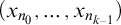
 (this initial segment we call the domain of D), which takes as input the strong index of a finite set of natural numbers
$\vec {n}=\{n_{0}<n_{1}<\dots <n_{k-1}\}$
(this initial segment we call the domain of D), which takes as input the strong index of a finite set of natural numbers
$\vec {n}=\{n_{0}<n_{1}<\dots <n_{k-1}\}$
 and outputs the c.e. index
$t(\vec {n})$
and outputs the c.e. index
$t(\vec {n})$
 for an atomic
$\mathcal {L}'$
for an atomic
$\mathcal {L}'$
 -type
${\mathrm{tp}} (\vec {n})$
-type
${\mathrm{tp}} (\vec {n})$
 in the variables
$(x_{n_{0}},\dots ,x_{n_{k-1}})$
in the variables
$(x_{n_{0}},\dots ,x_{n_{k-1}})$
 , with the compatibility condition that if
$\vec {n}\subseteq \vec {m}$
, with the compatibility condition that if
$\vec {n}\subseteq \vec {m}$
 then
${\mathrm{tp}} (\vec {n})\subseteq {\mathrm{tp}} (\vec {m})$
then
${\mathrm{tp}} (\vec {n})\subseteq {\mathrm{tp}} (\vec {m})$
 .
.
Definition 1.17. We work in the computable infinitary language, as described in [Reference Montalbán17, Chapter III].
Given a relational signature
$\mathcal {L}'$
 , we define a
$\bigvee\mathchoice{\hspace{-1.1em}}{\hspace{-0.7em}}{\hspace{-0.7em}}{\hspace{-0.6em}}\bigvee^{\mathrm {c}}_{0}$
, we define a
$\bigvee\mathchoice{\hspace{-1.1em}}{\hspace{-0.7em}}{\hspace{-0.7em}}{\hspace{-0.6em}}\bigvee^{\mathrm {c}}_{0}$
 formula as a formula of the type
$\varphi (\vec {x})\equiv P_{1}\land \dots \land P_{n}$
formula as a formula of the type
$\varphi (\vec {x})\equiv P_{1}\land \dots \land P_{n}$
 , where each
$P_{j}$
, where each
$P_{j}$
 is an atomic formula in
$\vec {x}$
is an atomic formula in
$\vec {x}$
 , per Definition 1.14. We also allow for
$P_{j}$
, per Definition 1.14. We also allow for
$P_{j}$
 to denote
$\top $
to denote
$\top $
 , the “true” predicate, and
$\bot $
, the “true” predicate, and
$\bot $
 , the “false” predicate.
We define a
$\bigvee\mathchoice{\hspace{-1.1em}}{\hspace{-0.7em}}{\hspace{-0.7em}}{\hspace{-0.6em}}\bigvee^{\mathrm {c}}_{1}$
 formula as a formula (in finitely many variables) of the type

where
$\{\varphi _{i}\}_{i<\omega }$
 is a computable sequence of
$\bigvee\mathchoice{\hspace{-1.1em}}{\hspace{-0.7em}}{\hspace{-0.7em}}{\hspace{-0.6em}}\bigvee^{\mathrm {c}}_{0}$
is a computable sequence of
$\bigvee\mathchoice{\hspace{-1.1em}}{\hspace{-0.7em}}{\hspace{-0.7em}}{\hspace{-0.6em}}\bigvee^{\mathrm {c}}_{0}$
 formulas.
Finally, we define the
$\bigvee\mathchoice{\hspace{-1.1em}}{\hspace{-0.7em}}{\hspace{-0.7em}}{\hspace{-0.6em}}\bigvee^{\mathrm {c}}_{2}$
 formulas as those formulas in finitely many variables of the type

where
$\{\psi _{i}\}_{i<\omega }$
 and
$\{\varphi _{i}\}_{i<\omega }$
and
$\{\varphi _{i}\}_{i<\omega }$
 are computable sequences of
$\bigvee\mathchoice{\hspace{-1.1em}}{\hspace{-0.7em}}{\hspace{-0.7em}}{\hspace{-0.6em}}\bigvee^{\mathrm {c}}_{1}$
are computable sequences of
$\bigvee\mathchoice{\hspace{-1.1em}}{\hspace{-0.7em}}{\hspace{-0.7em}}{\hspace{-0.6em}}\bigvee^{\mathrm {c}}_{1}$
 formulas.
One might imagine extending the definition to higher levels, by defining a
$\bigvee\mathchoice{\hspace{-1.1em}}{\hspace{-0.7em}}{\hspace{-0.7em}}{\hspace{-0.6em}}\bigvee^{\mathrm {c}}_{n+1}$
 formula as an infinite c.e. disjunction of conjunctions of
$\bigvee\mathchoice{\hspace{-1.1em}}{\hspace{-0.7em}}{\hspace{-0.7em}}{\hspace{-0.6em}}\bigvee^{\mathrm {c}}_{n}$
formula as an infinite c.e. disjunction of conjunctions of
$\bigvee\mathchoice{\hspace{-1.1em}}{\hspace{-0.7em}}{\hspace{-0.7em}}{\hspace{-0.6em}}\bigvee^{\mathrm {c}}_{n}$
 formulas and negations thereof, but these first levels will be sufficient for our purposes.
Definition 1.18 (QETP)
Let
$\mathcal {L}\subseteq \mathcal {L}'$
 be computable signatures, and let D be a structure over
$\mathcal {L}'$
be computable signatures, and let D be a structure over
$\mathcal {L}'$
 . We say that D satisfies the computable positive quantifier elimination and trash existence property, abbreviated to QETP, if the following properties hold:
-
(a) $\mathcal {L}$
is finite, closed under negation, and includes the predicate
$\neq $
, -
(b) For every quantifier-free $\mathcal {L}$
-type
$q(\vec {x},\vec {y})$
, there is a
$\bigvee\mathchoice{\hspace{-1.1em}}{\hspace{-0.7em}}{\hspace{-0.7em}}{\hspace{-0.6em}}\bigvee^{\mathrm {c}}_{1}$
$\mathcal {L}'$
-formula
$\chi _{q}(\vec {x})$
, computable from q, such that $$\begin{align*}D\vDash(\forall\vec{x})\left[\chi_{q}(\vec{x})\leftrightarrow(\exists\vec{y})\,q(\vec{x},\vec{y})\right]. \end{align*}$$
-
(c) There is a $0'$
-computable partial function, denoted by
$\tau $
, which takes as input a pair
$(q(\vec {x},y,\vec {z}),\varphi (\vec {x}))$
, where
$q(\vec {x},y,\vec {z})$
is a quantifier-free
$\mathcal {L}$
-typeFootnote
2
and
$\varphi (\vec {x})$
is a finitary
$\mathcal {L}'$
-formula, whose output is a
$\bigvee\mathchoice{\hspace{-1.1em}}{\hspace{-0.7em}}{\hspace{-0.7em}}{\hspace{-0.6em}}\bigvee^{\mathrm {c}}_{2} \mathcal {L}'$
-formula denoted
$\tau _{q\varphi }(\vec {x},y)$
that satisfies the following two properties:-
• For every tuple $(\vec {x},y,\vec {z})$
of elements in D, of
$\mathcal {L}$
-type
$q(\vec {x},y,\vec {z})$
, there is a formula
$\varphi (\vec {x})$
satisfied by
$\vec {x}$
such that
$(q,\varphi )$
is in the domain of
$\tau $
. Equivalently, if
$\vec {b}$
is a tuple of elements in D such that
$D\vDash \chi _{q}(\vec {b})$
, there is
$\varphi (\vec {x})$
such that
$(q,\varphi )$
is in the domain of
$\tau $
and
$D\vDash \varphi (\vec {b})$
. Moreover, -
• The following formula holds in D:
$$\begin{align*}D\vDash(\forall\vec{x})\left[\chi_{q}(\vec{x})\land\varphi(\vec{x})\rightarrow(\exists y)\tau_{q\varphi}(\vec{x},y)\right]. \end{align*}$$
-
-
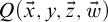
(d) Given a pair $(q(\vec {x},y,\vec {z}),\varphi (\vec {x}))$
in the domain of
$\tau $
as above, together with a quantifier-free
$\mathcal {L}$
-type
$Q(\vec {x},y,\vec {z},\vec {w})$
extending
$q(\vec {x},y,\vec {z})$
, there is a
$\bigvee\mathchoice{\hspace{-1.1em}}{\hspace{-0.7em}}{\hspace{-0.7em}}{\hspace{-0.6em}}\bigvee^{\mathrm {c}}_{1} \mathcal {L}'$
-formula
$\varepsilon \tau _{q\varphi Q}(\vec {x})$
, computable from the triple
$(q,\varphi ,Q)$
, such that $$\begin{align*}D\vDash(\forall\vec{x})\biggl[(\exists y)\left[\chi_{Q}(\vec{x},y)\land\tau_{q\varphi}(\vec{x},y)\right]\leftrightarrow\varepsilon\tau_{q\varphi Q}(\vec{x})\biggr]. \end{align*}$$The function $(q,\varphi ,Q)\mapsto \varepsilon \tau _{q\varphi Q}$
may be defined in some cases even if the pair
$(q,\varphi )$
is not in the domain of
$\tau $
. In this scenario, we do not make any requirement of
$\varepsilon \tau _{q\varphi Q}$
.
Note: As a corollary of (c), we obtain $D\vDash (\forall \vec {x})\left [\chi _{q}(\vec {x})\land \varphi (\vec {x})\rightarrow \varepsilon \tau _{q\varphi q}(\vec {x})\right ]$
for
$(q,\varphi )$
in the domain of
$\tau $
. -
(e) Finally, for all q, $\varphi $
, Q, we require $$\begin{align*}D\vDash(\forall\vec{x},y)\left[\varepsilon\tau_{q\varphi Q}(\vec{x})\land\tau_{q\varphi}(\vec{x},y)\rightarrow\chi_{Q}(\vec{x},y)\right]. \end{align*}$$
















We now state the central result of this article.
Theorem 2.6
If D is a
$0'$
 -computable c.e.-typed structure over the signature
$\mathcal {L}'\supseteq \mathcal {L}$
-computable c.e.-typed structure over the signature
$\mathcal {L}'\supseteq \mathcal {L}$
 satisfying the QETP, then the reduct
$D\mathord {\upharpoonright }\mathcal {L}$
satisfying the QETP, then the reduct
$D\mathord {\upharpoonright }\mathcal {L}$
 admits a computable copy M. There is a
$0'$
admits a computable copy M. There is a
$0'$
 -computable isomorphism between
$D\mathord {\upharpoonright }\mathcal {L}$
-computable isomorphism between
$D\mathord {\upharpoonright }\mathcal {L}$
 and M. This result is uniform in the index for D and an index for witnesses that D satisfies the QETP,Footnote
3
and relativizes uniformly.
and M. This result is uniform in the index for D and an index for witnesses that D satisfies the QETP,Footnote
3
and relativizes uniformly.
We obtain some known results as corollaries of Theorem 2.6 (see Section 3).
An extended version of this article can be found in [Reference Maia14].
2 A general jump inversion theorem
2.1 Preliminary observations
Before the main proof of this article, we make some observations that will be necessary regarding the new types of formulas we introduced in Definition 1.17 and regarding the definition of the QETP (Definition 1.18).
Remark 2.1. The main property of the
$\bigvee\mathchoice{\hspace{-1.1em}}{\hspace{-0.7em}}{\hspace{-0.7em}}{\hspace{-0.6em}}\bigvee^{\mathrm {c}}_{1}$
 formulas is: Given a c.e. index for the atomic
$\mathcal {L}'$
formulas is: Given a c.e. index for the atomic
$\mathcal {L}'$
 -type of a tuple of elements
$\vec {b}$
-type of a tuple of elements
$\vec {b}$
 in some structure, and a
$\bigvee\mathchoice{\hspace{-1.1em}}{\hspace{-0.7em}}{\hspace{-0.7em}}{\hspace{-0.6em}}\bigvee^{\mathrm {c}}_{1}$
in some structure, and a
$\bigvee\mathchoice{\hspace{-1.1em}}{\hspace{-0.7em}}{\hspace{-0.7em}}{\hspace{-0.6em}}\bigvee^{\mathrm {c}}_{1}$
 formula
$\varphi (\vec {x})$
formula
$\varphi (\vec {x})$
 satisfied by
$\vec {b}$
satisfied by
$\vec {b}$
 , we can computably confirm in finite time that the tuple
$\vec {b}$
, we can computably confirm in finite time that the tuple
$\vec {b}$
 satisfies the formula
$\varphi $
satisfies the formula
$\varphi $
 .
.
Remark 2.2. The main property of the
$\bigvee\mathchoice{\hspace{-1.1em}}{\hspace{-0.7em}}{\hspace{-0.7em}}{\hspace{-0.6em}}\bigvee^{\mathrm {c}}_{2}$
 formulas is: Given a tuple of elements
$\vec {b}$
formulas is: Given a tuple of elements
$\vec {b}$
 of a structure and a c.e. index for the atomic type of
$\vec {b}$
of a structure and a c.e. index for the atomic type of
$\vec {b}$
 , it is
$0'$
, it is
$0'$
 -c.e. to determine whether a
$\bigvee\mathchoice{\hspace{-1.1em}}{\hspace{-0.7em}}{\hspace{-0.7em}}{\hspace{-0.6em}}\bigvee^{\mathrm {c}}_{2}$
-c.e. to determine whether a
$\bigvee\mathchoice{\hspace{-1.1em}}{\hspace{-0.7em}}{\hspace{-0.7em}}{\hspace{-0.6em}}\bigvee^{\mathrm {c}}_{2}$
 formula holds of
$\vec {b}$
formula holds of
$\vec {b}$
 .
.
To elaborate: If
$\varphi (\vec {x})\equiv \bigvee\mathchoice{\hspace{-1.1em}}{\hspace{-0.7em}}{\hspace{-0.7em}}{\hspace{-0.6em}}\bigvee_{i}\left (\psi _{i}(\vec {x})\land \neg \varphi _{i}(\vec {x})\right )$
 is a
$\bigvee\mathchoice{\hspace{-1.1em}}{\hspace{-0.7em}}{\hspace{-0.7em}}{\hspace{-0.6em}}\bigvee^{\mathrm {c}}_{2}$
is a
$\bigvee\mathchoice{\hspace{-1.1em}}{\hspace{-0.7em}}{\hspace{-0.7em}}{\hspace{-0.6em}}\bigvee^{\mathrm {c}}_{2}$
 formula, and
$\vec {b}$
formula, and
$\vec {b}$
 is a tuple of elements of a structure for which we have a c.e. index for the atomic type of
$\vec {b}$
is a tuple of elements of a structure for which we have a c.e. index for the atomic type of
$\vec {b}$
 , we can computably create a sequence of guesses for whether
$\varphi (\vec {b})$
, we can computably create a sequence of guesses for whether
$\varphi (\vec {b})$
 holds: Guess ‘no’ until we find i for which
$\psi _{i}(\vec {b})$
holds: Guess ‘no’ until we find i for which
$\psi _{i}(\vec {b})$
 holds. Then guess ‘yes’ until we find that
$\varphi _{i}(\vec {b})$
holds. Then guess ‘yes’ until we find that
$\varphi _{i}(\vec {b})$
 holds. Again guess ‘no’ until we find a new j for which
$\psi _{j}(\vec {b})$
holds. Again guess ‘no’ until we find a new j for which
$\psi _{j}(\vec {b})$
 holds, then ‘yes’ until we find that
$\varphi _{j}(\vec {b})$
holds, then ‘yes’ until we find that
$\varphi _{j}(\vec {b})$
 holds, and so on. This sequence of guesses will have the following behavior:
-
• if $\varphi (\vec {b})$
holds, we will guess ‘yes’ all but finitely many times, and -
• if $\varphi (\vec {b})$
does not hold, we will guess ‘no’ infinitely many times.


Remark 2.3. Bazhenov et al. introduced in [Reference Bazhenov, Fokina, Rossegger, Soskova and Vatev2] two hierarchies of infinitary formulas, which they named
$\Sigma _{\alpha }^{p}$
 and
$\Pi _{\alpha }^{p}$
and
$\Pi _{\alpha }^{p}$
 for
$\alpha <\omega _{1}$
for
$\alpha <\omega _{1}$
 , which are defined with positivity of predicates in mind.Footnote
4
These are closely related to our work: Our
$\bigvee\mathchoice{\hspace{-1.1em}}{\hspace{-0.7em}}{\hspace{-0.7em}}{\hspace{-0.6em}}\bigvee^{\mathrm {c}}_{n}$
, which are defined with positivity of predicates in mind.Footnote
4
These are closely related to our work: Our
$\bigvee\mathchoice{\hspace{-1.1em}}{\hspace{-0.7em}}{\hspace{-0.7em}}{\hspace{-0.6em}}\bigvee^{\mathrm {c}}_{n}$
 formulas coincide exactly with the set of quantifier-free
$\Sigma _{n}^{p}$
formulas coincide exactly with the set of quantifier-free
$\Sigma _{n}^{p}$
 formulas.
Remark 2.4. We will work with Item (c) of the QETP in the following manner: We envision a computable process that enumerates triples
$(q,\varphi ,\tau )$
 , and sometimes deletes them, in such a manner that, if
$\tau _{q\varphi }$
, and sometimes deletes them, in such a manner that, if
$\tau _{q\varphi }$
 is well-defined, the triple
$(q,\varphi ,\tau _{q\varphi })$
is well-defined, the triple
$(q,\varphi ,\tau _{q\varphi })$
 will eventually be enumerated and never removed, and every triple that is not of the form
$(q,\varphi ,\tau _{q\varphi })$
will eventually be enumerated and never removed, and every triple that is not of the form
$(q,\varphi ,\tau _{q\varphi })$
 for
$(q,\varphi )$
for
$(q,\varphi )$
 in the domain of
$\tau $
in the domain of
$\tau $
 will eventually be removed.
Remark 2.5. We make an additional technical assumption on the formulas
$\chi _{q}$
 with no loss of generality. Let
$q(\vec {x},\vec {y},\vec {z})$
with no loss of generality. Let
$q(\vec {x},\vec {y},\vec {z})$
 be a quantifier-free
$\mathcal {L}$
be a quantifier-free
$\mathcal {L}$
 formula. We can assign a
$\chi $
formula. We can assign a
$\chi $
 -formula to q in (at least) two different ways: By grouping the variables as
$(\vec {x},[\vec {y},\vec {z}])$
-formula to q in (at least) two different ways: By grouping the variables as
$(\vec {x},[\vec {y},\vec {z}])$
 , or by grouping them as
$([\vec {x},\vec {y}],\vec {z})$
, or by grouping them as
$([\vec {x},\vec {y}],\vec {z})$
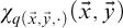
 . This leads to two different formulas, which, when necessary to distinguish, we notate, respectively, as
$\chi _{q(\vec {x},\cdot ,\cdot )}(\vec {x})$
. This leads to two different formulas, which, when necessary to distinguish, we notate, respectively, as
$\chi _{q(\vec {x},\cdot ,\cdot )}(\vec {x})$
 and
$\chi _{q(\vec {x},\vec {y},\cdot )}(\vec {x},\vec {y})$
and
$\chi _{q(\vec {x},\vec {y},\cdot )}(\vec {x},\vec {y})$
 . Now, we assume without loss of generality that, in such a scenario,
$\chi _{q(\vec {x},\vec {y},\cdot )}(\vec {x},\vec {y})$
. Now, we assume without loss of generality that, in such a scenario,
$\chi _{q(\vec {x},\vec {y},\cdot )}(\vec {x},\vec {y})$
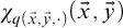 contains
$\chi _{q(\vec {x},\cdot ,\cdot )}(\vec {x})$
contains
$\chi _{q(\vec {x},\cdot ,\cdot )}(\vec {x})$
 as a subformula.
The reason why we can make such an assumption is that, given a quantifier-free
$\mathcal {L}$
 -formula
$q(\vec {x},\vec {y})$
-formula
$q(\vec {x},\vec {y})$
 , we may redefine
$\bar {\chi }_{q}(\vec {x})$
, we may redefine
$\bar {\chi }_{q}(\vec {x})$
 as
as

where the conjunction ranges over all decompositions of the tuple
$\vec {x}$
 into two tuples of variables (not necessarily in order).
2.2 Main result
Theorem 2.6. If D is a
$0'$
 -computable c.e.-typed structure over the signature
$\mathcal {L}'\supseteq \mathcal {L}$
-computable c.e.-typed structure over the signature
$\mathcal {L}'\supseteq \mathcal {L}$
 satisfying the QETP, then the reduct
$D\mathord {\upharpoonright }\mathcal {L}$
satisfying the QETP, then the reduct
$D\mathord {\upharpoonright }\mathcal {L}$
 admits a computable copy M. There is a
$0'$
admits a computable copy M. There is a
$0'$
 -computable isomorphism between
$D\mathord {\upharpoonright }\mathcal {L}$
-computable isomorphism between
$D\mathord {\upharpoonright }\mathcal {L}$
 and M. This result is uniform in the index for D and an index for witnesses that D satisfies the QETP,Footnote
5
and relativizes uniformly.
and M. This result is uniform in the index for D and an index for witnesses that D satisfies the QETP,Footnote
5
and relativizes uniformly.
Proof. We build a computable copy of
$D\mathord {\upharpoonright }\mathcal {L}$
 via a finite injury argument. First, some background assumptions:
-
• We see the structure D as being given by a computable process, which outputs elements and c.e. indices for the atomic $\mathcal {L}'$
-type of the elements output until now, and sometimes erases previously constructed elements. We will be executing this construction in parallel in the background of ours. -
• An element of D which is added in this manner and never removed will be referred to as a real element of D.
-
• We will build the $\mathcal {L}$
-structure
$M\cong D\mathord {\upharpoonright }\mathcal {L}$
via a computable process that outputs a sequence of elements, and with each element, the quantifier-free
$\mathcal {L}$
-type of the elements output until now. -
• We well-order the elements of M and the elements of D by time of addition. This includes “fake” elements of D. When we refer to “the first element of M (or D) that satisfies such-and-such property,” we mean the one that was added earliest.
-
• We will imagine an assortment of agents, referred to as “agent i” for $i=0,1,2,\dots $
, each of which will be responsible for one step in a back-and-forth construction of an isomorphism between D and the structure M that we are constructing. Roughly speaking, agent i will be responsible for satisfying the requirement: The i-th real element of D is matched to an element of M, and the i-th element of M is matched to an element of D, and the matchings created by agents
$0$
to i form an isomorphism of finite
$\mathcal {L}$
-structures. We describe requirement i in more detail below, by describing how it may be injured, after we have introduced some further notation about the construction. -
• We assume that only one agent is active at each time. When agent i is done with its task, it will activate agent $i+1$
. When an injury occurs, we divert execution back to a prior agent, say agent j, and delete the state of all agents past agent j. -
• The internal state of this construction, that is, the information we will be keeping track of, consists of the following data (plus whatever auxiliary information is necessary to keep track of the agent mechanism):
-
– The current status of the structures M and D.
-
– One-to-one matchings between some elements of M and some elements of D, the latter of which may or may not be real.
-
– To some elements m of M, we match a triple of formulas $(q(\vec {x},y,\vec {z}),\varphi (\vec {x}), \tau (\vec {x},y))$
that have been output by the process from Remark 2.4, together with a decomposition of the elements of M at the time that this matching was created into tuples
$\vec {x}$
,
$y=m$
, and
$\vec {z}$
. -
– To each matching of the previous two kinds, we keep track of which agent created it and when.
-
-
• The internal state of this construction may be modified via the following operations:
-
– We may add a new element to M, in which case we immediately match it to an element of D.
-
– We may match a triple of formulas $(q,\varphi ,\tau )$
to an unmatched element
$y\in M$
, together with the decomposition
$M_{\mathrm {current}}=(\vec {x},y,\vec {z})$
, where
$\vec {x}$
denotes the elements of M that have a match in D at this moment. -
– We may create a matching between an element of M and an element of D, if the element of M has a triple $(q,\varphi ,\tau )$
assigned. -
– In the event of injury, we may remove matches of the three kinds above.
-
-
• We say that requirement i is injured if any of the following three things happen:
-
– An element of D which was matched by agent i to an element of M is deleted.
-
– There is an element of M, to whom agent i matched a triple of formulas $(q,\varphi ,\tau )$
, for which the triple of formulas has been deleted from the enumeration of the process of Remark 2.4. -
– There is an element of M, to whom agent i matched a triple of formulas $(q,\varphi ,\tau )$
, and a matched element
$d\in D$
, such that our guess about whether
$\tau $
holds of this element has changed to ‘no’.
In any of these cases, all matches created after the “faulty match” will be deleted.
-







Now we list some conditions to be maintained, barring injury. Together with each assumption, we point out the operations that we need to be careful in exercising—the remaining operations will always preserve the given assumption. Moreover, the assumptions will not be broken with the passage of time unless injury happens, in which case the injury-handling part of the algorithm will rectify any issues.
-
Assumption (A) If $M=(\vec {x},\vec {y})$
, where
$\vec {x}$
denotes the elements of M that currently admit matches in D,
$\vec {b}$
denotes these matches, and
$q(\vec {x},\vec {y})$
is the type of the elements of M, we demand that
$D\vDash \chi _{q}(\vec {b})$
.We need to be careful to ensure that this is true when we add new elements to M, and when we create matches between elements of M and elements of D. We would also need to be careful in the event that matches are deleted, but this is where Remark 2.5 becomes relevant, as it ensures that this is not a concern.
-
Assumption (B) If $y\in M$
is matched with a triple of formulas
$(q,\varphi ,\tau )$
and decomposition
$(\vec {x},y,\vec {z})\subseteq M$
, we demand that
$M\vDash q(\vec {x},y,\vec {z})$
and that all elements of
$\vec {x}$
admit matches
$\vec {b}$
in D, which satisfy
$D\vDash \varphi (\vec {b})$
.We need to be careful to ensure that this is true when we assign a triple to an element. We don’t need to be careful when removing matches or elements of D, because our injury process will, in that case, unmatch the formulas assigned to y.
-
Assumption (C) At most one unmatched element m of M will have an assigned triple at any given time, and in this event, the variables $\vec {x}$
correspond to the elements of M currently matched to elements of D, and the next action to be taken will be to match m to an element of D. -
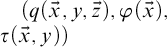
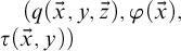
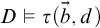
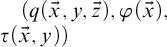
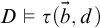
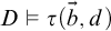
Assumption (D) If y is an element of M with assigned triple $(q(\vec {x},y,\vec {z}),\varphi (\vec {x}), \tau (\vec {x},y))$
and y admits a match d in D, if
$\vec {b}$
is the tuple of elements matched with
$\vec {x}$
, it must be the case that
$D\vDash \tau (\vec {b},d)$
at the current approximation (in the sense of Remark 2.2).We need to be careful to ensure that this is true when we create a match between an element of M with an assigned triple $(q,\varphi ,\tau )$
and an element of D. We also need to be careful if the current approximation (in the sense of Remark 2.2) ever changes, which is why ‘the approximation of the value of
$\tau (\vec {b},d)$
changes’ is a cause of injury. -
Assumption (E) If m is an element with assigned formulas $(q(\vec {x},y,\vec {z}),\varphi (\vec {x}), \tau (\vec {x},y))$
, with
$\vec {b}$
denoting the matches of the
$\vec {x}$
, and at this stage M is decomposed as
$M=(\vec {x},y,\vec {z},\vec {w})$
with quantifier-free
$\mathcal {L}$
-type
$Q(\vec {x},y,\vec {z},\vec {w})$
, it must be the case that, if the
$\vec {b}$
are real elements of D, we have
$D\vDash \varepsilon \tau _{q\varphi Q}(\vec {b})$
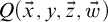
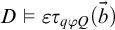
.We need to be careful to ensure that this is true when new elements are added to M, and when we assign triples $(q,\varphi ,\tau )$
to elements of M.














The process starts with the initialization of agent
$0$
 .
.
Now we describe the algorithm that will be followed by agent i. When agent i is initialized:
-
Step I. Find the first element of M, if any, that does not have a match in D. If there is none, skip to Step V. If there is one, call it m.
-
Step II. If m has an assigned triple of formulas $(q,\varphi ,\tau )$
, skip to Step IV.Footnote
6
-
Step III. If m does not have an assigned triple: Let $(\vec {x},y,\vec {z})$
be the current elements of M, with
$\vec {x}$
corresponding to the elements that currently have a match in D—call their matches
$\vec {b}$
—, y corresponding to m, and
$\vec {z}$
corresponding to the remaining elements. Look through the triples
$(q,\varphi ,\tau )$
enumerated as per Remark 2.4 until you find such a triple that satisfies
$M\vDash q(\vec {x},y,\vec {z})$
and
$D\vDash \varphi (\vec {b})$
. If all elements of
$\vec {b}$
are real, such a triple will be found in finite time by Assumption (A) in conjunction with Item (c) of the QETP. If not all are real, injury will happen. Once such a triple is found, we assign to m the triple
$(q,\varphi ,\tau )$
with the decomposition
$(\vec {x},y,\vec {z})$
above.We need to make sure that Assumption (B) and Assumption (E) are preserved.
-
• Assumption (B)—By design.
-
• Assumption (E)—We need to guarantee that, if the $\vec {b}$
are all real, we have
$D\vDash \varepsilon \tau _{q\varphi q}(\vec {b})$
. This is a consequence of the note at the end of Item (d) of the QETP.
-
-
Step IV. Let $(q,\varphi ,\tau )$
be the formula assigned to m. The formula
$q(\vec {x},y,\vec {z})$
will not, in general, be the quantifier-free
$\mathcal {L}$
-type of the current elements of M, but it is definitely the quantifier-free
$\mathcal {L}$
-type of some subset of elements of M. By Assumption (C), the elements corresponding to
$\vec {x}$
are exactly the ones that currently admit matches in D. Let
$\vec {b}$
denote their matches.We let $Q(\vec {x},y,\vec {z},\vec {w})$
denote the quantifier-free type of the current elements of M, where
$\vec {x}$
, y, and
$\vec {z}$
are the same as above.Look through the elements of D until you find an element d satisfying $D\vDash \tau (\vec {b},d)$
to current approximation (in the sense of Remark 2.2).Technical note: This search must be done in some systematic way so that, if all $\vec {b}$
are real, we eventually find a real element d satisfying this formula in such a way that the approximation stays fixed. An example of such a systematic way: Let’s say we give the n-th element added to D, say
$d_{n}$
, a penalty of n stages in the time it takes to compute whether
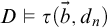
$D\vDash \tau (\vec {b},d_{n})$
, and select the d such that
$D\vDash \tau (\vec {b},d)$
is verified (and not disproven until now) in the least amount of stages. This will be important when proving finite injury.We claim that, unless an injury occurs, this search will eventually terminate. By this we mean: Assume that all $\vec {b}$
are real, and that the triple
$(q,\varphi ,\tau )$
will never be removed from the enumeration from Remark 2.4. Then, by Assumption (A) it must be the case that
$D\vDash \chi _{Q}(\vec {b})$
and by Assumption (E) it must be the case that
$D\vDash \varepsilon \tau _{q\varphi Q}(\vec {b})$
. Thus, by Item (d) of the QETP, it must be the case that
$D\vDash (\exists y)\tau _{q}(\vec {b},y)$
, and any witness to this statement will serve as the d above.Once such a d is found, we match m to d.
We need to make sure that Assumption (A) and Assumption (D) hold.
-
• Assumption (A)—If d is real, this is direct by Item (e) of the QETP.
-
• Assumption (D)—By construction.
-
-
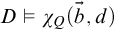
Step V. Next, find the first element of D—call it d—that does not have a match in M. If there is no such element as of right now, proceed to Step VI.
Let $q(\vec {x},\vec {y})$
be the quantifier-free
$\mathcal {L}$
-type of the current elements of M, with
$\vec {x}$
denoting the elements that currently have matches in D, and let
$\vec {b}$
denote their matches. Let
$r(\vec {x},z)$
be the quantifier-free
$\mathcal {L}$
-type of the tuple
$(\vec {b},d)$
.Footnote
7
In parallel, look through the quantifier-free
$\mathcal {L}$
existential types
$Q(\vec {x},z,\vec {y})$
until you find such a Q extending
$q(\vec {x},\vec {y})\land r(\vec {x},z)$
such that:-
• $D\vDash \chi _{Q(\vec {x},z,\cdot )}(\vec {b},d)$
, and -
• for every m with an assigned triple $(q_{0}(\vec {x}_{0},y_{0},\vec {z}_{0}),\varphi (\vec {x}_{0}),\tau (\vec {x}_{0},y_{0}))$
, if
$\vec {b}_{0}$
are the elements of M corresponding to
$\vec {x}_{0}$
,
$D\vDash \varepsilon \tau _{q_{0}\varphi Q}(\vec {b}_{0})$
.
We argue that either such a Q is found in finite time or otherwise an injury will occur. Indeed, suppose that both d and the elements of $\vec {b}$
are all real, and that every matched triple
$(q_{0},\varphi ,\tau )$
will never be injured. Now, since we assume
$D\vDash \chi _{q}(\vec {b})$
, there must be a tuple of real elements
$\vec {c}$
in D such that
$D\vDash q(\vec {b},\vec {c})$
. Now, we claim that the type Q of the tuple
$(\vec {b},d,\vec {c})$
satisfies the desired requisites:-
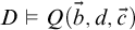
• Since $D\vDash Q(\vec {b},d,\vec {c})$
, we must have
$D\vDash (\exists \vec {y})Q(\vec {b},d,\vec {y})$
and hence
$D\vDash \chi _{Q}(\vec {b},d)$
. -
• If m has the triple $(q_{0},\varphi ,\tau )$
assigned, with decomposition
$(\vec {x}_{0},y_{0},\vec {z}_{0})\subseteq M$
, with
$\vec {b}_{0}$
being the elements of D corresponding to
$\vec {x}_{0}$
and
$d_{0}$
being the element corresponding to m, we have
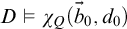
$D\vDash \chi _{Q}(\vec {b}_{0},d_{0})$
as a consequence of
$D\vDash Q(\vec {b},d,\vec {c})$
, and moreover
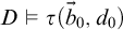
$D\vDash \tau (\vec {b}_{0},d_{0})$
by Assumption (D), hence
$D\vDash (\exists y)\left [\chi _{Q}(\vec {b}_{0},y)\land \tau _{q\varphi }(\vec {b}_{0},y)\right ]$
, and thus
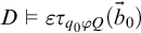
$D\vDash \varepsilon \tau _{q_{0}\varphi Q}(\vec {b}_{0})$
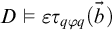
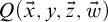
by Item (d) of the QETP.
Once such a $Q(\vec {x},z,\vec {y})$
is found, one of two things occurs. Either it includes
$z=y_{j}$
for some value of j, in which case we match d to the element corresponding to
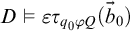
$y_{j}$
, or it includes the information that all its variables represent distinct elements, in which case we add a new element to M, whose relations to the previous elements are those dictated by Q, and match it to d.We need to make sure that Assumption (A) and Assumption (E) hold.
-
• Assumption (A)—By construction, since we ensured $D\vDash \chi _{Q}(\vec {b},d)$
. -
• Assumption (E)—By construction.
-
-
Step VI. Once all the above steps are done, agent i will pause its execution, and initialize agent $i+1$
.
























We now describe the process of injury. There are three means of injury:
-
• Suppose that an element of D is seen to be removed. If this element does not have a match in M, no action is taken. On the other hand, suppose that this element d is matched to an element m in M. In that event, suppose that agent i is the one that made this match, and halt the execution of all agents with index greater than i, erasing matches and assigned formulas created past the moment that m and d were matched. If the match between d and m was created by Step I, restart the execution of agent i. If the match between d and m was created by Step V, initialize agent $i+1$
(and do not restart agent i). -
• Suppose that an element $m\in M$
has an assigned triple
$(q,\varphi ,\tau )$
, which is seen to be deleted from the enumeration described in Remark 2.4 at a given stage. Suppose agent i is the one who has assigned this formula. Then, we halt the execution of all agents with index greater than i, and erase all matches and assigned formulas created past the moment that this formula was assigned to m. Then, execute agent i starting in Step III. -
• Suppose that an element $m\in M$
has an assigned triple
$(q(\vec {x},y,\vec {z}),\varphi (\vec {x}),\tau (\vec {x},y))$
and a matched element d. Suppose agent i is the one who has created these matches. Suppose that the elements
$\vec {x}$
are matched to the tuple
$\vec {b}$
, and suppose that the current approximation of
$D\vDash \tau (\vec {b},d)$
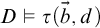
(in the sense of Remark 2.2) has changed to ‘no’. Then, we halt the execution of all agents with index greater than i, erase all matches and assigned formulas created past this point (including the match between m and d, but we retain the assigned triple
$(q,\varphi ,\tau )$
), and execute agent i starting in Step IV.






This concludes the construction. It remains to show that the resulting structure M is isomorphic to
$D\mathord {\upharpoonright }\mathcal {L}$
 , and this is done via a finite injury argument. We show that each requirement will be injured finitely many times. This will show that every element in D is eventually matched to an element of M (the i-th element of D (counting both real and fake elements) will be matched by, at worst, the i-th agent past the moment when this element is added to D), and that every element of M is eventually matched to an element of D (given an orphan element of M, inductively consider the first agent activated after all previous elements of M have been matched), and since these matches all preserve the predicates in
$\mathcal {L}$
, and this is done via a finite injury argument. We show that each requirement will be injured finitely many times. This will show that every element in D is eventually matched to an element of M (the i-th element of D (counting both real and fake elements) will be matched by, at worst, the i-th agent past the moment when this element is added to D), and that every element of M is eventually matched to an element of D (given an orphan element of M, inductively consider the first agent activated after all previous elements of M have been matched), and since these matches all preserve the predicates in
$\mathcal {L}$
 , the resulting map will be an isomorphism.
Suppose, for the sake of induction, that all requirements prior to i are injured finitely many times. We show that requirement i itself also suffers finite injury. We do this individually for each of the matches potentially created by agent i:
-
• First, we show that the matching created by the first orphan element of m at this moment, if there is any, is injured finitely many times. Indeed, per the notation of Remark 2.4 and using Item (c) of the QETP, eventually a triple $(q,\varphi ,\tau )$
will be enumerated and never removed, such that the relevant elements of D satisfy
$\chi _{q}\land \varphi $
. Past this point, after all previously-added false triples have been removed, this triple (or another) will be permanently assigned to m. Afterward, we know (see the technical note in Step IV) that after enough steps we match m with a real element d of D that satisfies
$\tau (\vec {b},d)$
at the current approximation, which will then stay fixed. This match will never cause injury. -
• Now, assuming that we’ve reached a time where the matching discussed in the previous bullet point or created by previous agents will never be removed, suppose that there is an unmatched element in D for agent i to match with an element of M. If this element is real, there is no injury. If the element is not real, then it is eventually erased. Then execution will move to agent $i+1$
, and requirement i is never injured.


This concludes the proof.
3 Previously known applications
In this section, we list some known results that can be obtained using Theorem 2.6. We give the proof just for the most interesting one.
3.1 Elementary results
Theorem 3.1 [Reference Montalbán16, Lemma VII.26]
Suppose that L is a linear order for which every element admits a successor and predecessor, and suppose that the structure
$(L,<,S)$
 admits a
$0'$
admits a
$0'$
 -computable copy, where
$S(x,y)$
-computable copy, where
$S(x,y)$
 is the successor relation. Then, the structure
$(L,<)$
is the successor relation. Then, the structure
$(L,<)$
 admits a computable copy.
Proof. Omitted. See [Reference Maia14].
Proposition 3.2 (Folklore, [Reference Downey and Melnikov4, Theorem 9.1.4])
Let
$(E,\simeq )$
 be an equivalence relation with infinitely many infinite equivalence classes, and assume that the structure
$(E,\simeq ,\{P_{\geq n}\}_{n\in \mathbb {N}})$
be an equivalence relation with infinitely many infinite equivalence classes, and assume that the structure
$(E,\simeq ,\{P_{\geq n}\}_{n\in \mathbb {N}})$
 admits a
$0'$
admits a
$0'$
 -computable copy, where
$P_{\geq n}(x)$
-computable copy, where
$P_{\geq n}(x)$
 is the predicate “the equivalence class of x has size at least n.”Footnote
8
Then,
$(E,\simeq )$
is the predicate “the equivalence class of x has size at least n.”Footnote
8
Then,
$(E,\simeq )$
 admits a computable copy.
Proof. Omitted. See [Reference Maia14].
Definition 3.3 (Khisamiev, [Reference Downey and Melnikov4, Definition 9.1.3])
A set
$X\subseteq \mathbb {N}$
 is said to be limitwise monotonic if there is a total computable function
$f\colon \mathbb {N}\times \mathbb {N}\to \mathbb {N}$
is said to be limitwise monotonic if there is a total computable function
$f\colon \mathbb {N}\times \mathbb {N}\to \mathbb {N}$
 such that, for every
$x\in \mathbb {N}$
such that, for every
$x\in \mathbb {N}$
 , the sequence
$\{f(x,y)\}_{y\in \mathbb {N}}$
, the sequence
$\{f(x,y)\}_{y\in \mathbb {N}}$
 is weakly increasing (i.e., nondecreasing) and bounded (and therefore convergent), and X is the image of the pointwise limit function
$g(x)=\lim _{y}f(x,y)$
is weakly increasing (i.e., nondecreasing) and bounded (and therefore convergent), and X is the image of the pointwise limit function
$g(x)=\lim _{y}f(x,y)$
 .
.
Definition 3.4 [Reference Downey and Melnikov4, Definition 9.1.1]
Let
$(E,\simeq )$
 be an equivalence relation. The characteristic set of E is the set

Proposition 3.5 (Folklore, [Reference Downey and Melnikov4, Theorem 9.1.4])
Let
$(E,\simeq )$
 be an equivalence relation with finitely many infinite equivalence classes, and assume that the structure
$(E,\simeq ,\{P_{\geq n}\}_{n\in \mathbb {N}})$
be an equivalence relation with finitely many infinite equivalence classes, and assume that the structure
$(E,\simeq ,\{P_{\geq n}\}_{n\in \mathbb {N}})$
 admits a
$0'$
admits a
$0'$
 -computable copy, where
$P_{\geq n}(x)$
-computable copy, where
$P_{\geq n}(x)$
 is the predicate “the equivalence class of x has size at least n.” Assume moreover that the characteristic set of E is limitwise monotonic. Then,
$(E,\simeq )$
is the predicate “the equivalence class of x has size at least n.” Assume moreover that the characteristic set of E is limitwise monotonic. Then,
$(E,\simeq )$
 admits a computable copy.
Proof. Omitted. See [Reference Maia14].
Proposition 3.6 [Reference Calvert, Frolov, Harizanov, Knight, McCoy, Soskova and Vatev3, Proposition 3.8]
Let T be an infinite subtree of
$\omega ^{<\omega }$
 such that every node of T that is not a leaf has infinitely many successors, of which finitely many are leaves. For the signature, we use the successor relation
$S(x,y)$
such that every node of T that is not a leaf has infinitely many successors, of which finitely many are leaves. For the signature, we use the successor relation
$S(x,y)$
 and a unary relation
$R_{0}(x)$
and a unary relation
$R_{0}(x)$
 for the root. The other important predicate for a structural jump is
${\mathrm{leaf}} (x)$
for the root. The other important predicate for a structural jump is
${\mathrm{leaf}} (x)$
 (x is a leaf).
If the structure
$(T,{\mathrm{leaf}} ,S,R_{0})$
 admits a
$0'$
admits a
$0'$
 -computable copy, then the structure
$(T,S,R_{0})$
-computable copy, then the structure
$(T,S,R_{0})$
 admits a computable copy.
Proof. Omitted. See [Reference Maia14].
3.2 Khisamiev’s theorem
The following theorem is in the literature, see, e.g., Chapter 5 of [Reference Downey and Melnikov4].
In the following, we interpret a c.e. presentation of a group as being a description of the group as a list of generators and relations, such that there is a computer program that enumerates the list of generators and relations. In the present case, this is equivalent to the more general notion of c.e. presentation of a structure in computability theory.
Theorem 3.7 (Khisamiev)
Every c.e. presented torsion-free abelian group is isomorphic to a computable group. Furthermore, if the group is nontrivial, then this computable copy can be built uniformly in the index of the c.e. presentation.
Proof. Given a c.e. presentation of a group G, we first build a
$0'$
 -computable c.e.-typed copy of G over an appropriate signature
$\mathcal {L}'$
-computable c.e.-typed copy of G over an appropriate signature
$\mathcal {L}'$
 , and we will then show that any nontrivial torsion-free abelian group has the QETP (uniformly) over
$\mathcal {L}\subseteq \mathcal {L}'$
, and we will then show that any nontrivial torsion-free abelian group has the QETP (uniformly) over
$\mathcal {L}\subseteq \mathcal {L}'$
 , where
$\mathcal {L}$
, where
$\mathcal {L}$
 is the signature containing only the ternary predicate
$S(x,y,z)\equiv {\text{"}{x+y=z}\text{"}}$
is the signature containing only the ternary predicate
$S(x,y,z)\equiv {\text{"}{x+y=z}\text{"}}$
 (and its negation, and equality and its negation).
The signature
$\mathcal {L}'$
 contains
$\mathcal {L}$
contains
$\mathcal {L}$
 plus:
plus:
-
• The countably many predicates $Q_{n,\vec {c}}(\vec {x})$
, parametrized over
$n\in \mathbb {N}$
and finite tuples
$c_{1},\dots ,c_{k}\in \mathbb {Z}$
: $$\begin{align*}Q_{n,\vec{c}}(\vec{x})\equiv\text{"}{n\mid c_{1}x_{1}+\dots+c_{k}x_{k}}.\text{"} \end{align*}$$
Note that we allow n to equal zero, in which case (since $0\mid y$
iff
$y=0$
)
$Q_{0,\vec {c}}(\vec {x})$
corresponds to the predicate
$\vec {c}\cdot \vec {x}=0$
. -
• The countably many predicates $\neg Q_{0,\vec {c}}(\vec {x})$
, parametrized over finite tuples
$c_{1},\dots ,c_{k}\in \mathbb {Z}$
: $$\begin{align*}\neg Q_{0,\vec{c}}(\vec{x})\equiv{\text{"}{c_{1}x_{1}+\dots+c_{k}x_{k}\neq0}.\text{"}} \end{align*}$$
-
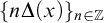
• Countably many predicates $\{n\Delta (x)\}_{n\in \mathbb {Z}}$
, whose meaning is as follows: We will carefully pick a single designated nonzero element of G, which we refer to as
$\delta $
, and
$n\Delta (x)$
should be interpreted as “
$x=n\delta $
.”









We need some linear algebra of
$\mathbb {Z}$
 -modules to show that, from a c.e. presentation of G, we can uniformly obtain a
$0'$
-modules to show that, from a c.e. presentation of G, we can uniformly obtain a
$0'$
 -computable c.e.-typed copy of G. Then, we will explain how we choose the element of G that will be tagged with
$\Delta $
-computable c.e.-typed copy of G. Then, we will explain how we choose the element of G that will be tagged with
$\Delta $
 . To obtain the
$0'$
. To obtain the
$0'$
 -computable c.e.-typed copy of G, here is the basic idea: Consider the computable process that outputs all possible linear combinations of generators. We want to, with each new linear combination of generators, say d, first check whether it is equal to any of the combinations previously produced (this is an easy check with
$0'$
-computable c.e.-typed copy of G, here is the basic idea: Consider the computable process that outputs all possible linear combinations of generators. We want to, with each new linear combination of generators, say d, first check whether it is equal to any of the combinations previously produced (this is an easy check with
$0'$
 ), and if it is not, we want to output a c.e. index for its type relative to the elements previously output. This is easy for the positive predicates—to check if, for example,
$5\mid 4d+6c$
), and if it is not, we want to output a c.e. index for its type relative to the elements previously output. This is easy for the positive predicates—to check if, for example,
$5\mid 4d+6c$
 (where c is a previously output combination of generators), it suffices to check if there is a further combination of generators u that satisfies the relation
$5u-4d-6c=0$
(where c is a previously output combination of generators), it suffices to check if there is a further combination of generators u that satisfies the relation
$5u-4d-6c=0$
 . This is a c.e. check. The difficulty lies in the negative predicates, of which
$\neg Q_{0,\vec {c}}(\vec {x})$
. This is a c.e. check. The difficulty lies in the negative predicates, of which
$\neg Q_{0,\vec {c}}(\vec {x})$
 is the general case. In other words, we need to encode into a single c.e. index the full information about what linear combinations of elements-output-so-far equal zero.
Here is a fact from commutative algebra, whose proof can be found in any standard book that covers modules over principal ideal domains (e.g., [Reference Dummit and Foote5]):
-
Fact A: Any submodule M of $\mathbb {Z}^{k}$
admits a finite basis.

Here is the effective version of this fact that we will use:
-
Fact B: Given a c.e. index for a submodule M of $\mathbb {Z}^{k}$
, we may
$0'$
-effectively find a basis of M.


Proof idea: Consider the k-width and possibly-infinite-height matrix whose rows are the elements of M. Use
$0'$
 to find the GCD of the elements of the first column, call it d. If
$d=0$
to find the GCD of the elements of the first column, call it d. If
$d=0$
 (i.e., all elements of the first column are zero), skip to the next step. If
$d\neq 0$
(i.e., all elements of the first column are zero), skip to the next step. If
$d\neq 0$
 , find a combination of rows of M that has d in its first coordinate, and add this combination to the basis. Then, if
$k\geq 1$
, find a combination of rows of M that has d in its first coordinate, and add this combination to the basis. Then, if
$k\geq 1$
 , recursively apply this algorithm to the
$(k-1)$
, recursively apply this algorithm to the
$(k-1)$
 -width and possibly-infinite-height matrix whose elements consist of the rows of the previous matrix that have a
$0$
-width and possibly-infinite-height matrix whose elements consist of the rows of the previous matrix that have a
$0$
 as a first entry. Upon finding a combination of rows that has the new GCD as its first coordinates, add the corresponding combination of the rows of the original matrix to the basis. After k steps, we have a basis of M.
Returning to our original problem: We have a collection of combinations of generators, say
$d_{0}$
 ,
$d_{1}$
,
$d_{1}$
 ,
$\dots $
,
$\dots $
 ,
$d_{k}$
,
$d_{k}$
 , and we wish to encode all possible linear combinations of these elements that are equal to zero. We do this by applying Fact B to the c.e. submodule of
$\mathbb {Z}^{k+1}$
, and we wish to encode all possible linear combinations of these elements that are equal to zero. We do this by applying Fact B to the c.e. submodule of
$\mathbb {Z}^{k+1}$
 given by

With access to a basis of M, say
$b_{1},\dots ,b_{\ell }$
 (encoded into the columns of a matrix B), we can tell whether any set of coefficients
$\vec {c}$
(encoded into the columns of a matrix B), we can tell whether any set of coefficients
$\vec {c}$
 is in M (and hence, whether we should say yes or no to
$Q_{0,\vec {c}}(\vec {d})$
is in M (and hence, whether we should say yes or no to
$Q_{0,\vec {c}}(\vec {d})$
 ) by using standard algorithms to solve the linear equation
$B\vec {x}=\vec {c}$
) by using standard algorithms to solve the linear equation
$B\vec {x}=\vec {c}$
 over
$\mathbb {Q}$
over
$\mathbb {Q}$
 , and conclude
$\vec {c}\in M$
, and conclude
$\vec {c}\in M$
 if and only if a solution exists and its coefficients are all integers. Coding this basis into a c.e. index, we obtain a c.e. index for the atomic
$\mathcal {L}'$
if and only if a solution exists and its coefficients are all integers. Coding this basis into a c.e. index, we obtain a c.e. index for the atomic
$\mathcal {L}'$
 -type of a tuple
$\vec {d}$
-type of a tuple
$\vec {d}$
 of linear combinations of generators.
Now, let us explain how to choose the element
$\delta $
 , which we will use to decide the predicates
$n\Delta $
, which we will use to decide the predicates
$n\Delta $
 . Of course, this has to have been done in advance, so that we can hardcode the combination of generators corresponding to
$\delta $
. Of course, this has to have been done in advance, so that we can hardcode the combination of generators corresponding to
$\delta $
 into the c.e. indices of the types of the elements of G in advance.
There is an easy way and a hard way to choose
$\delta $
 . The easy way is simply to pick an arbitrary nonzero element of G. The issue is that to make this choice requires the usage of an oracle for
$0'$
. The easy way is simply to pick an arbitrary nonzero element of G. The issue is that to make this choice requires the usage of an oracle for
$0'$
 , which will lead to a non-uniform presentation. Here is a uniform way to choose the element. Let
$\{C_{i}\}_{i\in \mathbb {N}}$
, which will lead to a non-uniform presentation. Here is a uniform way to choose the element. Let
$\{C_{i}\}_{i\in \mathbb {N}}$
 enumerate all possible combinations of generators. To start, we will guess
$\delta =C_{0}$
enumerate all possible combinations of generators. To start, we will guess
$\delta =C_{0}$
 , and look through the relations until (if ever) we see enough relations to conclude
$C_{0}=0$
, and look through the relations until (if ever) we see enough relations to conclude
$C_{0}=0$
 . When this happens, we will guess
$\delta =N_{1}C_{1}$
. When this happens, we will guess
$\delta =N_{1}C_{1}$
 , where
$N_{1}$
, where
$N_{1}$
 is a nonzero number divisible by enough integers. This choice is made so that, for every number k for which we’d been able to conclude
$k\mid C_{0}$
is a nonzero number divisible by enough integers. This choice is made so that, for every number k for which we’d been able to conclude
$k\mid C_{0}$
 before we found that
$C_{0}=0$
before we found that
$C_{0}=0$
 , we have
$k\mid N_{1}$
, we have
$k\mid N_{1}$
 and so
$k\mid N_{1}C_{1}$
and so
$k\mid N_{1}C_{1}$
 . We proceed in this manner, enumerating relations until we are able to conclude that
$N_{1}C_{1}=0$
. We proceed in this manner, enumerating relations until we are able to conclude that
$N_{1}C_{1}=0$
 , or equivalently that
$C_{1}=0$
, or equivalently that
$C_{1}=0$
 . If this happens, we change our mind to guess
$\delta =N_{2}C_{2}$
. If this happens, we change our mind to guess
$\delta =N_{2}C_{2}$
 , where
$N_{2}$
, where
$N_{2}$
 has enough divisibilities that, again, every divisibility we’d already concluded about
$N_{1}C_{1}$
has enough divisibilities that, again, every divisibility we’d already concluded about
$N_{1}C_{1}$
 also holds for
$N_{2}$
also holds for
$N_{2}$
 and hence
$N_{2}C_{2}$
and hence
$N_{2}C_{2}$
 . Since, by assumption, G is a nontrivial group, eventually this procedure will run into a nonzero combination of generators, and
$0'$
. Since, by assumption, G is a nontrivial group, eventually this procedure will run into a nonzero combination of generators, and
$0'$
 is able to figure out which element is
$\delta $
is able to figure out which element is
$\delta $
 in advance. The important fact about this way of choosing
$\delta $
in advance. The important fact about this way of choosing
$\delta $
 is that we can uniformly find a c.e. index for the type of
$\delta $
is that we can uniformly find a c.e. index for the type of
$\delta $
 .
.
Now that we have a
$0'$
 -computable c.e.-typed copy of our group over the signature
$\mathcal {L}'$
-computable c.e.-typed copy of our group over the signature
$\mathcal {L}'$
 , we will show that every nontrivial torsion-free abelian group with a designated nonzero element with c.e. atomic type satisfies the QETP uniformly.
-
• First, we construct $\chi _{q}$
. This is an adaptation of the standard proof that the theory of torsion-free abelian groups with divisibility-by-integer predicates admits quantifier elimination, which can be found e.g. in [Reference Hodges9, Appendix A.2]. Very briefly, we have the following lemma.Lemma 3.8. Any existential statement is equivalent to a system of the type
(1) $$ \begin{align} (\exists\vec{y})q(\vec{x},\vec{y})\Leftrightarrow\left\{ \begin{array}{@{}l} M_{0}\vec{x}=0,\\ n_{1}\mid\vec{c}_{1}\cdot\vec{x},\\ \vdots\\ n_{\ell}\mid\vec{c}_{\ell}\cdot\vec{x},\\ K_{0}\vec{x}\neq0, \end{array}\right. \end{align} $$
with the system found effectively. We define $\chi _{q}(\vec {x})$
to be the right-hand side of (1).The effective transformation goes as follows:
-
– Express the type $q(\vec {x},\vec {y})$
as a system of integer coefficient equations and inequations $$\begin{align*}q(\vec{x},\vec{y})\equiv\left\{ \begin{array}{@{}l} M\vec{x}=N\vec{y},\\ K\vec{x}\neq L\vec{y}. \end{array}\right. \end{align*}$$
Important: The notation $K\vec {x}\neq L\vec {y}$
means “every entry of the vector
$K\vec {x}$
is distinct from the corresponding entry in
$L\vec {y}$
.” -
– Now, write $N=ADB$
, where D is a diagonal matrix padded with zeros (i.e. of the form
$\left [\begin {smallmatrix}D_{0} & 0\\ 0 & 0 \end {smallmatrix}\right ]$
with
$D_{0}$
diagonal) and A and B are invertible, all with integer entries [Reference Bapat1, Theorem 2.12]. Then,
$q(\vec {x},\vec {y})$
is logically equivalent to a new system of equations and inequations $$\begin{align*}q(\vec{x},\vec{y})\Leftrightarrow\left\{ \begin{array}{@{}l} M'\vec{x}=DB\vec{y},\\ K'\vec{x}\neq LB^{-1}B\vec{y}. \end{array}\right. \end{align*}$$
-
– The existence of a solution to this system is, since B is invertible, equivalent to the existence of a solution to the following other system:
$$\begin{align*}(\exists\vec{y})q(\vec{x},\vec{y})\Leftrightarrow(\exists\vec{z})\left\{ \begin{array}{@{}l} M'\vec{x}=D\vec{z},\\ K'\vec{x}\neq L'\vec{z}. \end{array}\right. \end{align*}$$
-
– The rows of the equation $M'\vec {x}=D\vec {z}$
that have nonzero entries of D yield equations of the type
$nz_{i}=\vec {a}\cdot \vec {x}$
. This allows us to remove (while preserving logical equivalence) every instance of
$z_{i}$
from every other (in)equation: Any other (in)equation can be multiplied by n preserving logical equivalence (this uses
$n\neq 0$
and the fact that we’re working with torsion-free groups), resulting in an instance of
$\text {(coefficient)}{\times}nz_{i}$
, which can be substituted for
$\text {(coefficient)}\times (\sum a_{i}x_{i})$
. Thus, we may eliminate all z variables corresponding to nonzero rows of D, and our system now becomes $$\begin{align*}(\exists\vec{y})q(\vec{x},\vec{y})\Leftrightarrow(\exists\vec{z})(\exists\vec{w})\left\{ \begin{array}{@{}l} M_{0}\vec{x}=0,\\ n_{1}z_{1}=\vec{c}_{1}\cdot\vec{x},\\ \vdots\\ n_{\ell}z_{\ell}=\vec{c}_{\ell}\cdot\vec{x},\\ K'\vec{x}\neq L'\vec{w}. \end{array}\right. \end{align*}$$
-
– The equations including the z variables become divisibility statements, i.e., $(\exists z_{i})nz_{i}=\vec {c}\cdot \vec {x}\Leftrightarrow n\mid \vec {c}\cdot \vec {x}\equiv Q_{n,\vec {c}}(\vec {x})$
, so we now need only deal with the inequations
$K'\vec {x}\neq L'\vec {w}$
. -
– Now, let us stratify the equations $K'\vec {x}\neq L'\vec {w}$
as follows: First, consider the equations that use no w-variable. Then, consider the ones that use
$w_{1}$
and no other. Then, consider the ones that use only
$w_{1}$
and
$w_{2}$
, and so on. The equations that use no w-variable are important—keep them. These are a requirement on
$\vec {x}$
that we cannot get rid of. Let us refer to these equations as
$K_{0}\vec {x}\neq 0$
. On the other hand, at every new stage of the strata, the resulting equations will doubtlessly be satisfied by some
$w_{i}$
. For example, if the first stratum has e equations, this is forbidding at most e possible values of
$w_{1}$
. But the group is nontrivial and hence infinite, whereby there is at least one valid choice for
$w_{1}$
. Then, in the next stratum, contingent on this choice of
$w_{1}$
, there are once again at most (number of equations) forbidden values for
$w_{2}$
. Simply choose
$w_{2}$
to not be one of those. Continuing in this manner, we see that we can ensure that all equations that include a w variable can be automatically satisfied and are therefore adding no information. This concludes the effective transformation.Remark 3.9. If it is known that not every $x_{i}$
equals zero, one might in fact choose the
$w_{i}$
variables to be linear combinations of the
$x_{i}$
. This will be important later.
-
-
• Next, we construct $\tau $
. Intuitively, given
$q(\vec {x},y,\vec {z})$
, we consider all possible assignments of y of the form
$y=\frac {1}{a}\vec {c}\cdot \vec {x}$
(if such an element exists). We will prove below, when establishing the QETP, that assuming not every element of
$\vec {x}$
is null there is such a combination that provably satisfies
$\chi _{q}(\vec {x},\frac {1}{a}\vec {c}\cdot \vec {x})$
. We will choose one such combination, and set
$\tau _{q\varphi }(\vec {x},y)\equiv (ay=\vec {c}\cdot \vec {x}$
). If every element of
$\vec {x}$
is null, we set
$\tau (\vec {x},y)\equiv N\Delta (y)$
, where N is large enough to encompass all divisibilities demanded by the tuple of elements
$\vec {z}$
(e.g., if
$q(y,z)\equiv (z+z=y)$
, we would set
$y=2\delta $
).Let’s discuss this process more formally. Given $q(\vec {x},y,\vec {z})$
:-
– If q includes the data $y=0$
, set
$\tau _{q\top }(\vec {x},y)\equiv (y=0)$
. Otherwise: -
– Set $\varphi _{0}(\vec {x})\equiv \land _{i}(x_{i}=0)$
and set
$\tau _{q\varphi _{0}}(\vec {x},y)\equiv \varphi _{0}(\vec {x})\land N\Delta (y)$
, where N is positive and large enough to ensure
$(\forall d\neq 0)\chi _{q}(\vec {0},Nd)$
. -
– For every nonzero integer a and tuple of integers $\vec {c}$
, set
$\varphi _{a\vec {c}}(\vec {x})\equiv {\text{"} {\chi _{q}(\vec {x},\frac {1}{a}\vec {c}\cdot \vec {x})}\text{"}}$
and
$\tau _{q\varphi _{a\vec {c}}}(\vec {x},y)\equiv (ay=\vec {c}\cdot \vec {x})$
. We now explain precisely what we mean by
$\chi _{q}(\vec {x},\frac {1}{a}\vec {c}\cdot \vec {x})$
.Since q is assumed to be a type, we have by definition that $\chi _{q}(\vec {x},y)$
is a system of equations as in (1). By multiplying all equations by a, we obtain an equivalent system of equations where every instance of y is being multiplied by a. In other words, we can rewrite
$\chi _{q}(\vec {x},y)\Leftrightarrow \psi (\vec {x},ay)$
, and as a consequence the formula “
$\chi _{q}(\vec {x},\frac {1}{a}\vec {c}\cdot \vec {x})$
” may be taken to mean $$\begin{align*}{\text{"}{\chi_{q}(\vec{x},\frac{1}{a}\vec{c}\cdot\vec{x})}\text{"}}\equiv(a\mid\vec{c}\cdot\vec{x})\land\psi(\vec{x},\vec{c}\cdot\vec{x}). \end{align*}$$
-
-
• Finally, we construct $\varepsilon \tau $
. Given
$q(\vec {x},y,\vec {z})$
and
$\varphi (\vec {x})$
as one of the above cases, as well as
$Q(\vec {x},y,\vec {z},\vec {w})$
extending q, we wish to find a quantifier-free expression that is equivalent to
$(\exists y)\left [\chi _{Q}(\vec {x},y)\land \tau _{q\varphi }(\vec {x},y)\right ]$
. Intuitively, the idea is that in either case our formula
$\tau $
determines y exactly (as a function of
$\vec {x}$
), so we can just “plug that y into
$\chi _{Q}(\vec {x},y)$
.” To do this more precisely, we split into cases:-
– If $\tau _{q\varphi }(\vec {x},y)\equiv (ay=\vec {c}\cdot \vec {x})$
, we apply the same “multiply every equation by a” trick to write a formula that corresponds to “
$\left (a\mid \vec {c}\cdot \vec {x}\right )\land \chi _{Q}(\vec {x},\frac {1}{a}\vec {c}\cdot \vec {x})$
.” The resulting formula is the desired
$\varepsilon \tau $
. -
– If $\tau _{q\varphi }(\vec {x},y)\equiv \varphi _{0}(\vec {x})\land N\Delta (y)$
, then, intuitively, we know that for a tuple to satisfy
$\tau $
it must be that all
$x_{i}$
are zero, and that
$y=N\delta $
. Therefore, the existential quantifier may be eliminated, and we wish to determine whether
$\chi _{Q}(\vec {0},N\delta )$
. This is where it is important that we have a c.e. index for the type of
$\delta $
—and, if we desire a uniform result, that we have this index without recourse to any oracle. Knowing the c.e. index for the type of
$\delta $
, we can just consult whether
$\chi _{Q}(\vec {0},N\delta )$
holds—more precisely, there is a computable sequence
$\{B_{n}\}_{n\in \mathbb {N}}$
such that $$\begin{align*}\left\{ \begin{aligned} & G\nvDash\chi_{Q}(\vec{0},N\delta) & \Rightarrow & B_{n}=\bot\text{ for all } {n},\\ & G\vDash\chi_{Q}(\vec{0},N\delta) & \Rightarrow & B_{n}=\top\text{ for all but finitely many } {n}. \end{aligned} \right. \end{align*}$$In this scenario, we set
-






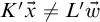
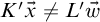


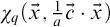














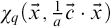


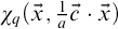


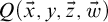







Now we verify that the above definitions are witnesses to the QETP.
-
(a) ( $\mathcal {L}$
is finite and closed under negation) Obvious. -
(b) ( $G\vDash \chi _{q}(\vec {x})\leftrightarrow (\exists \vec {y})q(\vec {x},\vec {y})$
) By construction. -
(c) There are two bullet points here. In reverse order:
-
• ( $G\vDash \chi _{q}(\vec {x})\land \varphi (\vec {x})\rightarrow (\exists y)\tau _{q\varphi }(\vec {x},y)$
) Direct from construction. -
• (Every tuple $\vec {b}$
of elements of G that satisfies
$\chi _{q}(\vec {b})$
satisfies some
$\varphi (\vec {b})$
with
$(q,\varphi )$
in domain of
$\tau $
)-
– If $\vec {b}=\vec {0}$
this is obvious. -
– If some $b_{i}\neq 0$
: We wish to show that there are
$a\in \mathbb {Z}_{\neq 0}$
and
$\vec {c}\subseteq \mathbb {Z}$
such that
$a\mid \vec {c}\cdot \vec {b}$
and
$\chi _{q}(\vec {b},\frac {1}{a}\vec {c}\cdot \vec {b})$
. To this effect, we use the following related lemma, which obviously implies the desired claim.Lemma 3.10. If $q(\vec {x},\vec {y})$
is a quantifier-free type in the smaller signature
$\mathcal {L}$
, and
$\vec {b}$
is a tuple in G such that
$G\vDash (\exists \vec {y})q(\vec {b},\vec {y})$
, and some element of
$\vec {b}$
is nonzero, then there exist integer vectors
$\vec {c}_{1},\dots ,\vec {c}_{\ell }$
and nonzero integers
$a_{1},\dots ,a_{\ell }$
such that, for every i,
$a_{i}\mid \vec {c}_{i}\cdot \vec {b}$
, and
$G\vDash q(\vec {b},\frac {1}{a_{1}}\vec {c}_{1}\cdot \vec {b},\dots ,\frac {1}{a_{\ell }}\vec {c}_{\ell }\cdot \vec {b})$
.The proof of this lemma uses a change of variables, similar to the one used in the construction of $\chi _{q}$
, followed by noticing Remark 3.9. The details are omitted.
-
-
-
(d) ( $G\vDash (\exists y)\left [\chi _{Q}(\vec {x},y)\land \tau _{q\varphi }(\vec {x},y)\right ]\leftrightarrow \varepsilon \tau _{q\varphi Q}(\vec {x})$
) True by construction. -
(e) ( $G\vDash \varepsilon \tau _{q\varphi Q}(\vec {x})\land \tau _{q\varphi }(\vec {x},y)\rightarrow \chi _{Q}(\vec {x},y)$
) Essentially, this is true because
$\tau _{q\varphi }(\vec {x},y)$
always determines y uniquely in terms of
$\vec {x}$
. As such, if it is the case that there is some
$y_{0}$
that satisfies
$\chi _{Q}(\vec {x},y_{0})\land \tau _{q\varphi }(\vec {x},y_{0})$
(i.e.,
$\varepsilon \tau _{q\varphi Q}(\vec {x})$
holds), and it is the case that some specific y satisfies
$\tau _{q\varphi }(\vec {x},y)$
, then it must be the case that
$y=y_{0}$
and therefore
$\chi _{Q}(\vec {x},y)$
.





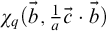


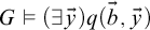











We are in condition to apply Theorem 2.6 to the
$0'$
 -computable c.e.-typed copy of G (plus designated element). Since this copy was obtained uniformly from the original presentation, the result is uniform.
4 Escaping Tennenbaum’s theorem with more truths
In this section, we give a positive answer to the question posed by Pakhomov in [Reference Pakhomov18], about whether there exist theories definitionally equivalent to “
$\mathsf {PA}$
 + all
$\Pi _{n}$
+ all
$\Pi _{n}$
 truths” that admit computable nonstandard models.
As described in the introduction, we will be working primarily with the theory
$\mathsf {ZF}\mathord {-}\mathsf {inf}\mathord {+}\mathsf {TC}$
 , which consists of the axioms of
$\mathsf {ZF}$
, which consists of the axioms of
$\mathsf {ZF}$
 , with the removal of the axiom of infinity, and with the addition of the axiom of transitive closure, which for our purposes is the axiom stating that every set is in some level
$V_{\alpha }$
, with the removal of the axiom of infinity, and with the addition of the axiom of transitive closure, which for our purposes is the axiom stating that every set is in some level
$V_{\alpha }$
 of the von Neumann hierarchy.
4.1 Generalizing Pakhomov’s construction
This section is dedicated to the proof of Theorem 4.1.
Theorem 4.1. There is a nested sequence of consistent c.e. theories
$\mathsf {ZF}\mathord {-}\mathsf {inf}\mathord {+}\mathsf {TC}\subseteq T^{0}\subseteq T^{1}\subseteq T^{2}\subseteq \cdots $
 satisfying the following properties:
-
• Each $T^{n}$
is in the signature containing
$\in $
and predicates
$S^{0}$
,
$\dots $
,
$S^{n}$
, with each
$S^{i}$
being an
$(i+2)$
-ary predicate symbol. -
• All of these extensions are conservative, in the sense that they contain no additional theorems in the predicate $\in $
. -
• The predicates $\in $
and
$S^{n}$
are definable in terms of the other within
$T^{n}$
. -
• Given an $X'$
-computable model D of
$T^{n}$
restricted to the signature containing
$S^{i}$
,
$\dots $
, and
$S^{n}$
, there is an X-computable copy M of
$D\mathord {\upharpoonright }(S^{i+1},\dots ,S^{n})$
.



We start the proof by defining the sequence
$\{T_{n}\}_{n\in \mathbb {N}}$
 inductively. For the base case, we set
$T^{0}$
inductively. For the base case, we set
$T^{0}$
 to be
$\mathsf {ZF}\mathord {-}\mathsf {inf}\mathord {+}\mathsf {TC}$
to be
$\mathsf {ZF}\mathord {-}\mathsf {inf}\mathord {+}\mathsf {TC}$
 , plus the axiom
$(\forall x,y)[S^{0}(x,y)\leftrightarrow (x\notin y)]$
, plus the axiom
$(\forall x,y)[S^{0}(x,y)\leftrightarrow (x\notin y)]$
 . It trivially (and, in the case of the last bullet point, almost vacuously) satisfies all required conditions. Now, we suppose that
$T^{n}$
. It trivially (and, in the case of the last bullet point, almost vacuously) satisfies all required conditions. Now, we suppose that
$T^{n}$
 has already been defined, and set out to define
$T^{n+1}$
has already been defined, and set out to define
$T^{n+1}$
 .
.
Within
$T^{n}$
 , we define the ordinal-indexed sequence of predicates
$S_{\alpha }^{n+1}(\vec {x},y)$
, we define the ordinal-indexed sequence of predicates
$S_{\alpha }^{n+1}(\vec {x},y)$
 , where
$\vec {x}$
, where
$\vec {x}$
 is an
$(n+1)$
is an
$(n+1)$
 -tuple of variables and
$\alpha $
-tuple of variables and
$\alpha $
 is an ordinal. We define
$S_{\alpha }^{n+1}$
is an ordinal. We define
$S_{\alpha }^{n+1}$
 inductively as a compatible sequence of relations on
$V_{\alpha }$
inductively as a compatible sequence of relations on
$V_{\alpha }$
 with
$S_{\lambda }^{n+1}$
with
$S_{\lambda }^{n+1}$
 having an obvious definition for limit ordinals
$\lambda $
having an obvious definition for limit ordinals
$\lambda $
 , so it suffices to describe the successor step. To assist us in that regard, we define the following sequence of class functions.
Given sets A,
$mA$
 , an ordinal
$\alpha $
, an ordinal
$\alpha $
 , and sets
$S^{i}A\subseteq (A\cup \{\alpha \})^{i+2}$
, and sets
$S^{i}A\subseteq (A\cup \{\alpha \})^{i+2}$
 for
$i=0,\dots ,n+1$
for
$i=0,\dots ,n+1$
 ,Footnote
9
define an element
$w^{n}(\alpha ,mA,A,SA,\dots ,S^{n}A)$
,Footnote
9
define an element
$w^{n}(\alpha ,mA,A,SA,\dots ,S^{n}A)$
 inductively in n as follows:
-
• $w^{0}(\alpha ,mA,A)=(\alpha ,(A,mA))$
, and -
• $w^{n+1}(\alpha ,mA,A,S^{0}A,S^{1}A,\dots ,S^{n}A,S^{n+1}A)=w^{n}(\alpha ,(S^{n+1}A,mA),A,S^{0} A,\dots ,S^{n}A)$
.


The main defining features of this sequence of class functions are:
-
• for every n, $(\alpha ,mA,A,S^{0}A,\dots ,S^{n}A)\mapsto w^{n}(\alpha ,mA,A,S^{0}A,\dots ,S^{n}A)$
is an injective definable class function, and -
• $w^{n}(\alpha ,mA,A,S^{0}A,\dots ,S^{n}A)$
is not in
$V_{\alpha }$
.



Let us go back to defining
$S_{\alpha }^{n+1}$
 inductively, assuming that we have already defined
$S^{0}$
inductively, assuming that we have already defined
$S^{0}$
 up to
$S^{n}$
up to
$S^{n}$
 , for
$n\geq 0$
, for
$n\geq 0$
 . Assuming that
$S_{\alpha }^{n+1}$
. Assuming that
$S_{\alpha }^{n+1}$
 is already defined on tuples of elements of
$V_{\alpha }$
is already defined on tuples of elements of
$V_{\alpha }$
 , we define a “good sequence”
$(\alpha ,mA,A,S^{0}A,\dots ,S^{n+1}A)$
, we define a “good sequence”
$(\alpha ,mA,A,S^{0}A,\dots ,S^{n+1}A)$
 as one that satisfies the following properties:
-
• A is a subset of $V_{\alpha }$
, -
• for $i=0,\dots ,n+1$
, the set
$S^{i}A$
is a subset of
$(A\cup \{\alpha \})^{i+2}$
, -
• for $i=0,\dots ,n$
, the set
$S^{i}A\cap A^{i+2}$
coincides with the relation
$S^{i}$
on A, -
• the set $S^{n+1}A\cap A^{n+3}$
coincides with the relation
$S_{\alpha }^{n+1}$
on A, -
• the set $S^{0}A$
contains all pairs
$(a,\alpha )$
,
$(\alpha ,a)$
, and
$(\alpha ,\alpha $
), with
$a\in A$
, and -
• for $i=0,\dots ,n$
, the following condition holds: For every
$(i+3)$
-tuple
$(\vec {a},b)$
of elements of
$A\cup \{\alpha \}$
, if
$\vec {a}\notin S^{i}A$
, then
$(\vec {a},b)\in S^{i+1}A$
.





We are now ready to define
$S_{\alpha +1}^{n+1}$
 . Given an
$(n+3)$
. Given an
$(n+3)$
 -tuple
$\vec {x}$
-tuple
$\vec {x}$
 of elements in
$V_{\alpha +1}$
of elements in
$V_{\alpha +1}$
 :
:
-
• If all elements of the tuple are in $V_{\alpha }$
, set
$S_{\alpha +1}^{n+1}(\vec {x})\equiv S_{\alpha }^{n+1}(\vec {x})$
. -
• If there is a good sequence $(\beta ,mA,A,S^{0}A,\dots ,S^{n+1}A)$
, for some
$\beta \leq \alpha $
, such that the element
$w=w^{n+1}(\beta ,mA,A,S^{0}A,\dots ,S^{n+1}A)$
is in
$V_{\alpha +1}$
, and every entry of
$\vec {x}$
is an element of
$A\cup \{w\}$
, set
$S_{\alpha +1}^{n+1}(\vec {x})$
to hold true if, and only if, upon replacing every instance of w in the tuple
$\vec {x}$
by
$\beta $
, the resulting tuple is in
$S^{n+1}A$
.In the sequence, when such a choice of good sequence is clear from context, denote by $\vec {x}^{*}$
the operation of replacing every entry of
$\vec {x}$
that equals
$\beta $
by w, and let
$\vec {x}_{*}$
denote the inverse operation. Thus, the definition of
$S_{\alpha +1}^{n+1}$
in this case can be reworded as:
$S_{\alpha +1}^{n+1}(\vec {x})\equiv [\vec {x}^{*}\in S^{n+1}A]$
.Remark: Note that, by definition, if $(\beta ,mA,A,S^{0}A,\dots ,S^{n+1}A)$
is a good sequence and
$n\geq 0$
, we also have that
$(\beta ,(S^{n+1}A,mA),A,S^{0}A,\dots ,S^{n}A)$
is also a good sequence (for a smaller value of n), and thus the element
$w=w^{n+1}(\beta ,mA,A,S^{0}A,\dots ,S^{n+1})=w^{n}(\beta ,(S^{n+1}A,mA),A,S^{0}A,\dots ,S^{n}A)$
will also satisfy:
$S^{n}(\vec {x})\equiv [\vec {x}^{*}\in S^{n}A]$
for all tuples of elements of
$A\cup \{w\}$
, and inductively for lower indices. The case of
$S^{0}$
is an edge case, but the definition of good sequence still ensures that
$S^{0}(x,y)\equiv [(x,y)^{*}\in S^{0}A]$
. -
• For every other triple of elements from $V_{\alpha +1}$
, set
$S_{\alpha +1}^{n+1}(\vec {x})$
to hold true.


















Note that the first and second item in the definition do not contradict each other: If a tuple
$\vec {x}$
 fits both bullet points, then either all its elements are in A, in which case the definition of good sequence ensures that there is agreement between both possible definitions of
$S_{\alpha +1}^{n+1}(\vec {x})$
fits both bullet points, then either all its elements are in A, in which case the definition of good sequence ensures that there is agreement between both possible definitions of
$S_{\alpha +1}^{n+1}(\vec {x})$
 , or one of its elements is
$w=w^{n+1}(\beta ,mA,A,\dots ,S^{n+1}A)$
, or one of its elements is
$w=w^{n+1}(\beta ,mA,A,\dots ,S^{n+1}A)$
 , in which case
$S_{\gamma }^{n+1}(\vec {x})$
, in which case
$S_{\gamma }^{n+1}(\vec {x})$
 would have been defined to agree with the second bullet point for
$\gamma $
would have been defined to agree with the second bullet point for
$\gamma $
 the smallest ordinal such that
$w\in V_{\gamma }$
the smallest ordinal such that
$w\in V_{\gamma }$
 .
.
This induces a well-defined relation
$S^{n+1}$
 , whose main defining properties are as follows.
Lemma 4.2. Provably in
$\mathsf {ZF}\mathord {-}\mathsf {inf}\mathord {+}\mathsf {TC}$
 ,
$\neg S^{n}(\vec {x})$
,
$\neg S^{n}(\vec {x})$
 iff
$(\forall y)S^{n+1}(\vec {x},y)$
iff
$(\forall y)S^{n+1}(\vec {x},y)$
 .
.
Proof. By construction.
Lemma 4.3. Let M be a model of
$\mathsf {ZF}\mathord {-}\mathsf {inf}\mathord {+}\mathsf {TC}$
 . Let A be a finite subset of M, and suppose that we wish to find an element w that relates to all elements of A with regard to the predicates
$S^{0},\dots ,S^{n+1}$
. Let A be a finite subset of M, and suppose that we wish to find an element w that relates to all elements of A with regard to the predicates
$S^{0},\dots ,S^{n+1}$
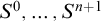 in a prescribed manner. The following is a sufficient condition for there to exist an element w of M satisfying this prescription: For every
$0\leq i\leq n$
in a prescribed manner. The following is a sufficient condition for there to exist an element w of M satisfying this prescription: For every
$0\leq i\leq n$
 , the prescription satisfies the rules:
-
• The prescription agrees with the pre-existing relations on tuples that don’t contain any instance of w.
-
• For all $x\in A\cup \{w\}$
, it is prescribed that
$S^{0}(x,w)$
and
$S^{0}(w,x)$
. -
• For all $(\vec {x},y)\in (A\cup \{w\})^{i+2}$
such that
$\neg S^{i}(\vec {x})$
is prescribed, it is also prescribed that
$S^{i+1}(\vec {x},y)$
.



Proof. By construction.
These two properties are enough to establish the following theorem.
Theorem 4.4. Let D be an
$X'$
 -computable model of
$T^{n}$
-computable model of
$T^{n}$
 in the predicates
$S^{i},\dots ,S^{n}$
in the predicates
$S^{i},\dots ,S^{n}$
 , with
$i<n$
, with
$i<n$
 . Then, the reduct
$D\mathord {\upharpoonright }(S^{i+1},\dots ,S^{n})$
. Then, the reduct
$D\mathord {\upharpoonright }(S^{i+1},\dots ,S^{n})$
 admits an X-computable copy.
Proof. We will apply Theorem 2.6 to D which, as an
$X'$
 -computable model over a finite signature, is also an
$X'$
-computable model over a finite signature, is also an
$X'$
 -computable X-c.e.-typed model. We need only establish that D has the QETP over
$\mathcal {L}=(S^{i+1},\dots ,S^{n})$
-computable X-c.e.-typed model. We need only establish that D has the QETP over
$\mathcal {L}=(S^{i+1},\dots ,S^{n})$
 (plus negations) and
$\mathcal {L}'=(S^{i},\dots ,S^{n})$
(plus negations) and
$\mathcal {L}'=(S^{i},\dots ,S^{n})$
 (plus negations).
We construct
$\chi $
 ,
$\tau $
,
$\tau $
 , and
$\varepsilon \tau $
, and
$\varepsilon \tau $
 :
:
-
• First, we construct $\chi _{q}$
for
$q(\vec {x},\vec {y})$
a quantifier-free
$\mathcal {L}$
-type with all variables distinct.We start by considering the case, where $q(\vec {x},y)$
only has one y-variable. In this case, the formula
$(\exists y)q(\vec {x},y)$
is true if, and only if, there exists an element y satisfying a certain prescription of predicates
$S^{i+1},\dots ,S^{n}$
. We show that the following three statements are equivalent:-
– $P(\vec {x})\equiv (\exists y)q(\vec {x},y)$
-
– $Q(\vec {x})$
: For every instance of
$\neg S^{j+1}(\vec {z}_{0},z_{1})$
in
$q(\vec {x},y)$
:-
* if $j>i$
, we require that
$S^{j}(\vec {z}_{0})$
be in q, andFootnote
10
-
* if $j=i$
,
$z_{1}\equiv y$
, and
$\vec {z}_{0}$
is a subtuple of
$\vec {x}$
, we require
$S^{i}(\vec {z}_{0})$
.
Moreover, we also demand $(q\mathord {\upharpoonright }\vec {x})(\vec {x})$
. In other words, whatever demand q makes of the tuple
$\vec {x}$
, we also demand it. -
-
– $R(\vec {x})\equiv $
There is a y such that
$q(\vec {x},y)$
and the relations
$S^{0}$
to
$S^{i}$
hold for all tuples including elements from
$(\vec {x},y)$
that include at least one instance of y.
Indeed, $P(\vec {x})\rightarrow Q(\vec {x})$
follows from the fact that
$(\forall \vec {z}_{0})((\exists z_{1})\neg S^{j+1}(\vec {z}_{0},z_{1}))\rightarrow S^{j}(\vec {z}_{0})$
(and the assumption that q is a type),
$Q(\vec {x})\rightarrow R(\vec {x})$
follows by Lemma 4.3, and
$R(\vec {x})$
obviously implies
$P(\vec {x})$
.Now, still in the case where there is only one y-variable, we set $\chi _{q}(\vec {x})\equiv Q(\vec {x})$
as above. We will now handle the case where there are two y-variables, say
$y_{1}$
and
$y_{2}$
, and an obvious induction will handle the general case. We will use the formulas P, Q, and R constructed above for different formulas q. We will use a subscript to indicate which formula q is being used.Let $q(\vec {x},y_{1},y_{2})$
be a quantifier-free
$\mathcal {L}$
-type. Then, let us look at
$\chi _{q}(\vec {x},y_{1})$
. As above, it’s either
$\bot $
(if the first bullet point of the definition of
$Q_{q}(\vec {x},y_{1})$
fails), in which case the quantifier elimination is trivial, or otherwise it consists of
$q\mathord {\upharpoonright }(\vec {x},y_{1})$
, together with a few positive requirements of type
$S^{i}(\vec {z}_{0})$
with
$\vec {z}_{0}$
a subtuple of
$(\vec {x},y_{1})$
. Let
$q'(\vec {x},y_{1})$
be
$q\mathord {\upharpoonright }(\vec {x},y_{1})$
together with those requirements that include
$y_{1}$
, and
$q^{*}(\vec {x})$
be the remainder of these requirements. Note that $$\begin{align*}(\exists y_{1})(\exists y_{2})q(\vec{x},y_{1},y_{2})\leftrightarrow(\exists y_{1})\chi_{q}(\vec{x},y_{1})\leftrightarrow q^{*}(\vec{x})\land(\exists y_{1})q'(\vec{x},y_{1}), \end{align*}$$and crucially that, since all $S^{i}$
-requirements made by
$q'$
are positive,
$(\exists y_{1})q'(\vec {x},y_{1})$
is logically between
$P_{q'}(\vec {x})$
and
$R_{q'}(\vec {x})$
, and as such is equivalent to both, and as such is equivalent to
$Q_{q'}(\vec {x})$
. Then, we conclude
$(\exists \vec {y})q(\vec {x},\vec {y})\leftrightarrow q^{*}(\vec {x})\land Q_{q'}(\vec {x})$
, and so we define the latter as
$\chi _{q}$
in this scenario. The induction continues in a similar fashion, in the event that there are more y-variables, with the essential point being that every
$S^{i}$
-demand being made at any step is positive.
-
-
• Now, we construct $\tau $
. Given
$q(\vec {x},y,\vec {z})$
, we set
$\tau _{q\top }(\vec {x},y)$
to be the demand that every
$S^{i}$
-relation including y at least once holds, and that
$\chi _{q}(\vec {x})$
holds. -
• Finally, $\varepsilon \tau _{q\top Q}(\vec {x})$
is simply
$\chi _{Q}(\vec {x})$
.




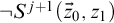
















The proof that these formulas are witnesses to the QETP is simple and follows the same P, Q, and R reasoning used to establish that
$\chi _{q}(\vec {x})\leftrightarrow (\exists y)q(\vec {x},y)$
 .
.
Theorem 4.1 immediately follows.
As explained in the introduction, we obtain as a corollary.
Theorem 4.5. For every n, there is a theory definitionally equivalent to “
$\mathsf {PA}$
 plus all true
$\Pi _{n}$
plus all true
$\Pi _{n}$
 sentences” that has a computable nonstandard model.
5 Further questions
It is a standard theorem (or definition) that a
$\mathrm {PA}$
 degree is the same as one which computes a nonstandard model of
$\mathsf {PA}$
degree is the same as one which computes a nonstandard model of
$\mathsf {PA}$
 . On the other hand, we saw that there is a computable nonstandard model of the definitionally equivalent theory
$T_{0}$
. On the other hand, we saw that there is a computable nonstandard model of the definitionally equivalent theory
$T_{0}$
 constructed by Pakhomov—and so, by a theorem of Knight [Reference Knight12], there exists one in every degree. Let us define, for a theory T that is definitionally equivalent to
$\mathsf {PA}$
constructed by Pakhomov—and so, by a theorem of Knight [Reference Knight12], there exists one in every degree. Let us define, for a theory T that is definitionally equivalent to
$\mathsf {PA}$
 , its nonstandard spectrum as the set of degrees of nonstandard models of T.
Question 1. If T is a c.e. theory that is definitionally equivalent to
$\mathsf {PA}$
 , we can see that its nonstandard spectrum is at most the set of all Turing degrees, and at least the set of all
$\mathrm {PA}$
, we can see that its nonstandard spectrum is at most the set of all Turing degrees, and at least the set of all
$\mathrm {PA}$
 degrees. Does there exist such a theory whose nonstandard spectrum is strictly in-between these two cases? More generally, what can the nonstandard spectrum of a c.e. theory definitionally equivalent to
$\mathsf {PA}$
degrees. Does there exist such a theory whose nonstandard spectrum is strictly in-between these two cases? More generally, what can the nonstandard spectrum of a c.e. theory definitionally equivalent to
$\mathsf {PA}$
 look like?
The methods used in this article are too coarse to address this question; they would have to be cleverly modified to stop the nonstandard spectrum from including
$0$
 .
.
We mentioned in the introduction that Lutz and Walsh [Reference Lutz and Walsh13] produced a c.e. consistent theory such that no definitionally equivalent theory has a computable model. In fact, they defined, for each infinite computable binary branching tree R with no “guessable” path, a consistent theory
$T_{\mathrm {LW}}(R)$
 such that no theory definitionally equivalent to
$T_{\mathrm {LW}}(R)$
such that no theory definitionally equivalent to
$T_{\mathrm {LW}}(R)$
 has a computable model. We wonder how close such models are to being computable.
Question 2. Define the Lutz–Walsh spectrum of an infinite computable binary tree R none of whose paths are guessable, say
$\mathrm {LWSpec}(R)$
 , as the set of Turing degrees that compute a model of a theory definitionally equivalent to
$T_{\mathrm {LW}}(R)$
, as the set of Turing degrees that compute a model of a theory definitionally equivalent to
$T_{\mathrm {LW}}(R)$
 . It is clear that this
$\mathrm {LWSpec}(R)$
. It is clear that this
$\mathrm {LWSpec}(R)$
 always contains all
$\mathrm {PA}$
always contains all
$\mathrm {PA}$
 degrees, and in [Reference Lutz and Walsh13] it is proven that
$\mathrm {LWSpec}(R)$
degrees, and in [Reference Lutz and Walsh13] it is proven that
$\mathrm {LWSpec}(R)$
 does not contain
$0$
does not contain
$0$
 (if, again, none of the paths of R are guessable). Does
$\mathrm {LWSpec}(R)$
(if, again, none of the paths of R are guessable). Does
$\mathrm {LWSpec}(R)$
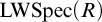 ever contain any degrees that are not
$\mathrm {PA}$
ever contain any degrees that are not
$\mathrm {PA}$
 ? If so, how far from
$\mathrm {PA}$
? If so, how far from
$\mathrm {PA}$
 can we get? Is there such a tree R for which
$\mathrm {LWSpec}(R)$
can we get? Is there such a tree R for which
$\mathrm {LWSpec}(R)$
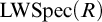 consists of all nonzero degrees? Is there any nonzero degree that can never be in
$\mathrm {LWSpec}(R)$
consists of all nonzero degrees? Is there any nonzero degree that can never be in
$\mathrm {LWSpec}(R)$
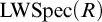 ?
?
In the statement of Theorem 4.1, the arity of the predicate used to replace set inclusion increased by
$1$
 for every jump in complexity. We wonder if this is a logical necessity or merely an artifact of our construction.
Question 3. For a given value of n, does there exist a theory
$T_{Q}^{n}$
 , axiomatizing a single ternary predicate
$Q(x,y,z)$
, axiomatizing a single ternary predicate
$Q(x,y,z)$
 , such that
$T_{Q}^{n}$
, such that
$T_{Q}^{n}$
 is definitionally equivalent to “
$\mathsf {PA}$
is definitionally equivalent to “
$\mathsf {PA}$
 plus all
$\Pi _{n}$
plus all
$\Pi _{n}$
 truths” which admits a computable nonstandard model? What if we require the predicate to be binary, instead?
While Theorem 2.6 guarantees the existence of a
$0'$
 -computable isomorphism between the original structure and its computable copy, most results in the literature can only guarantee (out of necessity) a
$0"$
-computable isomorphism between the original structure and its computable copy, most results in the literature can only guarantee (out of necessity) a
$0"$
 or
$0"'$
or
$0"'$
 -computable isomorphism. This is explained by the fact that, in our proofs, we must first create a
$0'$
-computable isomorphism. This is explained by the fact that, in our proofs, we must first create a
$0'$
 -computable c.e.-typed copy which is isomorphic to the original structure, though this isomorphism may itself need to be complex. Hirschfeldt asked whether one could obtain a more direct result, for example, by weakening the assumptions of the QETP.
Question 4 (Hirschfeldt)
Does there exist a version of Theorem 2.6 that requires weaker assumptions, possibly using an infinite injury method instead of finite injury, from which theorems, such as Theorem 3.1 (jump inversion for linear orders) or Proposition 3.2 (jump inversion for equivalence relations with infinitely many infinite classes) may be obtained more easily?
Many general results in computable structure theory necessitate the use of a finite relational signature, oftentimes for reasons similar to those that led us to the notion of
$0'$
 -computable c.e.-typed structure. We wonder if our definition would be applicable to other scenarios.
Question 5. Are there results in the literature, applicable to finite relational signatures, which could be further (and usefully) generalized using the notion of
$0'$
 -computable c.e.-typed structure?
In Section 2.1, we found it useful to work with
$\bigvee\mathchoice{\hspace{-1.1em}}{\hspace{-0.7em}}{\hspace{-0.7em}}{\hspace{-0.6em}}\bigvee^{\mathrm {c}}$
 formulas, which are related to but not exactly the same as
$\Sigma _{1}^{\mathrm {c}}$
formulas, which are related to but not exactly the same as
$\Sigma _{1}^{\mathrm {c}}$
 formulas. Ash, Knight, Manasse, and Slaman showed that the definability of a relation by a
$\Sigma _{1}^{\mathrm {c}}$
formulas. Ash, Knight, Manasse, and Slaman showed that the definability of a relation by a
$\Sigma _{1}^{\mathrm {c}}$
 formula is related to computability-theoretic properties, namely, the notion of being a r.i.c.e. (relatively intrinsically c.e.) relation (see [Reference Montalbán16, Theorem II.16] for details). We wonder if
$\bigvee\mathchoice{\hspace{-1.1em}}{\hspace{-0.7em}}{\hspace{-0.7em}}{\hspace{-0.6em}}\bigvee^{\mathrm {c}}$
formula is related to computability-theoretic properties, namely, the notion of being a r.i.c.e. (relatively intrinsically c.e.) relation (see [Reference Montalbán16, Theorem II.16] for details). We wonder if
$\bigvee\mathchoice{\hspace{-1.1em}}{\hspace{-0.7em}}{\hspace{-0.7em}}{\hspace{-0.6em}}\bigvee^{\mathrm {c}}$
 formulas admit a similar treatment.
Question 6. Is there a computability-theoretic characterization of those relations in a structure that are definable by a
$\bigvee\mathchoice{\hspace{-1.1em}}{\hspace{-0.7em}}{\hspace{-0.7em}}{\hspace{-0.6em}}\bigvee^{\mathrm {c}}$
 formula?
Acknowledgments
I would like to thank Denis Hirschfeldt, Miles Kretschmer, and Patrick Lutz for their valuable feedback, help, and advice, without which this work would not have been possible.


 Open access

