

Introduction
A linkage exists between glacial hydrology and glacier sliding. The linkage is manifested in the concurrence of periods of high water pressure measured in boreholes and high sliding velocity (Reference Iken and Truffer.Iken and Truffer, 1997), in pulses of turbidity associated with “mini-surge” behavior at Variegated Glacier, Alaska, U.S.A. (Reference Humphrey, Raymond. and Harrison.Humphrey and others, 1986), in coincident increases in suspended-sediment concentration and straining on the ice of Black Rapids and Fels Glaciers, Alaska (Reference Raymond, Benedict., Harrison., Echelmeyer. and Sturm.Raymond and others, 1995), and in the correlation between large water inputs from melt or rain and rapid sliding at Storglaeiären, Sweden (Reference Hooke, Calla., Holmlund., Nilsson. and Stroeven.Hooke and others, 1989; Reference JanssonJansson, 1996). High basal water pressures expand the size of cavities at the bed, which reduces the area of frictional coupling at the bed and reduces effective stresses (Reference Iken and Bindschadler.Iken and Bindschadler, 1986). Subglacial water also exerts a down-glacier force on the ice that drives sliding, an effect likely to depend on the volume of stored water (Reference HumphreyHumphrey, 1987). Work on Columbia Glacier, Alaska (Reference Kamb, Engelhardt., Fahnestock., Humphrey., Meier. and Stone.Kamb and others, 1994; Reference MeierMeier and others, 1994), has suggested that because the water-pressure field at the bed may be highly localized, a better surrogate for the role of water in modulating glacier sliding may be the water storage at the bed. At Unteraargletscher, Switzerland, Reference Iken, Röthlisberger, Flotron. and Haeberli.Iken and others (1983) correlated maximum upward movement rates with maximum sliding velocities, and inferred that the uplift was accommodating water storage at the bed.
Understanding the intimate coupling between the hydrological state and sliding-rate pattern of a glacier should provide insight into the controls on subglacial abrasion and quarrying, both of which require sliding. In addition, as water chemistry in the glacial system is coupled to the pathways and residence times within various reservoirs that include the subglacial cavity system, the chemistry of the glacier outlet stream can potentially be used as a probe of the system (Reference Tranter, Brown., Raiswell., Sharp. and Gurnell.Tranter and others, 1993; Reference CollinsCollins, 1995; Reference Brown, Sharp. and Tranter.Brown and others, 1996b).
Brief (non-surge) episodes of high sliding velocities can occur in any part of the melt season and in any part of the glacier. In spring, the subglacial hydrologic system is thought to undergo a progressive reorganization from one dominated by a distributed flow system to one with conduits that can efficiently transmit meltwater to the terminus (Reference Fountain and Walder.Fountain and Walder, 1998; Reference Hubbard and Nienow.Hubbard and Nienow, 1998). Here, we present observations of a spring speed-up and flood event at Bench Glacier, Alaska, in which several lines of evidence suggest that the formation of conduits occurs forcefully when the distributed system is overwhelmed by meltwater inputs. We collected data in June, early in the melt season, when this subglacial reorganization is likely to be occurring close to the terminus of the glacier, and hence its manifestations in the outlet stream are not diffused by long travel distances. Importantly, since the flood event we recorded followed 9 days of clear weather, it cannot be attributed to storm input. In addition to measuring ice velocity, snowmelt, water discharge and sediment concentration, we made detailed observations of the chemistry of the outlet stream.
Field Site and Methods
Bench Glacier, in the Chugach Mountains of south-central Alaska (Fig. 1), is comparable in size to the well-studied Worthington Glacier 12 km to the north (Reference Harper, Humphrey., Pfeffer. and Welch.Harper and others, 1996, Reference Harper, Humphrey. and Pfeffer.1998a, Reference Harper, Humphrey. and Pfeffer.b; Reference Welch, Pfeffer., Harper. and Humphrey.Welch and others, 1998). Its present footprint of 9.0 km2 is remarkably simple in plan. Bench Glacier has no tributaries and, with the exception of one ice-fall, slopes fairly uniformly at 10° until within approximately 1 km of its terminus. The present terminus is at an elevation of 945 m (3100 ft), and the headwall is surrounded by peaks up to 2151m (7057 ft). The total basin area above our gauge is 12.5 km2. The single outlet stream yields maximum discharges of order 10 m3 s1. The glacier is therefore well suited for a variety of investigations, including those that rely upon capturing the discharges of both water and sediment using simple field instrumentation methods.
Map of Bench Glacier. Contours are 500ft (152 m), and spot elevations are in feet. Drainage divide is dashed, showing nearly full occupation of the valley area by ice except for recently deglaciated small cirque near the terminus on glacier-right. Detail of the terminus area includes the gauging station (G), the survey station (open triangle) and the two reflectors on the ice surface (filled dots), all of which are shown in cross-section in the bottom left inset. Comparison of the 1950 terminus, from the USGS Valdez (A-5) 15’ quadrangle, and the 1996 terminus documents roughly 20 m a−1 of retreat. Stream-gauge set-up is shown in upper right inset, including tethered “fish”, boom supporting acoustic sensor for stream stage, and data-logger box in which box temperature was logged as well.
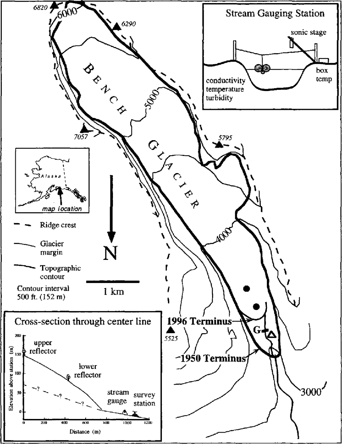
The present terminus of Bench Glacier is 2–2.5 km back from its Little Ice Age (LIA) terminus position. Although the timing of the LIA maximum has not been established at Bench Glacier, it is likely to be similar to the history on the west side of Prince William Sound, where tree-ring chronologies show that two glacier culminations of nearly equal size occurred in AD 1710 and AD 1870–1900 (Reference CalkinCalkin, 1988; Reference Barclay and Calkin.Barclay and Calkin, 1996). Bench Glacier has retreated 800 m since 1950, when the aerial photography for the U.S. Geological Survey (USGS) topographic map (Valdez A-5, 1: 63 360) was done. These observations yield average modern retreat rates of 20 m−1.
The glacier is underlain by late-Cretaceous age meta-sediments of the Valdez Group (Reference Winkler, Silberman., Grantz., Miller. and MacKevett.Winkler and others, 1981; Reference Plafker, Nokleberg. and Lull.Plafker and others, 1989). Bedrock docs not crop out on the proglacial valley floor, but does appear in isolated outcrops low on the valley walls. Gullies cut into the valley walls attain depths of up to 3 m entirely within glacial till; this suggests that a subglacial till layer of at least this thickness occurs under the glacier itself.
We visited Bench Glacier for 16 days in June 1996. During that time, we monitored ice velocity, stream discharge, suspended-sediment concentration, water chemistry, air temperature and snowmelt rates. At the beginning of the period, no ice was visible on the glacier; on the last day, the snowline was at 1370 m (4500 ft), and roughly 30% of the glacier was snow-free.
Ice velocity
We used an isolated, 20 m tall moraine hill located near the center of the Bench Glacier valley, 300 m from the present terminus, as a base for observations of glacier motion (Fig. 1). This location afforded a line of sight up the center of the glacier, parallel to the expected ice-flow direction. A total station survey instrument (HP-3810B medium range) was set up on the moraine hill, and remained in place for the entire field visit. Two triple reflectors were installed on the ice approximately 663 and 1062 m from the station. Because the viewing angle was closely aligned with the flow direction, displacements of the reflectors toward the total station are interpreted directly as ice displacements. The reflectors were mounted on small sections of drill rod augered into the ice surface. Distances to the reflectors were measured at irregular intervals ranging from a few minutes to a few hours. The reflector poles were re-augered once, and were still firmly in their narrow holes when we departed. Given the time of our visit, we could measure distances in all but a few hours of the day, limited only by very late night darkness and occasional dense clouds.
Stream gauge
While the Bench River is braided close to the terminus, it becomes a moderately stable single thread incised into its banks by about 1 m where it crosses the moraine on which the total station was located. We installed a stream gauge, similar in design to that of Reference Humphrey, Raymond. and Harrison.Humphrey and others (1986), consisting of an acoustic water-stage sensor and surface-water conductivity, turbidity and temperature sensors. During the highest discharges, we defeated the stream’s pernicious attempts to braid upstream and divert flow around the gauging station by placing numerous boulders at the sites of breaches. Our minor modifications were sufficient to cause deposition by the channel at these spots, and keep the course unchanged past our gauge. At the most, a few per cent of the total flow leaked around the gauge at the highest discharge.
The temperature-compensated acoustic water-stage sensor (Lundahl) was cantilevered above the water surface with polyvinyl chloride (PVC) pipes. Each stage measurement consisted of an average of 100 readings in a 10 s period to reduce the noise associated with unsteady roughness of the water surface. Stage was recorded by a Campbell CR-10 data logger every 15 min.
Water temperature, electrical conductivity and turbidity were measured with a floating instrument package (Fig. 1, upper right inset). The instruments were banded to the bottom of a raft constructed of two sealed PVC pipes filled with closed-cell foam. The package was tethered to a steel cable across the river, and floated near the center of the flow for the first 10 days of the field visit. The cable failed upon collapse of the right bank, and thereafter, the package was tethered within 0.5 m of the left bank. The conductivity time series was much less noisy when the package was floating in the less turbulent water near the bank. The turbidity and conductivity signals did not show any other changes attributable to moving the sensors out of the channel talweg.
The turbidity sensor, patterned after Reference Stone, Clarke. and Blake.Stone and others (1993) and Reference Humphrey and Raymond.Humphrey and Raymond (1994), measures light intensity after passage across a 10 mm water-filled gap from a light-emitting diode (red) source. Ambient light is blocked by a series of black PVC baffles on either side of the measurement section of the tube, and water is allowed to pass through the tube. We found the sensor worked best when the baffles were oriented vertically, reducing the likelihood of accumulation of sediment within the tube as the flow is forced from side to side. Coarse sediment is prevented from entering the tube by a screen at the upstream end of the tube.
Water temperature was measured using a thermistor, and conductivity was measured using a commercial conductivity probe, both of which were attached to the turbidity sensor body.
Discharge rating curve
We used the salt-dilution method (Reference Kilpatrick and Cobb.Kilpatrick and Cobb, 1984; Reference KiteKite, 1994) or current-meter and channel cross-sectional area measurements to establish the discharge at 13 stages corresponding to the full range of discharges we witnessed. The salt-dilution method entailed injection of 1–2 kg of salt dissolved in 20 L of stream water, and measurement of time series of conductivity in the stream 100 m downstream. As the channel was typically 5–8 m wide, this distance was more than the recommended 6–10 channel widths (Reference KiteKite, 1994) necessary to ensure full mixing of the salt. The baseline conductivity, Ψ0, was established before salt injection, and we recorded data until we were confident that the flow had retained this baseline. The time series, Ψ(t), was collected at 5 s time-steps to ensure sufficient detail to obtain well-constrained integrals of the conductivity signal. We have done repeated salt discharge measurements elsewhere that suggest that errors in the deduced discharges are only a few per cent. The conductivity, Ψ, was related to salt concentration through C = bΨ, where the constant b = (1 kg m3) / (214 μs mm−1). Discharge was then calculated from the mass-balance relationship,
where M s is the mass of salt injected, and the time interval t = 0–T for the integral is that required for the entire salt wave to pass the observation station, i.e. for the conductivity signal Ψ(t) to return to the background value, Ψ0.
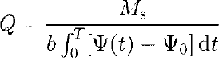
The rating curve (Fig. 2) is constructed using the acoustic-stage measurement nearest the time of discharge measurement. The two discharge measurements at the lowest acoustic stages fall off the linear trend defined by the other data points. These two measurements were made on 26 June, after a flood event (Fig. 3). We believe that the difference between these two points and the rest of the data is real; they are consistent with the shift expected for aggradation of the bed. We therefore used two rating curves, switching from the pre-26 June curve at 1315 h on 26 June, shortly before our discharge measurements that day, at the beginning of a 90 mm rise of the water surface in 75 min, the most rapid rise we recorded (Fig. 3). The resulting discharge curve varies smoothly across the switch in rating curves, instead of displaying the sharp jump on 26 June seen in the stage record (Fig. 3). Although the shifted rating curve is based on only two measurements, and therefore is not as well characterized as the pre-26 June curve, failure to make this adjustment results in calculated discharges that are greater than any of our measurements (i.e. constitutes an extrapolation rather than an interpolation of our data). In particular, discharges calculated using the pre-26 June rating curve exceed our measurements on 26 June by nearly 3 m3s1.
Discharge rating curves. Acoustic stage is distance from sensor down to the water surface, and hence varies inversely with discharge. Horizontal error bars are ±1σ for the acoustic-stage measurements, which are averages of 100 readings over 10 s. Vertical error bars are ± 10%. Data for 26 June (open circles) were collected after the spring flood event. Differences in the two curves reflect aggradation of the bed.
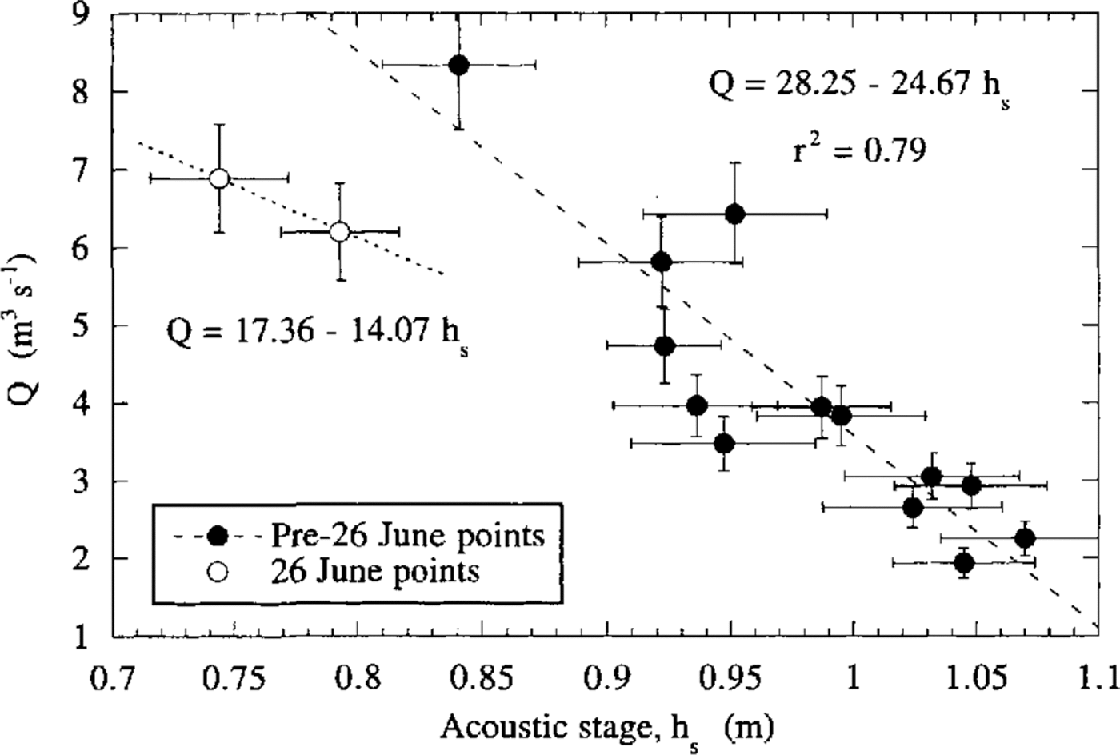
Stage and discharge records. Lower curve shows acoustically measured stage, plotted with y axis reversed, while upper set of curves shows calculated discharge (black) and± 1σ based on noise in acoustic-stage data (gray). Discharge measurements are shown with open circles. The last two discharge measurements, on 26 June, were accommodated only by switching to a new rating curve (Fig. 2). The shift in rating curves was applied at the beginning of the large step in acoustic stage at midday on 26 June, and results in calculated discharge showing a falling trend for observations after the 24 June peak.
Errors in our rating curve and discharge measurements are greatest at high discharge. Acoustic stages around 0.9 m associated with the onset of the 24 June flood were especially noisy at the measurement site, because the flow generated standing waves many cm in amplitude. If the time for a standing wave to pass the sensor location is different than the 15 min measurement frequency, then a single measurement could misrepresent the mean flow significantly, in either direction. The errors are as large as 1 m3 s−1 at the high flows (Fig. 3). In addition, the roughness of the water surface during any 10 s measurement contributes noise of ± 15 mm to the stage measurement, the effect of which is shown by the gray lines in Figure 3. Finally, our salt-dilution and current-meter measurements of discharge are not without error.
Suspended-sediment rating curve
Water samples were collected twice daily in 250 mL polyethylene bottles at the surface of the stream for solute and suspended-sediment analysis (Reference Østrem, Jopling and McDonald.Østrem, 1975). When the floating instrument package with the turbidity sensor was located close to the channel bank, these samples were collected within 0.5 m of the sensor. For most of the study, however, water samples were collected 2–5 m from the turbidity sensor, usually slightly upstream. Samples were vacuum-filtered through 0.45 μm filters (Gelman Metricel) in the field. Although the filters were not pre-weighed, variability between blank filters amounted to just ±1.2 mg (1.6%). Seven aliquots were collected within a period of 1 min on 20 June to test reproducibility; the mean and standard-deviation concentration of these was 2223 ±54 mg L−1.
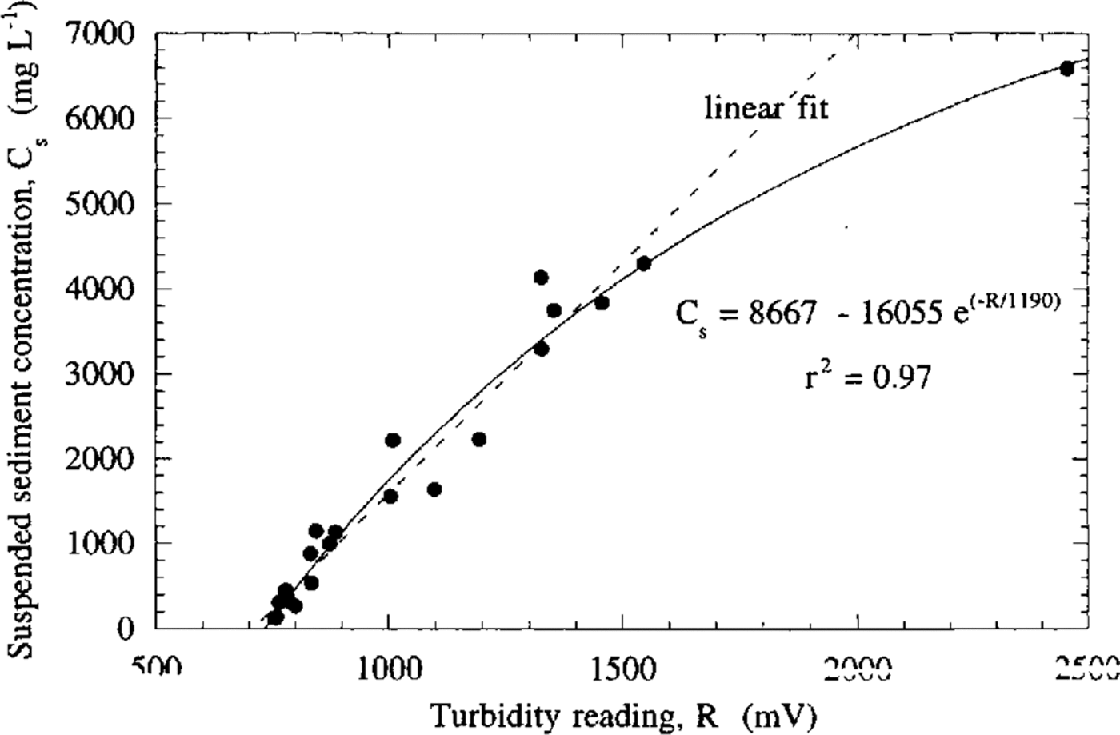
The suspended-sediment rating curve (Fig. 4) is nearly linear over much of its range, but this relationship falls off at turbidity readings of > 1500 mV. To be conservative, we used the exponential fit shown in Figure 4, which is similar to the empirical fit used by Reference Humphrey, Raymond. and Harrison.Humphrey and others (1986). The turbidity sensor readings were pinned at the top of its range, 2500 mV, during the peak discharges of the spring flood; calculated concentrations during these times therefore are likely to underestimate the suspended-sediment concentration.
Suspended-sediment rating curve. Uppermost data point is close to turbidity-sensor saturation value of 2500 mV. The exponential fit was adopted for suspended-sediment calculations because it is more conservative at high turbidity readings than the linear curve shown.
The turbidity sensor is attached to the base of the PVC floats, and is therefore very near the surface of the flow, where sediment grain-size and concentration are at a minimum. In order to assess the degree to which this measurement underestimates the mean concentration, we measured one sediment-concentration profile (Fig. 5), collected on 20 June by attaching four bottles to a dowel. For suspended-sediment transport, one expects (e.g. Reference RouseRouse, 1937) a power-law relationship between concentration, C, and depth, z, i.e. C = C a(z/z a)p, where C a is the measured concentration at a reference height z a above the bed, and the exponent is the Rouse number, p = w/(ku *), where w is the settling velocity of the grains in suspension, k is von Kármán’s constant (0.4) and u * is the shear velocity of the flow ((gHS)1/2, where H is flow depth and S is channel slope). The sediment concentration indeed increases significantly with depth (Fig. 5), and the profile may be approximated by a power law with exponent –0.39. For the local slope of the channel (0.04), and instantaneous flow depth of 0.29 m, we expect u * = 0.34 m s−1. Solving for settling velocity from the Rouse number, w = pku *, we find that the settling velocity of the sediment dominating the concentration profile is 0.05 m s−1. From settling-velocity relationships (e.g. Reference DietrichDietrich, 1982), this corresponds to quartz grains of diameter roughly 10−4 m, or coarse silt, a reasonable prediction for the dominant sediment in suspension in this glacial river. The ratio of the surface concentration, C s, to die mean (vertically averaged) concentration, ![]() , is
, is
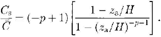
For our case, with P = 0.39, Equation (2) suggests that this ratio should be 0.8, meaning that by measuring the surface concentration, our measurements reflect roughly 80% of the mean suspended-sediment concentration. We have not corrected our suspended-sediment concentrations, calculated from our turbidity time series, for this effect. Nor have we quantified transport by bedload, which can be up to 50% of the sediment discharge by a glacial stream (Reference Church, Gilbert., Jopling and McDonald.Church and Gilbert, 1975; Reference Østrem, Jopling and McDonald.Østrem, 1975; Reference Hammer and Smith.Hammer and Smith, 1983; Reference Gomez, Gurnell and Clark.Gomez, 1987) and is not treated by the suspended-sediment transport analysis above. Rather, the surface concentration we use to constrain the mean concentration should be considered lower-bound estimates.
Suspended-sediment concentration profile showing strong concentration gradient within the flow. Samples taken from a sampling rod to which four bottles were attached at regular intervals, all opened to the flow once the rod was in place. A simple power law fits the data well, with a Rouse number of 0.39. The signal derived from the turbidity sensor in the surface water, with a concentration represented by the gray box, will likely underestimate the mean concentration by several tens of per cent.
Solutes
Following Reference Gurnell, Brown and Tranter.Gurnell and others (1994), we sampled water during daily high and low flows, and densified these records temporally with electrical conductivity recorded every 15 minutes at the stream gauge. Twice-dally water samples were filtered, usually within 3 hours, into pre-washed high-density polyethylene bottles that were rinsed with filtered sample. One-half of each sample was acidified with ultra-pure nitric acid. The longest time before any of the samples was filtered was 13 hours. An experiment in which seven Bench River samples were collected simultaneously and stored for varying times before filtration showed a 2 ·4% increase in the total dissolved solids (TDS) in samples stored up to 14 hours, relative to the sample filtered within 4 min of collection, and an 8% increase in TDS of samples stored up to 100 hours.
We measured pH in the field by placing the electrode of a portable meter (Triple Check) directly into the river water. The pH was slow to equilibrate in the ̰1°C water, often taking as long as 20 min. The filtered samples were analyzed in the laboratory, using a Dionex DX100 ion chromatograph for anions, a Finnigan Element high-resolution inductively coupled plasma mass spectrometer (ICP-MS) for cations, a Lachat QuikChem 4000 autoanalyzer for silica, and an automated titrator for alkalinity (Gran method, titrating with HC1 to a pH of 3.5). The charge balance, (Σcations – Σanions) / (Σcations + Σanions) x 100, where concentrations are reported in eq L−1, on these samples averaged –1.6 ± 2.8%. Analysis of replicate samples and repeated analysis of the same sample yield analytical uncertainties of 0.5%.
We calculate the partial pressure of CO2 with which the water is in equilibrium, or P CO2 as follows:

where the concentration of HCO3− is in mol L−1, K Π = 101.11 mol atm−1, and K 1 = 10−6.58mol L1 at 0°C (Reference DreverDrever, 1997).
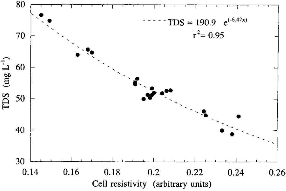
Electrical conductivity depends on the concentration of charged species in the water (Reference Hem, Minear and Keith.Hem, 1982). We convert conductance measured at the stream gauge (recorded as a resistivity) to TDS using the exponential rating curve shown in Figure 6 to obtain a detailed time series of solute concentrations.
Rating curve for TDS and electrical conductivity (measured as a resistivity in the stream-gauge instrumentation). TDS here is the sum of cations (Ca2+, Mg2+, Na+ and K+), anions (HCO3−, SO42−, NO3− and Cl), and silica in the form SiO2, all measured in mg L1.
Snowmelt and air temperature
We measured ablation several times per day using wooden snow stakes at four locations within a roughly 200 m radius of the survey station location, below the terminus of the glacier. The measurements are therefore most relevant to the lower kilometer of the glacier. Stake locations were changed slightly at the time of each measurement to minimize growth of ablation cones. Snow density was measured at only a few locations; we convert the lowering of snow thickness to loss of water equivalent using the mean measured density of 490 kg m3. In addition to the snowmelt measurements, ice ablation was estimated by the emergence from the glacier surface of the drill rods on which the triple reflectors were mounted.
We use the positive degree-day (PDD) approach (e.g. Reference Braithwaite, Olesen. and OerlemansBraithwaite and Olesen, 1989; Reference BraithwaiteBraithwaite, 1995) to densify these measurements temporally and to extend them areally to estimate the snowmelt rate on the entire glacier. The PDD approach relates the ice- or snowmelt in a given period of time (usually a day) to the air temperature, in number of degrees above 0°C, for that period (i.e. melt = γT for T > 0°C and melt = 0 for T > 0°C). To calibrate the factor, γ, in the PDD calculation, we use the temperature measured in the stream-gauge data-logger box at 15 min intervals. We plot the temporal integral of the box-temperature time series, using the time unit of days, and the cumulative snowmelt water equivalent for each of our ablation stakes, as functions of time (Fig. 7). The model curve, representing the product of a specified γ and the temperature history, can be made to match the snowmelt data well using γ = 3.1 mm d1 °C1 (curve labeled 0). While this is at the low end of the range reported by Reference BraithwaiteBraithwaite (1995) in his summary of existing snowmelt datasets, this can be explained by the fact that the temperature of the exposed gray box is typically higher during the daytime than the local air temperature. (A γ of 4.3 mm d1 °C1 obtained from a short air-temperature time series was not used, because the data-logger box temperature has the longer time series.) The best constant-γ model of snowmelt begins to underestimate the snowmelt rate late in the study. This is likely due to a reduction in the albedo of snowpack with age, which should therefore increase γ toward that of pure ice (roughly two times greater than for snow; Reference BraithwaiteBraithwaite, 1995). We illustrate this effect with simulations in which γ is allowed to rise linearly through the study period at a specified rate (curves labeled 2, 4 and 6 in Fig. 7). As snow over the glacier probably did not ripen to the extent seen in our ablation-stake array, we use a constant γ = 3.1 mm d1 °C1. Ignoring this effect will result in a conservative estimate of the snowmelt input to the glacier.
Calibration of snowmelt against air-temperature time series to constrain the PDD factor, γ. Spot measurements of snow elevation at four locations are converted to loss of water equivalent using a nominal snow density of 490 kg m−3. Continuous lines represent integrals of the melt through time, calculated from an temperature multiplied by the PDD factor that best fits the rate of snowmelt, here 3.1 mm d1 °C1. Maturation of the snow accounts for growing rate of melt through time, and is modeled here with linear growth of the PDD factor at rates of 0–6 per week (labeled on the curves).

Results
Our 16 days of observation at Bench Glacier can be broken into four distinct periods (Fig. 8). Light snow fell on the first 3 days; consequently water discharge was low and not marked by diurnal oscillations, and total solute concentrations were high. A period of diurnally varying discharge and solute concentration ensued under clear skies starting on 15 June. Ice-surface velocity averaged nearly 0.1 m d1, although, as discussed below, this too was marked by diurnal oscillations. During 22–24 June the diurnal pattern of discharge broke down despite continued clear weather, the ice-surface velocity nearly doubled, and suspended-sediment concentration rose dramatically to a peak late on 24 June. This period of high ice velocity, high discharge and high suspended-sediment flux ended with a rapid increase in water discharge late on 24 June; thereafter, the ice velocity returned to pre-22 June behavior but with a lower mean and lower diurnal variability, and solute concentrations no longer varied diurnally. We consider the occurrences on 22–24 June to be a spring speed-up and flood event, although its effects clearly continue for the remaining 3 days of observations. The chief characteristics of this event are (i) a loss or decrease in diurnal discharge oscillations, (ii) an increase in sliding velocity at our measurement sites, (iii) high suspended-sediment concentration, particularly at the end of the event and during its culminating flood, and (iv) sustained high solute concentrations after the flood event. Below, we discuss the pre-event conditions, the event, and conditions after the event in turn.
Summary of Bench Glacier time series. (a) Displacement record for two reflectors over the 10 days of the electronic distance meter (RDM) record. Scales for the two targets are identical. Error bars denote instrumental standard deviations (lσ) reported by the EDM. Although upper triple reflector (open squares) yielded much larger errors associated with almost double the distance to the reflector, the correspondence between the two records indicates similar three-part history of motion. Numbers indicate mean daily speed at lower target, derived from slopes of linear fits through the displacement history. (b) Water discharge and ice-surface velocity. The latter record is derived from modeling short segments of the displacement time series (Fig. 9). The three periods display distinctly different behaviors. In both the pre- and post-speed-up segments, the speed varies strongly each day, but achieves the same minimum, presumably associated with internal deformation. Speed-up is associated with loss if the strong variation, and is pinned at roughly the highest pre-speed-up velocity. The ̰20% reduction in the post-speed-up velocity is associated with lowering of the maximum speed. Arrows show timing of the following observations: a, high flow destroys the cable support system for tethered fish at gauging station; b, numerous ice chunks, up to 0.5 m in diameter, appear in the stream; c, dirty water observed emerging from small crevasses on the glacier surface near the terminus. (c) Concentrations of suspended sediment and TDS. (d) Chemical and suspended-sediment fluxes from Bench Glacier.
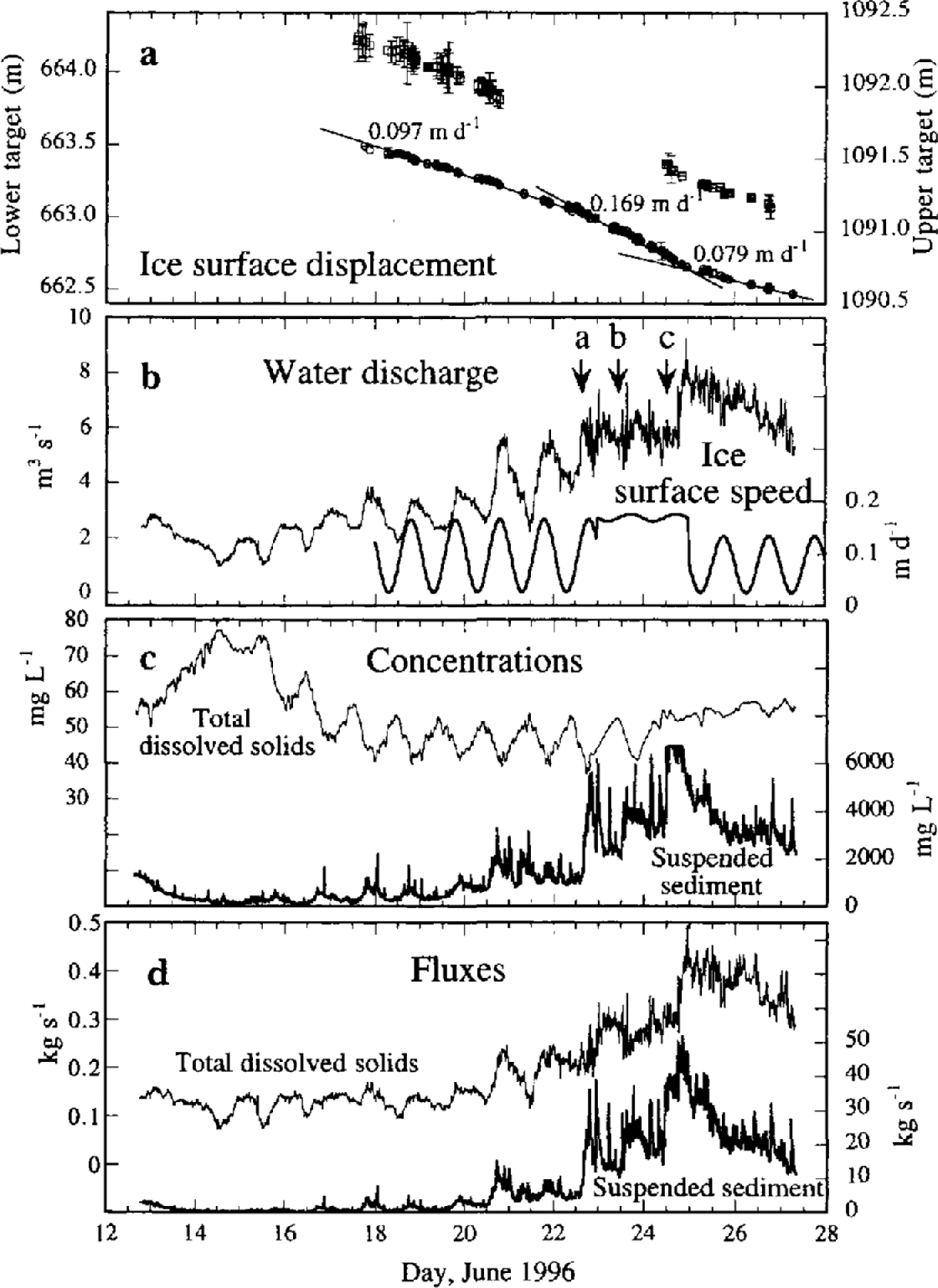
During the clear weather of 15–22 June, the water discharge (Fig. 8b) settled into a diurnally varying pattern. The amplitude of these discharge swings grew through this period, from 1.5 to 3.5 m3 s1, while the mean daily discharge grew from 1.8 to 4.8 m3 s−1. The average ice-surface speed during this time was 97 mm d−1, but on closer inspection, strong diurnal variations can be seen (Fig. 9).
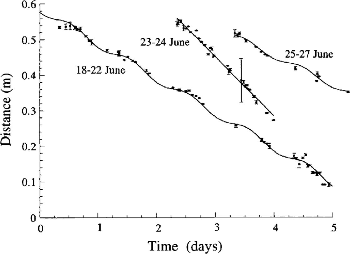
Details of displacement records for lower target on ice, fit by the integral of a sinusoidally varying velocity history (see text). Error bars denote instrumental standard deviations (1σ) reported by the EDM. The three segments correspond to the three straight-line segments shown in Figure 8a. For each segment, midnight corresponds to major tick marks. Ice-surface speeds shown in Figure 8b are the derivatives of the curves shown here. Although night-time measurements are sparse, the high amplitude variation in slope requires significant variations in speed in the 18–22 June and 25–27 June segments.
Pre-event conditions
Sliding speeds
The records of distances to the two targets are shown in Figure 8a. As the errors associated with the lower target are considerably smaller than those of the upper target, we focus here on this lower displacement record. We analyzed the data in three distinct segments (Fig. 9). The curve fits are based upon the assumption that the surface speed is composed of a steady component associated with internal deformation, U d, and a diurnally fluctuating component associated with sliding. Although one could choose any of many periodic functions for the oscillating component, we have chosen to use a simple sinusoidal function, the primary goal being to assess the amplitude and the phase of the fluctuations:
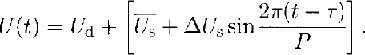
The displacement record is simply the integral of the velocity, or
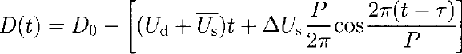
where D 0 is the initial distance to the target, ![]() is the mean sliding speed, ΔU s is the half-amplitude of the speed fluctuation, P is the period of the fluctuation (here set to 1 day) and τ is the lag relative to midnight (t = 0). Inspection of Figure 9 shows that a sinusoidal fluctuation in velocity captures the essence of the displacement records for each of the three data segments. In each case, we fit for all parameters of the velocity history except for the period. The combined modeled velocity record is shown in Figure 8b. Crudely, we interpret the low minimum velocity to be that associated with internal deformation; this is attained in both pre- and post-speed-up intervals.
is the mean sliding speed, ΔU s is the half-amplitude of the speed fluctuation, P is the period of the fluctuation (here set to 1 day) and τ is the lag relative to midnight (t = 0). Inspection of Figure 9 shows that a sinusoidal fluctuation in velocity captures the essence of the displacement records for each of the three data segments. In each case, we fit for all parameters of the velocity history except for the period. The combined modeled velocity record is shown in Figure 8b. Crudely, we interpret the low minimum velocity to be that associated with internal deformation; this is attained in both pre- and post-speed-up intervals.
As shown in Figure 8b, the speed fluctuations are well correlated with discharge fluctuations, as expected if sliding rates are indeed modulated by some aspect of the hydrologic system. Here the speed reaches a maximum in concert with the discharge maximum at ~1800–1900 h. We have less confidence in the correspondence of the minima, as the early-morning surface speeds are less well constrained.
The spring event
On 22 June and for the next 2 days, the amplitudes of the discharge and sliding-speed diurnal variations decreased while the means increased to a level comparable to the peak values of the previous days. This gives the appearance of an abrupt loss of oscillatory character in these parameters (Fig. 8b). This period of sustained high discharge and ice velocity was accompanied by large increases in the concentration of suspended sediment (Fig. 8c). The sediment shows peaks roughly centered around 1800 h, a time when water discharge from snowmelt should reach a maximum for the day. Solute concentrations remain oscillatory through this period, with no change in amplitude or mean.
The sediment discharge is plotted in Figure 8d. The sediment removed in suspension over the course of the large peak in sediment discharge is greater than the total suspended-sediment flux in the 10 days prior to this event. The maximum discharge of 40 kg s−1 is large for the scale of the glacier, corresponding to 48 mm a−1 of lowering of the glacier bed if sustained for an entire year.
We have anecdotal evidence of substantial subglacial hydrologie reorganization during this period. On 23 June we noticed a number of large (up to 0.5 m diameter) ice chunks in the outlet stream. As not even minor collapse of ice at the outlet portal was observed, these chunks must have been derived subglacially. At about noon on 24 June, one of us (R.S.A.) traversing the glacier between the lower triple reflector and the ice margin heard numerous sounds coming from within the ice, and encountered a turbid stream flowing on the ice as it emerged from a thin crevasse. Presumably, high water pressures within the glacier forced this turbid water to the surface from the bed.
The spring event terminated late on 24 June with a step increase in the discharge of ~3 m3s−1, or 50%, in 4 hours, accompanied by the highest observed suspended-sediment concentrations. As our turbidity sensor was saturated during this period, the sediment concentrations and fluxes in Figure 8 represent minimum estimates.
Post-event conditions
The period after the discharge peak on 24 June differs in character from both the event and the pre-event period (Fig. 8). Discharge fell slowly after its sharp culmination, with no evidence of diurnal oscillation. Ice-surface speed, however, returned abruptly to a lower average rate. Sediment concentrations fell dramatically. The one record that does not show a relaxation following the heightened activity of the spring event is that of solute concentrations. The steady diurnal oscillations of TDS (Fig. 8c), maintained before and during the event, disappear on 24 June, to be replaced with a period of steady, high concentrations. Because the TDS remains high after the termination of the event, the solute flux remains high after 24 June, instead of falling as the suspended-sediment flux docs (Fig. 8d).
It is likely that the channel cross-section at the stream-gauge site varied through the flood event. The need to reset our discharge rating curve because of apparent aggradation on 26 June suggests that a wave of coarse sediment may have reached our gauging site at that time, lagging behind the documented pulse of suspended sediment on 24–25 June. Reference WarburtonWarburton (1992) observed a wave of aggradation that propagated down the Bas Glacier d’Arolla (Swiss Alps) outlet stream following scour in a large flood. It seems likely that the aggradation we infer on 26 June was of this nature, although there is no indication of scour during the flood, either at our gauging site or upstream.
Discussion
We believe that the speed-up and flood event of 22–24 June represents the build-up of subglacial water pressure near the terminus in a dominantly distributed flow system, and subsequent release of pressure and reduction in sliding speed due to extension or formation of one or more subglacial conduits. High sliding velocity and high water discharge are strongly correlated both before and during the event. If sliding velocity is modulated by basal water pressures, then this correspondence suggests that the water discharge can be used as a proxy for subglacial water pressures near the terminus. The observation of turbid water spilling onto the glacier surface on 24 June indicates at least locally high subglacial water pressures during the even. The suspended-sediment flux associated with this event likely represents evacuation of stored sediment by turbulent water flow accessing new parts of the bed (Reference Willis, Richards. and Sharp.Willis and others, 1996), suggesting either that new conduits formed or that existing conduits migrated. The large ice chunks spewed out during the event support the former interpretation.
The important question is what triggered this transition in the subglacial drainage system. A storm did not precipitate the event; although light rain fell a few hours before the culminating flood, none fell in the 9 days before the event. We examine below the water balance for the glacier during this time interval in an attempt to quantify the timing and magnitude of changes in storage of water subglacially.
Water inputs to the glacier from melt
Given the locally calibrated relation between air temperature and snowmelt water equivalent, we generate a time series of water inputs to the glacier. The calculation is based on an assumption that there was no sublimation or loss of snow or ice mass by any process other than surface melting, and that the only source of liquid water was melt due to incoming solar radiation. As the positive degree-day factor γ is about two times greater for ice than snow (Reference BraithwaiteBraithwaite, 1995), we must also constrain the evolution of the fraction of the glacier that was bare ice through the short period of our study. These constraints come from two observations of the glacier surface from the air, on our incoming (0% exposed ice) and outgoing (30% exposed ice) flights. We assume a linear variation of the exposed ice fraction, f ice, from 0.0 to 0.3 over the 16 day study period. We also calculate the snowmelt from the non-glacierized portion (28%) of the catchment. The fraction of this area that is exposed rock on the valley walls, f rock, increased from roughly 30% to 80% over the study period; we assume this too increases linearly. Although, as discussed above, we are aware that the albedo of snow declines considerably as it ripens, incorporation of this effect is unwarranted given the other errors in our data. We seek a conservative estimate of snowmelt water equivalent from the basin.
The resulting summed snow- and ice-melt water inputs, Q in(t), to the glacial system are therefore determined through

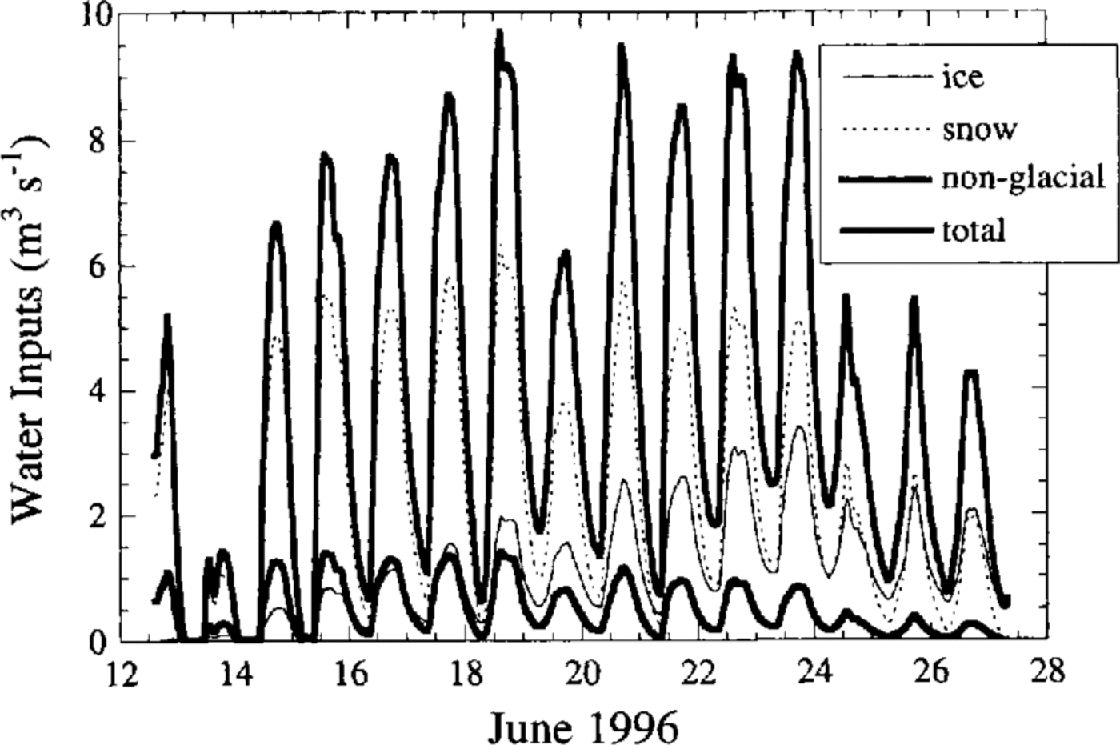
where γ is the PDD factor (here we take γsnow = 3.1 mm d1 °C−1 and γice = 6.2 mm d−1 °C−1), A b is the total area of the basin, and A g is the area of the glacier. All temperatures are mean temperatures of those portions of the catchment, calculated using the data-logger box temperature and an assumed lapse rate of 6.5°C km1. The first term corresponds to melt production from the glacier, the second to melt production from the non-glacierized part of the catchment. The result of this calculation is plotted in Figure 10. The integrated melt varies by many-fold daily, with a range over the study period of essentially 0 (freezing nights) to ~10 m3 s−1. While the contributions of water from snowmelt show a general decline, those from ice melt generally increase through the study period. The non-glacierized part of the catchment contributes minimally (>1 m3 s−1) and declines through time as snowmelt exposes bare rock. Given the lack of significant rain over most of the period (until 24 June), the solar-radiation-driven melt shown in Figure 10 represents the primary source of water to the glacier. Cloudiness on 19 June lowered the melt maximum, while on 24 June a storm system began delivering light rain, lowering significantly the expected melt rate.
Calculated meltwater production using Equation (6). The melt production includes contributions from snowmelt in upper catchment and from ice melt in lower catchment, and snowmelt from the non-glacierized part of the catchment. Proportion of glacier with exposed ice varies linearly from 0 to 30%, while proportion of non-glacierized catchment with bare rock varies from 30% to 80% over the measurement interval. The fraction of the flow attributable to ice melt grows through time, while that associated with snowmelt on both glacier and non-glacier parts of the catchment declines. Maximum contribution from non-glacierized catchment is roughly 10%.
Water inputs, outputs and changes in storage
The calculated snow- and ice-melt inputs and the measured outputs are plotted together in Figure 11. Although the input side of the water balance is only roughly constrained, the order of magnitude and timing of melt must be correct. Several features of the curves are important. First, the amplitude of the variations in the melt inputs is significantly greater than that of the discharge from the glacier. Peak melt production approaches 10 m3 s1, while peak discharge before the flood event is no more than about 6 m3 s−1. Conditions on 12–14 June were cold and snowy, and melt production fell to zero overnight, while discharge declined. Second, while there is always a lag between melt input and stream discharge, this lag decreases steadily before and through the event from 6 hours to 2.75 hours (Fig. 11b), possibly reflecting an increase in efficiency of the subglacial hydrologic system. The nearly 10 hour lag at the culmination of the event on 24 June shows that this flood was unrelated to diurnal melt variations, and suggests that instead it represents the establishment of a different drainage route. Third, before the event, the mean daily rate of input to the system is consistently greater than the mean daily discharge from the system. In the clear-weather pre-event period (15–22 June), inputs average 4.5 m3 s1, while daily discharge averages 2.9 m3 s−1. This relationship changes abruptly after 22 June. For 2 days, inputs and outputs were roughly equivalent, and starting 24 June, outputs exceeded inputs.
(a) Water inputs and outputs from Bench Glacier through the 16 day observation period. Rain measured in Valdez, 25 km west, correlates with changes in melt, but is insufficient to alter greatly the net inputs to the glacier. Until 24 June, mean daily runoff is less than mean daily melt production, implying net englacial storage. (b) Lag between maximum calculated meltwater production and measured peak discharge. The time-scale of the lag declines from 6 hours to 2 hours by the time of the flood on 24 June. (c) Cumulative melt production and runoff through the period of observations. The difference between these curves is subglacial storage of water, here normalized to the 9 km2 area of the glacier.
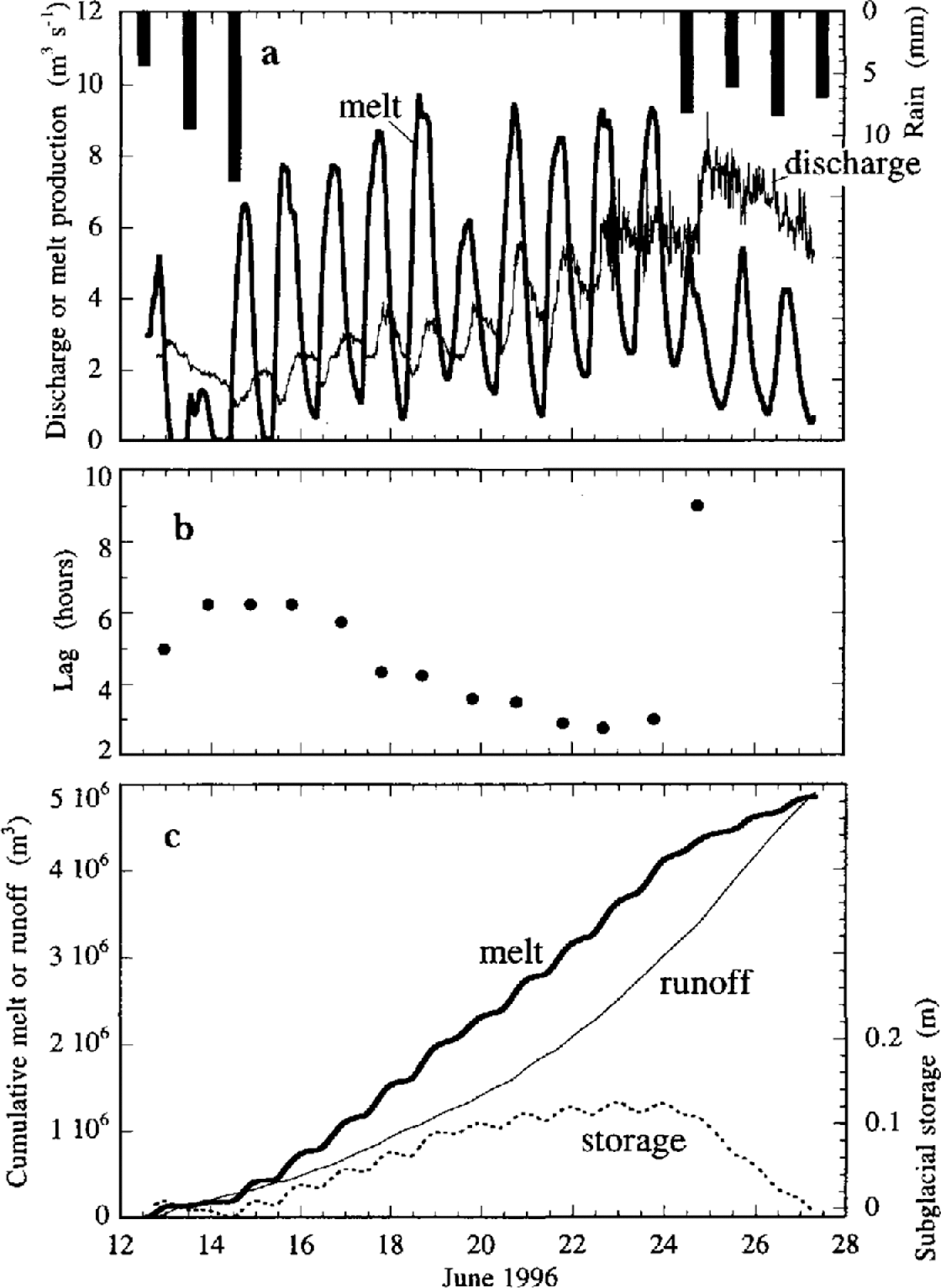
The water balance is further illustrated in Figure 11c, in which we plot the cumulative snow- and ice-melt inputs, the cumulative water outputs and the implied history of storage. The storage is calculated as (inputs – outputs) /area of glacier, and is therefore in units of m w.e. within the glacier, and includes water stored within snow and firn. We recognize that this calculation compounds the errors in our discharge measurements and melt calculations. We present the results because the pattern we obtained, without manipulation, displays interesting parallels with other, more robust observations. The pre-event period is characterized by inputs in excess of outputs, and accumulation of water in storage. The calculated storage stabilized at a value of roughly 0.13 m on 22 June, the time when the diurnal discharge variations diminished. Interestingly, it appears that the cumulative discharge in the flood was sufficient to drain a significant fraction of the water stored within the glacier from the early melt season. Recalling that the snowmelt calculations led to conservative estimates, the apparent drawdown of storage to zero at the end of the observation period is fortuitous. Reference Iken, Röthlisberger, Flotron. and Haeberli.Iken and others (1983) observed surface uplifts, attributed to water storage, of up to 0.2 m over periods of a few days at Unteraargletscher, in keeping with the magnitude of water storage calculated here. More careful estimation of water storage within a glacier could lead to greater insight into the connections between sliding and storage; this would be best achieved with better characterization of melt, inputs over the entire glacier.
The decline in lag between melt production and runoff peaks is indicative of a drainage system that is increasingly efficient at delivering water to the stream. Certainly, part of this efficiency gain comes from increasing areas of bare ice that rapidly transmit melt into crevasses and moulins. However, the greater than two-fold drop in lag time seen over the course of this study is much greater than the ~30% increase in exposed ice surface on the glacier. Some of this increased efficiency must derive from greater connectivity of cavities in the days preceding the flood event. The growth in peak discharge in the pre-event period, despite relatively constant inputs, also speaks to more efficient delivery of water through the subglacial system. Despite the increasing efficiency of the subglacial hydrologic system, the calculated storage continued to increase. It is this backing-up of water in the system that presumably leads to increased basal water pressures and sustained sliding.
The mismatch between discharge outputs of water and meltwater inputs is just balanced at the beginning of the speed-up event on 22 June. The storage had increased slowly to slightly more than 0.1 m, averaged over the entire glacier bed, at the beginning of the speed-up, and then “stabilized” over the next 2 days. During this period of near-parity between discharge and meltwater inputs, ice chunks in the outlet stream and sounds emitting from the glacier suggest to us that significant rearrangement, presumably enlargement, of subglacial conduits was occurring. The ultimate flood on 24 June, during a period of declining meltwater inputs, appears to represent the final push in establishing a subglacial drainage system capable of draining the accumulated meltwater. Its timing is unrelated to diurnal meltwater inputs, and the discharge thereafter is in excess of inputs.
Runoff chemistry
Before 24 June, the concentrations of dissolved solutes in the runoff varied inversely with discharge each day (Figs 8c and 12). These diurnal variations are normal in glaciers, and arise from variations in the pathways by which water reaches the outlet (Reference CollinsCollins, 1979; Reference Tranter and Raiswell.Tranter and Raiswell, 1991; Reference Tranter, Brown., Raiswell., Sharp. and Gurnell.Tranter and others, 1993), and variations in the contact time of water with subglacial sediments (Reference CollinsCollins, 1995; Reference Brown, Tranter. and Sharp.Brown and others, 1996a). Low solute concentrations are associated with high fluxes of dilute supraglacial meltwaters that have travelled rapidly through the glacier with minimal interaction with the bed, while high solute concentrations are found in water that has had intimate contact with the glacier bed.
The relationship between solute concentrations (as measured by TDS calculated from conductivity) and discharge in the Bench River can be broken into three distinct behaviors. The pre-event period (up to 22 June) is marked by a strong inverse relationship between TDS and discharge. During the speed-up event (22–24 June), TDS and discharge are uncorrelated. After the flood on 24 June, in the post-event period, solute concentrations are independent of discharge.
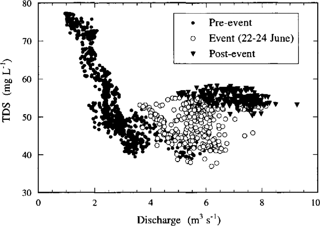
The simple inverse relationship between TDS and discharge broke down during the speed-up and flood event. Diurnal oscillations in TDS continued at the same amplitude through the speed-up event, despite a reduction in the amplitude of discharge variations; the TDS oscillations disappear in the flood culminating the spring event, and remain suppressed for the remaining 3 days of observation (Fig. 8c). These changes yield three classes of behavior on a plot of TDS concentration as a function of discharge (Fig. 12). Before the speed-up and flood event, concentrations vary inversely with discharge. On 22–24 June, discharge variations declined, but TDS oscillations continued, resulting in a lack of correlation between these parameters. The post-event (post-24 June flood) data plot as a horizontal band (Fig. 12), showing that TDS is independent of discharge during this period. During both the flood event and the post-event period, concentrations are higher than would have been predicted by the concentration–discharge relationship of the pre-event period.
The persistence of diurnal oscillations in chemistry during 22–24 June, while the amplitude of variations in the discharge is diminished, implies that during this period distinct pathways exist transmitting low-solute water and high-solute water to the outlet stream, and that the relative contributions from these pathways varied diurnally (Fig. 8). The average discharge during this 2 day event was higher than during the preceding 10 days. Normally, increases in discharge are accompanied by a decrease in TDS. During 22–24 June, however, TDS was in the same range as in the preceding days (Fig. 12), implying either a greater flux or higher TDS from the high-solute source during this period. After the 24 June flood, the combination of high solute concentrations and loss of diurnal fluctuations suggests that the discharge in the post-event period is dominated by water that had been stored subglacially, and that the diurnal flushes of dilute meltwater are completely overwhelmed by water from this source.
Several features of the water chemistry, detailed in Figure 13, are of interest. Although the TDS after 24 June is similar to that during the low-flow period of the days preceding the flood, the speciation is different. In particular, sodium is much more concentrated, pH is higher and P CO2 with which the water is in equilibrium is lower in the runoff after 24 June. The trend is less clear, but also suggestive of higher concentrations in the post-flood days, for potassium, silica and nitrate. None of these trends are correlated with the suspended-sediment pulse, which peaked before the solute concentrations in bulk runoff shifted (Fig. 8), and therefore “post-mixing” reactions (Reference Brown, Sharp., Tranter., Gurnell. and Nicnow.Brown and others, 1994; Reference Sharp, Brown., Tranter., Willis. and Hubbard.Sharp and others, 1995) between dilute waters from surficial melt and sediment-laden waters at the bed are not a likely-cause of the change in concentrations.
Composition of Bench River water through time. Gray curves show TDS concentrations calculated from EC measurements (leak on right side), while connected points show measured composition of water samples (scales on left sides of plots).
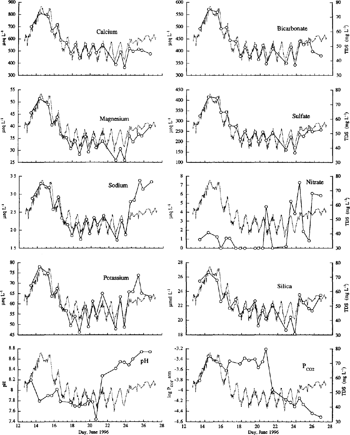
One of the most important weathering reactions responsible for the chemistry of runoff from glaciers, regardless of the bedrock, is dissolution of trace quantities of carbonate minerals (Reference RaiswellRaiswell, 1984; Reference Mast, Drever. and Baron.Mast and others, 1990; Reference Tranter, Brown., Raiswell., Sharp. and Gurnell.Tranter and others, 1993; Reference Brown, Sharp. and Tranter.Brown and others, 1996b; Reference Anderson, Drever. and Humphrey.Anderson and others, 1997; Reference Blum, Gazis., Jacobson. and Chamberlain.Blum and others, 1998), which increases the pH and releases calcium, magnesium and bicarbonate to the water. This reaction can be coupled to iron sulfide (e.g. pyrite) oxidation (Reference Tranter, Mills., Raiswell. and MilesTranter and others, 1989, 1993), which produces sulfate and hydrogen ions capable of driving further carbonate dissolution. The effects of these processes can be seen in the Bench Glacier runoff in the high calcium, magnesium, bicarbonate and sulfate concentrations. If anything, these species appear to be present in slightly lower concentrations following the 24 June flood, suggesting that the products of these reactions are being diluted. High pH and low P CO2 seen after 24 June are the characteristics one expects to see in waters that have evolved in a system closed to atmospheric CO2 (Reference RaiswellRaiswell, 1984).
The enhanced sodium, potassium and silica concentrations after 24 June in the Bench River (Fig. 13) are consistent with a source from weathering of aluminosilicate minerals. These reactions are most likely to take place where water and sediments are in contact for long periods of time, as the kinetics of silicate-weathering reactions are slow (Reference Lasaga, Soler., Ganor., Burch. and Nagy.Lasaga and others, 1994). Reference TranterTranter and others (1997) associated high silica, base-cation, bicarbonate and sulfate concentrations with the subglacial distributed flow system, because that is the only subglacial environment where there is sufficient contact time between sediments and water for acquisition of solutes in concentrations high enough to produce an observable shift in the runoff. We similarly infer that the high solute concentrations, and in particular the high cations and silica, and low P CO2 of the post-flood period are indicative of the runoff being overwhelmed by water draining the distributed drainage system.
Finally, it is worth noting the nitrate in the runoff. Although the trend is not unequivocal, there is a tendency for nitrate to be present in measurable quantities (up to 7μeq L−1) following the 24 June flood, while it is either undetected or present in very low concentrations before this flood (Fig. 13). Reference TranterTranter and others (1997) noted mean nitrate concentrations of 27 μeq L−1 in boreholes that appeared not to be connected to subglacial conduits, i.e. in waters from the distributed flow system at Haut Glacier d’Arolla, Switzerland. They suggested that the nitrate came from preferential elution of nitrate from the snowpack during early snowmelt, and that its presence demonstrates storage of water subglacially for periods on the order of months. The high nitrate in the runoff at Bench Glacier during a time when we infer that stored meltwaters dominate the discharge is in keeping with this interpretation.
Summary
Drawing on evidence from the pattern of discharge, glacier surface velocities, sediment and solute concentrations, and physical observations, we can now build the following conceptual model of the spring event we observed at Bench Glacier. The sunny weather of 15–22 June produced meltwater at a rate greater than the subglacial drainage system could transmit. Consequently, water storage within the glacier increased. This storage may have been in any part of the glacier: within the snowpack, within englacial conduits or at the glacier bed. We believe that subglacial storage was the most important. Although either englacial or sub-glacial storage could produce the high water pressures we infer from the enhanced sliding velocities on 22–24 June, only release of subglacially stored water can explain the shift to high TDS and altered speciation in the runoff after the speed-up event. During the period of sustained high sliding speeds, the glacier seemed to be in a quasi-equilibrium with respect to water balance. The calculated meltwater production was approximately equal to the discharge over this interval, although peak meltwater production each day exceeded the discharge at any time. Physical evidence in the form of high sediment concentration and large ice chunks appearing in the outlet stream suggests that new subglacial flow paths, which would provide routes for high-solute subglacial water to drain, were formed forcefully during this interval. Diurnal solute concentration variations remained intact, showing that some conduits capable of rapid transmission of recent meltwater through the glacier persisted through this period; however, increased solute flux during this time shows that a reservoir of high-solute water was being tapped. The culminating flood on 24 June released a huge pulse of suspended sediment and water, and put an end to the period of high sliding velocity. We infer that high subglacial pressures were relieved by this flood. However, in many ways the system does not return to pre-event character. The mean sliding speed was lower, reflecting an increase in the mean effective stress at the bed. The chemistry of the runoff was altered by this event to a composition similar to distributed-system subglacial waters sampled elsewhere (e.g. Reference Tranter, Brown., Hodson. and Gurnell.Tranter and others, 1996), normally a dominant component of the runoff only during periods of low flow. For the remaining 3 days of observation, the discharge appears to be dominantly draining water that had been stored subglacially. Presumably, had we continued our measurements longer we would have seen the re-establishment of diurnal oscillations in the solute concentrations and discharge as the hydrologic system regained a balance.
Conclusions
Bench Glacier displayed a transient response in sliding, and in the chemistry and physical sediment delivered through the subglacial system, reflective of the reorganization of the hydrologic system at the bed. This event appeared to be caused by a period of inputs of meltwater in excess of the capacity of the subglacial drainage system. Repercussions in the discharge record, suspended-sediment concentrations and solute concentrations lasted for several days after the peak flood event, which we believe reflects the drawdown of subglacial water storage. Because Bench Glacier docs not have a complicated drainage area, and appears not to have a complex bed geometry, this event must be driven by internal responses that are common to all glaciers, and not unique to particular settings. The causes of such episodes may be more readily understood in small, simple glaciers such as Bench Glacier.
Acknowledgements
We wish to thank K. Goscinski for aid in the fieldwork, and S. Boese at University of Wyoming and R. Franks in the Marine Analytical Laboratory at the University of California, Santa Cruz, for help with chemical analyses. We thank K. C. MacGregor and L. Perg for commenting on an earlier draft of the manuscript, and M. Tranter and an anonymous reviewer for their careful critiques. This study was funded in part through a U.S. National Science Foundation (NSF) Earth Sciences post-doctoral fellowship (EAR-9404465) to S.P.A., and through an NSF Presidential Young Investigator award to R.S.A. This is contribution No. 386 from the Institute of Tectonics.


