


Media summary: Coupled contagion model explains how anti-vaccine sentiment, treated as a ‘cultural pathogen’, can promote spread of infectious disease.
Introduction
Models of cultural evolution examine the dynamics of cultural traits in populations in a manner similar to that of population-genetics studies of the dynamics of genetic variants (Cavalli-Sforza & Feldman, Reference Cavalli-Sforza and Feldman1981; Boyd & Richerson, Reference Boyd and Richerson1985; Mesoudi, Whiten, & Laland, Reference Mesoudi, Whiten and Laland2006). Such models make use of analogous but distinct mechanisms of transmission for cultural and biological characters, as well as analogues of population-genetic processes such as mutation and natural selection.
When a culturally transmitted trait affects the health, reproduction or survival of individuals who carry it, the dynamics of the trait can influence the dynamics of characteristics that are transmitted genetically (Feldman & Laland, Reference Feldman and Laland1996; Ross & Richerson, Reference Ross and Richerson2014; Creanza et al., Reference Creanza, Kolodny and Feldman2017) or by other biological mechanisms – such as by the spread of biological pathogens (Tanaka et al., Reference Tanaka, Kumm and Feldman2002; Epstein et al., Reference Epstein, Parker, Cummings and Hammond2008; Salathé & Bonhoeffer, Reference Salathé and Bonhoeffer2008; Funk et al., Reference Funk, Gilad, Watkins and Jansen2009, Reference Funk, Salathé and Jansen2010; Perra et al., Reference Perra, Balcan, Gonçalves and Vespignani2011; Bauch & Galvani, Reference Bauch and Galvani2013; Wang et al., Reference Wang, Andrews, Wu, Wang and Bauch2015). In considering a culturally transmitted trait that has deleterious health effects, we can focus on the concept of a cultural pathogen: a culturally transmitted trait whose presence in an individual negatively affects a health-related trait.
In the narrowest sense, we define a cultural pathogen as having a detrimental impact on a specific health-related trait, leaving its impact on other health-related traits unspecified. For example, the concept of a cultural pathogen might be applied to a practice such as ritual eating of the dead in the Fore people of Papua New Guinea, which contributed to transmission of the prion disease kuru (Feldman & Cavalli-Sforza, Reference Feldman and Cavalli-Sforza1976; Durham, Reference Durham1982; Lindenbaum, Reference Lindenbaum2008; Whitfield, Pako, Collinge, & Alpers, Reference Whitfield, Pako, Collinge and Alpers2017). The class of cultural pathogens includes premodern medical treatments such as bloodletting, which generally exacerbated rather than alleviated disease conditions and whose continued use was a consequence of cultural transmission in the medical profession (DePalma, Hayes, & Zacharski, Reference DePalma, Hayes and Zacharski2007; Miton, Claidière, & Mercier, Reference Miton, Claidière and Mercier2015). Persistent folk remedies that have no discernible benefit against diseases they are designed to treat and even cause significant harm – such as the use of harsh chemicals to treat cutaneous leishmaniasis (Ramdas, Reference Ramdas2012) and the use of elements such as arsenic, lead and mercury in herbal preparations in traditional Indian medicine (Ernst, Reference Ernst2002; Saper et al., Reference Saper, Phillips, Sehgal, Khouri, Davis, Paquin and Kales2008) – are also cultural pathogens (Tanaka, Kendal, & Laland, Reference Tanaka, Kendal and Laland2009). Note that our sense of a cultural pathogen is similar to treatments of maladaptive cultural traits in evolutionary models (e.g. Cavalli-Sforza & Feldman, Reference Cavalli-Sforza and Feldman1981; Boyd & Richerson, Reference Boyd and Richerson1985); unlike in these treatments, however, we consider the consequences of the cultural trait not on biological fitness but on a specific aspect of health.
The dynamics of social contagions – contagious ideas, information or sentiments (Bauch & Galvani, Reference Bauch and Galvani2013) – have long been of interest (Goffman & Newill, Reference Goffman and Newill1964), possessing many parallels to the dynamics of biological contagions. Among social contagions, the class represented by cultural pathogens generates coupled social and biological dynamics, as dynamics of the cultural pathogen influence those of the associated health-related trait. Thus, to investigate the dynamics of the health-related trait, it is important to consider the dynamics of the cultural pathogen. A coupled perspective can complicate the dynamics of the health-related trait beyond what would be observed in studying its behaviour without the cultural pathogen (Epstein et al., Reference Epstein, Parker, Cummings and Hammond2008; Funk et al., Reference Funk, Salathé and Jansen2010; Wang et al., Reference Wang, Andrews, Wu, Wang and Bauch2015).
Anti-vaccine sentiment – an individual predisposition to intentionally avoid vaccination against an infectious disease – is a culturally transmitted trait (Dubé, Vivion, & MacDonald, Reference Dubé, Vivion and MacDonald2015) that persists endemically in some populations (Gangarosa et al., Reference Gangarosa, Galazka, Wolfe, Phillips, Miller and Chen1998; Salathé & Khandelwal, Reference Salathé and Khandelwal2011; Mellerson et al., Reference Mellerson, Maxwell, Knighton, Kriss, Seither and Black2018; Morrison, Castro, & Meyers, Reference Morrison, Castro and Meyers2020), often despite significant intervention (e.g. Delamater, Leslie, & Yang, Reference Delamater, Leslie and Yang2017). Assuming that a vaccine provides effective protection against an infectious disease, this anti-vaccine sentiment can be regarded as a cultural pathogen in relation to the disease against which the vaccine protects. Not being vaccinated is a risk factor for disease infection; therefore, irrespective of its effects on other behaviours or health-related traits, a culturally transmitted anti-vaccine sentiment satisfies the condition for being a cultural pathogen in relation to the target infectious disease.
Coupled dynamics of anti-vaccine sentiment (a cultural pathogen) and infection by the infectious agent against which the vaccine protects (a biological pathogen) provide a natural example for investigation of coupled contagions. At the same time, analysis of a coupled contagion model can provide insight into the effects of anti-vaccine sentiment dynamics on infectious disease dynamics. Here, we seek to understand the effects of the dynamics of anti-vaccine sentiment on the dynamics of an infectious disease. We build a model of a culturally transmitted anti-vaccine sentiment that acts as a cultural pathogen influencing infection with the disease targeted by the vaccine. We consider a susceptible–infected–resistant (SIR) compartmental model for disease dynamics, coupling it with a separate SIR model for cultural dynamics of the anti-vaccine sentiment.
Model
Our model concerns two dynamical processes: the spread of an infectious disease and the spread of anti-vaccination sentiment. Disease transmission follows a traditional SIR framework (Kermack & McKendrick, Reference Kermack and McKendrick1932; Hethcote, Reference Hethcote2000) with vaccination. We treat anti-vaccination sentiment as a cultural pathogen: by analogy with the SIR model of a transmissible biological pathogen, we model anti-vaccine sentiment as a contagion that can be transmitted to a susceptible individual upon interaction with an ‘infected’ anti-vaccine individual. Transmission of sentiment is analogous to that of an infectious agent and follows an SIR framework in which individuals enter the population susceptible to a contagion and can become sentiment-‘infected’ by interacting with sentiment-infected individuals. Sentiment-infected individuals can ‘recover’ and become pro-vaccine. Pro-vaccine individuals are immune to anti-vaccine sentiment upon further exposure. We treat sentiment-susceptible individuals as undecided about vaccines, and they can become pro-vaccine without having been previously anti-vaccine; this transition represents ‘vaccination’ against the cultural pathogen. Only pro-vaccine individuals can become vaccinated against the disease; this restriction is the mechanism by which the sentiment can facilitate disease spread.
The modelling approach encapsulates phenomena observed in the dynamics of anti-vaccine sentiment. To emphasize the link between the social contagion of anti-vaccination sentiment and the biological contagion of the disease, the model considers sentiment transmission by person-to-person communication, such as by social networks (Brunson, Reference Brunson2013) and social media (Salathé & Khandelwal, Reference Salathé and Khandelwal2011; Salathé, Vu, Khandelwal, & Hunter, Reference Salathé, Vu, Khandelwal and Hunter2013); it does not consider adoption of anti-vaccine sentiment through other means (Funk et al., Reference Funk, Salathé and Jansen2010; Dubé et al., Reference Dubé, Vivion and MacDonald2015), such as via individual perception of vaccination and disease risks (Lewis & Speers, Reference Lewis and Speers2003; Smailbegovic, Laing, & Bedford, Reference Smailbegovic, Laing and Bedford2003; Wombwell et al., Reference Wombwell, Fangman, Yoder and Spero2015) or interactions between individual-based and social acquisition modes.
The model also accounts for distinctions observed between anti-vaccine and pro-vaccine sentiment. It treats pro-vaccine transitions as individual decisions without social influence, reflecting results that the complex phenomenon of anti-vaccine sentiment (Dubé et al., Reference Dubé, Vivion and MacDonald2015; Peretti-Watel et al., Reference Peretti-Watel, Larson, Ward, Schulz and Verger2015) behaves more like a contagion than does pro-vaccine sentiment (Salathé et al., Reference Salathé, Vu, Khandelwal and Hunter2013). In this framework, pro-vaccine sentiment acts as a cultural inoculation against transmissible anti-vaccine sentiment (McGuire & Papageorgis, Reference McGuire and Papageorgis1961; Banas & Rains, Reference Banas and Rains2010) rather than as a transmissible sentiment itself.
To encode the dynamics of the coupled biological and cultural pathogens, we consider a coupled pair of SIR systems, one for disease and one for anti-vaccine sentiment. The population has nine compartments, each corresponding to a pair of classes from the two systems. The disease classes are susceptible (S), infected (I) and resistant (R). The resistant class includes vaccinated individuals. Sentiment classes are undecided (U), anti-vaccine (A) and pro-vaccine (P).
An SIR model with vaccination, vital dynamics (births and deaths), and constant population size S + I + R = 1 has four parameters: birth rate b, disease transmission rate r for S → I transitions, disease recovery rate g for I → R transitions, and vaccination rate v for S → R transitions. To maintain a constant population size, we make the standard assumption that birth and death rates are equal, so that the death rate is also b. The dynamics follow a system of equations involving time derivatives of the compartments (Hethcote, Reference Hethcote2000; Keeling & Rohani, Reference Keeling and Rohani2007):

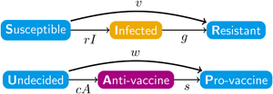
The disease and sentiment components of our model each use the structure of eqn (1). In addition to the disease parameters in eqn (1), our coupled model has three parameters for sentiment dynamics, corresponding to the intercompartmental transition rate parameters r, g and v in the disease model of eqn (1): sentiment transmission rate c for U → A transitions, anti-vaccine-to-pro-vaccine switching rate s for A → P transitions and pro-vaccine decision rate w for U → P transitions. Parameters are summarized in Table 1 and Figure 1a, which displays the two SIR models separately. Unless otherwise stated, we assume that all parameter values are strictly positive.

Diagrams of the model. Compartment variable names follow Table 2 and parameter names follow Table 1. (a) The disease and sentiment susceptible–infected–resistant systems shown separately. (b) The full nine-compartment system. An additional parameter b describes the rate at which individuals are introduced into the population in compartment SU as well as the rate at which individuals are removed from the population in each compartment.

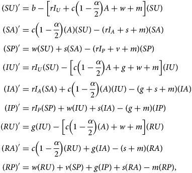
Denoting compartments with two letters, the first for the disease class and the second for the sentiment class (Table 2), dynamics of our model are described by the following system of equations:
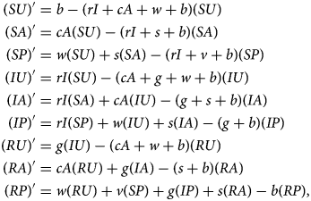
with SU + SA + SP + IU + IA + IP + RU + RA + RP = 1. The two-letter abbreviations represent compartments associated with a specific disease compartment and a specific sentiment compartment. Figure 1b presents a diagram of the full compartmental model described by eqn (2).

The marginal variables S, I, R, U, A and P, representing the disease-susceptible, disease-infected, disease-recovered, vaccine-undecided, anti-vaccine and pro-vaccine classes, respectively, are defined by summing over the associated compartments:

Summing over disease classes and writing eqn (2) in terms of U, A and P yields the SIR model in those variables (eqn 18 in Appendix A – Supplementary Information). We call this system the ‘sentiment subsystem’. Summing over sentiment classes in an analogous way yields the ‘disease subsystem’ (eqn 19 in Appendix A). This system in terms of S, I, and R is close to the standard SIR model (eqn 1), with the only difference being that the vaccination rate v is multiplied by a quantity p = (SP)/S, the fraction of S individuals that are pro-vaccine and therefore the only individuals that can be vaccinated against the disease. This modification is the source of the coupling between the disease and sentiment subsystems, as the sentiment state affects a transition in the disease state through this modification.
The most important quantity in a standard SIR model is the basic reproduction number R 0 (Hethcote, Reference Hethcote2000; Keeling & Rohani, Reference Keeling and Rohani2007), which determines the equilibrium behaviour of the model. For eqn (1), this quantity is R 0 = r/(g + b). For our model (eqn 2), we have two analogous quantities, one for the disease subsystem (R 0) and one for the sentiment subsystem (C 0):


The quantity R 0 (eqn 4) represents the expected number of infected individuals produced by a single disease case, assuming the rest of the population is susceptible to the disease (S ≈ 1). The quantity C 0 (eqn 5) represents the expected number of anti-vaccine individuals produced by a single individual with this sentiment, assuming that the rest of the population is undecided (U ≈ 1).
These quantities reflect the ability of each contagion to be transmitted, and they play important roles in determining equilibrium behaviour. If R 0 or C 0 exceeds 1, then transmission outpaces recovery for the associated contagion. If R 0 or C 0 is even larger, then transmission might also outpace the effects of vaccination and pro-vaccine decisions. It is only if this additional condition is met that the contagion can maintain itself in the population.
Results
Equilibria
We first analyse the equilibrium states. Approach to equilibrium is one possible outcome of the long-term behaviour of a dynamical model with fixed parameter values, and we do not observe any periodic or chaotic behaviour in our model. We find the possible equilibrium states for our model by setting the nine equations in eqn (2) to 0. This procedure yields four solutions that are analogous to considering pairs of equilibrium solutions of the standard SIR model (eqn 1). A standard SIR model has a solution at which the contagion is extinct ($\hat{I} = 0$ ) and a solution at which it is endemic ($\hat{I} \gt 0$
 ). The four equilibria in our model thus correspond to: disease and sentiment both extinct ($\hat{I} = 0$
 , $\hat{A} = 0$
 ), disease extinct and sentiment endemic ($\hat{I} = 0$
 , $\hat{A} \gt 0$
 ), disease endemic and sentiment extinct ($\hat{I} \gt 0$
 , $\hat{A} = 0$
 ) and disease and sentiment both endemic ($\hat{I} \gt 0$
 , $\hat{A} \gt 0$
 ).
).
For almost all possible parameter values, only one equilibrium is stable, meaning that a small deviation from the equilibrium returns to the equilibrium state. The only situations in which multiple equilibria are stable occur if all stable equilibria yield the same vector of nine compartment frequencies. We determined the local linear stability of the four equilibria by studying the eigenvalues of the Jacobian matrix of eqn (2), a standard technique for studying stability in dynamical systems (Beltrami, Reference Beltrami1998). See Appendices B–E for details and Table 3 for stability conditions.
Conditions for local stability of the four equilibria. An equilibrium is stable for a given set of parameter values (b, r, g, v, s, c, w) if and only if the conditions for R 0 and C 0 are both met. The columns denoted $\hat{I}$ and $\hat{A}$
 indicate presence (+) or absence (−) of disease and sentiment, respectively, at equilibrium

DSFE
The first equilibrium, the disease- and sentiment-free equilibrium (DSFE), has both disease and anti-vaccine sentiment extinct ($\hat{I} = 0$ , $\hat{A} = 0$
 ). Variables with nonzero equilibrium values are

Only susceptible and resistant individuals for both traits are present at the DSFE. The vaccination rate v and pro-vaccine decision rate w, which together characterize the rate at which disease-susceptible, undecided SU individuals move to the pro-vaccine, vaccinated RP state, occur together frequently in our equilibrium results and are a reflection of the overall vaccination behaviour in the population. For the DSFE, the equilibrium susceptible population is

The value of $\hat{S}$ (eqn 7) is driven primarily by the strength of vaccination behaviour in the population. If v and w are large, then most individuals will be vaccinated and $\hat{S}$
 is close to 0.
The DSFE is stable if sentiment transmission does not outpace pro-vaccine decision-making and disease transmission does not outpace vaccination (Table 3).
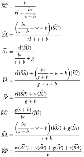
DFE
The second equilibrium, the disease-free equilibrium (DFE), has endemic sentiment but extinct disease ($\hat{I} = 0$ , $\hat{A} \gt 0$
 ). Variables with nonzero equilibrium values are

The equilibrium susceptible population for the DFE is

The two terms subtracted from 1 in eqn (9) reflect the two possible routes towards vaccination when sentiment is present (SU → SA → SP → RP and SU → SP → RP). The conflicting presence of the sentiment transmission rate c in the numerator and denominator of the term (s/c)(C 0 − 1) (recalling eqn 5 for C 0) reflects the fact that sentiment transmission and sentiment switching undermine each other but that sentiment switching only matters if sentiment is transmitted. In general, if pro-vaccine decisions are fast, sentiment transmission is slow or sentiment switching is fast, then most individuals will be vaccinated. If pro-vaccine decisions are slow, sentiment transmission is fast or sentiment switching is slow, then most individuals will be susceptible.
The DFE is stable if sentiment transmission outpaces pro-vaccine decision-making but disease transmission does not outpace vaccination (Table 3).
SFE
The third equilibrium, the sentiment-free equilibrium (SFE), has endemic disease but extinct sentiment ($\hat{I} \gt 0$ , $\hat{A} = 0$
 ). For this equilibrium, it is easiest to state the values of $\widehat{{SP}}$
 and $\hat{I}$
 and then write other nonzero values in terms of these two quantities. We have
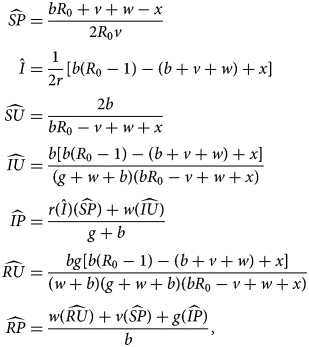
where

The SFE is stable if sentiment transmission does not outpace pro-vaccine decision-making but disease transmission outpaces vaccination (Table 3).
EE
The fourth equilibrium, the endemic equilibrium (EE), has both endemic disease and endemic anti-vaccine sentiment ($\hat{I} \gt 0$ , $\hat{A} \gt 0$
 ). The analytical form of this equilibrium is obtained by considering the real positive root of a quartic equation in $r\hat{I}$
 (Appendix A). From $r\hat{I}$
 , we divide by r to obtain $\hat{I}$
 , and from $\hat{I}$
 , we obtain $\widehat{{SP}}$
 :
:

From $\hat{I}$ and $\widehat{{SP}}$
 , we obtain all other quantities:
The EE is stable if sentiment transmission outpaces pro-vaccine decision-making and disease transmission outpaces vaccination (Table 3). This equilibrium potentially allows diseases with low transmission rates to be maintained in the population owing to the existence of anti-vaccine sentiment.
R 0and disease endemism
In the standard SIR model without vaccination (eqn 1, v = 0), the basic reproduction number R 0 (eqn 4) is the expected number of secondary cases of a disease produced by a typical infected individual in a population of susceptible individuals. This quantity determines the ultimate fate of the disease: if R 0 < 1, then the disease goes extinct, and if R 0 > 1, then the disease is endemic at equilibrium. With vaccination included in an SIR model with no anti-vaccine sentiment (eqn 1, v > 0), the criterion for disease endemism is

With vaccination present, R 0 can exceed 1, the threshold for disease maintenance in an unvaccinated population, but can fail to exceed 1 + v/b, so that the disease still goes extinct. By enlarging this threshold for R 0, vaccination makes it more difficult for the disease to persist.
Our model has two conditions for disease endemism, depending on whether sentiment is extinct or endemic. If sentiment is extinct at equilibrium, then the condition for disease endemism is

Here, we have rewritten the result from Table 3 to demonstrate that the critical value of R 0, the right-hand side of eqn (14), is always less than or equal to the critical value of R 0 for a system with vaccination but no sentiment dynamics: the right-hand side of eqn (13). No sentiment is present at equilibrium in this case, so the difference between eqns (14) and (13) is due to the presence of undecided, unvaccinated individuals. Their presence hinders the effects of vaccination, as it decreases the value of R 0 that the disease must achieve to be endemic. However, from eqn (14), the critical value of R 0 in this case is still always greater than or equal to 1. Thus, the presence of undecided, unvaccinated individuals resulting from sentiment dynamics maintains an R 0 critical value that lies between that of the model without vaccination and that of the model with vaccination but no sentiment.
If sentiment is endemic at equilibrium, then the condition for disease endemism is

The critical value of R 0, the right-hand side of eqn (15), is less than or equal to the critical value of R 0 in a system with vaccination but no sentiment – the right-hand side of eqn (13) – if s/(s + b) + (w − s)/c ≤ 1. This condition is equivalent to bc ≥ (s + b)(w − s), an inequality that is satisfied for the case with sentiment endemic at equilibrium: rearranging C 0 > 1 + w/b yields bc > (s + b)(w + b) > (s + b)w > (s + b)(w − s). Thus, as in the case with extinct sentiment (eqn 14), endemic anti-vaccine sentiment hinders the effects of vaccination by decreasing the critical value of R 0 that the disease must achieve to be endemic. Because all parameters in our model are nonnegative, and because s/(s + b) + (w − s)/c = (s/c)(C 0 − 1) + w/c and C 0 > 1, the denominator of the right-hand side of eqn (15) is always less than or equal to 1, so the critical value of R 0 in this case is always greater than or equal to 1. Thus, the effects of endemic sentiment also generate an R 0 critical value between that of the model without vaccination and that of the model with vaccination but no sentiment: the condition for disease spread in a scenario with vaccination and sentiment is stricter than in a model with no vaccination, but not as strict as with vaccination and no sentiment.
The right-hand side of eqn (15) is greater than or equal to that of eqn (14) if and only if bC 0 ≥ w + b. This condition is already satisfied with endemic sentiment (Table 3), so it is possible for a disease to be endemic if sentiment is endemic when it would not be endemic if sentiment were extinct.
Effects of parameters on stability of equilibria
We now study the effects of individual parameters on the stability of the equilibria. The compound parameters R 0 and C 0 in Table 3 suffice to determine whether or not an equilibrium is stable. To understand the effects of specific parameters, we visualize a subset of the parameter space. In particular, we focus on varying the sentiment parameters c, s and w, keeping the birth rate b and the disease parameters r, g and v fixed at values that represent well-studied diseases. As in standard SIR models in which r, g, and v are rate parameters that range from 0 to infinity (Hethcote, Reference Hethcote2000), the sentiment transmission rate c, the sentiment switching rate s, and the pro-vaccine decision rate w can range from 0 to infinity. We can therefore plot regions of the first quadrant of a plane considering two of these three variables to depict stability regions for the four equilibria. Figure 2 focuses on the c–w plane. The boundary curves in Figure 2 are derived in Appendix F.
Stability regimes for varying sentiment transmission rate c and pro-vaccine decision rate w. (a) R 0 ∈ [0, 1]. (b) $R_0\in \left({1\comma \;1{\rm /}\left[{1-{{sv} \over {\lpar {s + b} \rpar \lpar {v + b} \rpar }}} \right]} \right)$ . (c) $R_0\in \left[{1{\rm /}\left[{1-{{sv} \over {\lpar {s + b} \rpar \lpar {v + b} \rpar }}} \right]\comma \;1 + {v \over b}} \right)$
 . (d) $R_0\in \left[{1 + {v \over b}\comma \;\infty } \right)$
 . Parameter values for (a–d) are (b, g, v, s) = (0.002, 0.14, 0.14, 0.01). These parameters lead to transitional R 0 values of $1{\rm /}\left[{1-{{sv} \over {\lpar {s + b} \rpar \lpar {v + b} \rpar }}} \right] = 5.61$
 and 1 + v/b = 72.42. For (a), r = 0.1 so that R 0 = 0.69. For (b), r = 0.7 so that R 0 = 4.83. For (c), r = 1.5 so that R 0 = 10.36. For (d), r = 11 so that R 0 = 75.94. These parameter values were chosen so that the stability regions of all possible equilibria would be visible in each panel.

Note that in our model formulation, one might expect parameters w, the pro-vaccine decision rate, and c, the sentiment transmission rate, to be inherently inversely related, as a cultural environment with a high pro-vaccine decision rate could be incompatible with high transmissibility of anti-vaccine sentiment. Concurrently high values of w and c could arise with an underlying polarization in the population on the topic of vaccination, perhaps owing to political fracturing (e.g. Jegede, Reference Jegede2007; Dubé et al., Reference Dubé, Vivion and MacDonald2015) or the presence of a non-vaccinating religious community (e.g. Woudenberg et al., Reference Woudenberg, van Binnendijk, Sanders, Wallinga, de Melker, Ruijs and Hahné2017). Concurrently low values could arise in a situation of general indifference towards vaccines (e.g. Velan, Kaplan, Ziv, Boyko, & Lerner-Geva, Reference Velan, Kaplan, Ziv, Boyko and Lerner-Geva2011; MacDougall & Monnais, Reference MacDougall and Monnais2018). Thus, the two parameters are not necessarily inversely related and it is useful to consider the full c–w plane.
In Appendix F, it is shown that all parameter sets give rise to one of four regimes for the stability region in the c–w plane, with the regime determined by the value of R 0. The four cases correspond to four ranges for the value of R 0. The three R 0 values at which the regime transitions from one type to another are discussed in Appendix F.
First, if R 0 < 1, then the disease always goes extinct, and only the DSFE and DFE are possible (Figure 2a). This result is the same as in a standard SIR model, except that increasing the sentiment transmission rate c or decreasing the pro-vaccine decision rate w results in endemic sentiment.
Next, if

then the disease can spread in a completely susceptible population, and it is possible for the SFE and the EE to be stable in addition to the other two equilibria (Figure 2b). This case is most relevant for large values of the sentiment switching rate s, as the range of R 0 values that produce it is narrow for small s. As the sentiment transmission rate c increases, for large s, increased sentiment transmission increases vaccination in the population: many people transition from undecided to anti-vaccine and then, because of the high sentiment switching rate s, quickly become pro-vaccine. This situation, in which increased sentiment transmission can move the disease to extinction, represents a disease whose transmissibility cannot overcome the vaccination induced by sentiment switching after transmission of anti-vaccine sentiment.
Different behaviour occurs (Figure 2c) if

In this range, the disease is transmissible enough to overcome the increased vaccination induced by sentiment switching. Increasing the sentiment transmission rate c now makes the disease endemic.
Finally, if 1 + v/b ≤ R 0, then the disease is transmissible enough to overcome vaccination without assistance from anti-vaccine sentiment. In this situation, the DSFE and DFE are no longer stable anywhere, and decreasing vaccination by decreasing the pro-vaccine decision rate w or increasing the sentiment transmission rate c first leads to stability for the SFE and then for the EE.
Disease examples
To get a sense for which equilibria are stable in practical settings, we reproduce Figure 2 using disease parameter values that are commonly used to model polio (Figure 3a) and measles (Figure 3b). The parameter values appear in Table 4.
Stability regimes with parameter values chosen to represent two diseases. (a) Polio. (b) Measles. Parameter values are taken from Table 4. These values correspond to Figure 2c, where $R_0\in \left[{1{\rm /}\left[{1-{{sv} \over {\lpar {s + b} \rpar \lpar {v + b} \rpar }}} \right]\comma \;1 + {v \over b}} \right)$ . The sentiment-free equilibrium (SFE) is stable and lies in a region of the bottom-left corner of each plot, a region which is too small to see here.

Parameters for polio and measles. The disease transmission rate r is calculated from the basic reproduction number R 0, disease recovery rate g and birth rate b using eqn (4). Polio R 0, measles R 0 and measles g are taken from Anderson and May (Reference Anderson and May1991). Polio g is from Tebbens et al. (Reference Tebbens, Pallansch, Kew, Cáceres, Sutter and Thompson2005). The value of b is from Hamilton et al. (Reference Hamilton, Martin, Osterman, Curtin and Matthews2015). The value s = 0 is chosen for simplicity, and we expect s to be low in real populations. The value of v was chosen so that it takes about 7 days on average for a newly pro-vaccine individual to become vaccinated. The parameters r, g, v, and s are reported in units of days−1; b uses units of per capita births per day. R 0 is dimensionless. The values in the table were used to produce Figure 3

Parameter values for polio reside in case 3 (Figure 2c). Most of the parameter space in Figure 3a consists of regions where either the DSFE or the EE is stable, indicating a tight coupling between disease and sentiment endemism. In a non-trivial region where the DFE is stable, sentiment is endemic, but does not reduce vaccination sufficiently to permit disease to persist. A small region of Figure 3a where the SFE is stable is not visible but exists near the origin.
Parameter values for measles also reside in case 3 (Figure 2c). For measles, with a higher R 0 than polio, the regions in which either the DSFE or the EE is stable now occupy almost the entire parameter space in Figure 3b, indicating extremely tight coupling between disease and sentiment endemism. The high R 0 for measles couples the persistence of the disease to the persistence of sentiment, as disease can only persist in the population owing to sentiment endemism that reduces vaccination sufficiently for the disease to spread. This effect reflects a general result we derive in Appendix F: the greater the value of R 0, the larger the range of parameter values over which the DSFE or the EE is stable and the smaller the range over which the DFE or the SFE is stable.
Transient oscillations
Thus far, we have been examining equilibria of the model. We now turn our attention to the transient dynamics, solving eqn (2) numerically by specifying initial conditions and using a numerical differential-equation solver (see Appendix G). We begin with a population consisting primarily of susceptible individuals, so that an epidemic occurs early in the dynamics.
For parameter values that ultimately reach the endemic equilibrium, the transient dynamics are often oscillatory. We have observed two qualitatively different oscillation patterns in the transient dynamics of eqn (2). Figure 4 displays the patterns in three examples with initial compartment frequencies SU = 0.998 and IU = SA = 0.001.
Transient dynamics of the disease frequency for three different parameter sets. (a) Damped oscillation towards the endemic equilibrium (EE). The parameter values are (b, r, g, v, c, s, w) = (0.02, 0.8, 0.25, 0.2, 0.8, 0, 0.1). (b) Repeated epidemic spikes separated by long pauses. Parameter values are the same as in (a) except b = 0.0002. (c) Two epidemic regimes separated by a long pause during which the disease appears to go extinct. Parameter values are the same as in (a) except w = 0.25.

The first pattern (Figure 4a) is a damped oscillation around a stable EE. Comparably to a pattern sometimes seen in a standard SIR model (Wang et al., Reference Wang, Bauch, Bhattacharyya, d'Onofrio, Manfredi, Perc and Zhao2016), the amplitude of oscillation in the frequency of infected individuals becomes negligibly small after only a few cycles. In this example, the oscillatory pattern leads to two noticeable epidemics in a year, with the second less severe, before the disease reaches a relatively high endemic frequency (about 4%). The second pattern (Figure 4b) consists of large epidemics followed by periods in which the disease is nearly extinct. This example differs in that the birth rate b is smaller by a factor of 100, slowing the influx of undecided, susceptible individuals to such an extent that the disease frequency can only recover after long periods, when enough susceptible individuals have entered the population. This pattern is also observed in the standard SIR model when the endemic disease frequency is small and the system therefore has parameter values that give rise to the EE but are close to the region that produces the DFE (Wang et al., Reference Wang, Bauch, Bhattacharyya, d'Onofrio, Manfredi, Perc and Zhao2016). In this example, a series of epidemics occurs over a period of years, interrupting periods during which the disease is nearly extinct.
Figure 4c displays a situation that possesses both the damped oscillation around the EE from Figure 4a as well as the long pause between epidemics from Figure 4b. When extended over a longer period, the dynamics in Figure 4b in fact behave similarly to those in Figure 4c, with a damped oscillation to the EE, except that Figure 4b has multiple initial epidemic spikes rather than a single one, and the equilibrium disease frequency is small. Three epidemics occur over the course of a year, with the second more severe than the first and the third less dramatic than the second. During the period between the first two epidemics, the disease appears to be extinct. After the third epidemic, the disease settles into a relatively high endemic frequency (about 3%). In all cases in Figure 4, the disease goes extinct if the initial condition has no anti-vaccine sentiment.
Figure 5 further explores the dynamics of the oscillation seen in Figure 4c, showing the same dynamics but with more compartments. Figure 5a displays the disease-infected compartments IU, IA, IP and their total, I. The first epidemic at ~10 days consists of an increase in pro-vaccine IP individuals, suggesting that this epidemic is driven by pro-vaccine individuals getting infected with the disease before they have a chance to become vaccinated. This situation occurs because the initial population contains almost all disease-susceptible individuals.
Dynamics of compartments during long-pause oscillation behaviour. (a) Frequencies of disease-infected individuals of all sentiment classes and the total infected frequency. (b) Frequencies of disease-susceptible individuals of all sentiment classes and the total susceptible frequency. The dashed horizontal line is the 1/R 0 threshold frequency of disease-susceptible individuals necessary for the disease to spread. The parameter values follow Figure 4c.

In contrast, the second epidemic consists mostly of IA individuals, suggesting that this epidemic is driven by anti-vaccine individuals. The sentiment trajectories in Figure 5b support this claim, as an increase in the disease-susceptible, anti-vaccine compartment SA pushes the disease-susceptible frequency S above 1/R 0, the threshold necessary for the disease to spread.
Migration-triggered epidemics
In long pauses between oscillations such as those seen in Figure 4b and c, the disease drops to low frequencies. For instance, in the specific scenario shown in Figure 4c, the lowest disease frequency is 1.2 × 10⁻⁵. In practical settings, such low values might correspond to extinction of the disease. Thus, because disease prevalence can be effectively 0, we explored scenarios in which a single infected individual is reintroduced to the population.
Figure 6 considers introduction of a new disease case in a population of size 1000. We simulate this event by pausing the numerical solution of our model, instantaneously increasing disease frequency by 0.001, renormalizing the frequencies to sum to 1 and then completing the solution. From a baseline pattern similar to Figure 4c, the effect of this new case depends on when it is introduced. During the interval between the first two epidemics, when the disease is effectively extinct, a critical time exists at which the introduction quickly leads to an epidemic. The critical time is the time at which anti-vaccine sentiment has generated enough unvaccinated individuals that disease frequency would begin increasing in the absence of the new case (indicated by the time at which the frequency of susceptibles crosses the horizontal dashed line in Figures 6d–f).
Introducing a single new case of a disease into the population can affect the long-pause oscillation of the disease frequency differently, depending on when it is introduced. (a) Introduction early in the apparent extinction of the disease. (b) Introduction late in the apparent extinction of the disease. (c) Introduction after the disease has re-established and is oscillating towards an endemic equilibrium. (d–f) Disease-susceptible (S) and anti-vaccine (A) frequencies for the trajectories in (a–c). An arrow indicates the new case. In all panels, for the grey trajectory, provided as a reference, no new case is introduced. The vertical dashed line indicates the point at which disease frequency starts increasing after the initial epidemic, during its apparent extinction. The horizontal dashed line in (d–f) is the 1/R 0 threshold frequency of disease-susceptible individuals necessary for disease spread. Parameters used in this example are the same as in Figure 4c, except w is increased to 0.5 to provide a longer pause for illustration.

The grey trajectories in Figure 6a–c show the unperturbed disease frequency over time. In Figure 6a, a new case is introduced at day 250, prior to the critical time point, as the susceptible frequency lies below the threshold value in Figure 6d. The disease does not start epidemics, although the next epidemic does start earlier than without the new case. When the new case appears at day 1750 (Figure 6c), after the new epidemics have commenced and the susceptible frequency lies below the threshold value (Figure 6f), the oscillatory approach to endemic equilibrium is mildly perturbed but recovers quickly, with no lasting effect of the new case. However, when the new case appears at day 750 (Figure 6b), after the critical time point at which anti-vaccine sentiment has generated a sizeable population of unvaccinated individuals – indicated by the concurrent rise in the frequency of anti-vaccine sentiment and disease-susceptible individuals in Figure 6e – the new case immediately triggers epidemics. Thus, even if the disease effectively goes extinct, sentiment dynamics create a situation in which reintroducing a small number of infected individuals initiates new epidemics. In this specific example, such a migration immediately induces an epidemic only after a 15-month delay after the initial epidemic.
Assortative meeting
Homophily – or the tendency of like to interact with like – is a general property of human social behaviour (McPherson, Smith-Lovin, & Cook, Reference McPherson, Smith-Lovin and Cook2001). Vaccination behaviour exhibits homophily, so that anti-vaccine sentiment is not homogeneously distributed in populations (e.g. Salathé & Khandelwal, Reference Salathé and Khandelwal2011; Barclay et al., Reference Barclay, Smieszek, He, Cao, Rainey, Gao and Salathé2014; Onnela et al., Reference Onnela, Landon, Kahn, Ahmed, Verma, O'Malley and Christakis2016; Fu, Zimet, Latkin, & Joseph, Reference Fu, Zimet, Latkin and Joseph2019). We can extend our main model in eqn (2) to permit homophily through the phenomenon of assortative meeting (Eshel & Cavalli-Sforza, Reference Eshel and Cavalli-Sforza1982), modifying interaction probabilities by a parameter that increases the probability of interactions between individuals of the same sentiment class (A × A or P × P). The goal of this modification is to understand the influence of clustering in the population of anti-vaccine sentiment on the dynamics, as assortative meeting increases contacts among A individuals and among P individuals, and it decreases contacts between A and P individuals.
We consider an assortative meeting parameter α that affects the result of two draws with replacement from the population. We assume that undecided (U) individuals are unaffected by the rate of assortative meeting: if the first individual drawn is undecided (U), then the second draw is from the whole population. If the first individual drawn is anti-vaccine (A) or pro-vaccine (P), however, then the second draw is of type A or P, respectively, with probability α and it is from the whole population with probability 1 − α. Thus, α = 0 corresponds to the well-mixed case with no assortative meeting (eqn 2), and α = 1 corresponds to complete assortative meeting.
The new system of equations with this assortative meeting assumption is:
where

In eqn (17), I i for i = U, A, P represents a modified frequency of infected individuals available for interaction with an individual of sentiment type i (Appendix H). All three values reduce to I = IU + IA + IP if α = 0.
To examine the effect of assortative meeting on our model, we numerically solved eqn (16) using the measles parameters from Table 4 with c = 0.8, w = 0.14 and s = 0 (Appendix G). These values have the same order of magnitude as disease parameters r and v (Table 4) and lead to an endemic equilibrium (Figure 3). As an initial condition, we used SU = 0.06375, SA = 0.00525, IU = 0.001, RA = 0.06975 and RP = 0.86025, with other classes set to zero. We chose these initial frequencies to be near the 1 − 1/R 0 threshold for measles, RA + RP = 93% vaccine coverage, with overall anti-vaccine sentiment frequency SA + RA = 7.5%, the highest statewide rate of kindergarten non-medical vaccine exemptions in the US during 2017–2018 (Mellerson et al., Reference Mellerson, Maxwell, Knighton, Kriss, Seither and Black2018).
For a variety of values of α, Figure 7a shows this solution for the first 200 days, after which the initial epidemic has subsided. We see that a high value of α can trigger an epidemic that would otherwise not have occurred at α = 0. For high values of α, the epidemic is also shorter. Increased assortative meeting spreads disease within the anti-vaccine class, increasing the disease frequency; however, it also hinders both disease transmission to the undecided class and conversion of the undecided class to the anti-vaccine class, so that disease frequency drops quickly.
Disease frequency over time with various levels of assortative meeting. (a) Initial behaviour for a system that starts near the herd-immunity level for measles, with 7.5% of individuals having anti-vaccine sentiment. (b) Disease frequency after 50,000, 75,000 and 100,000 days for a system that starts at the endemic equilibrium. Both panels use measles parameters from Table 4 with c = 0.8 and w = 0.14. These values are chosen so that c is the same as that used in other analyses (Figures 4–6), w is on the same scale as v (Table 4) and the EE is stable (Table 3).

To study the effects of α on the equilibrium frequency of the disease, we numerically solved eqn (16) for 100,000 time steps interpreted as days, using the same parameters as in Figure 7a but starting at the endemic equilibrium for the original α = 0 model (eqn 2). The time period of 100,000 days was chosen to be long enough to rule out long-delayed epidemics.
Figure 7b plots the resulting values at 50,000, 75,000 and 100,000 time steps of the disease frequency I as a function of α. The disease frequency monotonically decreases with α, reflecting the pattern observed in Figure 7a that α speeds up the time at which disease becomes rare. In contrast to the dramatic effect the assortative meeting parameter α has on disease frequency in the short term (Figure 7a), its long-term effect is negligible (Figure 7b).
Discussion
We have studied a model of the joint dynamics of anti-vaccine sentiment and a vaccine-preventable disease, modelling the sentiment as a contagion itself: a cultural pathogen. We found that the disease and sentiment contagions have closely linked dynamics. The transient dynamics of anti-vaccine sentiment can cause repeated, easily triggered epidemics after long periods of disease absence. Presence of anti-vaccine sentiment and that of the disease are closely coupled: in general, at equilibrium, both are expected in the population or neither.
Consequences for anti-vaccine sentiment
We find that unless the disease would have been endemic in the absence of anti-vaccine sentiment, disease can always be eliminated at equilibrium through changes only in sentiment parameters. The DSFE appears in Figure 2a–c, and in most situations, a decrease in the sentiment transmission rate c or an increase in the pro-vaccine decision rate w enables the population to reach the DSFE and to eliminate disease. These results highlight the value of influencing sentiment behaviour as a management strategy for controlling disease.
Our analyses of specific disease parameters (Figure 3) revealed a difference between polio and measles owing to the greater R 0 for measles. In particular, we found that for diseases such as measles with high R 0, endemism of the disease is tightly coupled to endemism of anti-vaccine sentiment, so that the disease is only present if sentiment is present. For diseases with high R 0, it is thus particularly important to maintain low C 0 to avoid epidemics. The more transmissible the disease, the more important it is to decrease sentiment transmission.
The oscillations in Figures 4–6 demonstrate the power of sentiment dynamics to change transient disease dynamics. In Figure 5, sentiment dynamics force the system out of a sequence of oscillations or a steady approach to the DFE or EE, increasing disease frequency via sentiment spread.
Assortative meeting both intensifies epidemics and damps the spread of sentiment and disease. Under high assortativity, disease susceptibility is disproportionately found among anti-vaccine individuals. Individuals therefore only have a risk of becoming disease-infected if they have prolonged disease susceptibility owing to anti-vaccine sentiment; if undecided individuals do convert to the anti-vaccine class, then their risk of getting infected with the disease is dramatically increased.
The concentration of disease in the anti-vaccine class is not unlike scenarios with spatially localized disease reservoirs, such as nosocomial drug-resistant infections (e.g. Lipsitch, Bergstrom, & Levin, Reference Lipsitch, Bergstrom and Levin2000). Hospitalization is analogous to membership in the anti-vaccine class; similarly to the spread of disease in the anti-vaccine class by assortative meeting, assortative meeting of hospitalized individuals spreads drug-resistant strains of an infection within the hospital. In the non-hospitalized class, both susceptibility, via general overall health, and exposure, through assortative meeting with contacts who are generally non-hospitalized, are lower, so that disease remains largely localized.
Broadening the assumptions about transmission
Disease-behaviour analyses often examine highly structured populations in the form of networks. Our model instead focuses on a well-mixed population. This approach gives an analytically tractable model that can formalize qualitative results obtained from less tractable network models (e.g. Salathé & Bonhoeffer, Reference Salathé and Bonhoeffer2008). A well-mixed model also provides a baseline against which to compare more complicated structured population models. In our case, we were able to examine assortative meeting by sentiment type with a minor modification; other violations of the well-mixed-population assumption could also be analysed.
Our model fixes parameters for anti-vaccine sentiment transmission, examining the ensuing dynamics. Other studies have considered different aspects of vaccination behaviour. For example, game-theoretic studies that have modelled vaccine decision-making (e.g. Bauch & Earn, Reference Bauch and Earn2004; Fu, Rosenbloom, Wang, & Nowak, Reference Fu, Rosenbloom, Wang and Nowak2010) generally conclude that it is difficult to eliminate a disease from the population; when disease prevalence is low, reduced individual incentive to vaccinate increases disease prevalence. A second class of studies has modelled traits such as fear of a disease (e.g. Perra et al., Reference Perra, Balcan, Gonçalves and Vespignani2011) that induce transmission-reducing behaviours. These studies also find a relaxation of behavioural changes under low disease prevalence, leading to difficulties in long-term management of the disease. Although we did not include lethality from disease or a behavioural response to disease severity, our model accords with these previous results in finding that disease elimination is tied to disease-related behaviour – the elimination of sentiment. Even without feedback from disease prevalence to behaviour in the form of a direct impact on sentiment parameters, we still observe behaviourally driven disease rescue when the time-scale of sentiment transmission acts as an effective relaxation of disease-preventative behaviours (Figure 5). Our model therefore suggests that significant effects of anti-vaccine sentiment on disease dynamics can occur without complex mechanisms of sentiment uptake or transmission.
We did not consider a number of phenomena potentially relevant to sentiment transmission dynamics. Our transmission mechanism was constructed to be simple, with the cultural pathogen transmitted by contact in a well-mixed population. However, social contagions might require multiple interactions before transmission (e.g. Centola, Reference Centola2010), so that transmission mechanisms are not well approximated by an assumption of a single contact. Thus, for example, Pires and Crokidakis (Reference Pires and Crokidakis2017) adopted a majority-rule transmission mechanism in groups of three contacts. With multiple required interactions, Campbell and Salathé (Reference Campbell and Salathé2013) found that anti-vaccine sentiment can spread more slowly, but that the outbreaks can be more intense owing to the increased positive feedback tendencies of the sentiment spread. This and another study (Salathé & Bonhoeffer, Reference Salathé and Bonhoeffer2008) allowed opinion formation on a contact network, and found that increased opinion clustering dramatically increased the probability of an epidemic when the population was close to the minimal susceptible threshold needed to prevent outbreaks. Anti-vaccine sentiment can also be transmitted through centralized sources, such as governmental or media sources, with strong effects of such transmission on maintenance of deleterious cultural traits (Funk et al., Reference Funk, Salathé and Jansen2010; Yeaman, Schick, & Lehmann, Reference Yeaman, Schick and Lehmann2012); government or media transmission could be treated as a basis for spontaneous acquisition of anti-vaccine sentiment. Thus, the sentiment-only model of Hill, Rand, Nowak, and Christakis (Reference Hill, Rand, Nowak and Christakis2010) incorporates both transmissible sentiment and sentiment acquired by individual decision-making via spontaneous conversion. Permitting more sentiment compartments or using more complex contagion dynamics would extend the approach to cases with more detailed knowledge available about sentiment behaviours. A feedback of disease prevalence to sentiment dynamics (Goldstein, Philipson, Joo, & Daum, Reference Goldstein, Philipson, Joo and Daum1996; Bauch & Earn, Reference Bauch and Earn2004) would entail changing the constant sentiment transmission and pro-vaccine decision rates into decreasing and increasing functions of disease prevalence, respectively. This modification has the potential to create cyclic behaviour that is not observed in our current model.
Further modelling of sentiment transmission could also make use of mechanisms for social learning uncovered by the study of cultural transmission (e.g. Laland, Reference Laland2004; Mesoudi & Whiten, Reference Mesoudi and Whiten2008; Rendell et al., Reference Rendell, Fogarty, Hoppitt, Morgan, Webster and Laland2011; Hoppitt & Laland, Reference Hoppitt and Laland2013; Mesoudi, Reference Mesoudi2016). Beyond the simple ‘unbiased’ transmission (e.g. Cavalli-Sforza & Feldman, Reference Cavalli-Sforza and Feldman1981; Neiman, Reference Neiman1995) that we use, such mechanisms include conformity bias towards high-prevalence traits (e.g. Henrich & Boyd, Reference Henrich and Boyd1998; Reader, Bruce, & Rebers, Reference Reader, Bruce and Rebers2008; Muthukrishna, Morgan & Henrich, Reference Muthukrishna, Morgan and Henrich2016), payoff bias towards traits that appear to be better or that are exhibited by successful individuals (e.g. Boyd & Richerson, Reference Boyd and Richerson1985; Mesoudi, Reference Mesoudi2008; Tanaka et al., Reference Tanaka, Kendal and Laland2009; Henrich & Henrich, Reference Henrich and Henrich2010; Molleman, van den Berg, & Weissing, Reference Molleman, van den Berg and Weissing2014), and a mixture of social learning strategies in a heterogenous population (e.g. McElreath et al., Reference McElreath, Lubell, Richerson, Waring, Baum, Edsten and Paciotti2005; Efferson, Lalive, Richerson, McElreath, & Lubell, Reference Efferson, Lalive, Richerson, McElreath and Lubell2008).
Additional limitations and extensions
Other potential extensions include addition of age structure and the possibility of opposing social contagions. Age structure is important, as parents make vaccination decisions for children; parental decisions could be included by allowing new births to enter the population as anti-vaccine instead of undecided, at rates proportional to the prevalence of anti-vaccine sentiment among parents. Other ways of including parental decisions include a two-class population modelling approach with parents and children (Eames, Reference Eames2009) or a general age-structured co-infection approach (Castillo-Chavez, Hethcote, Andreasen, Levin, & Liu, Reference Castillo-Chavez, Hethcote, Andreasen, Levin and Liu1989).
Our model does not allow pro-vaccine individuals to transition to the undecided or anti-vaccine classes. This choice allowed us to interpret pro-vaccine sentiment as conferring immunity to anti-vaccine sentiment, enabling a perspective of a cultural inoculation against anti-vaccine sentiment (McGuire & Papageorgis, Reference McGuire and Papageorgis1961; Banas & Rains, Reference Banas and Rains2010). A model that permits the undecided class to be replenished by a conversion rate from the pro-vaccine class would be analogous to a SIRS model rather than an SIR model, as the class susceptible to the cultural pathogen can be re-entered (Hethcote, Reference Hethcote2000); this change could generate further oscillatory behaviour.
We also do not provide different rates for sentiment switching based on the disease state of an individual. For instance, anti-vaccine individuals who have been infected by the disease have the same rate of becoming pro-vaccine as those who have not been infected. In practice, sentiment switching could depend on disease state, with, for example, a higher sentiment-switching rate in the disease-infected class. However, adoption of vaccine-refusal behaviours is complex, potentially arising from reasons that are not related to the disease itself or leading to a preference for acquiring the disease rather than getting vaccinated (Dubé et al., Reference Dubé, Vivion and MacDonald2015; Reich, Reference Reich2016), so that sentiment-switching might have a complex relationship with disease state. A more general model that examines the relationship of vaccine refusal behaviours to disease state could potentially relax the assumption.
Our model also does not treat pro-vaccine sentiment as a contagion. This choice follows empirical evidence (Salathé et al., Reference Salathé, Vu, Khandelwal and Hunter2013), but does not preclude incorporation of a transmissible manner of expressing pro-vaccine sentiment. Understanding competing effects of transmissible pro-vaccine and anti-vaccine sentiment could facilitate analysis of the effects of a public policy that uses transmissible pro-vaccine sentiment as a management strategy.
For empirical application of our model, it would be possible to fit the sentiment model to observed trajectories of anti-vaccine sentiment prevalence and to then explore the effect that these dynamics would have on the corresponding disease, or perhaps on other diseases if anti-vaccine sentiment is correlated across diseases. Model-fitting to such data has been performed by Bauch and Bhattacharyya (Reference Bauch and Bhattacharyya2012), and sentiment trajectories could be obtained using social media in the manner of studies of Salathé and Khandelwal (Reference Salathé and Khandelwal2011) and Salathé et al. (Reference Salathé, Vu, Khandelwal and Hunter2013).
Conclusions
Early mathematical models of cultural evolution recognized the connection between cultural evolution and disease-transmission models, such as in analogies to susceptible, infected and resistant states for being unaware of a cultural trait, aware of the trait and having adopted the trait (Cavalli-Sforza & Feldman, Reference Cavalli-Sforza and Feldman1981). We find that using a direct analogy between a biological pathogen and a cultural pathogen generates an informative interaction between the two pathogens that in turn reveals distinctive dynamics in both the short term and the long term.
The formulation of the anti-vaccine sentiment transmission model as a cultural pathogen in an SIR framework identifies three quantities that affect sentiment dynamics and ultimately disease dynamics: the sentiment transmission rate c at which anti-vaccine sentiment is transmitted from the anti-vaccine class to the undecided class, the sentiment switching rate s at which the anti-vaccine class converts to pro-vaccine, and the pro-vaccine decision rate w at which the undecided class converts to pro-vaccine. Interventions to increase vaccination can potentially target any of these three types of transition – decreasing sentiment transmission to undecided individuals, increasing pro-vaccine decisions among undecided individuals, or increasing sentiment switching among anti-vaccine individuals. The influence of an intervention that produces a change of a given magnitude in one or more of these parameters can potentially be investigated using the model.
Finally, beyond our model, a cultural evolution approach can potentially facilitate examination of other questions raised by the existence of culturally pathogenic anti-vaccine sentiment. An analogy might exist with the virulence–transmissibility tradeoff in biological pathogens (Anderson & May, Reference Anderson and May1982; May & Anderson, Reference May and Anderson1983), by which high-virulence pathogens can evolve to be less transmissible than low-virulence pathogens. Such topics could be studied by permitting virulence and transmissibility of anti-vaccine sentiment to be influenced by virulence and transmissibility of the associated disease and studying coevolutionary dynamics over an evolutionary time scale.
Supplementary material
The supplementary material for this article can be found at https://doi.org/10.1017/ehs.2020.17.
Acknowledgements
We thank Marc Feldman for comments on the modelling of assortative meeting and Yoav Ram, Paul Smaldino, Mark Tanaka and an anonymous reviewer for comments on earlier versions of the manuscript.
Author contributions
R.S.M. and N.A.R. conceived and designed the study; R.S.M. performed the analysis; R.S.M. and N.A.R. revised the analysis and wrote the article.
Financial support
This research was supported by a graduate fellowship from the Center for Computational, Evolutionary and Human Genomics at Stanford University.
Conflict of interest
The authors declare that they have no conflicts of interest.
Data availability
All code used in the numerical analysis is available upon request.


 Open access