

1. Introduction
The Lambert Glacier–Amery Ice Shelf system (hereafter referred to as the “Lambert–Amery system”) is that part of the Antarctic ice sheet containing ice that drains through the front of the Amery Ice Shelf. Located at 68.5–81° S, 40–95° E, it is the largest glacier–ice-shelf system in East Antarctica. Until recently, few accurate elevation data existed for the system, and many of its important glaciological parameters were uncertain, including the mass balance and location of the grounding zone.
Satellite-radar altimeters are currently the most suitable instruments available for ice-sheet mapping at the desired accuracy and spatial and temporal resolution for climate-change studies. Two previous radar altimeter missions have provided topographic information over the Antarctic ice sheet north of 72.12° S: the US Navy’s Seasat mission (1978) and the Geosat mission (1985–90). Seasat and Geosat altimeter data have been used to generate digital elevation models (DEMs) of the Lambert–Amery system (e.g. Reference Herzfeld, Lingle and LeeHerzfeld and others, 1993; Reference Lingle, Lee, Zwally and SeissLingle and others, 1994) and of the Antarctic ice sheet (e.g. Reference Zwally, Bindschadler, Brenner, Martin and ThomasZwally and others, 1983; Reference Mantripp, Ridley and RapleyMantripp and others, 1992). On the Amery Ice Shelf, however, these satellite missions had a ground-track spacing of about 30 km, so topographic features, such as flow-related structures and meltstream channels, were poorly sampled.
The European Space Agency (ESA)’s European Remote-sensing Satellite (ERS-1) altimeter (1991–2000) is more suited to ice-sheet mapping than its predecessors for several reasons. Firstly, the ERS altimeter incorporated two modes of operation: an “ocean” mode, and an “ice” mode in which the operation was modified for use over ice-covered land surfaces. In ice mode, a more agile tracking algorithm and a wider range window meant that the altimeter had more chance of recording the echo from the ice surface which is rougher and steeper than the ocean surface. Secondly, the ERS-1 satellite provides measurements in the latitude range 82° N to 82° S. Finally, the mission completed two geodetic phases, with an orbit repeat period of 168 days, slightly shifted in longitude so that the ground tracks were interleaved. This meant that the separation of neighbouring ground tracks was only about 2–3 km on the Amery Ice Shelf, facilitating detailed topographic mapping.
This paper describes the generation of two DEMs for the Lambert–Amery system using ERS-1 geodetic-phase waveform data. The first is a 1 km DEM of the Amery Ice Shelf only, and the second is a 5 km DEM for the entire system. The DEMs are defined in the World Geodetic System 1984 (WGS84) coordinate system. DEMs of the Antarctic ice sheet have previously been generated from ERS-1 35 day fast delivery data (Reference Ridley, Laxon, Rapley and MantrippRidley and others, 1993; Reference BamberBamber, 1994) on a 20 km grid and from ERS-1 geodetic-phase waveform data (Reference Bamber and BindschadlerBamber and Bindschadler, 1997) on a 5 km grid. Our efforts at creating DEMs have followed similar procedures for waveform processing, but we have used a more accurate set of corrections, and more precise orbits. We have also been able to validate the DEMs against in situ GPS point positions and elevation profiles, collected during the 1994/95 Lambert Glacier basin (LGB) traverse (Reference Higham and CravenHigham and Craven, 1997) and the Amery Ice Shelf global positioning system (GPS) survey in 1995 (Reference Phillips, Allison, Coleman, Hyland, Morgan and YoungPhillips and others, 1998). To generate the DEM for the Amery Ice Shelf, we adopted a kriging procedure similar to that used by Reference Herzfeld, Lingle and LeeHerzfeld and others (1993), but we used anisotropic semivariograms to model more closely the spatial characteristics of the data along the ascending and descending track directions.
2. Altimeter Data Processing
The altimeter data used to construct the DEMs were collected during the two geodetic phases of ERS-1 (phases E and F, orbit numbers 14302–19247) between April 1994 and March 1995. The data obtained from ESA were in the Waveform Advanced Product (WAP) V2.0 format.
Satellite-radar altimeter data collected over ice need to be carefully processed in order to optimize the information content, because of the complex surfaces and scattering mechanisms involved. Our ERS-1 radar altimeter data-processing strategy comprised several steps, described below.
2.1. Waveform filtering
The ERS waveforms were filtered using four nested filters, which are described in the Appendix, to remove invalid cases. This allowed the whole waveform dataset to be analyzed using a uniform approach. Removal of specular returns at this stage also helped to avoid the inclusion of spurious elevation values caused by “snagging”, where the on-board tracker retained lock on the strong signal of the specular return to a considerable distance off-nadir rather than following the actual surface. Of the original waveforms over the region, 5.8% failed these four filter tests and were rejected, reducing the total number of altimeter measurement points to 10.4 × 10⁶
2.2. Incorporation of precise orbits
Uncertainty in the radial position of the ERS spacecraft introduces an error into the surface elevation derived from ERS altimeter measurements: the radial orbit error. We used precise orbits from the Delft University of Technology (Scharoo and Visser, 1998) to improve the accuracy of the ERS-1 spacecraft position. These orbits have a radial precision of approximately 90 mm.
Crossover analysis (section 2.7) was used to test for gross errors. This identified eight orbits with >30% of crossover differences greater than a threshold of 10 m, compared to a worst case of 2.5% for all other orbits. Another four orbits had rms values for the crossover differences (excluding the differences of > 10 m) that were more than four times the greatest rms value for all remaining orbits. All observations for these 12 orbits were deleted from the dataset. Large differences present in the remaining orbit set occur mainly over mountainous and steeply sloping surfaces.
2.3. Atmospheric corrections
Atmospheric corrections account for the retardation of the radar pulse by the Earth’s troposphere and ionosphere. ESA provides atmospheric corrections computed using physical models (Reference Cudlip and MilnesCudlip and Milnes, 1994). In theV2.0 WAP records, values of the dry tropospheric correction had been set to zero for elevations above approximately 2500 m, potentially leading to a height bias of around 1.8 m.
We used improved atmospheric corrections, based on local in situ observations, for the Lambert–Amery system (Reference Phillips, Allison, Coleman, Hyland, Morgan and YoungPhillips and others, 1998). Apart from where the dry tropospheric correction had been set to zero in the WAP records, the improved corrections made only a small difference to the altimeter range measurement. The sum of these corrections had a mean of 2.42 m, compared to a mean of 2.47 m from the WAP records.
2.4. Tide correction
The floating parts of the Antarctic ice sheet (ice shelves and glacier tongues) undergo vertical motion through the action of ocean tides. Static GPS measurements made on the Amery Ice Shelf in 1995 indicated that the height variation caused by tides was of order 1.5 m. Tidal observations were made using analogue and digital gauges in nearby Beaver Lake during a 23 day period in 1990/91 and a 30 day period in 1998. Beaver Lake is a small tidal lake west of the Amery Ice Shelf at about 70.8° S, 68.1° E. The Beaver Lake tide-gauge data were analyzed by the Australian National Tidal Facility to produce the Beaver Lake Tide Model (BLTM), which closely approximated (to within 10–50 mm) the height variation observed in the static GPS data on the ice shelf (Reference Phillips, Allison, Coleman, Hyland, Morgan and YoungPhillips and others, 1998). GPS measurements made on the ice shelf in 1998/99 indicated that the tidal displacement of the ice shelf varies spatially, and a phase lag should strictly be introduced depending on location on the shelf, but the BLTM is still a good first approximation.
In the ESA records, no tide values are given on the Amery Ice Shelf south of 70.5° S, which is >200 km north of the point where the ice shelf starts to float (73.2° S; Reference PhillipsPhillips, 1999). Hence we used the BLTM for all of our tidal corrections of altimeter data.
2.5. Retracking
“Retracking” corrects for the offset between the altimeter tracking point and the point on the waveform that corresponds to the mean surface (Reference Brenner, Bindschadler, Thomas and ZwallyBrenner and others, 1983). Retracking was carried out here using a threshold retracker with the threshold set at 25% of the mean of the returned power represented by a waveform (Reference Phillips, Allison, Coleman, Hyland, Morgan and YoungPhillips and others, 1998). The “mean” power was calculated using the same procedure as in the “offset centre-of-gravity” technique (Reference Wingham, Rapley and GriffithsWingham and others, 1986) but modified to use the square of the power (Reference Rapley, Guzkowska, Cudlip and MasonRapley and others, 1987).
2.6. Slope correction
The satellite-radar altimeter range measurement derived by the retracking procedure corresponds to the nearest point within its beam-limited footprint, which over sloping terrain does not correspond to nadir. This introduces a slope-induced error, which can be corrected using several techniques (Reference Brenner, Bindschadler, Thomas and ZwallyBrenner and others, 1983; Reference CooperCooper, 1989; Reference Remy, Mazzega, Houry, Brossier and MinsterRemy and others, 1989). Here we used Reference CooperCooper’s (1989) relocation technique. A database of slope values was compiled from the corrected and retracked altimeter data on a 10 km grid for the Antarctic continent. The slope of each gridcell was determined by fitting a plane to all data points falling within that gridcell. The slope correction was applied to each individual altimeter data point using a slope value interpolated from this database.
On the ice shelf itself, slope values range from around 0.02 at the front and in the centre to about 0.12° towards the southern end and around the edges. Therefore, typical relocation distances were of order 100 m, reaching 600 m in the steepest areas, with corresponding height adjustments of <0.5 m. It was difficult to assess the effectiveness of the slope correction over the ice shelf because it was within the rms of the altimeter data measurements.
2.7. Validation of radar altimeter data using crossover solutions
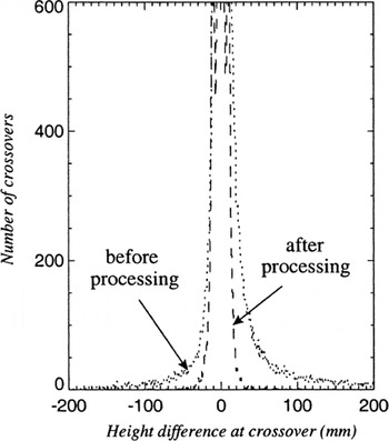
Crossover analyses were performed before and after data processing, to assess the improvement to the data integrity introduced by the processing scheme. Crossover analysis was performed on the altimeter data prior to the application of the slope correction because relocation of the data points complicates the determination of the crossover points. However, height differences at orbit intersections are independent of slope correction, because the magnitude of the slope-induced error is dependent only on the local surface slope, which is the same since the locations on the two tracks are coincident at the intersection.
Histograms of crossover differences over the Lambert–Amery system for the phase E and F data, before and after all of the processing steps described above (except slope correction) had been completed, are shown in Figure 1. Before processing, the rms of the height differences at the crossovers was 15.6 m; after processing, it reduced to 2.0 m. This shows that the processing considerably improves the internal consistency of the altimeter height measurements, and provides an estimate of the precision of the ERS data over the Lambert–Amery system.
Histogram of crossover differences (in m) between intersecting ERS-1 168 day ground-tracks over Lambert–Amery system before processing (dashed line) and after processing (dotted line).
2.8. Comparison of ERS-1 altimeter and GPS heights on the Amery Ice Shelf
The absolute accuracy of the ERS height measurement on the Amery Ice Shelf was assessed by comparing the altimeter data with “ground-truthing” data collected during the 1995 Amery Ice Shelf GPS survey (Reference Phillips, Allison, Coleman, Hyland, Morgan and YoungPhillips and others, 1998). A 120 km × 20 km grid, with individual gridcells 10 km on a side, was surveyed on the ice shelf using kinematic GPS. ERS- and GPS-derived surface heights were compared at the intersections of the ERS ground tracks with the GPS grid. The mean and rms of the height differences for all ERS-1 phase E and F tracks across the survey region were found to be 0.0 and 1.7 m, respectively. The spatial distribution of the height differences between the GPS and ERS altimeter data was highly correlated with surface topography.
3. Generation of DEMS
Two DEMs were generated from the validated ERS-1 satellite-radar altimeter data. The first was a high-resolution (1 km) DEM of the Amery Ice Shelf (AIS-DEM), and the second was a coarser-resolution (5 km) DEM of the entire Lambert–Amery system (LAS-DEM).
3.1. AIS-DEM
The method used to interpolate the ERS-1 altimeter data to create the AIS-DEM was “kriging” This is a geostatistical technique that produces a statistically unbiased, minimum error-variance data estimate at unobserved points of a surface from a set of observed points, provided that surface has spatially stationary statistics (Reference Deutsch and JournelDeutsch and Journel, 1992). The observed data are used to compute a “semivariogram”, which is a plot of semivariance as a function of distance between observations and thus describes the spatial variability of the observed data. In the application of the kriging process, the semivariogram is approximated by a model described by an analytical function fitted to the shape of the semivariogram. The model of the semivariogram is used in combination with the observed data to calculate estimates of the surface elevation at the grid nodes. Kriging is known as an “exact interpolator” because it maintains the data values at each of the observed points (Reference Deutsch and JournelDeutsch and Journel, 1992).
The ERS altimeter observations were converted to polar stereographic coordinates, with a standard parallel of latitude at 71° S and origin at the South Pole. For the Amery Ice Shelf, the x axis of the polar stereographic projection is closely aligned to the principal flow direction. Since the statistics are not stationary along the length of the Amery Ice Shelf, the AIS-DEM was created as four separate sections that overlapped in the x direction. The extent of each section was selected so that the spatial variability within the section was minimized, such that the statistics could be assumed to be spatially stationary. In this way the semivariogram would yield an unbiased estimate of the true height variability within that section. The x and y limits (in kilometres from the origin in the southeast corner (easting 4016 km, northing 5050 km)) for each of the four sections, AIS1–AIS4, are shown in Figure 2.
Contour plot of the AIS-DEM illustrating the locations of the four sections AIS1–AIS4, and the locations of the lines shown in Figure 4a and b. Contour intervals are 2 m for elevations of 10–110 m, 10 m for elevations of 110–210 m, and 20 m for elevations of >210 m.
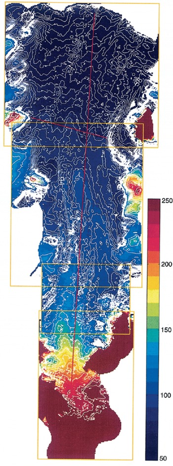
Since the surface statistics on the ice shelf are anisotropic, the ERS measurements in each section were used to compute directional semivariograms along the ascending (grid bearing 41.40) and descending (grid bearing 108.60) directions. The model fit to these semivariograms was determined using standard least-squares fitting routines. The semivariogram models were then used in the kriging routine, such that each region was interpolated separately on a 1 km grid. The four sections were combined to form the final AIS-DEM. A simple, distance-weighted averaging technique was used to join the sections so that the AIS-DEM was continuous across the overlap regions. The resulting AIS-DEM is presented as a contour plot in Figure 2, and a shaded surface perspective view in Figure 3.
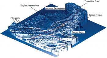
Shaded surface representation of the AIS-DEM. The features indicated are discussed in the main text. The locations of the lines shown in Figure 4a and b are indicated.
Striated pattern
The AIS-DEM (Fig. 3) contains a faint striated pattern on the surface. This pattern arises because of the non-random sampling of the surface by the altimeter tracks. Interpolated surface heights are simply a weighted average (as defined by the kriging process) of points within some neighbourhood. Therefore, interpolated heights between the altimeter tracks will be lower than the actual surface along ridges, and higher than the actual surface along valleys. This gives rise to a subtle saddle effect across the surface which is apparent because of its regularity.
Flowlines
Easily discernible in the AIS-DEM are longitudinal linear features that are parallel to the broad-scale ice-flow direction (Fig. 3). These are the main flow features of the ice shelf, arising from the merging of Lambert Glacier with other tributary glaciers such as Mellor and Fisher Glaciers at the southern end, Charybdis Glacier on the western flank, and numerous other smaller in-flows. Each of the major glaciers contributes a broad flow-band, which is several kilometres or more wide. The flow-bands generally exhibit slightly higher elevations in their main body than at their margins. Narrower features (a few hundred or more metres wide) can also be formed between neighbouring flow-bands where they merge. Such linear features, initiated by the ice flow, can correspond to flowlines. Quantitative information on flow features is provided in the AIS-DEM. Elevation maxima, which correspond to the flow-bands, are evident in profiles of surface elevations along straight lines oriented approximately along (south–north) and across (east–west) the ice shelf as presented in Figure 4. The locations of these lines are shown in Figures 2 and 3.

Grounding zone
The transition region of the Lambert–Amery system, the grounding zone, lies toward the southern limit of the AIS-DEM. This region has larger surface slopes than the remainder of the ice shelf where the ice moves from a grounded state to a free-floating state. The surface consists of bare ice, with variable topography, which results in noisier altimeter data, so the surface appears rougher in the AIS-DEM. Hydrostatic calculations indicate that the ice is floating as far south as 73.2° S (Reference PhillipsPhillips, 1999). There is a marked change in slope at 230–210 km in the longitudinal profile (Fig. 4a) around 100 m altitude (at 71.2° S) near Beaver Lake. This change in slope, originally observed with an optical levelling survey of the ice shelf in 1968, has been interpreted in previous work as the grounding line (e.g. Reference Budd, Corry and JackaBudd and others, 1982; Reference Partington, Cudlip, McIntyre and King-HelePartington and others, 1987; Reference Herzfeld, Lingle and LeeHerzfeld and others, 1993, Reference Herzfeld1997).
Surface depressions and flat regions
The AIS-DEM reveals distinct, long narrow surface depressions in the centre of the ice shelf, which are known to carry surface water during periods of snowmelt (Reference PhillipsPhillips, 1998). Other features revealed in the AIS-DEM are regions where the ice-shelf surface slopes are very small and the topography is flat (western section, near the ice front).
3.2. LAS-DEM
A second DEM was generated from the geodetic-phase ERS-1 data for the entire Lambert–Amery system, on a 5 km grid using a simple averaging technique. Each cell was assigned a mean height value, calculated from all the height values lying in that cell. Figure 5 is a nadir view plot of the LAS-DEM. Due to the nature of the terrain around the perimeter of the Amery Ice Shelf, there are no valid altimeter data in this area, nor over mountainous regions and rock outcrops, nor along coastal margins with large slopes.
Nadir view of LAS-DEM with shading. The light source is from directly above to highlight the surface slopes: flat surfaces appear white (such as on the tops of ridges and on the ice shelf) while steeply sloping surfaces appearas dark shades of blue. Areas coloured maroon correspond to where there were no data available due to the inability of the radaral timeter to retrieve a valid range measurement.
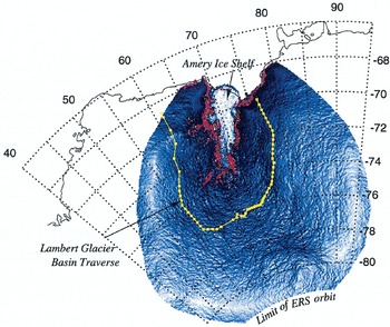
Figure 5 reveals a considerable amount of surface detail. The basin is clearly delineated by the ridges where the surface slope is very small, and major topographic features can also be seen. The area of the Lambert–Amery system is derived from the LAS-DEM as approximately 1550 400 km, with the boundary defined by the crests of the ridges and the flow-lines connecting the ridges to the front of the Amery Ice Shelf.
Validation of LAS-DEM with LGB traverse GPS data
Static GPS measurements made at 73 stations along the 1994/95 Australian National Antarctic Research Expedition LGB traverse (Reference Higham and CravenHigham and Craven, 1997; Reference Craven, Higham and BrocklesbyCraven and others, in press; Fig. 5) provide further validation for the LAS-DEM. Reference Manson, King and ColemanManson and others (1998) improved the height precision of the GPS data for 61 of the 73 stations and provided ellipsoidal heights in the WGS84 coordinate system. Although GPS heights are spot measurements, and therefore not directly comparable with altimeter-derived heights, the difference between the two sets of height values provides an indication of the accuracy of the LAS-DEM. At intermediate points between the GPS stations, approximately every 2–3 km along the traverse, elevations were also measured by differential barometric levelling. The barometric elevations have an accuracy of 1–2 m and give a good indication of the relative variability of the topography along the LGB traverse.
Figure 6a shows the height interpolated from the LAS-DEM at each of the intermediate measurement points along the LGB traverse, together with the measured elevations at each point (GPS and barometric). On the broad (10–50 km) scale, good agreement can be seen between the LAS-DEM heights and the GPS and barometric traverse heights. Figure 6b illustrates the differences in height along the LGB traverse route (LAS-DEM height minus measured height). The differences between the measured elevations at the stations and the corresponding LAS-DEM elevations have a mean of 12.2 m and an rms of 14.8 m.
(a) Comparison of interpolated elevations from the LAS-DEM (red) with GPS elevations at the 73 stations along the LGB traverse and the intermediate barometric heights (blue), (b) Height differences (LAS-DEM minus LGBT heights). (c) Expanded view of that part of the traverse between 150 and 300 km as indicated by the vertical lines in (a) and (b). (d) Expanded view of that part of the traverse between 650 and 800 km indicated by the vertical lines in (a) and (b).
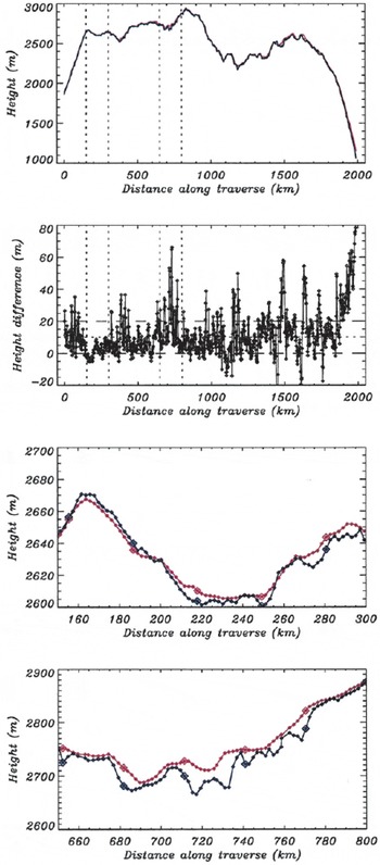
In Figure 6c and d, two 150 km long segments of the LGB traverse, indicated by the vertical lines in Figure 6b, have been enlarged. Figure 6c shows a segment containing small elevation differences, while Figure 6d shows large elevation differences. The barometric height profile is fairly smooth along the first segment, whereas the topography is quite variable on the 5–10 km scale (the order of the diameter of the altimeter footprint) in the second. Height differences are therefore correlated with fluctuations in the surface topography at the same order of the altimeter footprint size. The simple threshold retracking technique used here is unable to resolve all fluctuations in surface topography on the scale of the altimeter footprint, so an elevation bias is introduced, which has been discussed by other authors (Reference Gundestrup, Bindschadler and ZwallyGundestrup and others, 1986; Reference Wingham, Rapley and MorleyWingham and others, 1993). Careful processing of the altimeter data using a different retracking technique may overcome this effect.
4. Applications of the DEMS
The AIS-DEM has been combined with ice-thickness data in a buoyancy calculation to compute the location of the grounding zone of the ice shelf. Furthermore, the AIS-DEM has been used to delineate the regions of basal melting and freezing under the ice shelf. These applications are discussed in Reference PhillipsPhillips (1999) and will appear in later papers.
The coarse-scale LAS-DEM has applications in mass-balance studies in the Lambert–Amery system. This has been discussed in Reference PhillipsPhillips (1999) and is the subject of a companion paper in this journal (Reference Fricker, Warner and AllisonFricker and others, 2000). The LAS-DEM is also useful for ice-sheet dynamics studies, since it provides a reliable measurement of the magnitude of surface slope at the scale required for ice-sheet modelling. Using the LAS-DEM, Reference Warner and BuddWarner and Budd (2000) combined surface slopes with ice fluxes from mass-balance calculations and ice-sheet flow relations, to estimate the ice thickness and to infer, by further reference to the LAS-DEM, the bedrock topography of the grounded part of the Lambert–Amery system.
The DEMs presented here provide spatial context for field surveys which were conducted at discrete points or along lines. The new information allows results from historic surveys to be reassessed, correcting past misinterpretations such as the erroneous location of the Lambert–Amery grounding line. The DEMs and associated analyses also provide information critical to the planning and execution of studies of the Amery Ice Shelf. These include the selection of drilling sites to sample the basal conditions under the ice shelf, and the planning of current and future surveys to investigate its dynamics. The ice-thickness distribution derived from the AIS-DEM is being used, in combination with other data on the depth of the water column, to refine numerical models of the ocean tides under the shelf, which will contribute to understanding the dynamics and to improved resolution of the AIS-DEM.
5. Conclusions
Two DEMs have been created for the Lambert–Amery system from ERS-1 satellite-radar altimeter data. One DEM covers the floating part of the system (AIS-DEM, 1 km), and the other covers the whole system (LAS-DEM, 5 km). Both products have been computed in the WGS84 coordinate system and compared with in situ elevation data, so that their accuracy over the ice shelf and around the traverse route is known. The suitability of these DEMs for use in various applications, including hydrostatic studies (for grounding-zone definition, determination of the amount of melting and refreezing at the ice-shelf base), and balance-flux calculations has been demonstrated (Reference PhillipsPhillips, 1999; Reference Fricker, Warner and AllisonFricker and others, 2000).
Acknowledgements
The authors would like to acknowledge the LGB traverse team (M. Craven, R. Kiernan, A. Brocklesby, M. Higham) for the GPS data used to validate the LAS-DEM. We would also like to thank I. Allison, R. Manson and P. Morgan for their contributions to this work. Radar altimeter data from the ESA’s ERS satellites were provided as part of their Announcement of Opportunity Research Program through Project Id. ERS-A02-AUS103 (principal investigator N. Young). The altimeter data are Copyright ESA 1994 and 1995. All semivariogram computation and kriging was carried out using GAMV2 and KTB3D from Stanford University’s Geostatistical Software Library (Reference Deutsch and JournelDeutsch and Journel, 1992). This work was partly supported by funds from an Australian Research Council grant. Comments from S. Ekholm and an anonymous reviewer greatly improved the quality of the manuscript.
Appendix
This appendix contains descriptions of the filters used to remove erroneous waveforms from the ERS altimeter dataset collected over the Lambert–Amery system.
Leading-edge filter
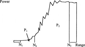
This filter removes waveforms where the leading edge is not recorded in the range window. Figure 7 demonstrates this filter.
Schematic diagram of the leading-edge filter. The range window is divided into two parts, and the powers in each part (P1 and P2) calculated. If P2 < T* P1, it is likely that the leading edge has not been recorded, and the waveform is rejected. The values used for N1, N2, N3 and T are 6, 13, 62 and 40 for ocean mode and 8, 19, 61 and 12 for ice mode, respectively.
Complex waveform filter
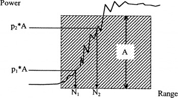
This filter removes waveforms whose shapes are too complex to produce useful height measurements, and is illustrated in Figure 8.
Schematic diagram of the complex waveform filter. The amplitude (A) of a box whose area is the same as the total integrated returned power is calculated. N1 is the bin whose power value first exceeds a percentage p1 of A, and N2 is the bin whose power value first exceeds a percentage p2 of A If N2 − N1 > T, the waveform is classed as complex, and rejected. The values used for N1, N2, p1, p2 and T are 6, 62, 15, 100 and 26 for ocean mode and 8, 61, 15, 100 and 12 for ice mode, respectively.
Specular waveform filter
This filter removes quasi-specular and specular waveforms, i.e. those in which the total power is contained within a small number of range bins, with a very high peak value. Over ice regions, these waveforms can arise from the highly reflective, flat surfaces of water bodies. The altimeter has a tendency to become “snagged” on such features for as long as they remain within its footprint, producing heights that can be underestimated by up to ∼30 m. Removal of these returns is essential for accurate elevation mapping over the ice shelf.
This filter uses the “pulse peakiness” (PP) (Reference Laxon and RapleyLaxon and Rapley, 1987), the maximum waveform amplitude (P max) the number of range bins (N) between 15% and 100% of the maximum power value for each waveform, and the backscatter (σ°). The rejection criteria for the filter are given in Table 1.
Criteria used for the simple quasi-specular return test
Negative backscatter filter
A further simple filter eliminated many instances of the problem of the altimeter “snagging” on surfaces of higher backscatter; for example, moving from the sea ice onto the continent, and moving from ice-shelf ice to grounded ice. This simple filter examines the radar backscatter (σ°) in dB from the altimeter record, and if σ° is negative the corresponding waveform is rejected.


