


1. Introduction
Loss reserving, the process of predicting the insurer’s outstanding liability, is a quintessential actuarial function in the insurance industry. Accurate estimation of loss reserves is crucial to several key operations within an insurance company, including claims management, ratemaking, and financial reporting (Frees, Reference Frees2015). Reserving methods can be broadly categorized into aggregate (macro) and individual (micro) approach, depending on the type of claims data utilized for model development. This work specifically concentrates on individual loss reserving methods tailored for multi-coverage insurance products.
Individual loss reserving methods were initially formulated within a marked Poisson process framework to accommodate granular claims data (see Arjas, Reference Arjas1989; Norberg, Reference Norberg1993, Reference Norberg1999). The first implementation of this model in empirical studies was due to Antonio and Plat (Reference Antonio and Plat2014). The point process approach is further extended to the marked Cox process to account for overdispersion (see Avanzi et al., Reference Avanzi, Wong and Yang2016; Badescu et al., Reference Badescu, Lin and Tang2016, Reference Badescu, Chen, Lin and Tang2019) and to a copula-based point process to accommodate informative terminal events (see Yang et al., Reference Yang, Shi and Huang2024). The core advantage of granular models lies in their ability to integrate detailed information into the forecasting process, including but not limited to case reserves (Taylor et al., Reference Taylor, McGuire and Sullivan2008), claim markers (i.e. claim-specific characteristics) (Godecharle and Antonio, Reference Godecharle and Antonio2015), and environmental changes (Okine, Reference Okine2023a). As claims data become more complex and voluminous, recent literature has witnessed the application of various machine learning methods in the context of individual loss reserving. Examples include Wüthrich (Reference Wüthrich2018), Lopez et al. (Reference Lopez, Milhaud and Thérond2019), Duval and Pigeon (Reference Duval and Pigeon2019), and Delong and Wüthrich (2020). We refer readers to the recent survey of Taylor (Reference Taylor2019) for detailed discussion on these developments.
Departing from the aforementioned literature, our work aims to develop an individual loss reserving method specifically designed for insurance policies providing multiple types of coverage. Multi-coverage contracts are prevalent in nonlife insurance, with examples such as automobile insurance indemnifying financial losses due to collision and third party liability (both property damage and bodily injury), homeowner insurance providing protection for building, contents, as well as liability, and workers compensation offering benefits for wage replacement, medical treatment, and vocational rehabilitation. A distinctive aspect of claims data from multi-coverage policies is the interrelation among claims from different coverage types. This unique feature demands careful consideration in the development of methodologies for individual loss reserving for multi-coverage policies. Despite the rapid expansion of the individual loss reserving literature, methods adept at accommodating dependence among multiple types of claims remain scarce. A recent example is Michaelides et al. (Reference Michaelides, Pigeon and Cossette2023) where the across-coverage dependence is introduced via activation patterns modeled with a multinomial logit regression while the loss amounts from different coverage types are treated as independent. Our research addresses this gap by proposing an individual loss reserving model that explicitly captures and quantifies the dependence among different types of claims originating from a multi-coverage insurance policy.
It is noteworthy that the underdevelopment of individual loss reserving methods for multi-coverage policies is in contrast to the extensive research on multivariate loss reserving methods in the aggregate context using loss triangle data. In the literature of aggregate loss reserving, various multivariate methods have been proposed to account for the dependence between different lines of business. Notable examples include nonparametric approaches such as those proposed by Merz and Wüthrich (Reference Merz and Wüthrich2008, Reference Merz and Wüthrich2009), and Zhang (Reference Zhang2010), and parametric approaches as evidenced by Shi and Frees (Reference Shi and Frees2011), Shi et al. (Reference Shi, Basu and Meyers2012), and De Jong (Reference De Jong2012). Given that dependence is a shared consideration for model development in both multi-coverage policies and multi-line insurance, one would naturally anticipate a parallel advancement in multivariate methods for individual reserving. Compared to the advanced state of multivariate aggregate loss reserving methods, the underdevelopment of individual loss reserving methods for multi-coverage insurance can be attributed to two primary reasons. First, from a methodology standpoint, the concept of dependence is well understood as an element-wise relationship in the context of multiple loss triangles. However, the notion of pairwise association becomes less clear when dealing with claim-level losses from multiple coverage types. Second, from a data perspective, access to granular loss data is more limited due to the constraints on data collection and data quality, and this issue is further compounded when considering claim data categorized by coverage type.
Furthermore, the development of multivariate granular reserving methods falls behind their ratemaking counterpart. It is widely recognized that pricing models in non-life insurance heavily rely on granular data driven by the competitive nature of the market. In particular, numerous multivariate pricing methods have been proposed for multi-coverage policies, such as automobile insurance (Frees and Valdez, Reference Frees and Valdez2008; Frees et al., Reference Frees, Shi and Valdez2009, and Shi et al., Reference Shi, Feng and Boucher2016) and commercial property insurance (Frees et al., Reference Frees, Lee and Yang2016). Additionally, these methods have been expanded for pricing multivariate insurance risks in a much broader sense, including multi-peril risks (Frees et al., Reference Frees, Meyers and Cummings2010; Shi and Yang, Reference Shi and Yang2018, and Yang and Shi, Reference Yang and Shi2019) and spatially correlated risks (Zhao et al., Reference Zhao, Shi and Feng2021 and Huang et al., Reference Huang, Zhang and Zhu2023). Beyond their application in reserving, individual loss reserving methods arguably play a more vital role in ratemaking (Crevecoeur et al., Reference Crevecoeur, Antonio, Desmedt and Masquelein2023 and Okine, Reference Okine2023b). Therefore, it is imperative to develop a multivariate individual loss reserving method to align with the demands of the ratemaking task.
In this paper, we present a copula-based granular reserving model designed for estimating loss reserves for multi-coverage insurance. Specifically, we employ a multivariate copula to jointly model the ultimate losses from different coverage types within a given claim, as well as the settlement time of the claim. Consequently, our proposed approach not only enables the quantification of dependence among losses of multiple coverage types but also captures the association between the size of the claim and its settlement time—a notable relationship identified in recent literature (see Okine et al., Reference Okine, Frees and Shi2022 and Yang et al., Reference Yang, Shi and Huang2024). The resulting model facilitates dynamic predictions for an insurer’s outstanding liability by leveraging information across coverage types and settlement delay. To tackle the estimation challenges due to imbalanced and censored observations in the data, we further introduce a stage-wise approach to estimate parameters in the proposed model. We investigate the efficacy of the stage-wise estimation using simulation studies and demonstrate dynamic prediction in a loss reserving application using a large portfolio of automobile insurance claims from a Canadian insurance company.
Lastly, it is worth commenting on the significant role of dependence in the individual reserving context. While the consideration of dependence among various types of losses is a shared aspect in both aggregate and individual loss reserving methods, its implications on reserve prediction are different. In the aggregate reserving context, neglecting dependence is detrimental to accurately quantifying reserving variability. In simpler terms, uncertainty is underestimated when losses are positively correlated and overestimated when losses are negatively correlated. In the proposed individual loss reserving model, dependence affects prediction uncertainty similarly. Moreover and of greater importance, accounting for dependence enables dynamic updating of predictions for the loss from one coverage type based on the loss development from other coverage types.
The rest of the article is organized as follows: Section 2 describes the granular claims data in automobile insurance that motivate our work. Section 3 introduces the copula-based individual loss reserving method for multi-coverage insurance. Section 4 delves into the two-stage estimation method through simulation studies. Section 5 applies the proposed method to the automobile insurance claims data and demonstrates dynamic prediction of outstanding claim payments. Section 6 concludes the paper.
2. Data
We consider a portfolio of private automobile insurance claims obtained from a Canadian insurance company, focusing on regions such as Ontario, Alberta, and the Atlantic provinces where mandatory coverages are not provided by public insurance companies. The portfolio consists of 563,426 insurance claims notified to the insurer between January 1st, 2015 and July 31st, 2021. The data contain detailed information for these claims collected by the insurer up to July 31st, 2021. It is important to note that not all claims have been settled by the end of our observation period.
Number and percentage of claims by coverage type.

Each insurance claim involves up to three types of coverage, automobile physical damage (APD), loss of use (LU), and bodily injury (BI). APD and LU cover the policyholder’s losses related to car damage and the need for a replacement car during repairs, respectively. BI compensates for third-party medical expenses when the insured is at fault. Notably, Canada’s public health insurance system limits medical expenses to what is not already covered, such as compensation for severe physical impairment or loss of income resulting from a car accident.
The dataset exhibits an imbalance wherein not all claims activate all three types of coverage. Table 1 provides a comprehensive overview of the combinations of coverage types within the insurance portfolio. It is evident from the table that the predominant portion of claims emanates from the APD coverage, with the majority of multi-coverage claims also being triggered by the APD coverage. This observation is expected, as LU and BI losses frequently follow APD losses in many cases.
The central outcome variables underpinning our analysis are the settlement time and loss amount. Within our context, settlement time refers to the period an insurer takes to process and settle an insurance claim subsequent to its reporting to the insurer, while loss amount indicates the ultimate losses delineated by coverage type. Table 2 offers descriptive statistics for these critical outcome variables. It is notable that both settlement time (measured in days) and loss amount (measured in CAD) exhibit right skewness and heavy-tailed distributions. Moreover, we observe that APD and LU claims are relatively high in frequency, although APD claims tend to have larger severity compared to LU claims. Additionally, BI claims occur less frequently, yet their loss severity surpasses that of the other two types of claims.
Descriptive statistics for settlement time and ultimate loss amount by coverage.

To investigate the relationship among these outcome variables, we present in Table 3 their pairwise associations using Kendall’s and Spearman’s rank correlation coefficients. Two types of associations are particularly pertinent to our study: the dependence among different types of coverage amounts and the dependence between settlement time and loss amount. The table reveals a positive correlation among losses of different coverage types. For instance, APD and LU exhibit a strong correlation, which can be reasonably explained by the fact that severe damage to the car necessitates a longer time for repairs. Moreover, the table illustrates a positive relationship between settlement time and loss amount. This positive correlation is also expected because larger claims typically take longer to settle due to the expertise and resources involved in the settlement process.
Pairwise rank correlation between settlement time and ultimate losses by coverage.

Furthermore, our dataset encompasses a rich array of both policy-level and claim-level information, serving as covariates in our analytical model. Table 4 summarizes the descriptive statistics of these predictors. All the covariates are presented as categorical variables with the percentage reported for each level. The majority of the covariates are policy-level attributes, which contain driver characteristics, such as age and gender, and metrics pertaining to the vehicle’s usage, such as its purpose and the distance driven. In addition, amidst these covariates, there is one claim-specific variable describing the degree of responsibility assigned for the accident.
Descriptive statistics for the covariates (percentage by level of each variable).

3. Methodology
3.1. Some notations
Consider an insurance policy offering k types of coverage. For a given insurance claim indexed by i, $T_i$
represents the settlement time, indicating the duration from the claim’s reporting to the insurer to its closure. Let
$T_i$
represents the settlement time, indicating the duration from the claim’s reporting to the insurer to its closure. Let $\eta_i^{(l)}$
, for
$\eta_i^{(l)}$
, for $l=1,\ldots,k$
, be a binary variable indicating whether the lth type of coverage is activated for the claim. At any given time
$l=1,\ldots,k$
, be a binary variable indicating whether the lth type of coverage is activated for the claim. At any given time $\tau$
during a claim’s progression, that is,
$\tau$
during a claim’s progression, that is, $\tau\in [0,T_i]$
, let
$\tau\in [0,T_i]$
, let $Y_i^{(l)}(\tau)$
represent the cumulative paid losses from coverage type l up to time
$Y_i^{(l)}(\tau)$
represent the cumulative paid losses from coverage type l up to time $\tau$
. Furthermore, we define the corresponding ultimate losses as
$\tau$
. Furthermore, we define the corresponding ultimate losses as $Y_i^{(l)}=Y_i^{(l)}(T_i)$
. In addition, denote baseline covariates as
$Y_i^{(l)}=Y_i^{(l)}(T_i)$
. In addition, denote baseline covariates as $\boldsymbol{x}_{i}=(X_{i1},\ldots,X_{ip})'$
.
$\boldsymbol{x}_{i}=(X_{i1},\ldots,X_{ip})'$
.
In our study, we operate under the assumption that the coverage information $\eta_i^{(l)}$
is available at the time of claim submission. That is, the insurer is able to identify coverage of all types when the claim is reported. It is important to note that this assumption should not be perceived as a limitation of our work. First, it is a reasonable assumption for personal automobile insurance and is corroborated by our dataset. Second, even if this assumption is not applicable in certain contexts, our proposed method remains valuable. In such cases, the method can be complemented by a separate model focused specifically on whether coverage of each type is triggered. In this work, we focus on reported claims. If one would like to model incurred but not reported (IBNR) losses, they could use our model in combination with a model predicting the number of not reported claims and their triggered coverage(s).
$\eta_i^{(l)}$
is available at the time of claim submission. That is, the insurer is able to identify coverage of all types when the claim is reported. It is important to note that this assumption should not be perceived as a limitation of our work. First, it is a reasonable assumption for personal automobile insurance and is corroborated by our dataset. Second, even if this assumption is not applicable in certain contexts, our proposed method remains valuable. In such cases, the method can be complemented by a separate model focused specifically on whether coverage of each type is triggered. In this work, we focus on reported claims. If one would like to model incurred but not reported (IBNR) losses, they could use our model in combination with a model predicting the number of not reported claims and their triggered coverage(s).
3.2. Joint model
Considering the interconnected nature of settlement time and loss amounts, we employ a multivariate regression framework to describe their relationship. Specifically, given covariates $\boldsymbol{X}_i$
, the (conditional) joint distribution function of
$\boldsymbol{X}_i$
, the (conditional) joint distribution function of $(Y_{i}^{(1)},\ldots,Y_{i}^{(k)},T_{i})$
, denoted by F, can be represented via a
$(Y_{i}^{(1)},\ldots,Y_{i}^{(k)},T_{i})$
, denoted by F, can be represented via a $(k+1)$
-variate copula as
$(k+1)$
-variate copula as
 \begin{align} & F(y_1,\ldots,y_k,t|\boldsymbol{X}_i) \nonumber \\[5pt] ={}& {\rm Pr}\big(Y_{i}^{(1)} \le y_1 ,\ldots, Y_{i}^{(k)}\le y_k ,T_{i} \lt t|\boldsymbol{X}_i\big) \nonumber \\[5pt] ={}& H(F_{1}(y_1|\boldsymbol{X}_i),\ldots,F_{k}(y_k|\boldsymbol{X}_i),F_{T}(t|\boldsymbol{X}_i)),\end{align}
where $F_l$
is the distribution function of
$F_l$
is the distribution function of $Y_{i}^{(l)}$
for
$Y_{i}^{(l)}$
for $l\in\{1,\ldots,k\}$
,
$l\in\{1,\ldots,k\}$
, $F_T$
is the distribution of
$F_T$
is the distribution of $T_i$
, and H is a
$T_i$
, and H is a $(k+1)$
-variate copula. Let
$(k+1)$
-variate copula. Let $\bar{H}$
denote the survival copula associated with H. We can express the joint survival function of
$\bar{H}$
denote the survival copula associated with H. We can express the joint survival function of $(Y_{i}^{(1)},\ldots,Y_{i}^{(k)},T_{i})$
, denoted by S, by
$(Y_{i}^{(1)},\ldots,Y_{i}^{(k)},T_{i})$
, denoted by S, by
 \begin{align} & S(y_1,\ldots,y_k,t|\boldsymbol{X}_i) \nonumber\\[5pt] ={}& {\rm Pr}\big(Y_{i}^{(1)} \gt y_1 ,\ldots, Y_{i}^{(k)}\gt y_k ,T_{i} \gt t|\boldsymbol{X}_i\big) \nonumber\\[5pt] ={}& \bar{H}(1-F_{1}(y_1|\boldsymbol{X}_i),\ldots,1-F_{k}(y_k|\boldsymbol{X}_i),1-F_{T}(t|\boldsymbol{X}_i)).\end{align}
Next, we delineate the marginal models for $Y_{i}^{(l)}$
and
$Y_{i}^{(l)}$
and $T_{i}$
. We employ parametric regression model for the specification of the ultimate payment
$T_{i}$
. We employ parametric regression model for the specification of the ultimate payment $Y_i^{(l)}$
, for
$Y_i^{(l)}$
, for $l\in\{1,\ldots,k\}$
, and an accelerated failure time model (AFT) for the settlement time
$l\in\{1,\ldots,k\}$
, and an accelerated failure time model (AFT) for the settlement time $T_{i}$
. Specifically, the marginal model for the loss amount is expressed as
$T_{i}$
. Specifically, the marginal model for the loss amount is expressed as
 \begin{align*} &Y_i^{(l)}|\boldsymbol{X}_i \sim F_l\big(y;\; \mu^{(l)}_i, \boldsymbol{\phi}_l\big) \\[5pt] & \mu^{(l)}_i= s_l\big(\boldsymbol{X}_i;\; \boldsymbol{\alpha}^{(l)}\big),\end{align*}
where $\mu^{(l)}_i$
denotes the location parameter and is further modeled through a smooth function
$\mu^{(l)}_i$
denotes the location parameter and is further modeled through a smooth function $s(\cdot;\;\boldsymbol{\alpha})$
with parameters
$s(\cdot;\;\boldsymbol{\alpha})$
with parameters $\boldsymbol{\alpha}$
, and
$\boldsymbol{\alpha}$
, and $\boldsymbol{\phi}_l$
denotes additional parameters that is assumed constant.
$\boldsymbol{\phi}_l$
denotes additional parameters that is assumed constant.
The marginal model for the settlement time is given by
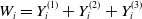
 \begin{align*} &\log(T_i) = \zeta(\boldsymbol{X}_i;\;\boldsymbol{\beta}) + \sigma W_i\\[5pt] & W_i|\boldsymbol{X}_i \stackrel{i.i.d.}\sim F_0,\end{align*}
where $F_0$
belongs to a log-location-scale family. Under the AFT model, we have
$F_0$
belongs to a log-location-scale family. Under the AFT model, we have
 \begin{align*} F_T(t|\boldsymbol{X}_i) = F_0\left(\frac{\log(t)-\zeta(\boldsymbol{X}_i;\;\boldsymbol{\beta})}{\sigma}\right)\!.\end{align*}
In above, $\zeta(\cdot;\;\boldsymbol{\beta})$
is a smooth function parameterized by
$\zeta(\cdot;\;\boldsymbol{\beta})$
is a smooth function parameterized by $\boldsymbol{\beta}$
. In both the GLM and AFT, we consider the special case of a linear model, that is,
$\boldsymbol{\beta}$
. In both the GLM and AFT, we consider the special case of a linear model, that is, $s_l(\boldsymbol{X}_i;\; \boldsymbol{\alpha}^{(l)})=\boldsymbol{X}'_i\boldsymbol{\alpha}^{(l)}$
and
$s_l(\boldsymbol{X}_i;\; \boldsymbol{\alpha}^{(l)})=\boldsymbol{X}'_i\boldsymbol{\alpha}^{(l)}$
and $\zeta(\boldsymbol{X}_i;\; \boldsymbol{\beta})=\boldsymbol{X}'_i\boldsymbol{\beta}$
. Note that an intercept should be included in the linear model.
$\zeta(\boldsymbol{X}_i;\; \boldsymbol{\beta})=\boldsymbol{X}'_i\boldsymbol{\beta}$
. Note that an intercept should be included in the linear model.
Lastly, we utilize a $(k+1)$
-variate Gaussian copula with an unstructured correlation matrix. We denote the Gaussian copula as
$(k+1)$
-variate Gaussian copula with an unstructured correlation matrix. We denote the Gaussian copula as
 \begin{align} H(u_1,\ldots,u_k,u_{k+1}) = \Phi_{k+1}(\Phi^{-1}(u_1),\ldots,\Phi^{-1}(u_k),\Phi^{-1}(u_{k+1});\;\boldsymbol{\Sigma}),\end{align}
where $\boldsymbol{\Sigma}$
is the
$\boldsymbol{\Sigma}$
is the $(k+1)\times(k+1)$
correlation matrix. The Gaussian copula is most commonly used in multivariate analysis. The selection of the copula is a balance of interpretability, model complexity, and computational efficiency. In particular, the following two properties of the Gaussian copula are desirable for our method. First, the copula is symmetric such that
$(k+1)\times(k+1)$
correlation matrix. The Gaussian copula is most commonly used in multivariate analysis. The selection of the copula is a balance of interpretability, model complexity, and computational efficiency. In particular, the following two properties of the Gaussian copula are desirable for our method. First, the copula is symmetric such that $\bar{H}=H$
. Second, consider the partial derivatives for
$\bar{H}=H$
. Second, consider the partial derivatives for $l=1,\ldots,k-1$
:
$l=1,\ldots,k-1$
:
 \begin{align*} \partial_{l:T}\bar{H}(u_1,\ldots,u_k,u_{k+1}) = \frac{\partial^{l+1}}{\partial u_1 \cdots \partial u_l\partial u_{k+1}} \bar{H}(u_1,\ldots,u_k,u_{k+1}).\end{align*}
Straightforward calculations show:
 \begin{align*} & \partial_{l:T}\bar{H}(u_1,\ldots,u_k,u_{k+1})\\[5pt] ={}& \Phi_{k-l}\big(\big(\boldsymbol{\Sigma}_{22}-\boldsymbol{\Sigma}_{21}\boldsymbol{\Sigma_{11}}^{-1}\boldsymbol{\Sigma}'_{21}\big)^{-1/2}\big({\boldsymbol{z}}_2-\boldsymbol{\Sigma}_{21}\boldsymbol{\Sigma}^{-1}_{11}{\boldsymbol{z}}_1\big)\big) \cfrac{\phi_{l+1}({\boldsymbol{z}}_1)}{\phi\big(\Phi^{-1}(u_1)\big)\cdots\phi\big(\Phi^{-1}(u_l)\big)\phi\big(\Phi^{-1}(u_{k+1})\big),} \end{align*}
where for $l=1,\ldots,k-1$
:
$l=1,\ldots,k-1$
:
 \begin{align*} {\boldsymbol{z}}_1&=\big(\Phi^{-1}(u_1),\ldots,\Phi^{-1}(u_l),\Phi^{-1}(u_{k+1})\big) \\[5pt] {\boldsymbol{z}}_2&=\big(\Phi^{-1}(u_{l+1}),\ldots,\Phi^{-1}(u_k)\big),\end{align*}
and
 \begin{align*}\boldsymbol{\Sigma}_{11} &= \left(\begin{array}{c@{\quad}c@{\quad}c@{\quad}c@{\quad}c} 1 & \rho_{12} & \cdots & \rho_{1l} & \rho_{1,k+1} \\[5pt] \rho_{12} & 1 &\cdots & \rho_{2l} & \rho_{2,k+1} \\[5pt] \vdots & \vdots & \ddots & \vdots & \vdots \\[5pt] \rho_{1l} & \rho_{2l} & \cdots & 1 & \rho_{l,k+1} \\[5pt] \rho_{1,k+1} & \rho_{2,k+1} & \cdots & 1 & 1 \\[5pt] \end{array}\right),\\[5pt] \boldsymbol{\Sigma}_{21}& = \left(\begin{array}{c@{\quad}c@{\quad}c@{\quad}c} \rho_{1,l+1} & \cdots & \rho_{l,l+1} & \rho_{l+1,k+1}\\[5pt] \vdots & \ddots & \vdots & \vdots \\[5pt] \rho_{1,k} & \cdots & \rho_{l,k} & \rho_{k,k+1} \\\end{array}\right), \;\boldsymbol{\Sigma}_{22} = \left(\begin{array}{c@{\quad}c@{\quad}c@{\quad}c} 1 & \rho_{l+1,l+2} & \cdots & \rho_{l+1,k} \\[5pt] \rho_{l+1,l+2} & 1 & \cdots & \rho_{l+2,k} \\[5pt] \vdots & \vdots & \ddots & \vdots \\[5pt] \rho_{l+1,k} & \rho_{l+2,k} & \cdots & 1 \\\end{array}\right)\!.\end{align*}
One can observe that the modeling approach does not incorporate the timing or amount of individual partial payments. Instead, only the total cumulative partial payment at the time of valuation is considered. All models involve trade-offs, with assumptions that bring both strengths and limitations. Our modeling choice can be viewed as a limitation, but not necessarily in all contexts. First, the data on the individual payment amounts and timing can be noisy, often reflecting operational variability (e.g., adjuster behavior or insurer accounting practices) rather than characteristics that are directly related to the ultimate loss. In such cases, modeling these payment paths explicitly could introduce more noise than signal. Our approach, by focusing on cumulative partial payments, may offer greater robustness to such misspecification. Second, even models that explicitly incorporate individual payment-level data are not guaranteed to yield distinct predictions, as sufficient statistics—such as the cumulative partial payment—can effectively summarize the relevant information. Consequently, the absence of finer-grained data does not inherently entail a loss in predictive power. We do not claim that our proposed method is universally superior; rather, our goal is to offer a flexible and interpretable addition to the growing toolbox of individual loss reserving methods available to actuaries.
3.3. Estimation
In practice, it is common for reserving models to be trained prior to the valuation date, where the insurer’s book of claims typically comprises both open and closed claims. Let us consider a portfolio of n insurance claims. We denote $C_i$
as the valuation time (from the reporting to the valuation) associated with the ith claim
$C_i$
as the valuation time (from the reporting to the valuation) associated with the ith claim $(i=1,\ldots,n)$
. It is worth noting that for a common valuation time for the portfolio,
$(i=1,\ldots,n)$
. It is worth noting that for a common valuation time for the portfolio, $C_i$
could be claim specific due to different reporting times. We define
$C_i$
could be claim specific due to different reporting times. We define ${\delta_i} = \textbf{1}(T_i\le C_i)$
. Furthermore, we define
${\delta_i} = \textbf{1}(T_i\le C_i)$
. Furthermore, we define $\tilde{T}_i = \min\{T_i,C_i\}$
and
$\tilde{T}_i = \min\{T_i,C_i\}$
and $\tilde{Y}_{i}^{(l)}=Y_{i}^{(l)}(\tilde{T}_i)=\min\{Y_{i}^{(l)}(T_i),Y_{i}^{(l)}(C_i)\}$
. This last relation assumes that the outstanding liabilities, net of recoveries, are positive. Denote
$\tilde{Y}_{i}^{(l)}=Y_{i}^{(l)}(\tilde{T}_i)=\min\{Y_{i}^{(l)}(T_i),Y_{i}^{(l)}(C_i)\}$
. This last relation assumes that the outstanding liabilities, net of recoveries, are positive. Denote $\tilde{\boldsymbol{Y}}_i=(\tilde{Y}_{i}^{(1)},\ldots,\tilde{Y}^{(k)}_{i})'$
and
$\tilde{\boldsymbol{Y}}_i=(\tilde{Y}_{i}^{(1)},\ldots,\tilde{Y}^{(k)}_{i})'$
and $\boldsymbol{\eta}_{i} = (\eta_{i}^{(1)},\ldots,\eta_{i}^{(k)})$
. To facilitate presentation of the density and survival functions for different coverage combination in a general form, we define
$\boldsymbol{\eta}_{i} = (\eta_{i}^{(1)},\ldots,\eta_{i}^{(k)})$
. To facilitate presentation of the density and survival functions for different coverage combination in a general form, we define $\boldsymbol{v}=(v_1,\ldots,v_k)$
, where
$\boldsymbol{v}=(v_1,\ldots,v_k)$
, where $v_l \in\{0,1\}$
for
$v_l \in\{0,1\}$
for $l=1,\ldots,k$
(analogous to
$l=1,\ldots,k$
(analogous to $\boldsymbol{\eta}_{i}$
), and introduce:
$\boldsymbol{\eta}_{i}$
), and introduce:
 \begin{align} g(u_1,\ldots,u_k,u_{k+1}|\boldsymbol{v}) = \frac{\partial^{\sum_{l=1}^k v_l +1}}{\partial u_1^{v_1} \cdots, \partial u_k^{v_k} \partial u_{k+1}}H\big(u_1^{v_1},\ldots,u_k^{v_k},u_{k+1} \big) \end{align}
 \begin{align} \bar{G}(u_1,\ldots,u_k,u_{k+1}|\boldsymbol{v}) = \bar{H}\big(u_1^{v_1},\ldots,u_k^{v_k},u_{k+1}\big).\end{align}
Denote the vector of model parameters as $\boldsymbol{\theta}=(\boldsymbol{\theta}_1,\ldots,\boldsymbol{\theta}_k,\boldsymbol{\theta}_{T},\boldsymbol{\theta}_{\Sigma})$
, where
$\boldsymbol{\theta}=(\boldsymbol{\theta}_1,\ldots,\boldsymbol{\theta}_k,\boldsymbol{\theta}_{T},\boldsymbol{\theta}_{\Sigma})$
, where $\boldsymbol{\theta}_l$
,
$\boldsymbol{\theta}_l$
, $l=1,\ldots,k$
, represents the parameter vector in the marginal model of
$l=1,\ldots,k$
, represents the parameter vector in the marginal model of $Y_i^{(l)}$
,
$Y_i^{(l)}$
, $\boldsymbol{\theta}_{T}$
is the parameter vector in the marginal model of
$\boldsymbol{\theta}_{T}$
is the parameter vector in the marginal model of $T_i$
, and
$T_i$
, and $\boldsymbol{\theta}_{\Sigma}$
denotes the parameter vector in the copula. Let
$\boldsymbol{\theta}_{\Sigma}$
denotes the parameter vector in the copula. Let $\mathcal{D}_n=\{\boldsymbol{X}_i,\delta_i,\boldsymbol{\eta}_{i},\tilde{t}_i, \tilde{{\boldsymbol{y}}}_{i}\;:\; i=1,\ldots,n\}$
be the data available by the valuation, which contains information on valuation time, claim status, and settlement time for closed claims, along with baseline covariates. The overall loglikelihood function for the data can be expressed as
$\mathcal{D}_n=\{\boldsymbol{X}_i,\delta_i,\boldsymbol{\eta}_{i},\tilde{t}_i, \tilde{{\boldsymbol{y}}}_{i}\;:\; i=1,\ldots,n\}$
be the data available by the valuation, which contains information on valuation time, claim status, and settlement time for closed claims, along with baseline covariates. The overall loglikelihood function for the data can be expressed as
 \begin{align} \mathcal{L}(\boldsymbol{\theta}) = \sum_{i=1}^n \left\{\delta_i \log f\big(\tilde{y}_{i}^{(1)},\ldots,\tilde{y}_{i}^{(k)},\tilde{t}_i|\boldsymbol{X}_i,\boldsymbol{\eta}_{i}\big) + (1-\delta_i) S\big(\tilde{y}_{i}^{(1)},\ldots,\tilde{y}_{i}^{(k)},\tilde{t}_i|\boldsymbol{X}_i,\boldsymbol{\eta}_{i}\big)\right\}\!,\end{align}
where
 \begin{align*} f\big(\tilde{y}_{i}^{(1)},\ldots,\tilde{y}_{i}^{(k)},\tilde{t}_i|\boldsymbol{X}_i,\boldsymbol{\eta}_{i}\big) &= f_{T}(\tilde{t}_i|\boldsymbol{X}_i) \prod_{l=1}^k \left\{f_{l}\big(\tilde{y}_{i}^{(l)}|\boldsymbol{X}_i\big)\right\}^{\eta_i^{(l)}} \\[5pt] & \;\;\;\;\times g\big(F_{1}\big(\tilde{y}_{i}^{(1)}|\boldsymbol{X}_i\big),\ldots,F_{k}\big(\tilde{y}_{i}^{(k)}|\boldsymbol{X}_i\big),F_{T}(\tilde{t}_i|\boldsymbol{X}_i)|\boldsymbol{\eta}_{i}), \\[5pt] S\big(\tilde{y}_{i}^{(1)},\ldots,\tilde{y}_{i}^{(k)},\tilde{t}_i|\boldsymbol{X}_i,\boldsymbol{\eta}_{i}\big) &= \bar{G}\big(1-F_{1}\big(\tilde{y}_{i}^{(1)}|\boldsymbol{X}_i\big),\ldots,1-F_{k}\big(\tilde{y}_{i}^{(k)}|\boldsymbol{X}_i\big),1-F_{T}(\tilde{t}_i|\boldsymbol{X}_i)|\boldsymbol{\eta}_{i}\big).\end{align*}
The model parameters can be estimated using the full information likelihood approach by directly maximizing the overall log-likelihood function defined by (3.6). However, the maximum likelihood estimation could be computationally inefficient and impractical. To address this issue, we propose a stage-wise estimation method to implement the full information likelihood in a computationally efficient manner. Let us denote $\boldsymbol{\theta}_{\Sigma_{YT}} = \{\theta_{lT}\;:\; l = 1,\ldots,k\}$
where
$\boldsymbol{\theta}_{\Sigma_{YT}} = \{\theta_{lT}\;:\; l = 1,\ldots,k\}$
where $\theta_{lT}$
describes the dependence between
$\theta_{lT}$
describes the dependence between $Y_i^{(l)}$
and
$Y_i^{(l)}$
and $T_i$
, and
$T_i$
, and $\boldsymbol{\theta}_{\Sigma_{YY}} = \{\theta_{ll'}\;:\; l, l'= 1,\ldots,k \;{\rm and}\; l \lt l' \}$
where
$\boldsymbol{\theta}_{\Sigma_{YY}} = \{\theta_{ll'}\;:\; l, l'= 1,\ldots,k \;{\rm and}\; l \lt l' \}$
where $\theta_{ll'}$
describes the dependence between
$\theta_{ll'}$
describes the dependence between $Y_i^{(l)}$
and
$Y_i^{(l)}$
and $Y_i^{(l')}$
. Further denote
$Y_i^{(l')}$
. Further denote $\boldsymbol{\theta}_{\Sigma} =(\boldsymbol{\theta}_{\Sigma_{YT}}, \boldsymbol{\theta}_{\Sigma_{YY}})$
. Let
$\boldsymbol{\theta}_{\Sigma} =(\boldsymbol{\theta}_{\Sigma_{YT}}, \boldsymbol{\theta}_{\Sigma_{YY}})$
. Let $H_{l:T}$
be the bivariate copula associated with
$H_{l:T}$
be the bivariate copula associated with $(Y_i^{(l)}, T_i)$
, that is
$(Y_i^{(l)}, T_i)$
, that is
 \begin{align*} H_{l:T}(u_l,u_{k+1}) = H(1,\ldots,1,u_l,1,\ldots,1,u_{k+1}), \;{\rm for}\; l=1,\ldots,k.\end{align*}
And let $h_{l:T}$
and
$h_{l:T}$
and $\bar{H}_{l:T}$
represent the corresponding density and survival copula of
$\bar{H}_{l:T}$
represent the corresponding density and survival copula of $H_{l:T}$
. In a similar manner, we define the trivariate copula
$H_{l:T}$
. In a similar manner, we define the trivariate copula $H_{(l,l'):T}$
, copula density
$H_{(l,l'):T}$
, copula density $h_{(l,l'):T}$
, and survival copula
$h_{(l,l'):T}$
, and survival copula $\bar{H}_{(l,l'):T}$
for a triplet
$\bar{H}_{(l,l'):T}$
for a triplet $(Y_i^{(l)}, Y_i^{(l')}, T_i)$
. The stage-wise estimation procedure is summarized as follows:
$(Y_i^{(l)}, Y_i^{(l')}, T_i)$
. The stage-wise estimation procedure is summarized as follows:
-
1. Estimate parameter $\boldsymbol{\theta}_T$
in the marginal model for the settlement time
$T_i$
by where
\begin{align*} \hat{\boldsymbol{\theta}}_T = \textrm{arg max} \mathcal{L}_{T}(\boldsymbol{\theta}_T), \end{align*}
\begin{equation*} \mathcal{L}_T(\theta_T) = \sum_{i=1}^n \left\{ \delta_i \log f_T(\tilde{t}_i | \boldsymbol{X}_{\boldsymbol{i}}) + (1 - \delta_i) \log(1- F_T(\tilde{t}_i | \boldsymbol{X}_{\boldsymbol{i}})) \right\}\!. \end{equation*}
$\boldsymbol{\theta}_T$
in the marginal model for the settlement time
$T_i$
by where
\begin{align*} \hat{\boldsymbol{\theta}}_T = \textrm{arg max} \mathcal{L}_{T}(\boldsymbol{\theta}_T), \end{align*}
\begin{equation*} \mathcal{L}_T(\theta_T) = \sum_{i=1}^n \left\{ \delta_i \log f_T(\tilde{t}_i | \boldsymbol{X}_{\boldsymbol{i}}) + (1 - \delta_i) \log(1- F_T(\tilde{t}_i | \boldsymbol{X}_{\boldsymbol{i}})) \right\}\!. \end{equation*}
-
2. For
$l = 1,..., k$
, and
$\eta_i^{(l)}=1$
, estimate parameter
$\boldsymbol{\theta}_l$
in the marginal model for
$Y_i^{(l)}$
and the dependence parameter
$\theta_{lT}$
in the bivariate copula for pair
$(Y_i^{(l)},T_i)$
simultaneously. Specifically, estimates are obtained by maximizing the likelihood function based on the conditional distribution of
$Y_i^{(l)}|T_i$
while fixing the estimates
$\hat{\boldsymbol{\theta}}_T$
from the first stage. That is, where
\begin{align*} \hat{\boldsymbol{\theta}}_{l}, \hat{\theta}_{lT}= \textrm{arg max} \mathcal{L}_{l}(\boldsymbol{\theta}_{l};\; \hat{\boldsymbol{\theta}}_T), \end{align*}
\begin{align*} \mathcal{L}_{l}(\boldsymbol{\theta}_{l}, \theta_{lT};\; \hat{\boldsymbol{\theta}}_T) \propto \sum_{i=1}^n &\delta_i \left\{ \log f_{l}\big(\tilde{y}_i^{(l)}| \boldsymbol{X}_{\boldsymbol{i}}\big) + \log h_{l:T} \big(F_l\big(\tilde{y}_i^{(l)} | \boldsymbol{X}_{\boldsymbol{i}}\big),F_T\big(\tilde{t}_i| \boldsymbol{X}_{\boldsymbol{i}}\big)\big) \right\} \\[5pt] + & \sum_{i=1}^n (1 - \delta_i) \log \bar{H}_{l:T} \big(1-{F}_{l}\big(\tilde{y}_i^{(l)}| \boldsymbol{X}_{\boldsymbol{i}}\big), 1-F_T\big(\tilde{t}_i| \boldsymbol{X}_{\boldsymbol{i}}\big)\big). \end{align*}
-
3. Fixing the estimated parameters from the previous two stages, estimate dependence parameters
$\boldsymbol{\theta}_{\Sigma_{YY}}$
based on the full likelihood by where
\begin{align*} \hat{\boldsymbol{\theta}}_{\Sigma_{YY}} = \textrm{arg max} \mathcal{L}(\boldsymbol{\theta}_{\Sigma_{YY}}; \;\hat{\boldsymbol{\theta}}_1,\ldots,\hat{\boldsymbol{\theta}}_{k},\hat{\boldsymbol{\theta}}_{T},\hat{\boldsymbol{\theta}}_{\Sigma_{YT}}), \end{align*}
\begin{align*} & \mathcal{L}\big(\boldsymbol{\theta}_{\Sigma_{YY}};\; \hat{\boldsymbol{\theta}}_1,\ldots,\hat{\boldsymbol{\theta}}_{k},\hat{\boldsymbol{\theta}}_{T},\hat{\boldsymbol{\theta}}_{\Sigma_{YT}}\big) \\[5pt] \propto & \sum_{i=1}^n \delta_i\log g\big(F_{1}\big(\tilde{y}_{i}^{(1)}|\boldsymbol{X}_i\big),\ldots,F_{k}\big(\tilde{y}_{i}^{(k)}|\boldsymbol{X}_i\big),F_{T}\big(\tilde{t}_i|\boldsymbol{X}_i\big)|\boldsymbol{\eta}_{i}\big) \\[5pt] &+\sum_{i=1}^n (1-\delta_i)\log\bar{G}\big(1-F_{1}\big(\tilde{y}_{i}^{(1)}|\boldsymbol{X}_i\big),\ldots,1-F_{k}\big(\tilde{y}_{i}^{(k)}|\boldsymbol{X}_i\big),1-F_{T}\big(\tilde{t}_i|\boldsymbol{X}_i\big)|\boldsymbol{\eta}_{i}\big). \end{align*}


To further improve computational efficiency, dependence parameters $\boldsymbol{\theta}_{\Sigma_{YY}}$
in the last stage can be estimated pairwisely based on the conditional distribution of
$\boldsymbol{\theta}_{\Sigma_{YY}}$
in the last stage can be estimated pairwisely based on the conditional distribution of $(Y_i^{(l)},Y_i^{(l')})|T_i$
. That is, for
$(Y_i^{(l)},Y_i^{(l')})|T_i$
. That is, for $l,l'=1,\ldots,k$
,
$l,l'=1,\ldots,k$
, $l\lt l'$
, and
$l\lt l'$
, and $\eta_i^{(l)}=\eta_i^{(l')}=1$
, we have:
$\eta_i^{(l)}=\eta_i^{(l')}=1$
, we have:
 \begin{align*} \hat{\theta}_{ll'}= \textrm{arg max} \mathcal{L}_{ll'}\big(\theta_{ll'};\; \hat{\boldsymbol{\theta}}_l,\hat{\boldsymbol{\theta}}_{l'},\hat{\boldsymbol{\theta}}_{T},\hat{\theta}_{lT},\hat{\theta}_{l'T}\big), \end{align*}
where
 \begin{align*} & \mathcal{L}_{ll'}\big(\theta_{ll'};\; \hat{\boldsymbol{\theta}}_l,\hat{\boldsymbol{\theta}}_{l'},\hat{\boldsymbol{\theta}}_{T},\hat{\theta}_{lT},\hat{\theta}_{l'T}\big) \\[5pt] \propto & \sum_{i=1}^n \delta_i\log h_{(l,l'):T}\big(F_{l}\big(\tilde{y}_{i}^{(l)}|\boldsymbol{X}_i\big),F_{l'}\big(\tilde{y}_{i}^{(l')}|\boldsymbol{X}_i\big),F_{T}\big(\tilde{t}_i|\boldsymbol{X}_i\big)\big) \\[5pt] &+\sum_{i=1}^n (1-\delta_i)\log\bar{H}_{(l,l'):T}\big(1-F_{l}\big(\tilde{y}_{i}^{(l)}|\boldsymbol{X}_i\big),1-F_{l'}\big(\tilde{y}_{i}^{(l')}|\boldsymbol{X}_i\big),1-F_{T}\big(\tilde{t}_i|\boldsymbol{X}_i\big)\big). \end{align*}
It is worth noting that the stage-wise estimation strikes a balance between statistical efficiency and computational efficiency. To further enhance efficiency, one could either iterate the stage-wise procedure multiple times or utilize the stage-wise estimates as initial values in the full likelihood approach. This approach allows for flexibility in optimizing computational resources while still achieving reliable parameter estimates.
3.4. Dynamic prediction
In the context of loss reserving, the objective is to predict the ultimate loss for each open claim as well as for the entire portfolio. To set appropriate reserves, reserving actuaries aim not only to provide a point prediction of outstanding payments but also to quantify the uncertainty surrounding reserves accurately. With this goal in mind, we delve into the predictive distribution of outstanding payments. We introduce a simulation-based algorithm enabling analysts to derive the predictive loss distribution for individual claims using the proposed multivariate reserving model. This approach equips actuaries with the tools needed to make informed decisions while accounting for the inherent uncertainty in loss reserving.
Let $\tau$
be the valuation time for an open claim. Define
$\tau$
be the valuation time for an open claim. Define $y_\tau^{(l)} = Y_i^{(l)}(\tau)$
,
$y_\tau^{(l)} = Y_i^{(l)}(\tau)$
, $l=1,\ldots,k$
, to be the cumulative paid losses from coverage type l by time
$l=1,\ldots,k$
, to be the cumulative paid losses from coverage type l by time $\tau$
. Without loss of generality, assume
$\tau$
. Without loss of generality, assume $\eta^{(l)}=1$
for
$\eta^{(l)}=1$
for $l\in\{1,\ldots,k\}$
. Our prediction relies on the conditional multivariate predictive distribution of
$l\in\{1,\ldots,k\}$
. Our prediction relies on the conditional multivariate predictive distribution of $Y_{i}^{(1)},\ldots,Y_{i}^{(k)},T_i$
given
$Y_{i}^{(1)},\ldots,Y_{i}^{(k)},T_i$
given $(Y_{i}^{(1)} \gt y_\tau^{(1)} ,\ldots, Y_{i}^{(k)}\gt y_\tau^{(k)},T_{i} \gt \tau, ;\;\boldsymbol{X}_i)$
, which can be derived as
$(Y_{i}^{(1)} \gt y_\tau^{(1)} ,\ldots, Y_{i}^{(k)}\gt y_\tau^{(k)},T_{i} \gt \tau, ;\;\boldsymbol{X}_i)$
, which can be derived as
 \begin{align} &S_{\tau}\big(y_1+y_\tau^{(1)},\ldots, y_k+y_\tau^{(k)},t+\tau| y_\tau^{(1)},\ldots,y_\tau^{(k)},\tau ;\; \boldsymbol{X}_i\big) \nonumber\\[5pt] ={}&{\rm Pr} \big(Y_{i}^{(1)} \gt y_1+y_\tau^{(1)} ,\ldots, Y_{i}^{(k)}\gt y_k+y_\tau^{(k)},T_{i} \gt t+\tau |Y_{i}^{(1)} \gt y_\tau^{(1)} ,\ldots, Y_{i}^{(k)}\gt y_\tau^{(k)},T_{i} \gt \tau;\;\boldsymbol{X}_i\big) \nonumber\\[5pt] ={}& \frac{\bar{H}\big(1-F_{1}\big(y_1+y_\tau^{(1)}|\boldsymbol{X}_i\big),\ldots,1-F_{k}\big(y_k+y_\tau^{(k)}|\boldsymbol{X}_i\big),1-F_{T}(t+\tau|\boldsymbol{X}_i)\big)}{\bar{H}\big(1-F_{1}\big(y_\tau^{(1)}|\boldsymbol{X}_i\big),\ldots,1-F_{k}\big(y_\tau^{(k)}|\boldsymbol{X}_i\big),1-F_{T}(\tau|\boldsymbol{X}_i)\big)},\end{align}
for $y_1\ge0,\ldots,y_k\ge0,t\ge0$
. In principle, the predictive distribution can be derived for the settlement time and ultimate losses for each coverage type from (3.7). However, it is mathematically involved, and the explicit form is not readily available, which further complicates deriving the predictive distribution of outstanding payments for the entire portfolio. Consequently, we obtain the predictive distribution of these outcomes using Monte Carlo simulation. We employ a sequential approach based on the following decomposition of the conditional joint distribution of
$y_1\ge0,\ldots,y_k\ge0,t\ge0$
. In principle, the predictive distribution can be derived for the settlement time and ultimate losses for each coverage type from (3.7). However, it is mathematically involved, and the explicit form is not readily available, which further complicates deriving the predictive distribution of outstanding payments for the entire portfolio. Consequently, we obtain the predictive distribution of these outcomes using Monte Carlo simulation. We employ a sequential approach based on the following decomposition of the conditional joint distribution of $Y_{i}^{(1)},\ldots,Y_{i}^{(k)},T_i$
given
$Y_{i}^{(1)},\ldots,Y_{i}^{(k)},T_i$
given $(Y_{i}^{(1)} \gt y_\tau^{(1)} ,\ldots, Y_{i}^{(k)}\gt y_\tau^{(k)},T_{i} \gt \tau ;\;\boldsymbol{X}_i)$
as below:
$(Y_{i}^{(1)} \gt y_\tau^{(1)} ,\ldots, Y_{i}^{(k)}\gt y_\tau^{(k)},T_{i} \gt \tau ;\;\boldsymbol{X}_i)$
as below:
 \begin{align*} &f_{\tau}\big(y_1+y_\tau^{(1)},\ldots, y_k+y_\tau^{(k)},t+\tau|Y_{i}^{(1)} \gt y_\tau^{(1)} ,\ldots, Y_{i}^{(k)}\gt y_\tau^{(k)},T_{i} \gt \tau;\;\boldsymbol{X}_i\big) \\[5pt] ={}& f\big(t+\tau|Y_{i}^{(1)} \gt y_\tau^{(1)} ,\ldots, Y_{i}^{(k)}\gt y_\tau^{(k)},T_{i} \gt \tau;\;\boldsymbol{X}_i\big) \\[5pt] & \times f\big(y_1+y_\tau^{(1)}|Y_{i}^{(1)} \gt y_\tau^{(1)} ,\ldots, Y_{i}^{(k)}\gt y_\tau^{(k)},T_{i} =t + \tau;\;\boldsymbol{X}_i\big) \\[5pt] & \times f\big(y_2+y_\tau^{(2)}|Y_{i}^{(1)} = y_1 + y_\tau^{(1)}, Y_{i}^{(2)} \gt y_\tau^{(2)},\ldots, Y_{i}^{(k)}\gt y_\tau^{(k)},T_{i} =t + \tau;\;\boldsymbol{X}_i\big) \\[5pt] &\; \vdots \\[5pt] & \times f\big(y_k+y_\tau^{(k)}|Y_{i}^{(1)} =y_1+y_\tau^{(1)} ,\ldots,Y_{i}^{(k-1)} =y_{k-1}+y_\tau^{(k-1)} , Y_{i}^{(k)}\gt y_\tau^{(k)},T_{i} = t+ \tau;\;\boldsymbol{X}_i\big).\end{align*}
We summarize the procedure for generating realizations of $(Y_{i}^{(1)},\ldots,Y_{i}^{(k)},T_i)$
from the predictive distribution (3.7) in the following algorithmic manner:
$(Y_{i}^{(1)},\ldots,Y_{i}^{(k)},T_i)$
from the predictive distribution (3.7) in the following algorithmic manner:
1. Generate $T_i=t+\tau$
from distribution
$T_i=t+\tau$
from distribution
 \begin{align*} & S\big(t+\tau|Y_{i}^{(1)} \gt y_\tau^{(1)} ,\ldots, Y_{i}^{(k)}\gt y_\tau^{(k)},T_{i} \gt \tau;\;\boldsymbol{X}_i\big) \\[5pt] = & \frac{\bar{H}\big(\bar{F}_{1}\big(y_\tau^{(1)}|\boldsymbol{X}_i\big),\ldots,\bar{F}_{k}\big(y_\tau^{(k)}|\boldsymbol{X}_i\big),\bar{F}_{T}\big(t+\tau|\boldsymbol{X}_i\big)\big)}{\bar{H}\big(\bar{F}_{1}\big(y_\tau^{(1)}|\boldsymbol{X}_i\big),\ldots,\bar{F}_{k}\big(y_\tau^{(k)}|\boldsymbol{X}_i\big),\bar{F}_{T}(\tau|\boldsymbol{X}_i)\big)}. \end{align*}
2. Generate $Y_i^{(1)}=y_1+y_\tau^{(1)}$
given
$Y_i^{(1)}=y_1+y_\tau^{(1)}$
given $T_i = t+\tau$
from distribution
$T_i = t+\tau$
from distribution
 \begin{align*} & S\big(y_1+y_\tau^{(1)}|Y_{i}^{(1)} \gt y_\tau^{(1)} ,\ldots, Y_{i}^{(k)}\gt y_\tau^{(k)},T_{i} =t + \tau;\;\boldsymbol{X}_i\big) \\[5pt] ={}& \frac{\partial_T\bar{H}\big(\bar{F}_{1}\big(y_1+y_\tau^{(1)}|\boldsymbol{X}_i\big),\bar{F}_{2}\big(y_\tau^{(2)}|\boldsymbol{X}_i\big)\ldots,\bar{F}_{k}\big(y_\tau^{(k)}|\boldsymbol{X}_i\big),\bar{F}_{T}(t+\tau|\boldsymbol{X}_i)\big)} {\partial_T\bar{H}\big(\bar{F}_{1}\big(y_\tau^{(1)}|\boldsymbol{X}_i\big),\ldots,\bar{F}_{k}\big(y_\tau^{(k)}|\boldsymbol{X}_i\big),\bar{F}_{T}(t+\tau|\boldsymbol{X}_i)\big)} . \end{align*}
3. For $l=1$
, generate
$l=1$
, generate $Y_i^{(l+1)}=y_{l+1}+y_\tau^{(l+1)}$
given
$Y_i^{(l+1)}=y_{l+1}+y_\tau^{(l+1)}$
given $Y_i^{(1)}=y_1+y_\tau^{(1)},\ldots,Y_i^{(l)}=y_{l}+y_\tau^{(l)}$
and
$Y_i^{(1)}=y_1+y_\tau^{(1)},\ldots,Y_i^{(l)}=y_{l}+y_\tau^{(l)}$
and $T_i = t+\tau$
from distribution
$T_i = t+\tau$
from distribution
 \begin{align*} & S\big(y_{l+1}+y_\tau^{(l+1)}|Y_{i}^{(1)} =y_1+y_\tau^{(1)} ,\ldots,Y_{i}^{(l)} =y_{l}+y_\tau^{(l)} , Y_{i}^{(l+1)}\gt y_\tau^{(l+1)},\ldots,Y_{i}^{(k)}\gt y_\tau^{(k)},T_{i} = t+ \tau;\;\boldsymbol{X}_i\big) \\[5pt] ={}& \frac{\partial_{l:T}\bar{H}\big(\bar{F}_{1}\big(y_1+y_\tau^{(1)}|\boldsymbol{X}_i\big),\ldots,\bar{F}_{l+1}\big(y_{l+1}+y_\tau^{(l+1)}|\boldsymbol{X}_i\big),\bar{F}_{l+2}\big(y_\tau^{(l+2)}|\boldsymbol{X}_i\big),\ldots,\bar{F}_{k}\big(y_\tau^{(k)}|\boldsymbol{X}_i\big),\bar{F}_{T}(t+\tau|\boldsymbol{X}_i)\big)}{\partial_{l:T}\bar{H}\big(\bar{F}_{1}\big(y_1+y_\tau^{(1)}|\boldsymbol{X}_i\big),\ldots,\bar{F}_{l}\big(y_{l}+y_\tau^{(l)}|\boldsymbol{X}_i\big),\bar{F}_{l+1}\big(y_\tau^{(l+1)}|\boldsymbol{X}_i\big),\ldots,\bar{F}_{k}\big(y_\tau^{(k)}|\boldsymbol{X}_i\big),\bar{F}_{T}(t+\tau|\boldsymbol{X}_i)\big)}. \end{align*}
4. Set $l \leftarrow l+1$
, go to step (3). Stop when
$l \leftarrow l+1$
, go to step (3). Stop when $l=k$
. In the questions provided earlier, we define
$l=k$
. In the questions provided earlier, we define $\bar{F} = 1-F$
. This algorithm enables the generation of a random sample of settlement time and ultimate loss amount by coverage type for each individual open claim. From these samples, we can derive the predictive distribution for these outcomes using nonparametric methods and similarly the predictive distribution of outstanding payments for the entire insurance portfolio.
$\bar{F} = 1-F$
. This algorithm enables the generation of a random sample of settlement time and ultimate loss amount by coverage type for each individual open claim. From these samples, we can derive the predictive distribution for these outcomes using nonparametric methods and similarly the predictive distribution of outstanding payments for the entire insurance portfolio.
4. Numerical experiments
We conduct two sets of numerical experiments to investigate the operating characteristics of the proposed methodology. Within the context of loss reserving applications, the first set focuses on the finite sample performance of the proposed stage-wise estimation technique, and the second set aims to assess the prediction performance of the copula-based multivariate regression.
In the data generating process, we assume there are $k=3$
types of coverage for each insurance claim. We consider a shared vector of predictors for both settlement time and loss amount. Let
$k=3$
types of coverage for each insurance claim. We consider a shared vector of predictors for both settlement time and loss amount. Let $\boldsymbol{X}_i=(X_{i1}, X_{i2})$
be the predictors and assume
$\boldsymbol{X}_i=(X_{i1}, X_{i2})$
be the predictors and assume $X_{i1} \sim Bernoulli (0.4)$
and
$X_{i1} \sim Bernoulli (0.4)$
and $X_{i2} \sim Normal (0,1)$
.
$X_{i2} \sim Normal (0,1)$
.
We use a Gamma GLM for the ultimate claim amount of each type. Specifically, the marginal models for $Y_i^{(l)}$
,
$Y_i^{(l)}$
, $l=1,2,3$
, are specified as below:
$l=1,2,3$
, are specified as below:
 \begin{align*}& Y_{i}^{(l)}|\boldsymbol{X}_i \sim Gamma \left(\mu^{(l)}_i, \phi^{(l)}\right) \\[5pt] & \mu^{(l)}_i = \exp \left\{\alpha_{0}^{(l)} + \alpha_{1}^{(l)}X_{i1} + \alpha_{2}^{(l)}X_{i2}\right\}\!.\end{align*}
We set the mean parameters as $(\alpha_0^{(1)},\alpha_1^{(1)},\alpha_2^{(1)})=(5.00,2.50,0.50)$
,
$(\alpha_0^{(1)},\alpha_1^{(1)},\alpha_2^{(1)})=(5.00,2.50,0.50)$
, $(\alpha_0^{(2)},\alpha_1^{(2)},\alpha_2^{(2)})=(4.50, 1.50, 0.05)$
, and
$(\alpha_0^{(2)},\alpha_1^{(2)},\alpha_2^{(2)})=(4.50, 1.50, 0.05)$
, and $(\alpha_0^{(3)},\alpha_1^{(3)},\alpha_2^{(3)})=(6.00, 2.00, 0.50)$
. The dispersion parameters are set to be
$(\alpha_0^{(3)},\alpha_1^{(3)},\alpha_2^{(3)})=(6.00, 2.00, 0.50)$
. The dispersion parameters are set to be $(\phi^{(1)},\phi^{(2)},\phi^{(3)})=(0.20,0.10,0.15)$
.
$(\phi^{(1)},\phi^{(2)},\phi^{(3)})=(0.20,0.10,0.15)$
.
We use Weibull AFT for the settlement time. The marginal model for $T_i$
is specified as
$T_i$
is specified as
 \begin{align*} & \log(T_i) = \beta_0 + \beta_1 X_{i1} + \beta_2 X_{i2} + \sigma W_i \\[5pt] & W_i|\boldsymbol{X}_i \sim F_0(w) = 1-\exp\{-\exp(w)\}.\end{align*}
Here, $W_i$
is the Gumbel (Extreme Value) distribution. Under this formulation,
$W_i$
is the Gumbel (Extreme Value) distribution. Under this formulation, $T_i$
is the Weibull distribution with CDF and hazard function:
$T_i$
is the Weibull distribution with CDF and hazard function:
 \begin{align*} &F_T(t|\boldsymbol{X}_i) = 1- \exp\left\{ - \left(\frac{t}{\exp(\boldsymbol{X}'_i\boldsymbol{\beta})}\right)^{\frac{1}{\sigma}}\right\} \\[5pt] &{\lambda}_T(t|\boldsymbol{X}_i) = {\lambda}_0(t) \exp\left\{-\boldsymbol{X}'_i\boldsymbol{\beta}/\sigma\right\} = \frac{1}{\sigma} t^{\frac{1}{\sigma} - 1} \exp\left\{-\boldsymbol{X}'_i\boldsymbol{\beta}/\sigma\right\}\!.\end{align*}
Furthermore, the AFT model is a proportional hazard regression. We set location parameters $(\beta_0,\beta_1,\beta_2)=(4.50,0.25,0.05)$
and scale parameter
$(\beta_0,\beta_1,\beta_2)=(4.50,0.25,0.05)$
and scale parameter $\sigma=2$
.
$\sigma=2$
.
We consider a four-dimensional Gaussian copula to model the (conditional) joint distribution of $\left(Y_{i}^{(1)}, Y_{i}^{(2)}, Y_{i}^{(3)},T_i\right)$
. We assume
$\left(Y_{i}^{(1)}, Y_{i}^{(2)}, Y_{i}^{(3)},T_i\right)$
. We assume $\theta_{1T}=\theta_{2T}=\theta_{3T}\;:\!=\;\rho_{YT}$
and
$\theta_{1T}=\theta_{2T}=\theta_{3T}\;:\!=\;\rho_{YT}$
and $\theta_{12}=\theta_{13}=\theta_{23}\;:\!=\;\rho_{YY}$
. The correlation matrix
$\theta_{12}=\theta_{13}=\theta_{23}\;:\!=\;\rho_{YY}$
. The correlation matrix $\boldsymbol\Sigma$
of the copula is expressed as
$\boldsymbol\Sigma$
of the copula is expressed as
 \begin{align} \boldsymbol\Sigma = \left(\begin{array}{c@{\quad}c} \boldsymbol{\Sigma}_{YY} & \boldsymbol{\Sigma}_{YT} \\[5pt] \boldsymbol{\Sigma}'_{YT} & 1 \\[5pt] \end{array}\right) = \left(\begin{array}{c@{\quad}c@{\quad}c@{\quad}c} 1 & \rho_{YY} & \rho_{YY} & \rho_{YT} \\[5pt] \rho_{YY} & 1 & \rho_{YY} & \rho_{YT} \\[5pt] \rho_{YY} & \rho_{YY} & 1 & \rho_{YT} \\[5pt] \rho_{YT} & \rho_{YT} & \rho_{YT} & 1 \end{array}\right)\!. \end{align}
We consider three levels of dependence in the simulation, varying from low ( $\rho_{YT}=-0.15,\rho_{YY}=0.15$
), medium (
$\rho_{YT}=-0.15,\rho_{YY}=0.15$
), medium ( $\rho_{YT}=-0.5,\rho_{YY}=0.5$
), to high (
$\rho_{YT}=-0.5,\rho_{YY}=0.5$
), to high ( $\rho_{YT}=-0.85,\rho_{YY}=0.85$
). We choose the above dependence parameters for illustration purposes. Nonetheless, our model can readily accommodate more flexible association such as unstructured dependence.
$\rho_{YT}=-0.85,\rho_{YY}=0.85$
). We choose the above dependence parameters for illustration purposes. Nonetheless, our model can readily accommodate more flexible association such as unstructured dependence.
The described data generating process enables us to generate a dataset of n claims with settlement time and ultimate loss amount from multiple coverage types. In the context of loss reserving, the copula model is formulated at the valuation time with both open and closed claims. To accommodate this scenario, we adopt a three-year (1095 days) window. For each simulated claim, we generate an occurrence date uniformly between 0 and 1095. The claim is deemed closed if the sum of the occurrence date and the settlement time falls within three years; otherwise, it remains open. This procedure essentially assumes the valuation time to be $C_i\sim Uniform(0,1095)$
. For open claims, we further generate the paid loss as of the valuation date from
$C_i\sim Uniform(0,1095)$
. For open claims, we further generate the paid loss as of the valuation date from $Y_i(C_i)^{(l)}\sim Uniform(0,Y_i^{(l)})$
for
$Y_i(C_i)^{(l)}\sim Uniform(0,Y_i^{(l)})$
for $l=1,2,3$
. We use data on both open and closed claims as of the valuation date to develop the copula model and to predict outstanding payments for open claims.
$l=1,2,3$
. We use data on both open and closed claims as of the valuation date to develop the copula model and to predict outstanding payments for open claims.
4.1. Finite sample performance
In this experiment, we let the sample size (number of claims m) be 500 and 1000, and the association parameters to be low, medium, and high. For each scenario, we replicate the simulation 100 times, and we estimate the model parameters using the stage-wise procedure described in Section 3.3. The estimation results are summarized in Tables 5 and 6 for different scenarios of sample size. Specifically, we report the bias and the associated standard error for each parameter. There are several observations to highlight. First, across all settings with different sample sizes and dependence levels, model parameters are estimated with a negligible bias and a small standard error. Second, as sample size increases, both bias and standard error decrease as anticipated.
Performance of stage-wise estimation: Sample size = 500.

Performance of stage-wise estimation: Sample size = 1000.

4.2. Prediction accuracy
In our prediction analysis, we focus on two key quantities of interest at the valuation time $\tau$
for each claim. The first is the settlement time
$\tau$
for each claim. The first is the settlement time $T_i$
, and the second is the ultimate losses denoted by
$T_i$
, and the second is the ultimate losses denoted by $W_i=Y_{i}^{(1)}+Y_{i}^{(2)}+Y_{i}^{(3)}$
. We consider a portfolio of 2500 simulated insurance claims. We then derive the predictive distributions of the outcomes of interest at both claim and portfolio level using the simulation method detailed in Section 3.4.
$W_i=Y_{i}^{(1)}+Y_{i}^{(2)}+Y_{i}^{(3)}$
. We consider a portfolio of 2500 simulated insurance claims. We then derive the predictive distributions of the outcomes of interest at both claim and portfolio level using the simulation method detailed in Section 3.4.
We first examine the predictive distribution of outcomes of interest at the individual claim level. Specifically, for each open claim, we obtain the predictive distribution for $T_i$
, denoted by
$T_i$
, denoted by $\hat{F}_{T_i}(\!\cdot\!|H_i(\tau))$
, where
$\hat{F}_{T_i}(\!\cdot\!|H_i(\tau))$
, where $H_i(\tau)$
denotes the historical data up to the valuation time. We employ probability integral transformation (PIT) to assess the probabilistic calibration of the predictive distribution. This entails the calculation of the PITs using the actual values of
$H_i(\tau)$
denotes the historical data up to the valuation time. We employ probability integral transformation (PIT) to assess the probabilistic calibration of the predictive distribution. This entails the calculation of the PITs using the actual values of $t_i$
as
$t_i$
as $\hat{F}_{T_i}(t_i|H_i(\tau))$
. A well-calibrated predictive distribution would exhibit PITs conforming to a uniform distribution over [0,1]. For visualization purposes, we compute the normal scores of the PITs using
$\hat{F}_{T_i}(t_i|H_i(\tau))$
. A well-calibrated predictive distribution would exhibit PITs conforming to a uniform distribution over [0,1]. For visualization purposes, we compute the normal scores of the PITs using $\Phi^{-1}(\hat{F}_{T_i}(t_i|H_i(\tau)))$
, with normality as the null pattern. Figure 1 exhibits the QQ plot of normal scores and the histogram of PITs. The results suggest that the predictive distribution of settlement time is probabilistically calibrated.
$\Phi^{-1}(\hat{F}_{T_i}(t_i|H_i(\tau)))$
, with normality as the null pattern. Figure 1 exhibits the QQ plot of normal scores and the histogram of PITs. The results suggest that the predictive distribution of settlement time is probabilistically calibrated.
QQ plot of normal scores and histogram of PITs for settlement time.

We apply the same procedure to $Y_i^{(l)}$
for
$Y_i^{(l)}$
for $l=1,2,3$
, and display the corresponding results in Figure 2. Similarly, the normality of the normal scores and the uniform distributions of PITs signify accurate predictions for the loss amount by coverage type. We replicate this analysis across various levels of dependence, and the findings remain consistent. To maintain brevity, we solely present the results corresponding to medium dependence.
$l=1,2,3$
, and display the corresponding results in Figure 2. Similarly, the normality of the normal scores and the uniform distributions of PITs signify accurate predictions for the loss amount by coverage type. We replicate this analysis across various levels of dependence, and the findings remain consistent. To maintain brevity, we solely present the results corresponding to medium dependence.
QQ plots of normal scores and histograms of PITs for loss amount by coverage type.

Next we examine the predictive distribution of the total losses for the entire insurance portfolio. To this end, we perform two sets of analysis to explore the effect of dependence on the predictive distribution of total losses. First, we investigate the effect of the correlation between settlement time and loss amount. Specifically, we consider two scenarios corresponding to either a positive or a negative correlation, that is, $\rho_{TY} \in\{-0.5, 0.5\}$
. To maintain clarity, we set the correlation among loss amounts of different coverage types as zero, that is,
$\rho_{TY} \in\{-0.5, 0.5\}$
. To maintain clarity, we set the correlation among loss amounts of different coverage types as zero, that is, $\rho_{YY}=0$
. Figure 3 shows the predictive distribution of the portfolio losses. As a reference, the actual realized losses are displayed as the vertical dotted line. For comparison, we also present the predictive distributions obtained under the incorrect assumption of independence. It becomes evident that disregarding the correlation between settlement time and loss amount significantly biases the prediction of portfolio losses. Specifically, one might overestimate (underestimate) the outstanding liability when the settlement time is negatively (positively) related to the loss amount.
$\rho_{YY}=0$
. Figure 3 shows the predictive distribution of the portfolio losses. As a reference, the actual realized losses are displayed as the vertical dotted line. For comparison, we also present the predictive distributions obtained under the incorrect assumption of independence. It becomes evident that disregarding the correlation between settlement time and loss amount significantly biases the prediction of portfolio losses. Specifically, one might overestimate (underestimate) the outstanding liability when the settlement time is negatively (positively) related to the loss amount.
Predictive distributions of portfolio losses under correct dependence and incorrect independence specification between settlement time and loss amount. The left and right panels correspond to the negative and positive dependence, respectively.

Second, we delve into the effect of the correlation among different types of losses. Similar to the previous analysis, we set $\rho_{TY}=0$
and consider two dependence cases
$\rho_{TY}=0$
and consider two dependence cases $\rho_{YY} \in\{-0.5, 0.5\}$
in the data generating process. For each scenario, we compare the predictive distributions of portfolio losses derived under the true dependence with those derived when incorrectly assuming independence. The outcomes are presented in Figure 4. A comparison between Figures 3 and 4 suggests that the dependence among different types of losses plays a distinct role compared to the dependence between settlement time and loss amount in terms of their effect on the predictive distribution of portfolio losses. In particular, the dependence across loss types has minimal impact on the center of the predictive distribution; instead, its effect is more pronounced in terms of reserving uncertainty. That is, a negative (positive) correlation leads to smaller (larger) variation, and thus the misspecified independence model significantly overestimates (underestimates) the reserving uncertainty. In contrast, the dependence between settlement time and loss amount could substantially shift the predictive distribution while having little effect on the prediction uncertainty.
$\rho_{YY} \in\{-0.5, 0.5\}$
in the data generating process. For each scenario, we compare the predictive distributions of portfolio losses derived under the true dependence with those derived when incorrectly assuming independence. The outcomes are presented in Figure 4. A comparison between Figures 3 and 4 suggests that the dependence among different types of losses plays a distinct role compared to the dependence between settlement time and loss amount in terms of their effect on the predictive distribution of portfolio losses. In particular, the dependence across loss types has minimal impact on the center of the predictive distribution; instead, its effect is more pronounced in terms of reserving uncertainty. That is, a negative (positive) correlation leads to smaller (larger) variation, and thus the misspecified independence model significantly overestimates (underestimates) the reserving uncertainty. In contrast, the dependence between settlement time and loss amount could substantially shift the predictive distribution while having little effect on the prediction uncertainty.
Predictive distributions of portfolio losses under correct dependence and incorrect independence specification among loss amount of different coverage types. The left and right panels correspond to the negative and positive dependence, respectively.

5. Application
The proposed approach is calibrated on the Canadian insurance dataset described in Section 2. In the reserving context, actuaries are tasked with evaluating the outstanding liabilities as of the valuation date. To illustrate the process, we designate December 31, 2016, as the valuation date. Utilizing the information accessible at this time, we train our model. Subsequently, we employ the outstanding payments on the open claims as test data for an out-of-sample analysis.
Specifically, there are in total 161,156 claims reported by the valuation time, out of which, 140,427 claims are closed. The model is estimated using data on both closed and open claims as of December 31, 2016, and is employed to predict the outstanding payments of the 20,729 open claims. The actual paid losses between January 1, 2017 and the end of our observation period July 31, 2021 are summarized in Table 7 and will be used to assess the predictive performance of our model. The information in the “%CompDev” row represents the percentage of claims settled by the end of the observation period, indicating those for which we observed complete development within this time frame. It is important to note that 630 claims remain open as of the end of our data collection period, July 31, 2021. As a result, the information regarding settlement amounts for these claims is incomplete. Despite this, these files are kept in the analysis because they represent complex cases requiring a longer settlement time, which is precisely the problem tackled by this study. Therefore, the observed realization of the outstanding liability should be understood as an approximation and the minimum amount necessary to settle all open claims.
Summary statistics of loss development since evaluation.

The most predictive covariates for each coverage and the time to settlement were the province of loss and the level of responsibility in the accident. These two components have a direct influence on the level of compensation because of contract terms like the province regulation or deductibles that depend on whether the policyholder was or was not at-fault. In the case of the LU and APD coverages, there is one additional predictive covariate, which is the main use of the vehicle. It is intuitive to think that how much the vehicle is used and what for have an influence over the need to get a replacement car. In the absence of information on the value of each vehicle, these predictors act as proxies in the prediction of the material damage loss to the vehicle: business cars and vehicles that travel a great deal tend to be newer, more expensive cars. To model the time to settlement, the vehicle use is included in addition to the province and the responsibility because this factor influences how proactive the policyholder is to settle the claim.
Coverage losses and time to settlement are modeled using a generalized Beta distribution of the second kind (GB2) and a Weibull distribution, respectively. The choice of the GB2 distribution is driven by its ability to capture heavy tails in the loss distribution. Notably, each coverage exhibits tails of varying heaviness. While BI claims are half as numerous as the other two, the outstanding liabilities associated with this coverage are more than four times higher than the combined amount of APD and LU coverages. Additionally, more BI claims are still open by the end of the observation period (90.37% vs. 97.31%). The GB2 distribution is known for its ability to accommodate heavier tails compared to the standard gamma distribution while offering greater flexibility in shape (see Shi, Reference Shi, Edward, Meyers and Derrig2014). It is defined by a location parameter, a scale parameter, and two shape parameters (see Equation 5.1). Covariates are incorporated into the location parameter using a log link for each marginal distribution. The estimated parameters can be found in Table 8. The copula estimated parameters are presented in Table 9.
 \begin{equation}f(y|\mu, \sigma, \nu, \tau) = |\sigma| y^{\sigma \nu -1} \left\{ \mu^{\sigma \nu} B(\nu, \tau) [ 1 + y/\mu ]^{\nu + \tau} \right\}^{-1}.\end{equation}
For reserving purposes, we generate the predictive distribution of outstanding losses for the portfolio. To account for both estimation and process uncertainty, we employ a parametric bootstrap approach. Figure 5 displays the predictive distribution based on 1000 replicates of the reserve by coverage and for the entire portfolio. The solid black lines represent the median of the distributions and the dotted lines the 95th and 99th quantiles of the distributions. It provides an estimate of the proportion of the reserve that should be assigned to each coverage. As expected, the predictive distributions tend to be higher than the censored approximations of the reserves represented by the red lines. The censored approximations of the reserves are the payments made between evaluation date (December 31, 2016) and the end of observation period (July 31st, 2021), that is, the observed loss amount in the test set. This means that the red lines in Figure 5 will move to the right, closer to the medians of the distributions once all claims are closed. The approximations from the test set (red lines), respectively, stand at the 47.3th quantile of the simulated distribution for the APD coverage, 45.8th for LU, 44.0th for BI, and 43.5th for all coverages. Besides, no matter the number of coverages triggered by a claim, there is only one settlement time for the whole claim. APD and LU coverages are short tail businesses. However, when a claim triggers the BI coverage in addition to these coverages, the claim might remained open because the BI component is not settled, while the APD and LU parts are likely to be paid entirely after a while. To avoid overestimating the reserve, a prediction is made only for the coverages that are going to generate a future payment recorded in the test set. It seems reasonable to believe the coverage is settled if nothing is recorded within 5.5 years after the evaluation date. This is in line with our working assumption that the coverage information is available, that is, the insurer is able to identify coverage of all types requiring a future payment. A specific model could be used to complement the proposed approach if the context requires it. Figure 6 presents the results under the assumption of independence. It is evident that the reserve is predicted less accurately under this assumption.
Estimated parameters in the marginal models for the settlement time and loss amount.

Estimated association parameters in the Gaussian copula.

Predictive distribution of outstanding payments. The first three represents the payments by coverage type, and the last represents the total payments across all coverage types. The solid red line indicates the actual payments, and the solid black line indicates the median of the predictive distribution.

Predictive distribution of outstanding payments assuming independence. The first three represents the payments by coverage type, and the last represents the total payments across all coverage types. The solid red line indicates the actual payments, and the solid black line indicates the median of the predictive distribution.

To generate the graphics displayed in Figure 5, it requires to simulate the outstanding liabilities at the individual level for each open claim.To illustrate this, we use two typical situations arising from claims that trigger all three coverages. These scenarios are as follows:
-
• Previous APD payments are available: Both LU and BI coverages must be fully predicted, along with the outstanding liabilities of the APD coverage.
-
• The APD and LU coverages no longer require additional payments, but the BI coverage still includes a portion that needs to be paid to complete the compensation.
The first scenario is illustrated for one claim in Figure 7. At the time of evaluation, nearly $ 9000 has been paid for the APD coverage. Predicting the outstanding liabilities for all three coverages, we find that the true payment is at the 53rd, 63rd, and 86th percentiles for the APD, LU, and BI coverages, respectively. This example demonstrates how the model can be used at the individual level, but uncertainty can be quite large at this level of analysis. However, an insurer could achieve better results at the individual level by considering more predictive covariates. To protect the insurance company’s clients and ensure the confidentiality of their information, the most detailed covariates concerning the insured individuals were not shared with us.
Individual predictions of outstanding liabilities for all three coverages of one claim, based on the initial APD payment.

The second scenario is illustrated in Figure 8 for two different claims. This case represents the typical scenario where the BI coverage takes a longer time to develop and is the sole reason why the claim is still open. The true values are at the 23rd and 66th percentiles of their respective distributions. The histograms are shown with more details to highlight the differences in the tails. This example demonstrates that the heaviness of the tails in the BI distributions is consistent with the outstanding liabilities. This kind of individual analysis can help identify more complex claims that may require additional attention.
Individual predictions of outstanding liabilities for BI coverage: two claims based on their APD, LU, and BI initial payments.

As foreshadowed above, although the proposed model is primarily designed for portfolio-level loss reserving, it also produces probabilistic forecasts for individual claims. This feature offers an additional perspective for assessing model performance, particularly prediction accuracy at the claim level. As an illustration, Figure 9 compares the realized and (point) predicted outstanding liabilities for open claims. For ease of visualization, the data are grouped, with darker dots representing a higher concentration of claims. As expected, the realized and predicted losses show a strong positive correlation, though they are not perfectly aligned with the 45-degree line. Such deviations are anticipated due to both process and estimation uncertainty.
Comparison of realized and (point) predicted outstanding liabilities for open claims.

To more rigorously assess predictive performance, we evaluate the probabilistic forecasts via coverage probability. Specifically, we compute the 95% prediction interval for each claim and measure the proportion of intervals containing the realized losses. The resulting coverage probability of 92.7% suggests that the proposed method performs well from a probabilistic standpoint.
6. Concluding remarks
In this paper, we have presented a copula-based granular reserving model tailored for multi-coverage insurance policies, addressing a significant gap in the literature regarding individual loss reserving methods for such policies. Our model utilizes a multivariate copula to jointly model ultimate losses from different coverage types within a claim and the settlement time of the claim. This approach not only quantifies dependence among losses of multiple coverage types but also captures the association between claim size and settlement time, a crucial relationship identified in recent literature.
By leveraging information across coverage types and settlement delays, our model enables dynamic predictions for an insurer’s outstanding liability. We introduced a stage-wise estimation approach to handle challenges arising from imbalanced and censored observations in the data, and we demonstrated the efficacy of this approach through simulation studies. Moreover, we showcased the practical applicability of our model by applying it to a large portfolio of automobile insurance claims from a Canadian insurance company, illustrating its ability to provide accurate and dynamic predictions of outstanding claim payments. Like any statistical model, its performance depends on the validity of the underlying assumptions. However, our framework is highly flexible, accommodating both parametric and semiparametric specifications for the marginal models of claim amounts and settlement time, thereby making it adaptable to diverse range of datasets. The objective of our work is to develop an individual reserving model specifically tailored for claims with multiple coverages and to contribute to the existing toolbox available to practicing actuaries.
Our research highlights the importance of considering dependence among various types of losses in individual loss reserving, emphasizing its implications for prediction uncertainty and the dynamic updating of predictions. While aggregate loss reserving methods have extensively addressed dependence, our work contributes to bridging the gap in individual loss reserving methodologies, particularly for multi-coverage insurance policies.
It is important to highlight several key assumptions that the proposed method relies on. These assumptions limit the application of our approach in practice, suggesting directions for future research:
• The proposed approach focuses on reported but not settled (RBNS) claims, making it more suitable for business lines with negligible reporting delays. A separate model is needed to predict pure incurred but not reported (IBNR) claims when reporting delays are significant.
• Our model requires that all types of coverage are triggered and known to the insurer once a claim is reported. If this is not the case, one should treat each type of coverage as a separate claim and predict the reporting of multiple coverage types.
• Our approach assumes that the cumulative paid losses of any claim increase between the valuation and settlement times, implying no overall recovery during the settlement of the claim. A stochastic process is warranted if there is significant recovery for the insurance claims.
Another aspect that could be worked on in the future is modeling the time of the last payment by coverage jointly with the cumulative payments, instead of the general claim settlement time. Indeed, a claim might remain open a long time because one coverage has a longer settlement horizon, but no payments are expected for the other coverages.
In conclusion, our proposed copula-based granular reserving model offers a valuable tool for insurance companies to accurately estimate loss reserves for multi-coverage policies, ultimately enhancing their claims management, ratemaking, and financial reporting processes. As insurance data continue to evolve in complexity and volume, further research in this direction is warranted to advance the field of individual loss reserving and better serve the needs of the insurance industry.
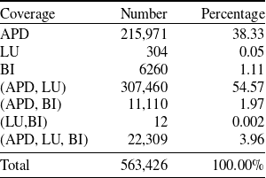
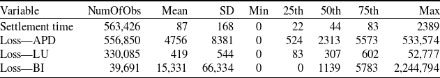
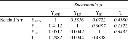
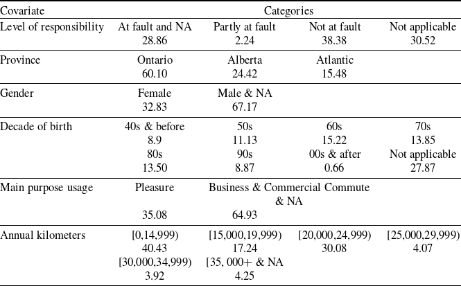
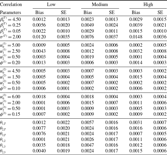
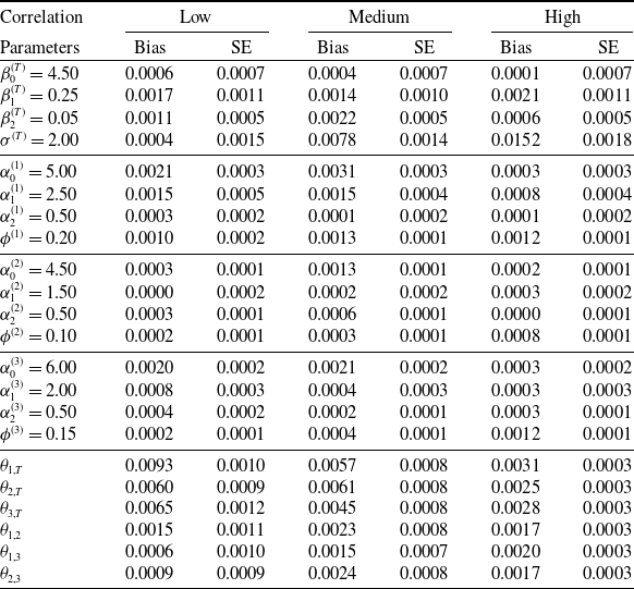


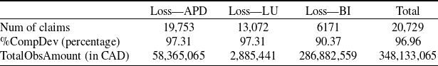
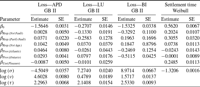
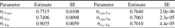
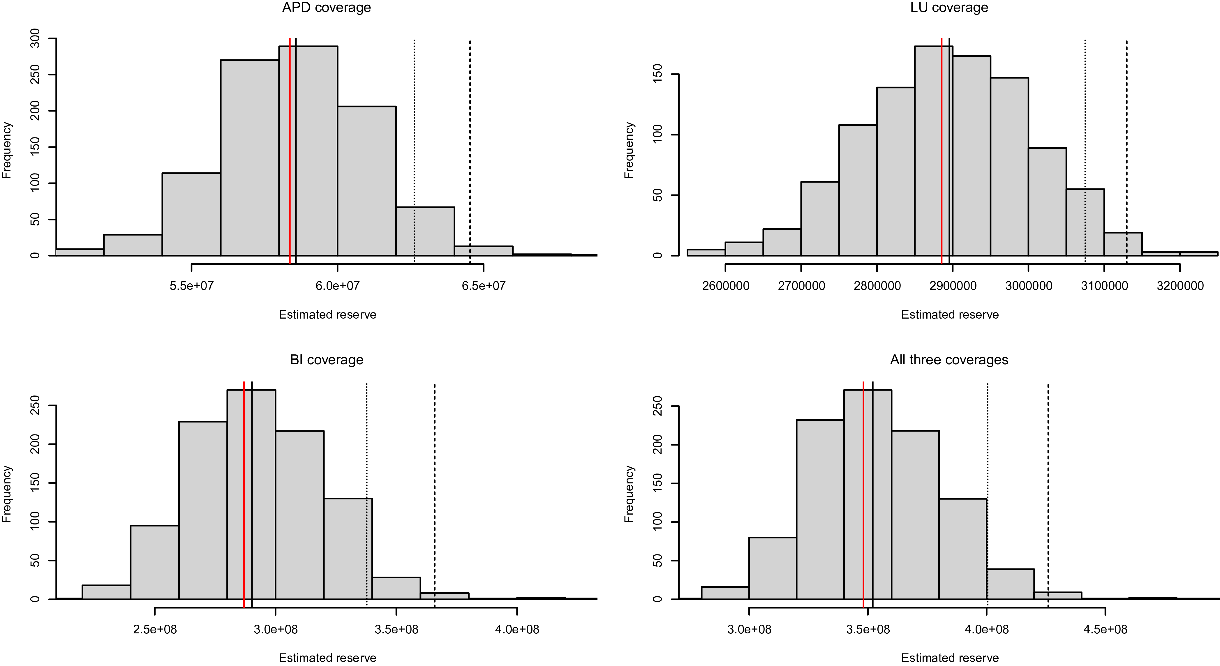
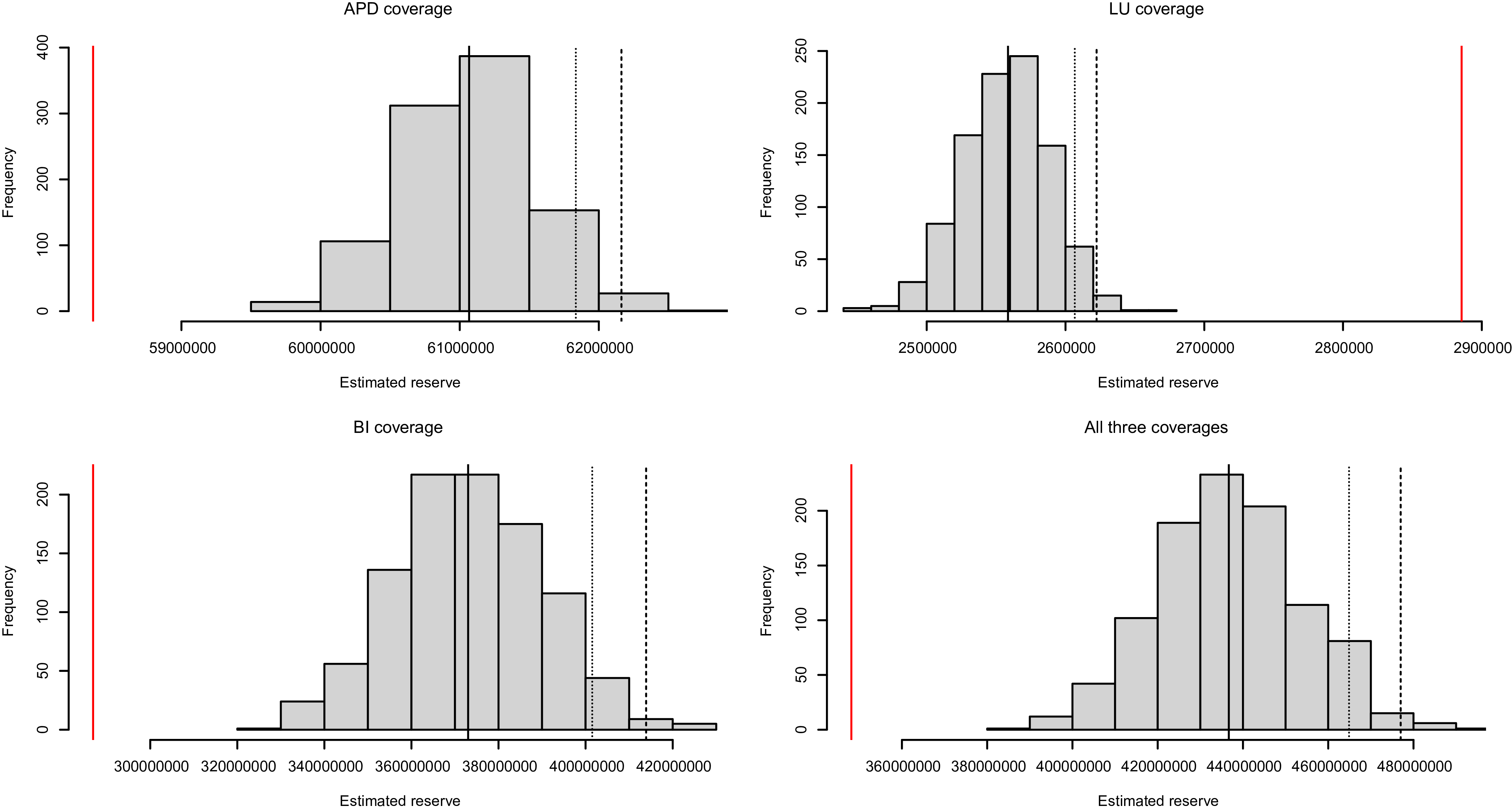
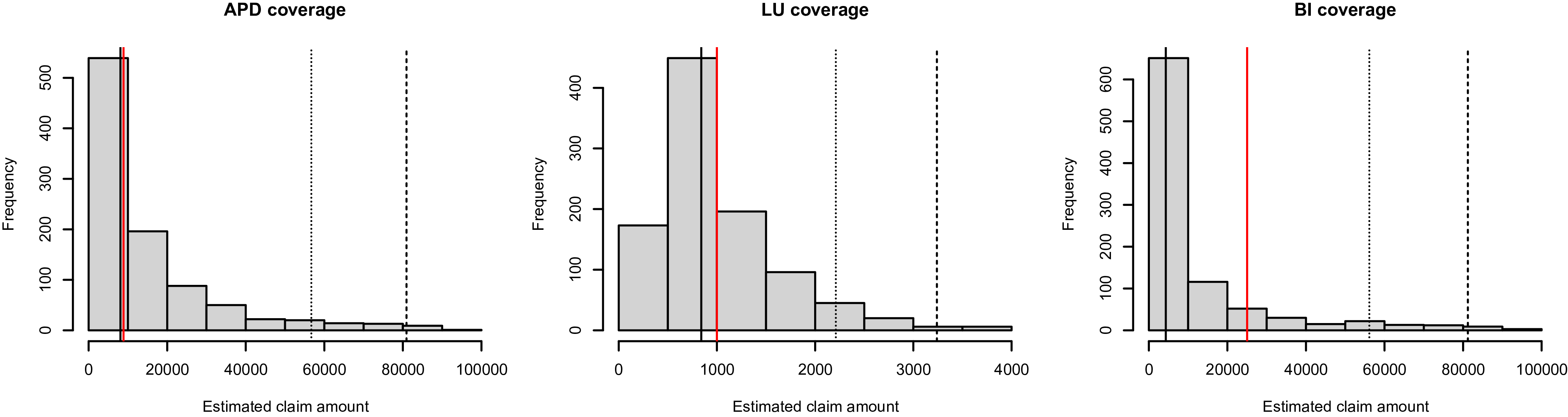
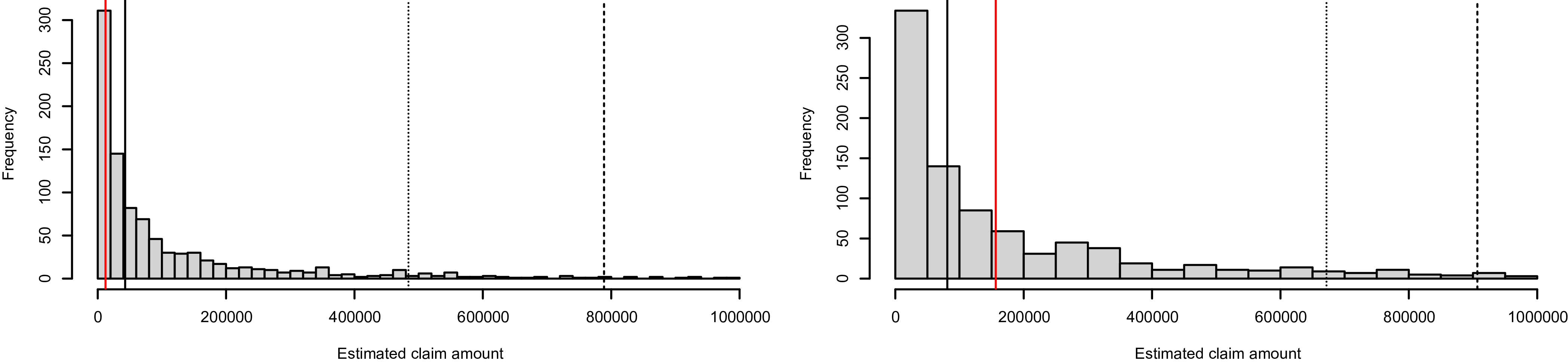


 Open access