

1 Introduction
Many voters and policy analysts perceive increased college completion rates as a high return investment, for both individual students and the United States. However, increased college completion is burdened by rising college costs. These rising costs have sparked questions about whether traditional college financial aid policies – usually targeted on financial need, merit, or both – can increase college completion in a way that is both effective and efficient. Are such policies “effective,” sizably increasing overall college completion rates? Are such policies “efficient,” yielding large increases in college completion relative to costs?
On the one hand, need-based financial aid, such as the federal Pell grant program, targets groups that are underrepresented among college completers. Such aid is complicated to administer at scale, lowering take-up rates and limiting its effectiveness in reaching students. In addition, such aid often goes to students who do not complete college, reducing its efficiency. On the other hand, merit-based financial aid that ignores need is often used by students who would have gone to college anyway (Cornwell & Mustard, Reference Cornwell and Mustard2006, Reference Cornwell and Mustard2007), which limits merit aid’s efficiency and effectiveness in increasing college completion. Targeting both need and merit, by targeting the low-income, academically ready population, is likely efficient, boosting marginal college completion by a large amount relative to costs. But such tightly targeted aid reaches relatively few people, as the population that is both low income and academically ready is small.Footnote 1
Place-based college scholarships can provide empirical evidence on the benefits and costs of different scholarship designs. These scholarship programs, of which several dozen currently exist in the United States, are “place-based” in that the scholarship is based on a high school graduate’s locality – most often the local school district. Although many such programs have merit or need requirements, some do not. In particular, the Kalamazoo Promise scholarship has no achievement or need requirements. Moreover, it pays up to 100% of 4 years of college tuition and is easy to understand and apply for. Therefore, the Kalamazoo Promise represents a good local laboratory for studying the efficiency and effectiveness of proposals calling for more universal access to college aid.
In this paper, we complement our companion paper (Bartik, Hershbein & Lachowska, Reference Bartik, Hershbein and Lachowska2015) by conducting a detailed benefit-cost analysis of the Kalamazoo Promise for different groups of students. In the companion paper, we find that the Promise increases college completion, but heterogeneously by demographic group. In this paper, we incorporate these college completion results into a benefit-cost model that analyzes the benefits and costs of the Promise for groups defined by family income, ethnicity, and gender.Footnote 2 This requires projections by group of earnings effects of a college education, as well as analysis of Promise costs by group. Our analysis shows that the Promise has high benefit-cost ratios and rates of return for both low-income and non-low-income groups, for non-Whites, and for women. Although benefit-cost ratios and rates of return are smaller for men and for Whites, and the weighted average of group-specific rates of return is lower than the simple aggregate rate of return, we conclude that the Kalamazoo Promise easily passes a benefit-cost test. Hence, the lack of targeting of merit or need by the Kalamazoo Promise does not inhibit the program from having high cost-effectiveness. Furthermore, its universality means that by definition the Kalamazoo Promise operates at a large scale, with wide take-up. The Promise’s high returns for both low-income and non-low-income groups suggest that broad-based financial aid programs, under certain conditions, can cost-effectively boost college completion for a wide range of students.
The remainder of this paper is organized as follows. The next section provides background on the Kalamazoo Promise, and reviews its impact on college completion. We then describe how we use these effects and other data to calculate costs and earnings benefits for each subgroup of family income, race, and gender. We consider the sensitivity of these benefit-cost estimates to alternative assumptions. We discuss these results’ implications for proposed scholarship designs. Finally, we conclude by arguing for the importance of disaggregated analysis of the impacts of financial aid programs, as it can lead to surprising conclusions.
2 The impacts of the Kalamazoo Promise on college success
For our benefit-cost analysis of the Kalamazoo Promise, the following features of the Promise are most salient:
-
∙ Generous. The Promise pays for up to 130 credits of college tuition and fees at any public college or university in Michigan.Footnote 3 Footnote 4
-
∙ Universal. The Promise is awarded without academic need or merit requirements.Footnote 5
-
∙ Place-based. The only requirements for Promise award are that the recipient must graduate from Kalamazoo Public Schools (KPS), and must have continuously attended KPS and lived in the district since at least the beginning of 9th grade.Footnote 6
-
∙ Simple. The Promise application is a one-page form in which students provide contact information, their KPS attendance history, and where they will attend college.
-
∙ Mature program. The Promise began with high school graduating class of 2006; thus there is now considerable follow-up data on outcomes.
-
∙ High take-up. Roughly 90% of KPS graduates are eligible for the Promise, and more than 85% of eligibles have received Promise funds. The program’s steady-state spending level on scholarships is roughly $12 million per year, with about 1,400 students receiving scholarships at any one time.
-
∙ Diverse students. Because KPS has considerable numbers of both low-income and middle-income students, and both non-White and White students, Promise outcomes can be estimated for diverse groups.
-
∙ Privately funded. The Promise is funded by anonymous private donors. The donors’ motivation was to not only help students, but to boost Kalamazoo’s economic development by enhancing the quality of the local workforce (Miller-Adams, Reference Miller-Adams2009).
Previous research has found many Promise effects, including: increased KPS enrollment of all ethnic groups (Bartik, Eberts & Huang, Reference Bartik, Eberts and Huang2010; Hershbein, Reference Hershbein2013); improved disciplinary outcomes of high school students and improved high school GPA for African American students (Bartik & Lachowska, Reference Bartik, Lachowska and Polachek2013); increased student applications to more selective state public universities (Andrews, DesJardins & Ranchhod, Reference Andrews, DesJardins and Ranchhod2010). For the current benefit-cost analysis, however, we rely mainly on results from Bartik et al. (Reference Bartik, Hershbein and Lachowska2015) that estimate that the Promise has significantly increased postsecondary credential attainment rates – particularly bachelor’s degree receipt – both overall and among various demographic groups. These estimates rely on a difference-in-differences strategy, comparing eligible to ineligible students, before and after the Promise took effect.Footnote 7
Table 1 summarizes these estimated Promise effects on postsecondary attainment. The overall effects are 12 percentage points on attainment of any credential (degrees or certificate), and 10 percentage points on attainment of a bachelor’s degree. Both effects are about one-third of the pre-Promise mean for a similar population.
Promise effects on degree attainment at 6 years after high school graduation.

Note: Source is Bartik et al. (Reference Bartik, Hershbein and Lachowska2015). (Group-specific results for any credential were not reported in that paper.) Standard errors robust to heteroskedasticity are in parentheses. ***, **, and * indicates $p$
less than 0.01, 0.05, or 0.10. All regressions include controls for graduation year, sex, race/ethnicity, free/reduced-price lunch status, and high school of graduation (except when subgroup is restricted on one of these dimensions); results in panel A also use inverse propensity score reweighting to make post-Promise cohorts resemble pre-Promise cohorts on the same set of observables (estimates without reweighting are similar, but slightly smaller). Income groupings pertain to student eligibility for free/reduced-price lunch. The mean of the dependent variable for each group is calculated over the eligible population in the pre-Promise period. Sample sizes are: overall, 2896; non-low, 1641; low, 1259; White, 1545; non-White, 1360; male, 1388; female, 1517.
$p$
less than 0.01, 0.05, or 0.10. All regressions include controls for graduation year, sex, race/ethnicity, free/reduced-price lunch status, and high school of graduation (except when subgroup is restricted on one of these dimensions); results in panel A also use inverse propensity score reweighting to make post-Promise cohorts resemble pre-Promise cohorts on the same set of observables (estimates without reweighting are similar, but slightly smaller). Income groupings pertain to student eligibility for free/reduced-price lunch. The mean of the dependent variable for each group is calculated over the eligible population in the pre-Promise period. Sample sizes are: overall, 2896; non-low, 1641; low, 1259; White, 1545; non-White, 1360; male, 1388; female, 1517.
These overall effects are larger than found in recent studies of scholarships that are more targeted. For the merit-based West Virginia PROMISE program, Scott-Clayton (Reference Scott-Clayton2011) finds a 4–5 percentage point increase in bachelor’s completion, a little more than 10% of the pretreatment mean. For the need-based Florida Student Access Grant, Castleman and Long (Reference Carneiro and Leeforthcoming) find bachelor’s completion effects of about 4–5 percentage points (22% ).
For the need-based Wisconsin Scholars Grant, Goldrick-Rab et al. (Reference Goldrick-Rab, Kelchen, Harris and Benson2015) find a 4–5 percentage point (29%) increase in bachelor’s attainment.Footnote 8
For the groups, Promise effects show a diverse pattern. Across income background, effects for either completion outcome vary only slightly in magnitude, about 3 percentage points.Footnote 9 Both types of students have effects that are large in both absolute and proportional terms (6 to 12 percentage points, or 22% to 57%).
However, across race and gender, there are larger differences. The Promise has (an imprecisely estimated) null effect on credential completion of White students, but it substantially boosts college completion among students of color, especially in proportional terms (around 50%). Due to smaller sample sizes, we cannot rule out the same treatment effect across ethnic groups at conventional levels of statistical significance. However, because the differences are large in magnitude, and because Bartik et al. (Reference Bartik, Hershbein and Lachowska2015) do find statistically significant differences across ethnicity for other dimensions of postsecondary success (e.g., credit completion after 2 years, for which more cohorts of data are available), we regard the estimates that allow for ethnic differences to be preferable to estimates that do not.
In the case of gender, the differences in estimated effects between men and women are even larger and are statistically significant at conventional levels. While men’s completion appears unaffected by the Promise, women experience very large gains of 13–19 percentage points (45%–49%).
Comparable group-specific estimates in the literature are rare. The need- or merit-based nature of other scholarships can make it difficult to find diverse income groups using the same scholarship, and few other scholarship studies have looked at heterogeneous effects by ethnicity or gender. An exception is Goldrick-Rab et al. (Reference Goldrick-Rab, Kelchen, Harris and Benson2015), who find stronger effects for women than for men but weaker effects for students of color than for Whites.
3 Baseline methodology for comparing benefits versus costs for the Kalamazoo Promise
Our baseline methodology for comparing Promise benefits versus costs is simple. Based on the estimated increase in bachelor’s degrees and associate degrees, we compute the resulting increase in expected lifetime earnings, both overall and for different groups. The present value of these lifetime earnings increases is then compared with the costs of the Promise scholarships.
Such a benefit-cost analysis is incomplete. Focusing on earnings understates benefits because it omits education’s nonpecuniary returns: improved health, reduced crime, and increased civic participation (Currie & Moretti, Reference Currie and Moretti2003; Moretti, Reference Moretti2004; Oreopoulos & Salvanes, Reference Oreopoulos and Salvanes2011). Earnings does not fully capture an individual worker’s change in well-being, as increased earnings come in part from reduced unemployment and increased labor force participation, which may both reduce stigma effects of unemployment and reduce leisure time.Footnote 10 Individual earnings may understate collective earnings increases if there are spillover benefits of some workers’ skills on other workers’ productivity, due, for example, to agglomeration economies (Moretti, Reference Moretti2003, Reference Moretti2004, Reference Moretti2012). Gross earnings increases also have distributional effects, such as increased tax revenues, and reduced transfers, that should be considered in an ideal analysis.
On the cost side, the total financial costs of a scholarship program should include administrative overhead. Scholarships that increase education may come with opportunity costs due to reduced leisure and reduced earnings while in college. In addition, increased educational costs may arise from external subsidy costs to the government if the actual costs of providing additional education exceed tuition. Treating scholarships as a pure cost ignores the benefits of this income transfer for students and their families.
All this being said, a straightforward comparison of earnings benefits with scholarship costs has several virtues: relative ease of estimation; relevance to salient benefits and costs; and comparability with the literature. Earnings benefits and scholarship costs can be measured relatively objectively, whereas estimating other possible benefits and costs (e.g., nonpecuniary benefits/costs of education or work) is more subject to disagreement. In any complete benefit-cost analysis, earnings benefits and scholarship costs would be highly important components. Finally, comparing earnings benefits and scholarships costs is similar to what other researchers have done (e.g., Dynarski, Reference Dynarski2008 and Scott-Clayton, Reference Scott-Clayton2009), which allows results to be compared.
Although our baseline methodology compares only earnings benefits and scholarship costs, later we consider the robustness of our findings to additional benefits and costs.Footnote 11
4 Cost analysis of Promise scholarships
We calculate average scholarship costs per student, in 2012 dollars, and discount costs to the time of high school graduation, both for the overall sample and for the six groups in our educational attainment analysis.
To match the educational estimates presented earlier, we calculate costs for only the first 6 years after high school graduation.Footnote 12 We use cost data for only the 2006 and 2007 graduating cohorts because full cost data are unavailable for the last cohort in the attainment analysis (2008), but as shown below, there is little change over time in costs per student. Otherwise, we include cost data for every student in the educational attainment analysis sample: 388 students from the class of 2006 and 462 students from the class of 2007.Footnote 13
The cost data provided to us by the Kalamazoo Promise report payments per student for three time periods each year: Summer, Fall, and Winter/Spring. We adjust these dollar amounts for inflation by calendar quarter using the personal consumption expenditures (PCE) deflator, and we apply various discount rates, setting $t=0$
to June 15 of students’ graduation year.Footnote
14
$t=0$
to June 15 of students’ graduation year.Footnote
14
Most of the analysis uses a real discount rate of 3%.Footnote 15 However, we also consider the internal rate of return that equates Promise earnings benefits with Promise scholarship costs. We emphasize that our costs per Promise-eligible student include eligible students who never receive Promise funds. This makes our cost estimates comparable with our educational attainment estimates, which include all Promise-eligible students, not just Promise users.
Costs of the Kalamazoo Promise per Promise-eligible student, by subgroup.
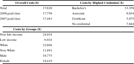
Note: Costs are present discounted values as of high school graduation, using a 3% discount rate and in 2012 dollars, of Kalamazoo Promise scholarship payments made during first 6 years after high school graduation. Costs are per Promise-eligible student. All entries, except for the 2006 and 2007 grad class lines, represent averages for the two graduating classes. Demographic characteristics are from KPS data; highest credential (within 6 years of high school graduation) is from KPS data merged with National Student Clearinghouse data. Low-income students are those who in high school were eligible for a free or reduced-price lunch (family income below 185% of poverty). White students exclude Hispanic students.
Table 2 shows the present value of Promise scholarship costs per student, both overall and by group. The largest source of variation in Promise costs per student is the highest credential attained. Students who earn bachelor’s degrees have higher Promise costs, both because they attend college for more years, and because 4-year colleges are more expensive than 2-year colleges. Students earning a bachelor’s degree have Promise costs more than three times as large as students earning an associate degree.
For more-advantaged groups, Promise costs are higher. Costs per student are over twice as great for non-low-income students ($24,000) as for low-income students ($9,900). Costs are almost twice as great for White non-Hispanics ($22,600) as for other racial groups ($11,900). Costs are only slightly greater for women ($18,400) than for men ($16,800).
5 Constructing earnings profiles to evaluate the Promise’s earnings effects
5.1 Overall logic of earnings benefits computations
To estimate the Promise’s earnings benefits, we first use cross-sectional microdata (described in the next subsection) to compute, both overall and for our six groups, average earnings by age and by three educational categories: individuals with a high school diploma but no higher degree; those with an associate degree; and those with at least a bachelor’s degree. To infer the earnings benefits of obtaining an associate degree due to the Promise, we compute the net present value of having an associate degree relative to a high school diploma and multiply this value by the estimated effect of the Promise on obtaining an associate degree. To infer the earnings benefits of obtaining a bachelor’s degree due to the Promise (including the option value of obtaining a graduate degree), we compute the net present value of having a bachelor’s or higher degree relative to a high school diploma and multiply this value by the estimated effect of the Promise on obtaining a bachelor’s degree. We sum these net present discounted values to obtain the earnings benefits of greater degree attainment due to the Promise.
These calculations rely on two assumptions. First, that cross-sectional variation in earnings by educational attainment can be interpreted as the causal effects of education on earnings. Second, that the marginal student whose education increases because of the Promise will experience the same earnings increase as is true in the cross-section.Footnote 16 For example, perhaps Promise-induced college graduates will be less likely to go on to get graduate degrees than is true in the cross-sectional data.
Much evidence exists on education’s causal relationship to earnings (Card, Reference Card, Ashenfelter and Card1999 and Zimmerman, Reference Zimmerman2014 offer reviews). Causal estimates are similar to cross-sectional differences. In later robustness checks, we adjust estimates to causal effects based on prior research.
As for whether marginal students induced into obtaining more education by the Promise experience average (cross-sectional) returns, the literature is divided. Structural models suggest that returns for marginal students are likely to be lower than observed in cross-sectional data (Willis & Rosen, Reference Willis and Rosen1979; Carneiro & Lee, Reference Carneiro and Lee2004; Carneiro, Heckman & Vytlacil, Reference Carneiro, Heckman and Vytlacil2011). But studies that incorporate credit constraints and other frictions into college selection suggest that marginal returns may be higher (Card, Reference Card2001; Brand & Xie, Reference Brand and Xie2010). While we believe that the assumption of marginal returns equaling average observed returns is reasonable, we explore sensitivity to different education returns in a later section.
5.2 Detailed construction of earnings paths for race, sex, and the overall sample
For the overall sample and the race and gender groups, constructing education-specific career earnings paths is straightforward. As described above, we use cross-sectional variation in earnings by age and education, and then adjust for mortality and secular wage growth.
Our cross-section annual earnings data come from the 2012 American Community Survey (ACS), which provides a large enough sample to estimate average earnings for groups by single year of age. Our annual earnings data reflect only wages and salaries and exclude self-employment income. Observations with imputed earnings are dropped. Observations with zero earnings are included, to reflect both wage and employment rate differences.
Our three education groups are: high school diploma, but no postsecondary degree; associate degree but no higher degree; bachelor’s degree or higher. For each education group, we calculate mean earnings for cells defined by single year of age and demographic group, applying the ACS sample weights. We include ages 25 through 79. Many individuals have not completed schooling before age 25, and our estimated Promise effects are 6 years after high school graduation, when the modal student would be 24. Therefore, it is difficult to know how to treat earnings at younger ages, and so we exclude them.Footnote 17 Earnings after age 79 are assumed negligible.
Next, these cross-sectional earnings profiles are adjusted for secular wage growth. We adopt the assumption of the Social Security Administration (SSA) Board of Trustees of 1.2% annual real wage growth over the next 60 years (Table V.B.1. 2015 OASDI Trustees Report). Our adjustments are for a Promise student graduating in 2006, the first Promise class. A typical student in this class would be 25 in 2013. Earnings at age 25, received in 2013, are increased by 1.2% from the 2012 cross-section estimate for age 25; earnings at age 26, received in 2014, are increased by 2.414% ( $1.012^{2}$
) from the 2012 estimates for age 26; and so on for subsequent ages.
$1.012^{2}$
) from the 2012 estimates for age 26; and so on for subsequent ages.
These wage projections could be biased. SSA may overstate future earnings growth. Earnings in 2012 may be depressed by the Great Recession, which will cause earnings benefits to be understated. Younger cohorts may obtain more postgraduate degrees than past cohorts, with the result that cross-sectional data for older ages will understate education differences in earnings for younger cohorts as they age. The number of persons in prison in different groups may change over time, also altering relative earnings.Footnote 18 The returns to education may be subject to secular changes, up or down. To address these issues, we perform some sensitivity tests later.
We then use the 2010 U.S. Life tables (Arias, Reference Arias2014) to adjust earnings profiles at later ages for expected mortality (by group) since age 18. We use the relevant life tables for the overall population and the race and gender groups.Footnote 19 These Life Tables may also be subject to some bias, as mortality rates will presumably decline over time.
Finally, we apply the same present value discounting as we did with Promise costs.
These calculations suffice for race and gender groups. However, groups defined by family income background require a more complex procedure, described next.
5.3 Calculating expected earnings benefits for low-income students
Calculating future earnings for individuals who grew up eligible for the federal free or reduced-price lunch program is challenging. Cross-sectional data sources, including the ACS, do not measure a person’s family income from years ago.
Therefore, we turn to the Panel Study of Income Dynamics (PSID), which has tracked the same individuals and their descendants since 1968. In the PSID, we can identify whether individuals at ages 13 through 17 lived in families whose income fell below or above 185% of poverty.Footnote 20 As these individuals age, we observe their earnings and education. We calculate average real earnings for each age and education level separately for individuals who grew up in low-income families and those who did not.Footnote 21
The resulting earnings profiles appear in Figures 1(a) and 1(b). Several features are evident. First, as expected, more education is associated with greater earnings, especially with a bachelor’s degree. Second, individuals who grew up in low-income families earn substantially less than those who did not. Third, the disadvantage from a low-income background increases with age. Fourth, the relative disadvantage of growing up low income is larger for individuals with a bachelor’s degree.
(a) Earnings Profiles by Education for Individuals Who Grew Up With Family Incomes Below 185% of the Poverty Line. (b) Earnings Profiles by Education for Individuals Who Grew Up With Family Incomes Above 185% of the Poverty Lines. Source: Authors’ calculations from the PSID. Note: Adjusted to year 2014 dollars using the Personal Consumption Expenditures (PCE) Deflator from the Bureau of Economic Analysis. “Bachelor’s and above” includes respondents who had 16 or more years of education at age 25; “Associate’s degree” includes respondents who had 14 or 15 years of education at age 25; “High school or some college” includes respondents who had 12 or 13 years of education at age 25. Family-income classification is based on average family income when respondent was 13–17. Profiles are fitted values from regressions of annual earnings on a quadratic in potential experience and year-of-observation dummies with the latter netted out.

However, age-earnings profiles may have changed over time from the cohorts in the PSID, making these earnings profiles less representative today. We therefore adjust the PSID profiles to be compatible with the ACS 2012 profiles. We do so by assuming that although absolute earnings may have evolved, the relative earnings of individuals who grew up in low-income families, compared to those who did not, has remained the same. In the PSID, for each specific age and education level, we calculate the ratio of income-background-specific earnings to average earnings (pooled across income backgrounds). We multiply these ratios by the equivalent average overall earnings cell for the respective age and education group in the ACS to yield our calculated earnings stream for individuals from different family income backgrounds.Footnote 22
5.4 Returns to education by group
Before turning to the benefit-cost estimates, we consider what these estimated earnings paths imply for the returns to education by group. Table 3 shows, as one would expect, that there are high earnings returns to increased education, especially for obtaining a bachelor’s degree. The average increase in the present value of earnings from getting a bachelor’s degree, relative to no degree at all, is over 140%. These proportional returns are equally high for most groups, with one notable exception: individuals from a lower income background. For these individuals, the observed bachelor’s premium is just under 70% – half the average.
This surprising new finding, that individuals who come from low-income families have lower returns to education, obviously deserves further investigation (in a separate paper). This disadvantage could be due to unmeasured skills, job networks, college quality, college majors, occupational choice, health, regions, neighborhoods, and other factors. Whatever the causes, these differences in education returns with family background should be reflected in benefit-cost studies of educational investments.
In contrast, different racial groups have similar dollar benefits from educational credentials. Because non-Whites have lower earnings, similar dollar benefits translate to higher percentage benefits. Finally, women and men have similar percentage returns to a bachelor’s degree, but women have lower dollar returns. For associate degrees, women have somewhat higher percentage returns than men, but similar dollar returns.
Projected PDV earnings and returns to education, by group.
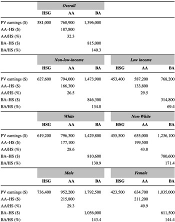
Note: Present value in 2012 dollars, rounded to nearest hundred, is calculated as of age 18 and based on a 3% discount rate. Discounted career earnings cover ages 25–79, adjusted for secular earnings increases and mortality as described in the text. “HSG” includes regular high school diplomas and those with some college but no postsecondary degree. “AA” includes associate degree holders with no higher degree. “BA” includes bachelor’s degree holders and holders of higher degrees.
6 Benefits vs. costs of the Kalamazoo Promise, overall and by group
We combine the estimated returns to education by group (Section 5), and the estimated Promise costs by group (Section 4) to calculate benefit-cost ratios and rates of return. We analyze two scenarios. Scenario 1 assigns group-specific Promise effects on educational attainment (Table 1). Scenario 2 restricts each group to have the same Promise effects, based on Table 1’s overall estimates. Thus, calculated net benefits in scenario 1 account for heterogeneous effects from the intervention, as well as heterogeneity across groups in costs and earnings effects of education. In scenario 2, differences in net benefits reflect variation only from the latter sources of heterogeneity, which are still quite important.
Which scenario is preferable? As discussed above, for the income groups, the Promise effects are clearly quite similar, so scenario 2 is preferable. For the gender groups, group differences are large and statistically significant, so scenario 1 is preferable. For the ethnic groups, we prefer scenario 1, due to the large substantive differences across ethnic groups and evidence of statistically significant differences for other college outcomes, as previously discussed. However, for all these group analyses, we consider both scenarios for completeness.
Table 4 shows how each scenario affects educational attainment for each group.Footnote 23 The preferred Promise effects scenario for each group breakdown is bolded in the table.
Table 5 reports the present value of benefits, the present value of costs, their net difference, and their ratio. The table also reports the “rate of return,” the highest discount rate under which the present value of benefits is equal to or exceeds the present value of costs. Our preferred scenario for each group breakdown is bolded.
Different scenarios for Promise effects on educational attainment by group.

Note: Pre-Promise distributions are based on observed percentages in each education group prior to the Promise (classes of 2003–2005), among students who would have been eligible for the Promise had it existed then. S1 considers a post-Promise scenario that assumes differential Promise effects on education across groups (Table 1, panels B–D). S2 instead imposes the same Promise effect on education across all groups (Table 1, panel A).
Benefit-cost analysis of the Promise, by demographic groups.

Note: The table reports present value of benefits, present value of costs, ratio of present value of benefits to costs, and present value of benefits minus costs. (All present value calculations use a 3% real discount rate.) The rate of return is the maximum discount rate at which the present value of benefits is equal to or exceeds the present value of costs. Scenario 1 assumes the educational attainment effects of the Promise differ by group; Scenario 2 assumes the effects are the same for both groups. Our preferred scenarios are bolded.
For both income groups, under either scenario, the Promise has a high benefit-cost ratio and rate of return. Regardless of family income, students get future earnings benefits that are much higher than scholarship costs. All the benefit-cost ratios exceed 2, the differences between benefits and costs always exceed $10,000 per student, and the real rate of return always exceeds 6%. Results are even stronger under our preferred scenario (same Promise effects for both income groups), with net benefits exceeding $20,000 per student for both groups, benefit-cost ratios greater than 3, and real rates of return exceeding 9%.
However, the benefit-cost picture is less favorable for the low-income group than implied by the aggregate analysis. This is due to the lower returns to education for students from low-income families. As a result, the (weighted) average benefits for both groups combined are lower than the aggregate estimates, though still considerable.Footnote 24
For non-Whites, the Promise has very high benefit-cost ratios and high rates of return. Benefit-cost ratios under either scenario exceed 5-to-1, the rate of return is over 12%, and net-of-costs benefits per student exceed $50,000. These high ratios and rates of return occur for three reasons. First, Promise effects on educational attainment for non-Whites are large. Second, Promise costs for non-Whites are low, because relatively few non-Whites obtain a bachelor’s degree. Third, education returns for non-Whites are high.
For Whites, Promise benefits differ greatly across scenarios. In our preferred scenario, when group effects differ (Scenario 1), educational attainment effects of the Promise are small for Whites. These small education gains translate into small earnings increases, even though Whites have high education returns. On the cost side, because a large share of White students earned a bachelor’s degree even before the Promise, scholarship costs are high, with many scholarships going to Whites who would have completed a bachelor’s degree without the Promise. Promise scholarships may benefit these White graduates by reducing debt burdens, but it does not boost their bachelor degree attainment and thereby earnings.Footnote 25 Consequently, at a discount of 3%, Promise earnings benefits for Whites are less than scholarship costs; the rate of return that equalizes the two is less than 2%.Footnote 26
However, if we restrict the two racial groups to have the same Promise effect (Scenario 2), which cannot be rejected at conventional significance levels, then White results are favorable. Under this scenario, the Promise for White students has a benefit-cost ratio exceeding 3. We do not trust this scenario, as it is inconsistent with evidence suggesting different Promise effects by ethnic group. But regardless of what scenario is believed, the Promise’s high benefits for non-Whites are robust, whereas the benefits for Whites are sensitive to specification.
For women, under either scenario, the Promise has large net benefits. Under our preferred Scenario 1, with different education effects across genders, benefits exceed costs by more than $69,000, which corresponds to a benefit-cost ratio of 4.75 and a rate of return in excess of 12%. For men, under the same scenario, the Promise has no positive earnings benefits: the program does not improve educational attainment for men, and thus provides no earnings increase, but it has large costs because of the high baseline number of men attending college and getting degrees. High returns for men occur if Promise effects across gender are restricted to be the same (Scenario 2); however, this restriction is clearly rejected by our data.Footnote 27
Given these results, it would be of interest to examine Promise effects for narrower subgroups – for example, low-income non-White men. Unfortunately, such finer breakdowns are precluded by our modest sample size.
How do our results compare with previous scholarship studies? Scott-Clayton (Reference Scott-Clayton2009) finds a benefit-cost ratio from the West Virginia merit-based PROMISE scholarship of 1.48, and Dynarski (Reference Dynarski2008) calculates a benefit-cost ratio of about 2 (or an IRR of 7.9%) from the Arkansas and Georgia state merit scholarships. The Kalamazoo Promise’s relatively large returns are due to its larger effects on educational attainment.
7 Sensitivity to alternative calculations of benefits and costs
In this section, we examine how our estimates change by considering additional or alternative costs and benefits and distributional concerns.
7.1 Additional costs
Our baseline costs include only scholarships outlays. Here we add two other types of costs: Promise administration and public subsidies of additional public college attendance.
Administration costs for the Kalamazoo Promise are relatively low: just 3.6% of annual scholarship costs, according to figures provided by the program director.Footnote 28
The actual costs to provide public higher education exceed tuition and fees, as community colleges and universities receive subsidies for instructional purposes from local taxes (community colleges) and state government (community colleges and universities). We estimate these public subsidies using institution-level expenditure and tuition data from the Integrated Postsecondary Education Data System (IPEDS), produced annually by the National Center for Education Statistics. We first compute school-specific subsidies by taking the ratio of academic expenditures per full-time equivalent student and published tuition and fees of institutions attended by Promise recipients.Footnote 29 We then calculate the marginal subsidy costs induced by the Promise by estimating the Promise’s effects on cumulative credits attempted 6 years after high school graduation at Promise-eligible community colleges and Promise-eligible universities, converting these marginal credits into an FTE basis (dividing by 24), and multiplying by a weighted average subsidy rate, where the weights are based on the mix of colleges attended by Promise recipients. We note this approach will tend to overestimate external costs for two reasons: first, it excludes the reduction in subsidy costs from students switching from non-Promise to Promise colleges; second, true marginal external subsidies from additional students attending college are likely less than average costs due to existing fixed costs.
Table 6 shows how the baseline benefit-cost ratios, in our preferred scenarios, are modified by adding these costs.Footnote 30 The benefit-cost ratios only change slightly. Why? First, administrative costs are modest. Second, the public subsidy costs of additional college credits only apply to a portion of Promise recipients, those who increase their college credits.
How benefit-cost ratios change with additional costs added.
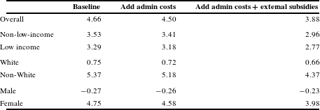
Note: Baseline results for all groups are for preferred scenarios from Table 5.
7.2 Modifying benefit assumptions
This section considers modifications to how recipients’ future earnings are projected, in two ways: using causal education estimates rather than cross-section correlations of education with earnings; and modifying the secular growth assumption. In addition, this section adds in possible spillover benefits of education on others’ earnings.
Our “causal” estimates of education returns are based on two recent studies that have reasonable identification procedures, and are in accord with the research literature: Zimmerman (Reference Zimmerman2014) for bachelor’s degrees and Bahr et al. (Reference Bahr, Dynarski, Jacob, Kreisman, Sosa and Wiederspan2015) for associate degrees. Based on Zimmerman (Reference Zimmerman2014), we scale back our estimated returns to a bachelor’s degree by multiplying our differentials for each group by 93%. Based on Bahr et al. (Reference Bahr, Dynarski, Jacob, Kreisman, Sosa and Wiederspan2015), we rescale our estimates of the return to an associate degree by multiplying our differentials for men by 90.2%, our differentials for women by 129.1%, and our differentials for mixed-gender groups by a weighted average. The appendix available online gives more details on how these specific rescaling percentages were derived. As this above discussion suggests, the available causal estimates do not permit us to have causal adjustments that vary across all six groups in our analysis, as might be ideally desired. Instead, we have to do uniform percentage adjustments, for example for both non-Whites and Whites, or different income groups. Fortunately, the available evidence suggests that adjusting for causation usually does not significantly alter educational returns.
Our baseline estimates assumed a secular real earnings increase of 1.2% annually. As an alternative, this section makes the more pessimistic assumption of zero real earnings growth. Alternatively, this more pessimistic assumption has the same effect as assuming the real dollar value of education returns will stay fixed, even if overall earnings increase. It also is equivalent to scaling back education returns to reflect the possibility that marginal returns may be less than average returns.
As mentioned above, increased education may have social and economic spillover benefits that accrue for others, not just degree recipients. For example, work by Moretti (Reference Moretti2003, Reference Moretti2004) implies that in a local economy, an increase in college completion that directly raises earnings by 1% will raise overall local earnings by close to 2% ; the spillover effect is of similar magnitude to the direct effect. This spillover effect might arise due to skill complementarity through several mechanisms: teamwork effects within a firm, agglomeration economy benefits from a more productive cluster of firms, or innovation spillovers due to skilled workers contributing ideas that boost productivity. We add in spillover benefits of education, using magnitudes from Moretti (Reference Moretti2004).Footnote 31
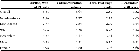
Table 7 reports how our benefit-cost ratios, for different groups, are modified by these changing benefit assumptions. We begin with the final benefit-cost ratios from Table 6, inclusive of additional costs, and then add cumulatively in each benefit assumption.
Despite these different benefit assumptions, the results do not change qualitatively. Benefit-cost ratios still significantly exceed 1 for the overall sample, and for both income groups, non-Whites, and females, while falling short of 1 for Whites and males. The Promise’s educational attainment effects and estimated returns to education are large enough for most groups that scaling back these returns somewhat does not alter results. Furthermore, while adding in spillovers approximately doubles benefit-cost ratios, spillover benefits are not large enough to overcome the small or negative estimated effects of the Promise on the educational attainment of Whites and males.
How benefit-cost ratios change with modified benefit assumptions.
7.3 Distribution of benefits and costs between participants and non-participants
So far, we have quantified various benefits and costs, without focusing on who is affected. This section divides up benefits and costs between Promise participants and nonparticipants. This division helps clarify how the original benefit-cost estimates relate to a more complete benefit-cost analysis.
Participants are simply anyone eligible for the Kalamazoo Promise. Non-participants are all others who might be affected by paying some costs, or receiving some spillover benefits.
We add two key distributional effects. The first effect is cost savings to Promise participants from the tuition scholarships. The second effect is the fiscal benefit to nonparticipants because Promise earnings increases lead to increased taxes and reduced transfers.Footnote 32
The cost savings to Promise participants consist of two components. The first is the cost savings on the tuition they would have paid without the Promise. The second is half of the tuition cost reductions received on any additional Promise-eligible college credits taken.Footnote 33 These two components are calculated from estimates of Promise effects on credits attempted at Promise-eligible 2-year and 4-year colleges.Footnote 34
The fiscal benefits to nonparticipants depend on the marginal tax and transfer rate on increased earnings facing Promise participants. Based on Kotlikoff and Rapson (Reference Kotlikoff and Rapson2007), we assume this rate is 36% .Footnote 35
Table 8 presents this distributional analysis, showing benefits and costs for participants and nonparticipants, which together sum to net social benefits. All benefits and costs are stated on a per-participant basis, in present value 2012 dollars. The benefits of Promise scholarships to participants are counted, which reduces net overall costs of the tuition from a social perspective. Direct earnings are divided into a portion that provides fiscal benefits to nonparticipants, and the remainder which boost the income of participants.
Distributional effects of Kalamazoo Promise, participants vs. non-participants.

Note: All figures are present value from the perspective of an 18-year-old participant in the specified group, using a 3% real discount rate. All values incorporate broader costs and benefits as reflected in the last column of Table 7.
The Promise has sizable distributional effects. Much of the scholarship costs, previously counted only as a cost, reflect a transfer of wealth from nonparticipants to participants. A sizable portion of earnings benefits go to nonparticipants, through increased taxes and reduced transfers. Non-participants also benefit from spillover benefits of more education, while paying greater college subsidy costs.
Overall net benefits of the Promise, counting everyone equally, becomes much more favorable, compared to the baseline of Table 5. Net social costs are lowered by tuition cost savings for participants, and external benefits of education are added in; these two changes outweigh added costs from scholarship administration and public college subsidies.Footnote 36
The original benefit-cost analysis, however, is a rough indicator of the benefits and costs for nonparticipants if it is the case that the sum of the fiscal benefits and external benefits from increased education is of a similar magnitude to the direct gross earnings benefits, which is the case here. We assume fiscal benefits of 36% of direct earnings, and external benefits of 86% of direct earnings, so the benefits to nonparticipants end up being similar to the direct earnings benefits. And because the total costs for nonparticipants are mostly the costs of providing the scholarships, the original benefit-cost picture is a rough guide to the net benefits from the perspective of nonparticipants.
The overall qualitative picture from this more complete benefit-cost analysis – albeit one based on more assumptions – is similar to the original simple comparison of earnings effects with scholarship costs. The Kalamazoo Promise clearly has a large payoff from a variety of perspectives for the overall student body, as well as both income groups, non-Whites, and females. Whether the Promise pays off for White students and male students is more questionable, and depends on how one weights benefits for participants versus nonparticipants.
7.4 Local benefits of the Kalamazoo Promise
As discussed above, the Kalamazoo Promise is funded by anonymous donors, in part to promote local economic development. What local development effects are plausible?
One development effect occurs because of how the Promise affects the Kalamazoo area’s future workforce, due to effects on Promise students. As college graduates are more likely to participate in national job markets, the proportion of college graduates staying in their metro area of origin is less than for noncollege graduates, by about 20 percentage points (Bartik, Reference Bartik2009). Therefore, the Kalamazoo Promise’s college graduation effects would be expected to reduce the probability that local students remain in the area. However, attending college in one’s home state increases the share of college attendees that remain in the state by roughly 10 percentage points (Groen, Reference Groen2004). Because the Kalamazoo Promise successfully encourages students to attend college in Michigan rather than elsewhere, a greater share of Kalamazoo students would be expected to remain in Michigan, and some of these will stay in the Kalamazoo area. In addition, based on observed migration behavior, the historical proportion of college graduates from the Kalamazoo area who remain there for most of their career is approximately 35–45% (Bartik, Reference Bartik2009). Thus, it seems likely that the Promise will result in a sizable proportion of graduates staying in the local area.
Consequently, the long-run net effect of the Promise on the local workforce is that more of Kalamazoo’s children will leave the area, but a higher proportion of those who stay or return will be college graduates. The Promise’s direct effect will be to reduce the local workforce, but improve its quality. This improved quality of the local workforce will increase average local wages, both directly, and through spillover benefits (Moretti, Reference Moretti2004). Some of these spillover benefits will occur because a more skilled workforce will attract more and better jobs to the Kalamazoo area, which in turn will have effects in attracting additional population.
A second local development effect of the Kalamazoo Promise arises from the possibility of more immediate migration effects, due to parents being attracted (or induced to stay) by the scholarships. Earlier research has shown that the Kalamazoo Promise increased the school district’s enrollment by about 30% compared to what it otherwise would be (Bartik et al., Reference Bartik, Eberts and Huang2010), with about one-quarter of this increased enrollment from outside the state (Hershbein, Reference Hershbein2013). Although no detectable impact of the Promise on housing prices has been found in Kalamazoo, broader studies of Promise-style programs have found them to increase housing prices by 6–12% (LeGower & Walsh, Reference LeGower and Walsh2014) and to reduce out-migration so as to increase a local area’s population by about 1.7% within a few years (Bartik & Sotherland, Reference Bartik and Sotherland2016). Simulations by Hershbein (Reference Hershbein2013) suggest that the immediate migration effects of the Kalamazoo Promise might be sufficient to raise gross regional product by 0.7%
In sum, the current evidence suggests that a considerable portion – but by no means all – of the Kalamazoo Promise’s benefits will be captured in some form by the local area. Future empirical work may allow more exact quantification of these geographic distributional effects.
Because local areas do not capture all benefits and costs, an optimal public finance argument can be made that such scholarship programs might be better run at a state or national level. However, this omits possible advantages from greater local flexibility and creativity, which might be realized as areas compete to provide better scholarship programs. For example, the large benefits of the Kalamazoo Promise might stem in part from its simplicity. Such simplicity might be more likely in scholarships that are locally run, compared to scholarships designed by a federal bureaucracy.
8 Conclusion
We find that the Kalamazoo Promise has high benefit-to-cost ratios and rates of return for different income groups, for non-Whites, and for women, and these effects are robust to reasonable alternative assumptions. Whether the Promise has net benefits for Whites and for men is more sensitive to assumptions.
What implications does this have for policy debates on the relative merits of universal and targeted scholarships? Aside from the legal and ethical difficulties in trying to explicitly target a Promise-style scholarship based on race or gender, we note that the Promise effects we have estimated are for a program that is not targeted by group. The lack of group targeting makes the Kalamazoo program simpler and easier to explain, and probably elicits greater public support. These factors likely play some role in the program’s effects.
Our findings might be used to rationalize scholarship programs that are “universal” in that they target all students in a school district, but “targeted” on school districts that have a high percentage of non-White or low-income students. Such districts will have more modest scholarship costs per student because of low baseline rates of college attendance and persistence. Yet, particularly for non-White students, the expected earnings return to increasing educational attainment is quite high.
Our results also point to the importance of disaggregating analyses of educational policies by socioeconomic or demographic group. The rates of return to educational interventions can vary greatly by group, sometimes in surprising ways. For example, differences between disadvantaged and advantaged income groups may not carry over to differences between disadvantaged and advantaged racial groups. Furthermore, because aggregate earnings measures may contain a different composition of groups than the sample populations of education policy interventions, their use can lead to biased benefit-cost ratios when there are heterogeneous treatment effects or heterogeneous returns to education.Footnote 37
Overall, our benefit-cost analysis suggests that the Kalamazoo Promise has high benefits relative to costs. Even with a benefit measure that omits spillover benefits of education, and a cost measure that ignores how scholarships help reduce student and family debt, we find that the universal college scholarship of the Promise, for a wide variety of groups, easily passes a benefit-cost test. When such additional benefits are included, the Promise has even larger net benefits.
These large net benefits of the Kalamazoo Promise, with some striking differences across ethnic groups and gender groups, deserve further examination. The large net benefits of the Promise stem mostly from its sizable effects on college completion, which are larger than those from other scholarships programs that have been studied. Are the Promise’s relatively large completion effects and expected net benefits due to its universal and simple nature? Such a hypothesis is plausible, but should be further examined by looking at the effects of other place-based scholarships, ideally of different designs and in different local contexts.
The much stronger results for women than for men, and for non-Whites than for Whites, also should be explored. Such exploration could be done in part by analyzing other Promise-style programs to see whether they follow similar patterns. In addition, as additional data are collected on the Kalamazoo Promise, larger sample sizes may permit precise examination of Promise effects for smaller subgroups, such as non-White men, White women, or low-income men, which may help further clarify who does and who does not benefit from the scholarship. Finally, the Kalamazoo Promise program itself has ongoing efforts to increase the success rate of all Promise-eligible students. Qualitative or quantitative evaluation of these efforts to help improve the Promise success rate might indicate what, in addition to financial scholarships, is needed to effectively and efficiently improve American college completion rates.
Supplementary material
To view supplementary material for this article, please visit https://doi.org/10.1017/bca.2016.22.
Acknowledgments
We thank Bob Jorth of the Kalamazoo Promise, Michael Rice of Kalamazoo Public Schools, and Carol Heeter of Kalamazoo Valley Community College for assistance and providing data. We also thank the William T. Grant Foundation for its generous support and Lumina Foundation for its support of the Promise Research Consortium. Stephen Biddle and Wei-Jang Huang provided valuable research assistance on the original analysis of the Kalamazoo Promise, and Wei-Jang Huang assisted with the PSID data. The authors have no material interests or current affiliation with the Kalamazoo Promise or Kalamazoo Public Schools; Bartik previously served on the Kalamazoo Public Schools Board between 2000 and 2008. All errors are our own.


 Open access