





1. Introduction
Alpine glaciers are widely recognized as sensitive indicators of atmospheric change because their seasonal accumulation and ablation respond directly to long-term changes in air temperature and precipitation anomalies (Winkler and others, Reference Winkler, Chinn, Gärtner-roer, Nussbaumer, Zemp and Zumbühl2010; Bliss and others, Reference Bliss, Hock and Radic2014; Huss and Hock, Reference Huss and Hock2018). Over recent decades, glacier mass loss has accelerated across nearly all mountain regions worldwide, including the western North America (Frans and others, Reference Frans, Istanbulluoglu, Lettenmaier, Fountain and Riedel2018; O’Neel and others, Reference O’Neel2019; Menounos and others, Reference Menounos, Huss, Marshall, Ednie, Florentine and Hartl2025), the European Alps (Fischer and others, Reference Fischer, Huss and Hoelzle2015; Huss and Fischer, Reference Huss and Fischer2016; Di Mauro and Fugazza, Reference Di Mauro and Fugazza2022), the Andes (Vuille and others, Reference Vuille2008; Cullen and others, Reference Cullen, Sirguey, Mölg, Kaser, Winkler and Fitzsimons2013; Purdie, Reference Purdie2013; Sagredo and Lowell, Reference Sagredo and Lowell2012), High Mountain Asia (HMA; Lutz and others, Reference Lutz, Immerzeel, Shrestha and Bierkens2014; Gao and others, Reference Gao, Li, Duan, Ren, Meng and Pan2018; Miles and others, Reference Miles, McCarthy, Dehecq, Kneib, Fugger and Pellicciotti2021) and other alpine mountain ranges (Chinn and others, Reference Chinn, Winkler, Salinger and Haakensen2005; Stokes and others, Reference Stokes, Popovnin, Aleynikov, Gurney and Shahgedanova2007; Cullen and others, Reference Cullen, Sirguey, Mölg, Kaser, Winkler and Fitzsimons2013; Purdie, Reference Purdie2013). The accelerated loss of glacier mass impacts downstream hydrology, as fluctuations in meltwater volume influence streamflow patterns and water availability (Carey and others, Reference Carey, Molden, Rasmussen, Jackson, Nolin and Mark2017; Milner and others, Reference Milner2017; Frans and others, Reference Frans, Istanbulluoglu, Lettenmaier, Fountain and Riedel2018; Brighenti and others, Reference Brighenti, Tolotti, Bruno, Wharton, Pusch and Bertoldi2019; Schaefli and others, Reference Schaefli, Manso, Fischer, Huss and Farinotti2019). Therefore, improving our ability to estimate glacier mass balance (MB) in response to climate change is essential for assessing environmental impacts at both local and global scales.
Direct energy-balance and MB observations from stake networks and automatic weather stations offer physically rigorous benchmarks for individual glaciers (Braithwaite, Reference Braithwaite1995; Hock and Noetzli, Reference Hock and Noetzli1997; Arendt and Sharp, Reference Arendt and Sharp1999; Greuell and Smeets, Reference Greuell and Smeets2001; O’Neel, Reference O’Neel2019). However, the labor-intensive logistics of long-term field campaigns limit their spatial coverage. By contrast, satellite remote sensing delivers repeat observations that can be scaled to entire mountainous regions or even to global glacier inventories (Hall and others, Reference Hall, Chang and Siddalingaiah1988; Hall and others, Reference Hall, Riggs and Salomonson1995; Gao and Liu, Reference Gao and Liu2001). Satellite-based optical observations provide critical insights into glacier-surface changes, including surface area loss (Paul and others, Reference Paul2015), velocity fluctuations (Ahn and Howat, Reference Ahn and Howat2011; Fahnestock and others, Reference Fahnestock, Scambos, Moon, Gardner, Haran and Klinger2016) and variations in surface albedo (Wiscombe and Warren, Reference Wiscombe and Warren1980; Konig and others, Reference Konig, Winther and Isaksson2001). Although these satellite imagery observations do not measure mass fluxes directly, they are closely related to surface energy-balance (SEB) processes that govern annual MB and therefore provide a valuable basis for regional upscaling.
Among satellite-derived metrics regarding glacier changes, surface albedo has become a key measure because it links directly to the fraction of incoming shortwave radiation absorbed at the glacier surface and, in turn, to glacier annual MB (Tait, Reference Tait1873; Ångström, Reference Ångström1918; Hock, Reference Hock2005). Observational and modeling studies spanning more than a century have consistently shown that brighter (high-albedo) ice melts more slowly, while darker ice absorbs more energy and melts faster (Hall and others, Reference Hall, Chang, Foster, Benson and Kovalick1989; Oerlemans and Knap, Reference Oerlemans and Knap1998; Arendt and Sharp, Reference Arendt and Sharp1999; Oerlemans and Klok, Reference Oerlemans and Klok2002; Favier and others, Reference Favier, Wagnon and Ribstein2004). The launch of NASA’s Moderate Resolution Imaging Spectroradiometer (MODIS) sensor in 1999 produced the first near-daily global albedo map, but its coarse pixel size and frequent cloud contamination in mountainous regions have limited the use of MODIS for alpine glaciers (Hall and others, Reference Hall, Riggs, Salomonson, DiGirolamo and Bayr2002; Klein and Stroeve, Reference Klein and Stroeve2002). Recent studies have improved MODIS albedo for glacier work by adding cloud masks, filtering steep view angles and filling gaps in space and time (Xin and Sheng, Reference Xin and Sheng2024; Ye and others, Reference Ye, Cheng, Hao, Hu and Liang2024).
With consistent measurements of glacier-surface albedo through satellite remote sensing, researchers have found a strong correlation between satellite-derived albedo and annual glacier melt. For example, Dumont and others (Reference Dumont2012) and Davaze and others (Reference Davaze2018) found significant relationships between minimum summer albedo and annual MB in the European Alps, while Sirguey and others (Reference Sirguey, Still, Cullen, Dumont, Arnaud and Conway2016) reported similarly robust results in New Zealand. Di Mauro and Fugazza (Reference Di Mauro and Fugazza2022) extended this work by testing multiple albedo-based phenology metrics across 31 Alpine glaciers, finding per-glacier R 2 values ranging from 0.27 to 0.83. Ye and others (Reference Ye, Cheng, Hao, Hu and Liang2024) further showed that the observation time series interpolation method matters: raw summer-averaged albedo best predicted MB in Austria (mean R 2 = 0.83), whereas interpolated albedo was most effective in Norway (mean R 2 = 0.81). Complementing these empirical albedo–MB relationships, Phelps and others (Reference Phelps, Radić and Williamson2025) showed across 23 Canadian glaciers that incorporating calibrated remote-sensing-informed albedo corrections into a regional SEB model substantially improved MB simulations, bringing SEB performance to parity with or slightly better than a calibrated positive degree-day model. Together, these findings confirm albedo’s role as a physically grounded and scalable indicator for glacier MB estimation.
Recent research suggests that phenological metrics derived from MODIS temperature–albedo ratio (TAR) time series may offer a more robust method for estimating glacier MB by better capturing seasonal energy dynamics (Xin and Sheng, Reference Xin and Sheng2025). TAR is a composite remote-sensing metric defined from glacier-surface temperature and albedo, intended to characterize surface conditions relevant to melt by jointly reflecting thermal forcing and shortwave energy absorption. Specifically, cumulative melting index (CMI) is calculated by first constructing a TAR time series from MODIS land surface temperature (LST) and albedo observations for each glacier, where LST serves as a proxy for the glacier’s thermal state and atmospheric heat input, and albedo modulates the fraction of incoming shortwave radiation absorbed at the surface. Next, the TAR series is integrated over an adaptive ablation season defined from 100 days before to 30 days after the annual peak TAR date, so that CMI represents the cumulative surface conditions during the main melt season. Annual CMI has shown strong correlations with observed annual MB across a wide range of alpine glaciers globally (Xin and Sheng, Reference Xin and Sheng2025). However, despite these strong correlations, the CMI–MB linear relationship varies substantially among glaciers. Specifically, glaciers in maritime regions, such as southern Norway and the northwestern USA, tend to exhibit steeper slopes than continental glaciers in HMA. This variability suggests that, although glacier-specific factors such as elevation and aspect may influence individual CMI sensitivity, the broader regional variability in the CMI–MB relationship is strongly modulated by climatic setting.
This interpretation is consistent with a large body of glaciological literature showing that glacier MB is governed by multiple interacting climatic controls and that these controls vary systematically across regions. Statistical and process-based studies have long shown that annual MB can often be explained by combinations of temperature and precipitation, with relative sensitivity depending on glacier setting (Lliboutry, Reference Lliboutry1974; Oerlemans and Reichert, Reference Oerlemans and Reichert2000; Marzeion and others, Reference Marzeion, Hofer, Jarosch, Kaser and Mölg2012; Trachsel and Nesje, Reference Trachsel and Nesje2015). Other studies have used multivariate or circulation-based approaches to demonstrate that regional MB variability reflects broader atmospheric controls, including maritime versus continental influence, large-scale circulation anomalies and shifts in accumulation seasonality (Lewis and Smith, Reference Lewis and Smith2004; Christian and others, Reference Christian, Siler, Koutnik and Roe2016; Zhan and others, Reference Zhan, Shi, Wang and Yao2017; Bonan and others, Reference Bonan, Christian and Christianson2019; Zhu and others, Reference Zhu, Thompson, Zhao, Yao, Yang and Jin2021). At mountain-range scales, glacier geometry and topographic setting also modulate climatic sensitivity and complicate extrapolation from observed glaciers to unmeasured populations (Huss, Reference Huss2012). Therefore, the key question is whether glaciers with regionally distinct CMI–mass-balance relationships can be grouped in a way that makes those relationships more comparable and transferable across different climatic settings.
In this study, our aim is not only to evaluate glacier-to-glacier variability in the CMI–MB relationship but also to test whether part of that variability can be understood using a small set of climatic descriptors. By combining remote-sensing phenology metrics with multivariate climate classification, we aim to assess whether climate-informed grouping improves the interpretability and transferability of CMI-based MB estimation across diverse glacier environments. Specifically, we seek to:
1. test whether CMI standardization improves cross-glacier comparability of the CMI–MB relationship;
2. examine the climatic and glaciological controls associated with the residual variability in CMI–MB slopes among glaciers;
3. evaluate the potential of this framework for regional glacier MB estimation from remotely sensed time series; and
4. demonstrate the regional application of this framework through a case study of glacier mass loss in the European Alps.
2. Data
This study uses glacier phenology metrics and associated MODIS-derived TAR time series as described by Xin and Sheng (Reference Xin and Sheng2025). TAR is computed as the ratio of MODIS LST, obtained from the MOD11A1.061 product, to surface albedo, derived from the MOD10A1.061 product. This ratio combines remotely sensed information on glacier-surface thermal state and reflectivity, therefore serves as an empirical proxy for melt-favorable surface conditions. From daily TAR time series, we compute CMI, which is defined as the integral of TAR over an adaptive ablation season centered on the annual peak TAR date. Specifically, the integration window begins 100 days before the annual peak TAR date and ends 30 days after it. This asymmetric window was chosen to capture the typical seasonal evolution of glacier melt, including the rapid intensification of melt leading up to peak surface exposure and the more prolonged decay of ablation conditions afterward. CMI approximates the cumulative energy input to the glacier surface during the ablation season. For additional methodological details, we refer readers to the original formulation by Xin and Sheng (Reference Xin and Sheng2025).
Annual glacier MB data were acquired from the World Glacier Monitoring Service (WGMS) Fluctuations of Glaciers dataset (WGMS, 2024). We selected glaciers that meet the following criteria:
• Have at least 10 years of MB records between 2002 and 2021, and
• Exhibit a significant CMI–MB relationship (i.e. R 2 > 0.5).
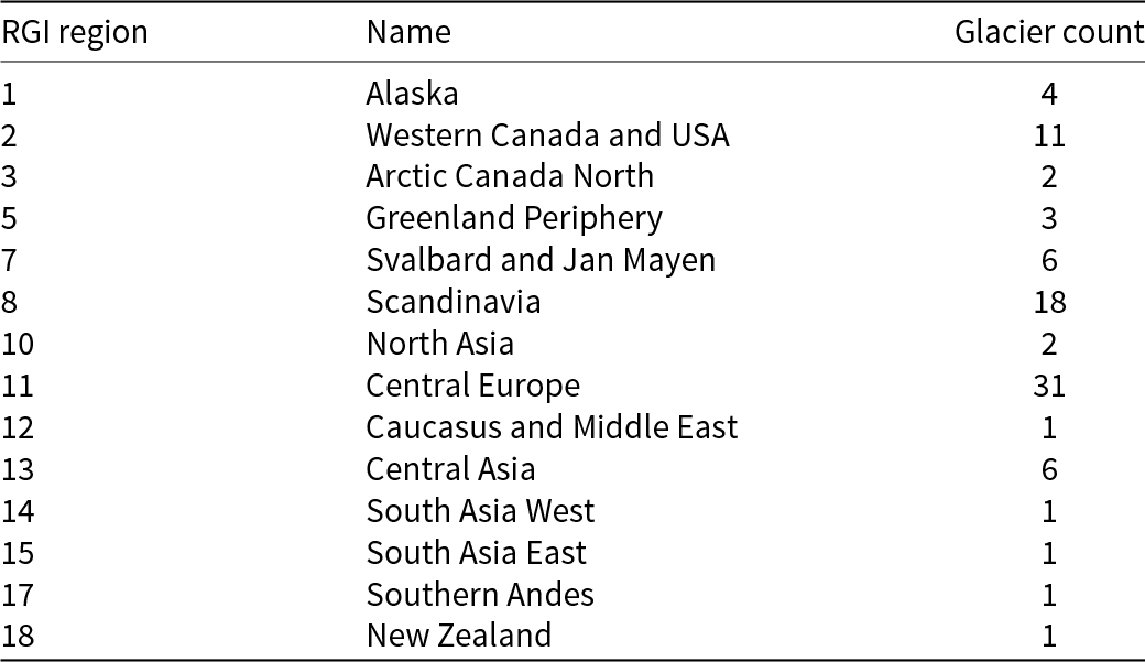
Glacier screening is used here to define the subset of glaciers for which the interannual CMI–MB relationship is sufficiently robust for comparative slope analysis and regional regression transfer; weaker-fit glaciers were examined in our previous work (Xin and Sheng, Reference Xin and Sheng2025), where reduced performance was linked to weak seasonality, debris cover, terrain shadow and mixed-pixel effects. After screening, 88 glaciers were retained for analysis. Table 1 summarizes the distribution of these glaciers by Randolph Glacier Inventory (RGI) regions (RGI 7.0 Consortium, 2023).
Number of glaciers included in this study, grouped by Randolph Glacier Inventory (RGI 7.0 Consortium, 2023) regions (total = 88).

Table 1 Long description
The table lists how many glaciers from the study come from each Randolph Glacier Inventory region, totaling 88 glaciers. Central Europe contributes the largest share with 31 glaciers. Scandinavia is next with 18, followed by Western Canada and USA with 11. Mid-range counts include Svalbard and Jan Mayen with 6 and Central Asia with 6, while Alaska has 4 and Greenland Periphery has 3. Arctic Canada North and North Asia each have 2. Several regions contribute only 1 glacier each: Caucasus and Middle East, South Asia West, South Asia East, Southern Andes, and New Zealand. The counts reflect the study sample by region and do not necessarily represent overall glacier abundance in those regions.
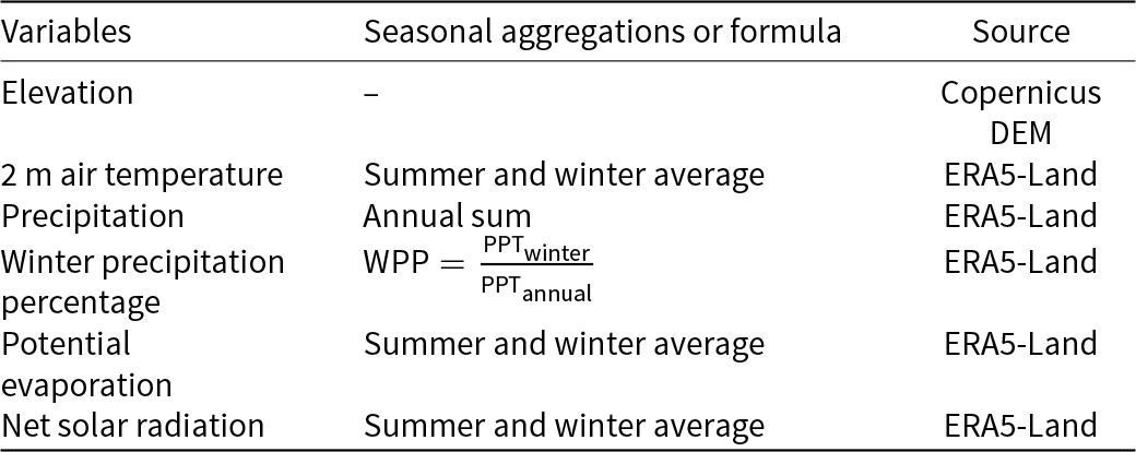
To investigate the impacts of regional climate and topographic conditions on the CMI–MB relationship, we incorporate several explanatory variables into the analysis. Climate variables are derived from the ERA5-Land monthly averaged reanalysis dataset (Muñoz-Sabater, Reference Muñoz-Sabater2019; Muñoz-Sabater and others, Reference Muñoz-Sabater2021). Seasonal means were calculated for a winter half-year (October of the previous year through March) and a summer half-year (April through September) for Northern Hemisphere glaciers. This seasonal division was used to derive predictors describing the seasonal distribution of temperature and precipitation, rather than to define maritime or continental conditions directly. To characterize precipitation seasonality, we computed the winter precipitation percentage (WPP), defined as the ratio of total winter precipitation to total annual precipitation. We used WPP as a glaciologically relevant proxy for the seasonal concentration of snow accumulation. ERA5-Land 2 m air temperature was used directly at the native grid-cell elevation and was not adjusted to glacier median elevation. We acknowledge that this introduces some mismatch between reanalysis elevation and glacier elevation, but in this study temperature variables are used as broad climatic descriptors rather than as glacier-surface energy inputs. Topographic data are derived from the Copernicus Digital Elevation Model (European Space Agency, 2024), using the glacier boundaries provided by the RGI to calculate glacier median elevation. A summary of all climate and topographic variables used in the analysis is provided in Table 2.
Climate and topographic variables used to characterize glacier environmental conditions.

Table 2 Long description
The table defines climate and terrain variables used to describe glacier environmental conditions, along with how each variable is aggregated and where it comes from. Elevation is taken from the Copernicus digital elevation model. Air temperature, potential evaporation, and net solar radiation are summarized as separate summer and winter averages and are sourced from ERA5-Land. Precipitation is summarized as an annual total from ERA5-Land. Winter precipitation percentage is defined as the share of annual precipitation that falls in winter, also from ERA5-Land. A key caveat is that the listed air temperature is a regional near-surface value and is not adjusted to match glacier elevation.
Note: Seasonal means are calculated for summer (Apr–Sept) and winter (Oct–Mar). ERA5 2 m air temperature was used as a regional climate descriptor and was not lapse-rate adjusted to glacier elevation.
3. Methods
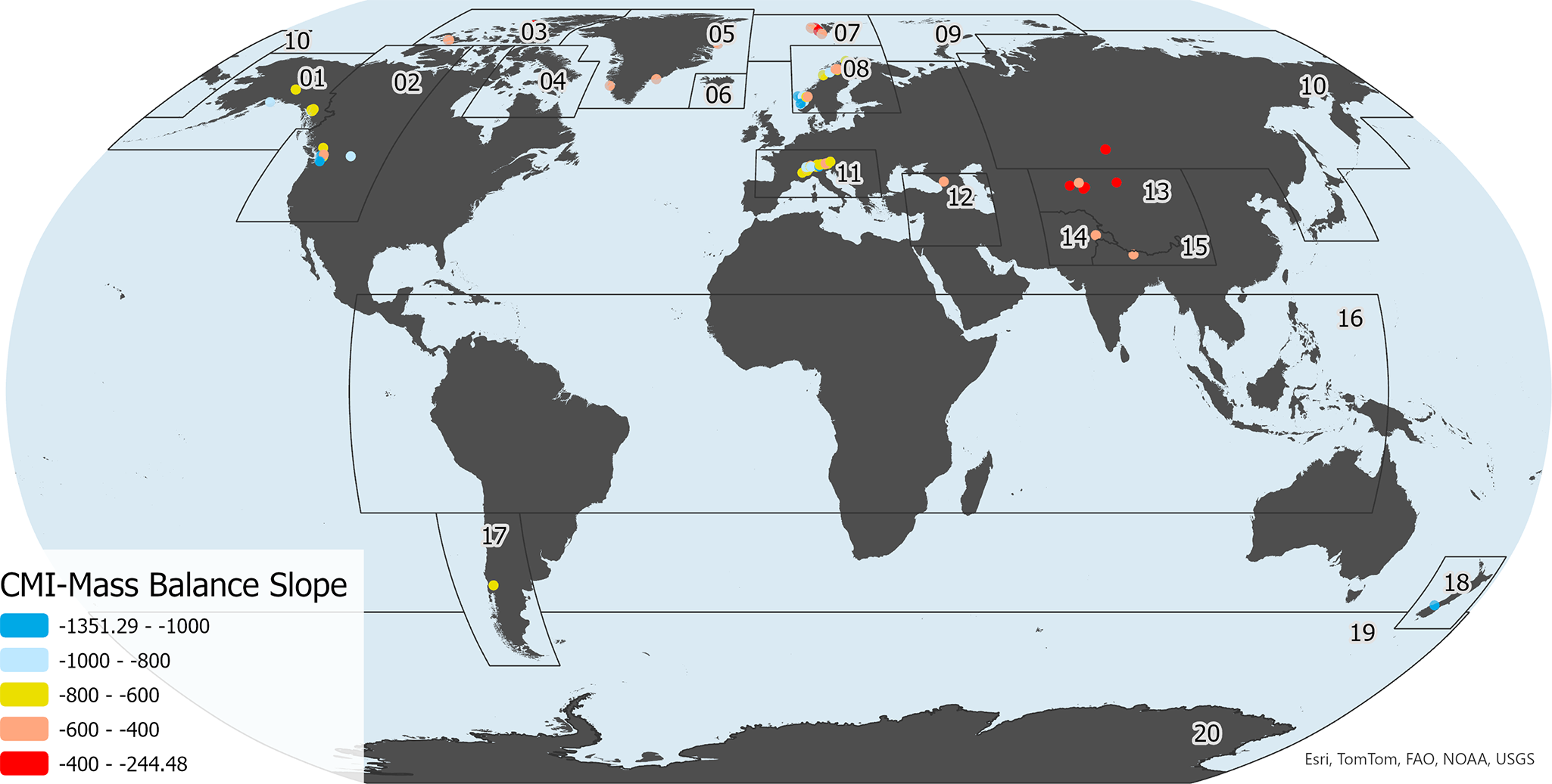
For each glacier, while CMI and annual MB exhibit a strong linear relationship, the slope of this relationship represents the rate of change in MB per unit change in CMI. Because this study focuses on comparing the CMI–MB relationship among glaciers, we standardized annual CMI separately for each glacier by subtracting the glacier-specific mean and dividing by the glacier-specific interannual standard deviation (SD). This transformation does not alter the within-glacier correlation structure but rescales CMI anomalies into units of each glacier’s own year-to-year variability. The resulting regression slope is therefore interpreted as the change in annual MB associated with a 1 SD anomaly in CMI for that glacier. We use this standardized slope for interglacier comparison because slopes derived from raw CMI are partly determined by glacier-specific differences in the variance of CMI and are therefore less directly comparable across contrasting glacier environments. The resulting standardized slopes, hereafter referred to as the CMI–MB slope, are shown in Fig. 1. Glaciers at higher latitudes (e.g. RGI Regions 2 and 8) show more comparable slopes to those in mid-latitude regions, while coastal glaciers exhibit the most negative slopes.
Slopes of the linear relationship between annual glacier mass balance and standardized CMI for the 88 glaciers included in this study. Maritime glaciers exhibit the steepest slopes.

Figure 1 Long description
A thematic world map with north at the top. Land areas are shown with numbered glacier regions and colored point markers. The title reads “CMI-Mass Balance Slope”. Legend categories (CMI-Mass Balance Slope): - minus 1351.29 to minus 1000 - minus 1000 to minus 800 - minus 800 to minus 600 - minus 600 to minus 400 - minus 400 to minus 244.48 Numbered regions and marker placement: - 01: Marker in the far northwest of North America. - 02: Marker in the northeast of North America. - 03: Marker near the North Atlantic between northeastern North America and northern Europe. - 04: Marker in northern Europe. - 05: Marker in far northern Asia. - 06: Marker in western Europe. - 07: Marker in central Europe. - 08: Marker in northern Europe. - 09: Marker in northern Asia. - 10: Marker in central Asia. - 11: Marker in central Asia. - 12: Marker in central Asia. - 13: Marker in central Asia. - 14: Marker in South Asia. - 15: Marker in East Asia. - 16: Marker in Southeast Asia. - 17: Marker along the western side of southern South America. - 18: Marker in the southwest Pacific near an island chain. - 19: Marker in the southern ocean area south of the Pacific. - 20: Marker in the Antarctic region. Overall distribution by legend category: - The most negative category (minus 1351.29 to minus 1000) appears at least once in the far northwest of North America. - Mid-range categories (minus 1000 to minus 800, minus 800 to minus 600 and minus 600 to minus 400) appear across multiple numbered regions in Europe and across central to eastern Asia. - The least negative category (minus 400 to minus 244.48) appears in several regions, including parts of Europe and parts of Asia. Map labels and credits: - Region numbers shown on the map include 01 through 20. - A small credit line appears at the lower right.
As illustrated in Fig. 1, CMI–MB slopes display clear spatial clustering. To better understand this spatial distribution pattern, we applied PCA to the set of seasonal climate variables derived from ERA5. PCA helps reveal underlying patterns in climate and enhances the identification of glacier groups with similar characteristics (Abdi and Williams, Reference Abdi and Williams2010). Nine variables were selected to represent the main climatic controls on glacier dynamics (Table 2). These include seasonal averages of temperature, potential evapotranspiration and net solar radiation to describe thermal and radiative conditions, together with elevation. To characterize moisture regime, we used WPP instead of raw seasonal precipitation totals, as this metrics better captures the distinction between maritime and continental glacier climates. Eigenvectors of the leading principal components (PCs) were then examined to interpret their physical meaning and to identify the dominant drivers of climate variability among glaciers.
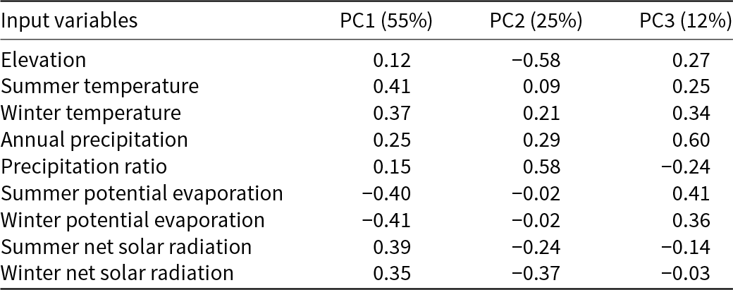
To define these glacier groups, we applied a Gaussian mixture model (GMM; Reynolds, Reference Reynolds2015) to the first three PCs. These first three PCs explain 92% of the total variance (Table 3). The GMM clustering was implemented using the Mclust package in R, specifying the VVV covariance structure (Scrucca and others, Reference Scrucca, Fop, Murphy and Raftery2016). In this formulation, each cluster is represented by its own ellipsoidal distribution, with volume, shape, and orientation all allowed to vary among clusters. This flexibility is useful because glacier groups in the PCA space are not expected to be spherical or equally dispersed, and may differ in overall spread, elongation and directional alignment. Model parameters were estimated using the Expectation–Maximization algorithm, which iteratively maximizes the overall log-likelihood until convergence (Dempster and others, Reference Dempster, Laird and Rubin1977). Each glacier was assigned to the cluster with the highest posterior probability.
PCA results showing eigenvectors of the input climate and topographic variables.

Table 3 Long description
The table lists principal component loadings for nine climate and topographic input variables across three components, with variance explained of 55% for PC1, 25% for PC2, and 12% for PC3. PC1 has the largest positive loadings for summer temperature (0.41), summer net solar radiation (0.39), winter temperature (0.37), and winter net solar radiation (0.35), while both summer and winter potential evaporation load strongly negative (−0.40 and −0.41). PC2 is dominated by precipitation ratio (0.58) and elevation loads strongly negative (−0.58), with winter net solar radiation also negative (−0.37). PC3 is most strongly associated with annual precipitation (0.60), with additional positive contributions from summer potential evaporation (0.41) and winter potential evaporation (0.36). Across components, precipitation ratio shifts from modestly positive on PC1 to strongly positive on PC2 and negative on PC3, indicating it separates a different gradient than total precipitation. Loadings indicate relative direction and strength within each component and should be interpreted as patterns rather than direct causal effects.
Note: Percentages in parentheses indicate the variance explained by each component (PC1 = 55%, PC2 = 25%, PC3 = 12%). PC1 is dominated by thermal variables (temperature, evaporation and radiation), PC2 by precipitation ratio (reflecting continentality) and PC3 by total annual precipitation.
The resulting six glacier clusters represent distinct climatic classes, within which glaciers are expected to respond similarly to climate forcing—reflected in similar CMI–MB slopes. To test this assumption, we conducted a leave-one-out cross-validation (LOOCV) within each cluster (Stone, Reference Stone1974). In each iteration, one glacier was excluded as a test case, and a linear regression between standardized CMI and MB was trained using the remaining glaciers in the same cluster. The trained model was then used to predict MB for the excluded glacier. Once all glaciers had been tested, we computed the root-mean-square error (RMSE) for each cluster to assess model performance.
Based on the validation, a cluster-specific linear regression model was constructed for each GMM cluster to represent its overall CMI–MB relationship. To test the advantages of regional modeling, these cluster-specific models were compared against a single global model trained across all glaciers. For demonstration, we applied this approach to the European Alps and identified 616 glaciers in the Alps from the RGI that were larger than 0.25 km2 and intersected by at least one MODIS pixel, representing 80.97% of the regional glacierized area. Each glacier was assigned to one of the previously defined climate clusters, and the corresponding cluster-specific CMI–MB regression was used for prediction. Annual standardized CMI values were calculated for each glacier from 2002 to 2021, yielding 12 320 glacier-years of estimates. Uncertainty was quantified by combining parameter covariance with residual variance to derive standard errors and prediction intervals. A regional estimate was then derived as the area-weighted average across all 616 glaciers.
4. Results
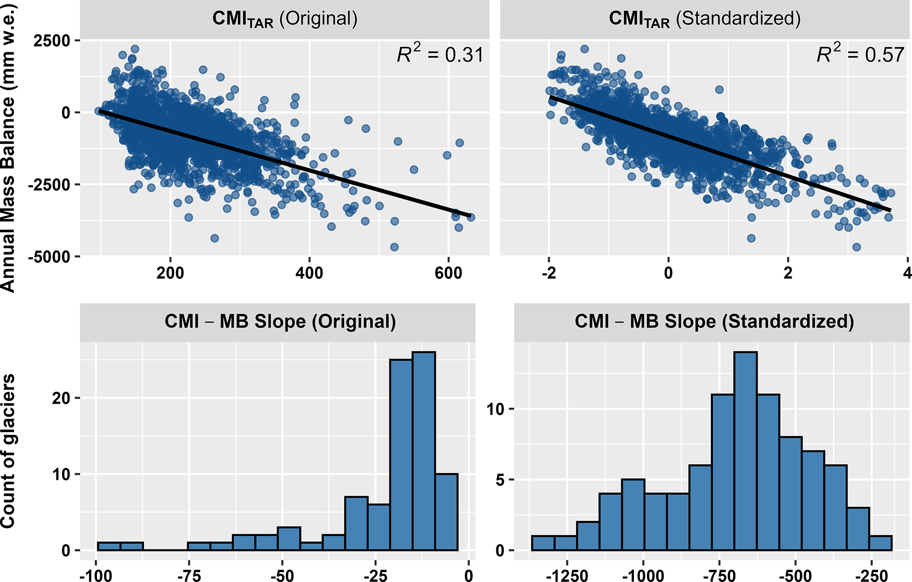
As an illustration of CMI standardization, Fig. 2 compares regressions based on raw and standardized CMI. Standardization compresses the spread of slopes across glaciers by removing differences associated with the scale of interannual CMI variability, making between-glacier comparisons easier to interpret. After standardization, the distribution of per-glacier CMI–MB slopes more closely approximates a normal distribution (Fig. 2 bottom panel). Additionally, the global-scale scatterplot (Fig. 2 top panel) of standardized CMI versus MB reveals a stronger linear relationship compared to regressions using raw CMI values. We therefore use standardized CMI in all subsequent analyses.
Overall CMI–MB relationship before and after standardization for the 88 glaciers in this study. Top panel: scatterplots using original (left) and standardized (right) CMI values. Bottom panel: distributions of corresponding CMI–MB regression slopes across all glaciers. CMI standardization reduces interglacier variability and produces a more consistent, approximately normal distribution.

Figure 2 Long description
First, a scatter plot titled CMI subscript TAR left parenthesis Original right parenthesis. Text on the plot reads R superscript 2 equals 0.31. The x-axis label reads CMI, with values 0 to 600. The y-axis label reads Annual Mass Balance left parenthesis millimeter w dot e dot right parenthesis, with values negative 500 to 250. Many circular markers form a cloud. A single fitted line slopes downward from left to right. Second, a scatter plot titled CMI subscript TAR left parenthesis Standardized right parenthesis. Text on the plot reads R superscript 2 equals 0.57. The x-axis label reads CMI, with values negative 2 to 4. The y-axis label reads Annual Mass Balance left parenthesis millimeter w dot e dot right parenthesis, with values negative 500 to 250. Many circular markers form a cloud. A single fitted line slopes downward from left to right. Third, a histogram titled CMI minus MB Slope left parenthesis Original right parenthesis. The x-axis label reads CMI minus MB Slope, with labeled ticks at negative 100, negative 75, negative 50, negative 25 and 0. The y-axis label reads Count of glaciers, with labeled ticks at 0, 10, 20 and 30. Bars are tallest near the tick labeled negative 25. Fourth, a histogram titled CMI minus MB Slope left parenthesis Standardized right parenthesis. The x-axis label reads CMI minus MB Slope, with labeled ticks at negative 1250, negative 1000, negative 750, negative 500 and negative 250. The y-axis label reads Count of glaciers, with labeled ticks at 0, 5, 10 and 15. Bars are tallest near the tick labeled negative 750. Across the two scatter plots, both fitted lines slope downward and the R superscript 2 values shown are 0.31 for Original and 0.57 for Standardized. Across the two histograms, the tallest bars occur near negative 25 for Original and near negative 750 for Standardized.
As summarized in Table 3, the first three PCs explain over 92% of the total variance in the selected climate variables. PC1 (55%) primarily reflects energy-related metrics—air temperature, potential evaporation and net solar radiation—thus distinguishing thermally warm from cold glacier environments. PC2 (25%) captures precipitation seasonality and continentality, separating low-elevation maritime glaciers from high-elevation continental glaciers, particularly those in central HMA. PC3 (12%) is dominated by annual precipitation and potential evaporation, highlighting contrasts in moisture availability and climatic aridity. Together, these components transform the climatic characteristics of glaciers into orthogonal dimensions representing energy input, precipitation seasonality and wetness, enabling clustering of similar glaciers regardless of geographic location.
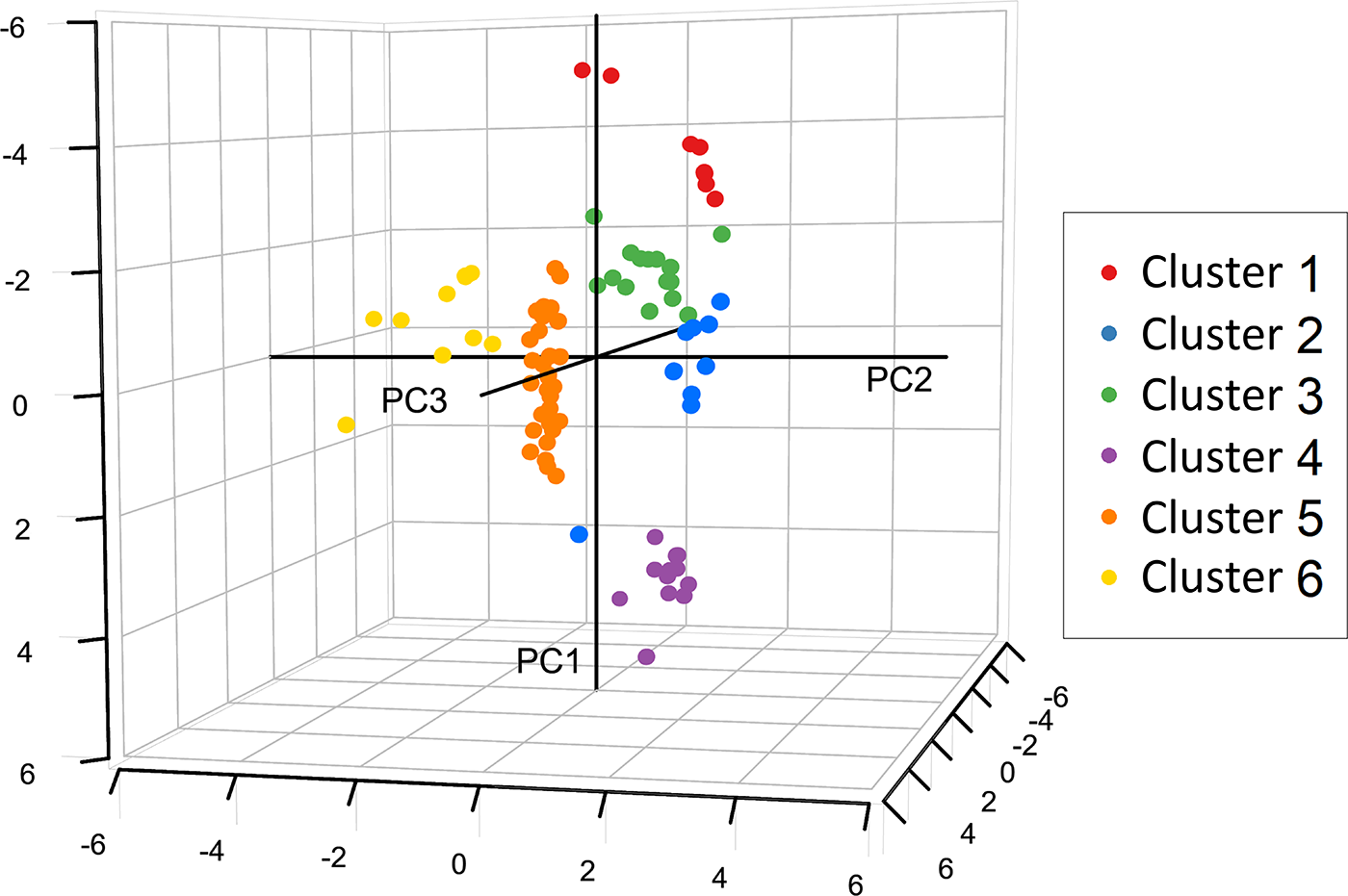
The projection of 88 glaciers into the PC space (PC1–PC3, as shown in Fig. 3) reveals six well-separated clusters as identified by the GMM. Each cluster occupies a distinct region in the PC space. For example, Cluster 1 glaciers exhibit the most negative PC1 values, indicating cold, low-radiation conditions, while Cluster 6 glaciers are characterized by the lowest PC2 values, signifying strong continentality.
Projection of studied glaciers in principal component space, color-coded by GMM cluster. Six clusters are well separated along the first three principal components.

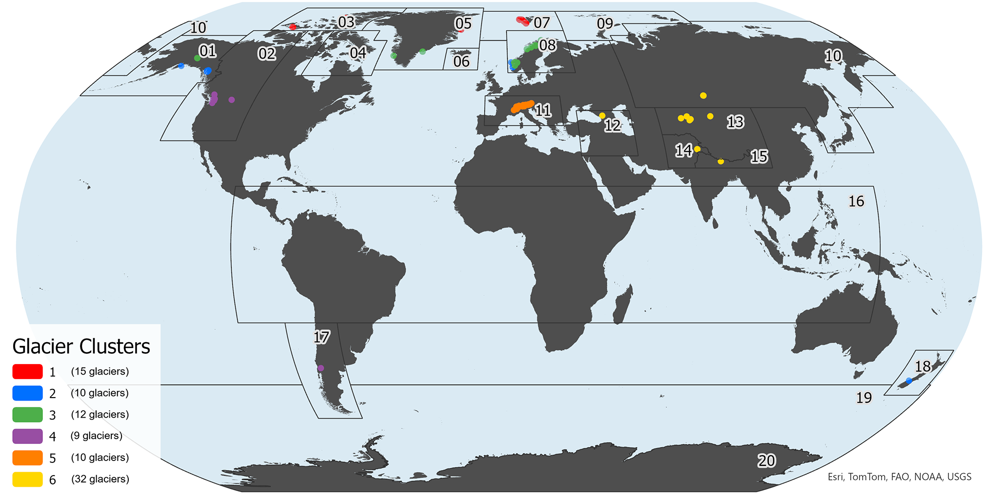
Figure 4 maps the geographic distribution of these clusters, showing that while some clusters are confined largely to a single RGI region, others span multiple regions. This supports the notion that GMM clustering is driven by climatic similarity rather than geographic proximity. Therefore, glaciers from different areas of the world that share similar climate characteristics are grouped together. These six clusters can be interpreted as follows:
1) Cluster 1 (15 studied glaciers) includes high-latitude polar glaciers (RGI Regions 3, 5 and 7). These glaciers experience the coldest temperatures, lowest incoming solar radiation and exhibit the flattest standardized CMI–MB slopes.
2) Cluster 2 (10 glaciers) represents high-latitude maritime glaciers found in Alaska, southern Norway and New Zealand. These glaciers are characterized by persistent year-round precipitation and high MB variability.
3) Cluster 3 (12 glaciers) mainly comprises Norwegian glaciers (RGI Region 8) with colder conditions and less precipitation compared to Cluster 2.
4) Cluster 4 (9 glaciers) consists primarily of maritime glaciers in the northwestern United States, with one glacier in the Southern Andes. These glaciers have the highest precipitation ratios and strong maritime influence, resulting in high CMI sensitivity.
5) Cluster 5 (10 glaciers) includes mid-latitude alpine glaciers in the European Alps (RGI Region 11). These glaciers typically have high median elevations and more balanced seasonal precipitation, distinguishing them from Cluster 4.
6) Cluster 6 (32 glaciers) contains mostly continental glaciers, located in HMA (RGI Regions 12–14). These glaciers reside at high elevations and have the lowest precipitation ratios among all clusters.
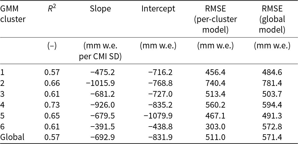
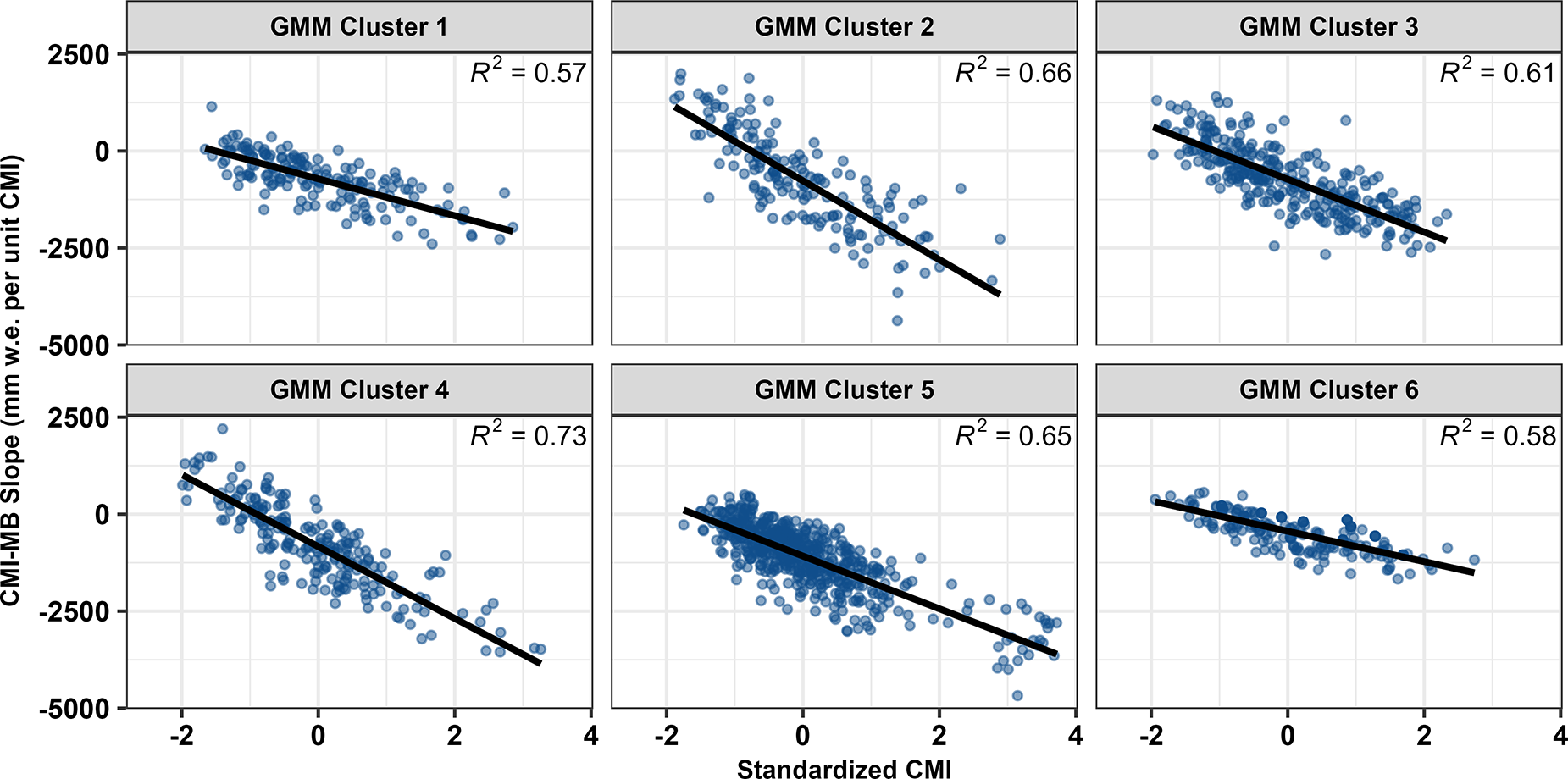
Compared to the single global regression using all glacier-year observations together (Fig. 2), the cluster-specific regressions (Fig. 5; Table 4) show more coherent CMI–MB relationships and lower cross-validated RMSE. This supports the established glaciological understanding that region-specific regression models are more suitable than a single global model. Accordingly, we fitted six separate linear regressions—one for each GMM-derived cluster—relating standardized CMI to annual MB. The resulting slopes, intercepts and coefficients of determination (R 2) are summarized in Table 4, with most clusters showing strong relationships (R 2 > 0.6). Among these six clusters, Clusters 2 and 4 exhibit the steepest slopes, whereas Clusters 1 and 6 show flatter slopes.
Spatial distribution of the six GMM clusters for the 88 studied glaciers worldwide. Glaciers within the same cluster often occur in close geographic proximity, reflecting shared climatic conditions.

Figure 4 Long description
The map is a thematic representation of glacier clusters worldwide, oriented with north at the top. It categorizes glaciers into six clusters, each represented by a different color. The legend specifies: Red for 15 glaciers, Blue for 10 glaciers, Purple for 12 glaciers, Green for 9 glaciers, Orange for 10 glaciers and Yellow for 32 glaciers. Each cluster is marked with a numbered label on the map. The red cluster is located in high-latitude polar regions. The blue cluster appears in high-latitude maritime areas. The purple cluster is mainly in Norwegian regions. The green cluster is found in maritime areas of the northwestern United States and the Southern Andes. The orange cluster is in mid-latitude alpine regions of the European Alps. The yellow cluster is primarily in continental regions of High Mountain Asia. The map includes numbered labels for each cluster, enhancing identification and understanding of their geographic distribution.
Linear regression results between standardized CMI and annual glacier mass balance for each GMM cluster.

Table 4 Long description
The table reports linear regression performance linking standardized CMI to annual glacier mass balance for six GMM clusters and a global model, using R2, slope, intercept, and cross-validated RMSE. All clusters show negative slopes, meaning higher CMI is associated with more negative mass balance. The best fit is Cluster 4 with R2 0.73 and slope minus 926.0 mm water equivalent per CMI standard deviation; Cluster 2 is next with R2 0.66 and the steepest slope at minus 1015.9. The weakest fits are Cluster 1 and the global model, both with R2 0.57. Per-cluster RMSE ranges from 303.0 in Cluster 6 to 740.4 in Cluster 2, while the global-model RMSE column ranges from 484.6 to 781.4 across clusters. In most clusters the per-cluster RMSE is lower than the global-model RMSE, with the largest improvement in Cluster 6 (303.0 versus 572.8), but Cluster 3 is a small exception where the per-cluster RMSE is slightly higher than the global-model RMSE (513.4 versus 503.7). Intercepts are all negative, spanning from minus 438.8 in Cluster 6 to minus 1079.9 in Cluster 5. RMSE values come from leave-one-out cross-validation, so they reflect predictive error rather than in-sample fit.
Note: RMSE values are from leave-one-out cross-validation. In most clusters, the per-cluster models outperform the global model.
Scatterplots of standardized CMI versus annual glacier mass balance for the 88 studied glaciers, grouped by Gaussian mixture model (GMM) cluster. Within each cluster, glaciers show broadly consistent slopes and intercepts, with maritime clusters (e.g. 2 and 4) exhibiting steeper negative slopes than polar or continental clusters (e.g. 1 and 6).

Figure 5 Long description
The image showing six scatter plots titled “GMM Cluster 1”, “GMM Cluster 2”, “GMM Cluster 3”, “GMM Cluster 4”, “GMM Cluster 5” and “GMM Cluster 6”. Each plot contains point markers and a single straight fitted line. For all six plots, the horizontal axis label is “Standardized CMI”. The horizontal axis tick labels shown are negative 2, 0, 2 and 4. For all six plots, the vertical axis label is “CMI MB slope (mm w.e. per unit CMI)”. The vertical axis tick labels shown are 2500, 0, negative 2500 and negative 5000. GMM Cluster 1: Text “R superscript 2 equals 0.57”. The fitted line slopes downward from left to right. GMM Cluster 2: Text “R superscript 2 equals 0.66”. The fitted line slopes downward from left to right. GMM Cluster 3: Text “R superscript 2 equals 0.61”. The fitted line slopes downward from left to right. GMM Cluster 4: Text “R superscript 2 equals 0.73”. The fitted line slopes downward from left to right. GMM Cluster 5: Text “R superscript 2 equals 0.65”. The fitted line slopes downward from left to right. GMM Cluster 6: Text “R superscript 2 equals 0.58”. The fitted line slopes downward from left to right.
By using LOOCV, we assessed the predictive performance of region-specific models. In each iteration, one glacier was excluded for testing, while the remaining glaciers in the cluster were used to train a linear regression model. The excluded glacier’s MB was then predicted, and the process was repeated for all glaciers. The resulting RMSE values for each cluster are presented in Table 4. The highest RMSE of 740.4 mm w.e. for Cluster 2 likely reflects greater interannual variability in MB due to its maritime climate setting. As a benchmark, we also applied a single global linear regression model between standardized CMI and annual MB across all 88 studied glaciers. The global model performs reasonably well, yielding an R 2 of 0.57, an RMSE of 571.4 mm w.e. and a slope of −692.9 mm w.e. per SD of CMI. When predictions from the cluster-specific models are pooled across all glaciers, the overall RMSE decreases to 511.0 mm w.e., indicating better predictive performance than the global model. We also calculated RMSE values for each GMM cluster using the global model, summarized in the final column of Table 4. In five out of the six clusters, the per-cluster models produced notably lower RMSE values than the global model, underscoring the value of region-specific modeling. For Cluster 3, however, the per-cluster RMSE was slightly higher than the global model RMSE. Notably, the slope and intercept for Cluster 3 closely match those of the global model, suggesting that Cluster 3 glaciers may represent the average behavior of alpine glaciers globally.
Table 5 provides a descriptive summary of the main characteristics of each GMM cluster. The clusters differ not only in their mean PCA scores, which reflect different climatic settings, but also in glacier elevation and MB behavior. For example, Cluster 6 has the highest mean glacier elevation (4041 m a.s.l.) and the lowest variability in annual MB (SD = 208.5 mm w.e. yr−1), whereas Cluster 2 shows the largest MB variability (SD = 603.9 mm w.e. yr−1). Cluster 5 has the most negative mean annual MB (−1083.3 mm w.e. yr−1), while Clusters 1 and 4 are also characterized by strongly negative mean MB (about −799 mm w.e. yr−1). These summaries help quantify the differences among clusters and provide context for interpreting why the standardized CMI–MB relationships differ among climate groups.
Descriptive summary of glacier and climate characteristics for each GMM cluster, including cluster-mean annual mass balance, standard deviation of annual mass balance, mean PCA scores and mean glacier elevation above sea level.

Table 5 Long description
The table summarizes six Gaussian mixture model clusters using mean annual glacier mass balance and its year-to-year variability, three mean principal component scores, and mean glacier elevation. Mean annual mass balance is negative for all clusters, ranging from −509.99 mm w.e. in cluster 6 to −1083.28 mm w.e. in cluster 5. Cluster 6 pairs the highest mean elevation, 4041.1 m, with the least negative mean mass balance and a low standard deviation of 208.5 mm w.e. Cluster 5 has the most negative mean mass balance and a mid-range standard deviation of 357.88 mm w.e., with mean elevation 2979.5 m. The largest variability occurs in cluster 2, with a standard deviation of 603.94 mm w.e., while cluster 4 shows the smallest variability at 226.2 mm w.e. Principal component patterns differ by cluster: cluster 4 has the highest mean PC1 score at 4.18, and cluster 6 has the lowest mean PC2 score at −2.84. Values are cluster means, so they describe typical conditions within each group and do not show within-cluster distributions or causal relationships.
A further limitation arises from mixed MODIS pixels, particularly for small glaciers and glaciers with narrow tongues. In our earlier TAR/CMI analysis, we used an 80% glacier-coverage threshold to ensure that selected pixels primarily represent glacier surfaces; however, even with this threshold, some glaciers may be represented mainly by broader upper zones rather than narrow ablation tongues. This can bias the derived phenology metrics, and in summer the inclusion of off-glacier bedrock within partially filled pixels may elevate LST above glacier-surface conditions, thereby distorting TAR and CMI. These effects are expected to be strongest for small, debris-covered or geometrically narrow glaciers, and they motivate our current application limit of 0.25 km2.
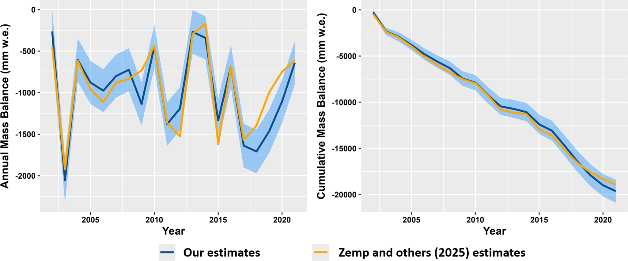
For the European Alps application, we identified 616 glaciers larger than 0.25 km2, and their distribution is shown in Supplementary Fig. S1. Of the 616 glaciers, the majority (i.e. 534) were classified as Cluster 5 (typical European Alps glaciers), 80 as Cluster 6 (colder, more continental), and 2 as Cluster 2 (warmer, maritime). The corresponding cluster-specific CMI–MB models were applied to estimate annual MB for each glacier. Over the study period, the area-weighted mean annual MB was −981.9 ± 11 mm w.e. a−1. This estimate is broadly consistent with the community-based regional observational estimate from the Glacier Mass Balance Intercomparison Exercise (GlaMBIE) reported by Zemp and others (Reference Zemp2025), who reported a mean annual MB of −1.06 ± 0.04 m w.e. a−1 for the European Alps over 2000–23, equivalent to −1060 ± 40 mm w.e. a−1. Because the two estimates are derived from different methods and cover slightly different periods, they are not directly identical, but their close agreement supports the realism of the CMI-based regional application. Figure 6 shows the area-weighted mean annual MB of these 616 glaciers, with a cumulative mass loss of 19 638.2 ± 222 mm w.e.
Annual glacier mass balance from 2002 to 2021 for 616 glaciers in the European Alps. Left: annual mass balance. Right: cumulative mass balance. The blue curve shows regional CMI-based estimates derived from cluster-specific regression models, with shaded areas indicating 95% prediction intervals, while the yellow curve shows annual estimates from Zemp and others (Reference Zemp2025). The regional model shows good agreement with the independent GlaMBIE-based regional estimate from Zemp and others.

5. Discussion
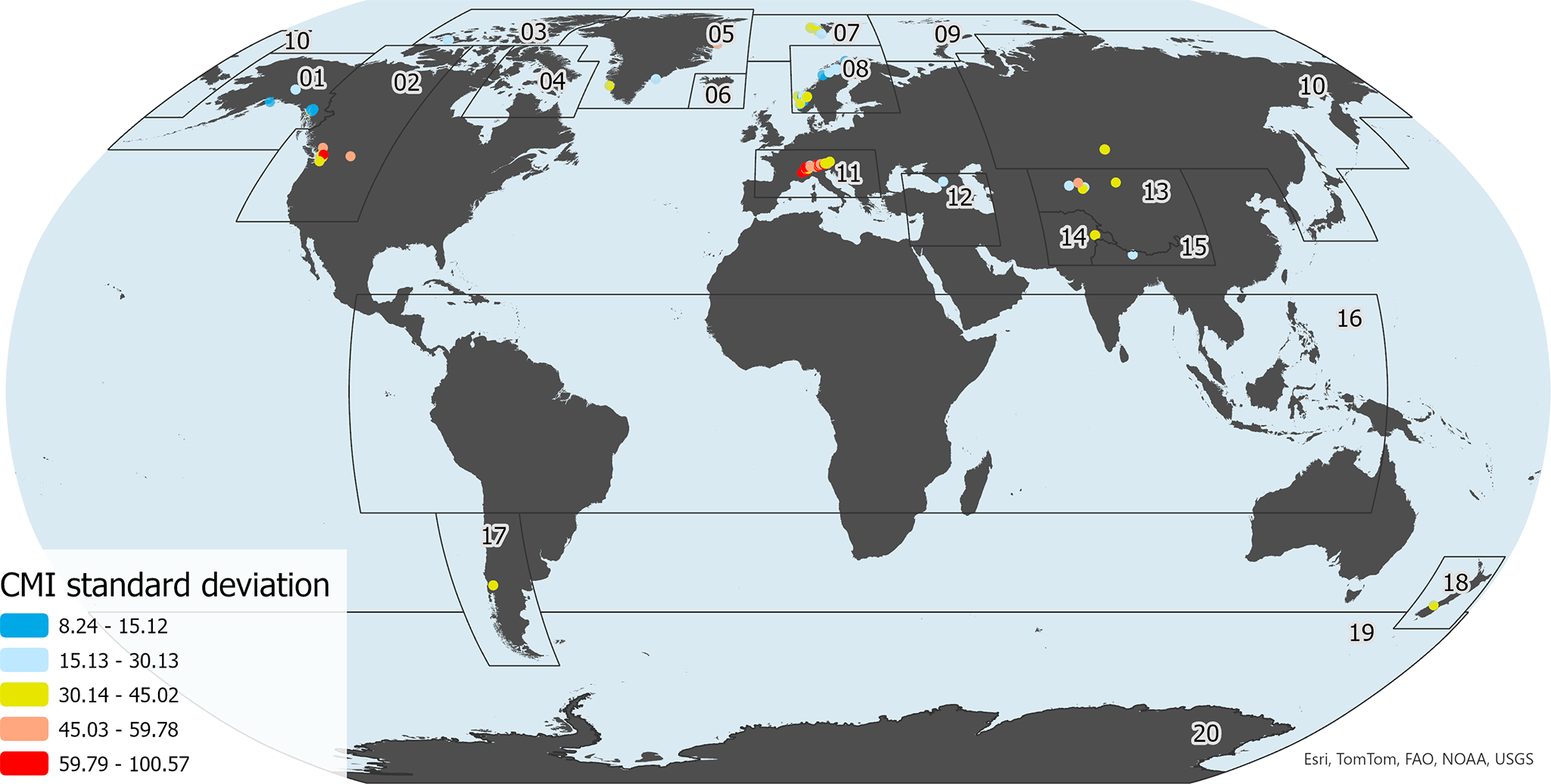
The spatial distribution of interannual CMI SD (Fig. 7) helps explain why raw CMI–MB slopes are difficult to compare directly among glaciers. Glaciers differ substantially in the year-to-year variability of CMI, with persistently cold polar glaciers generally showing lower CMI variability than more temperate maritime glaciers. As a result, raw regression slopes reflect not only differences in MB response but also differences in the scale of CMI variability itself. Standardizing CMI removes this glacier-specific scaling effect and allows the slope to be interpreted as the change in annual MB associated with a 1 SD anomaly in CMI. In this form, the slope is more suitable for interglacier comparison, while the remaining differences among clusters can be interpreted in relation to broader climatic settings. Previous studies using albedo-based glacier metrics have also shown that remotely sensed surface indicators can correlate strongly with annual MB, while their sensitivity varies substantially among glaciers and regions (Dumont and others, Reference Dumont2012; Davaze and others, Reference Davaze2018; Di Mauro and Fugazza, Reference Di Mauro and Fugazza2022). Our standardization step provides a more consistent basis for comparing those sensitivities across contrasting glacier environments.
Standard deviation of CMI for the 88 studied glaciers worldwide, representing interannual variability in glacier-surface conditions. Warm, maritime glaciers generally show higher variability than cold, continental glaciers.

Figure 7 Long description
A thematic world map with north at the top shows “CMI standard deviation” at numbered point locations. A legend titled “CMI standard deviation” lists five classes: 8.24 - 15.12; 15.13 - 30.13; 30.14 - 45.02; 45.03 - 59.78; 59.79 - 100.37. The mapped points are concentrated in high-latitude and mountain regions, including clusters in northwestern North America, the North Atlantic region near Greenland and Iceland, mainland Europe, central and southern Asia, the southern Andes and New Zealand. The highest class (59.79 - 100.37) appears at a small number of sites, including several in mainland Europe and at least one in northwestern North America. The lowest class (8.24 - 15.12) appears at multiple sites, including several in the North Atlantic region near Greenland and Iceland and across parts of northern Eurasia. Each point is paired with a small number label that functions as a site identifier. Visible identifiers include 01, 02, 03, 04, 05, 06, 07, 08, 09, 10, 11, 12, 13, 14, 15, 16, 17, 18, 19 and 20.
As shown in Fig. 5, the contrast in cluster-specific CMI–MB slopes is broadly consistent with established glaciological understanding of regional differences in glacier climate sensitivity. Maritime glaciers, represented here by Clusters 2 and 4, typically experience mild, humid conditions and strong ablation-season energy exchange, so interannual variations in melt-season surface conditions can be translated more directly into annual MB anomalies. This interpretation is consistent not only with traditional temperature-index and MB studies (Braithwaite, Reference Braithwaite1995; Oerlemans and Reichert, Reference Oerlemans and Reichert2000; Hock, Reference Hock2005) but also with broader literature showing that regional glacier MB variability reflects interacting controls of temperature, precipitation seasonality and large-scale atmospheric forcing (Lewis and Smith, Reference Lewis and Smith2004; Christian and others, Reference Christian, Siler, Koutnik and Roe2016; Bonan and others, Reference Bonan, Christian and Christianson2019; Zhu and others, Reference Zhu, Thompson, Zhao, Yao, Yang and Jin2021). By contrast, the flatter slopes found for Clusters 1 and 6 suggest that interannual variability in CMI is associated with a weaker MB response in polar and continental settings, where melt is more strongly constrained by low temperatures, limited moisture availability or both. For HMA glaciers in Cluster 6, this weaker sensitivity may also partly reflect glacier-specific factors such as debris cover, which can decouple surface thermal conditions from total ablation.
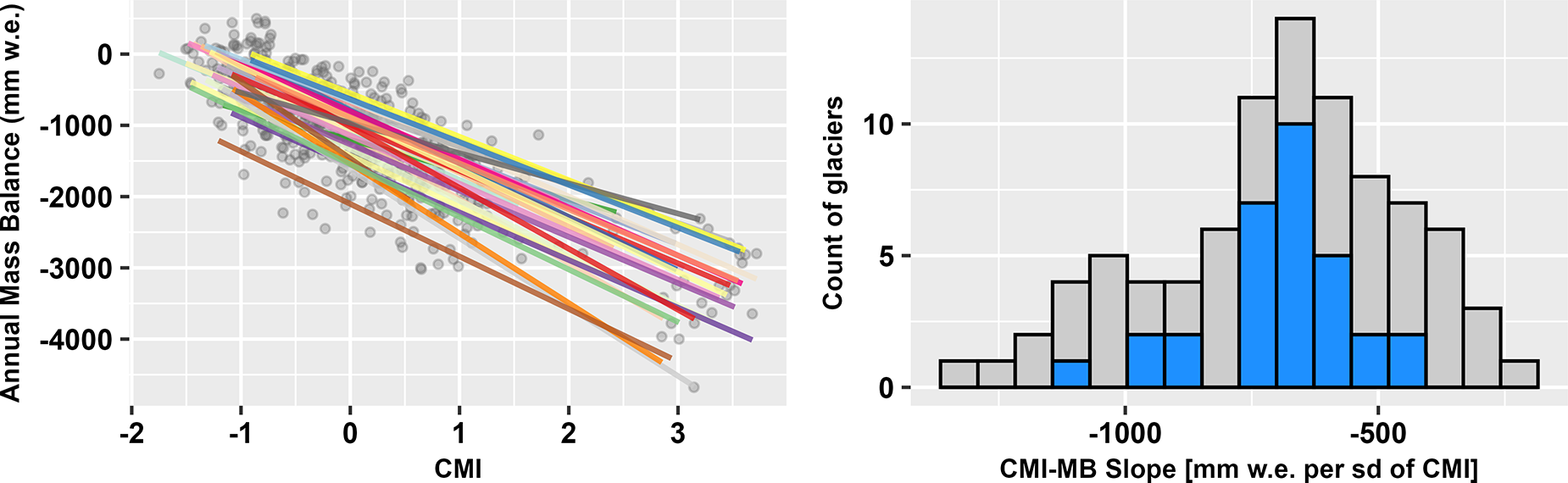
To further examine variability in CMI–MB slopes within each cluster, we performed individual linear regressions for each glacier. The results for Cluster 5 are shown in Fig. 8. The left panel displays the per-glacier fitted lines, while the right panel shows the distribution of slopes from these regressions. Most glaciers exhibit slopes consistent with the overall Cluster 5 regression (−692.1 ± 51.3 mm w.e. per SD of CMI; Cluster 5 model slope = −679.5 mm w.e. per SD of CMI), whereas intercepts display greater variability (−1076.5 ± 126.8 mm w.e.; Cluster 5 model intercept = −1079.9 mm w.e.). No significant correlations were found between the intercepts and the ERA5 climate variables included in this study, suggesting that this variability is not well explained by the broad climatic descriptors used here. Instead, it may reflect glacier-specific characteristics not resolved in the present analysis, such as elevation, aspect, hypsometry, shading, debris cover or local snow-accumulation processes. Intercept variability therefore appears to be a plausible source of residual error in the LOOCV. Equivalent plots for the remaining five clusters are provided in the Supplementary material.
Per-glacier CMI–MB linear regressions and corresponding slope distribution for Cluster 5 glaciers. Left: relationship between standardized CMI and annual MB, with per-glacier linear fits color-coded for each glacier. Right: distribution of CMI–MB slopes, with gray bars showing all 88 studied glaciers and blue bars highlighting glaciers in Cluster 5. Glaciers in this cluster exhibit broadly consistent slopes, while intercepts display greater variability.

Figure 8 Long description
The image A showing a scatter plot with multiple straight fitted lines overlaid on the points. The horizontal axis label is CMI, with tick labels negative 2, negative 1, 0, 1, 2, 3. The vertical axis label is Annual mass balance (mm w.e.), with tick labels 0, negative 1000, negative 2000, negative 3000, negative 4000. The fitted lines slope downward from left to right. The plotted points form a band spanning from near 0 down to near negative 4000 across the horizontal axis range. The image B showing a histogram. The horizontal axis label is CMI-MB Slope (mm w.e. per sd of CMI), with tick labels negative 1000, negative 500, 0. The vertical axis label is Count of glaciers, with tick labels 0, 5, 10, 15. Bars span the horizontal axis range from about negative 1200 to about 0. The tallest bar is near the middle of the distribution, slightly left of negative 500, reaching a height a little above 15. Several bars in the central range are highlighted and the remaining bars extend on both sides with lower heights.
Although Fig. 6 shows that the CMI-based regional estimate reproduces the overall temporal pattern of the GlaMBIE series for the European Alps, larger discrepancies are evident during 2018–20. These differences likely reflect the climatic anomalies of those years. CMI primarily captures ablation-season surface conditions, including low albedo, high surface temperature and prolonged exposure of bare ice, but it does not explicitly represent winter accumulation. In the Swiss Alps, 2017/18 and 2018/19 were characterized by above-average winter snow amounts followed by exceptionally strong summer melt, so a melt-season metric such as CMI may record a stronger anomaly than the final annual MB (GLAMOS, 2020). The discrepancy during these years therefore likely reflects the contrast between a melt-season remote-sensing proxy and a regional annual MB benchmark that integrates both accumulation and ablation processes more completely.
We should point out that the proposed CMI–MB estimation procedure is currently limited to glaciers larger than 0.25 km2, due to the spatial resolution constraints of MODIS. Future work should aim to overcome this limitation by integrating higher-resolution satellite products. One promising direction is the use of the Harmonized Landsat–Sentinel dataset, which combines the spatial resolution of Landsat with the temporal frequency of Sentinel-2 (Claverie and others, Reference Claverie2018). This would allow more accurate monitoring of smaller or debris-covered glaciers and improve the precision of phenology-based melt metrics such as CMI. In addition, expanding this framework to include currently excluded glacier types—such as tropical and monsoon-influenced glaciers—will require adapting the method to regions where CMI and MB show weaker correlations. Incorporating other satellite observations, such as radar or LiDAR to measure changes in ice thickness may enhance the ability to directly link glacier-surface changes to volume loss (Abdalati and others, Reference Abdalati2010; O’Loughlin and others, Reference O’Loughlin, Neal, Yamazaki and Bates2016; Paul and others, Reference Paul2017), providing a more comprehensive understanding of glacier mass change across diverse climatic regimes.
6. Conclusion
This study investigates the variability of the relationship between CMI and annual glacier MB across 88 alpine glaciers worldwide. By standardizing CMI values for each glacier and analyzing the resulting slopes, we stabilized the relationship and improved comparison of MB responses to phenology metrics across glaciers. The remaining interglacier variability in CMI–MB slopes likely reflects differences in regional climate and glacier characteristics. To account for regional climate variability, we applied PCA and GMM to classify glaciers into six climatically coherent clusters based on their climatic properties, each exhibiting distinct energy and moisture regimes.
The results demonstrate that standardized CMI–MB slopes vary systematically with climate, with maritime glaciers showing the steepest slopes and polar or continental glaciers exhibiting weaker responses. The use of cluster-specific regression models significantly improved estimation accuracy, with a pooled RMSE of 511.0 mm w.e., compared with 571.4 mm w.e. for a single regression model. The regional application of this approach based on 616 glaciers in the European Alps yielded a 20 year annual average mass loss estimate of −981.9 ± 11 mm w.e. a−1, broadly consistent with the GlaMBIE community-based regional observational estimate.
These findings highlight the value of MODIS-based phenology metrics, such as CMI, for large-scale glacier MB estimation. Using remote-sensing observations alone, MB can be inferred for glaciers lacking direct in situ measurements through the region-specific regression models developed in this study. The cluster-specific approach enables flexible regional modeling, even across widely separated geographic regions, by grouping glaciers with similar climate responses rather than relying on location alone. This framework can support long-term monitoring of glacier change under global warming and contribute to improved hydrological forecasting in glacier-fed basins.
Supplementary material
The supplementary material for this article can be found at https://doi.org/10.1017/jog.2026.10174.
Data availability statement
MODIS albedo data can be accessed through Google Earth Engine: https://developers.google.com/earth-engine/datasets/catalog/MODIS_061_MOD10A1. Glacier mass-balance data can be downloaded from WGMS website: https://wgms.ch/mass_change_estimates/.
Competing interests
No potential conflicts of interest were reported by the authors.



 Open access

