2. CONTROL PROBLEM AND NONLINEAR FEEDBACK TECHNIQUE

Consider a course keeping problem for ships, the controlled plant G is taken as the nominal Nomoto model when the controller K is designed using the first order closed loop gain shaping algorithm without considering the nonlinear feedback (Zhang and Wang, Reference Zhang and Wang2010; Aarsaether and Moan, Reference Aarsaether and Moan2010). A robust controller for a standard feedback system is solved below under the following three predetermined conditions: the bandwidth frequency of the closed system being 1/T ₁ (1/T ₁ should be the crossover frequency in the strict sense, and is approximately regarded as bandwidth frequency for the sake of easy analysis), the largest singular value being unity, and the high frequency asymptote slope being −20 dB/dec. The frequency spectrum of the closed-loop system is made equal to the frequency spectrum of a first-order inertial system with the largest singular value approximately one (Zhang and Wang, Reference Zhang and Wang2010), i.e.

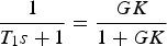$$\displaystyle{1 \over {{T_1}s + 1}} = \displaystyle{{GK} \over {1 + GK}}$$

The course keeping controller is then solved as

(1)$$K(s) = \displaystyle{1 \over {G{T_1}s}}$$

The ship model being a standard Nomoto model is expressed in Equation (2) where ψ is the heading angle, δ is the rudder angle, K ₀ and T ₀ are the manoeuvrability indices of the ship.

(2)$$G(s) = \displaystyle{\psi \over \delta} = \displaystyle{{{K_0}} \over {s\left( {{T_0}s + 1} \right)}}$$

To eliminate the steady state error using the closed loop gain shaping algorithm, a minor constant ε (0·01) is added into the denominator of the Nomoto model. Then, Equation (3) is obtained

(3)$$G(s) = \displaystyle{{{K_0}} \over {{T_0}{s^2} + s + \varepsilon}} $$

Actually, ε can derive the integral effect for the designed controller and it also reproduces the effect of uncertain constant disturbance upon the closed-loop system. When ε is too small, the control law may be with the static error or the long setting time. When ε is too large, the system output tracks the reference signal with the overshooting dynamics. Therefore one should trade off the two terms by selecting the parameter ε properly.

Thus, substitute Equation (3) into Equation (1), according to closed loop gain shaping algorithm, a linear Proportional-Integral-Differential (PID) controller is obtained

(4)$$K(s) = \displaystyle{1 \over {{K_0}{T_1}}} + \displaystyle{\varepsilon \over {{K_0}{T_1}}}\displaystyle{1 \over s} + \displaystyle{{{T_0}} \over {{K_0}{T_1}}}s$$

In actual application, we discover that the settling time is relatively long for ships with large time constants such as oil tankers etc. The dynamic performance of course keeping control systems for ships can be improved greatly when a positive constant ρ is added to the proportional part of the control law, Equation (4). Finally, the actual controller is presented in Equation (5). The corresponding theoretical analysis and simulation test are given in reference Zhang (Reference Zhang and Zhang2012).

(5)$$K(s) = \displaystyle{1 \over {{K_0}{T_1}}} + \rho + \displaystyle{\varepsilon \over {{K_0}{T_1}}}\displaystyle{1 \over s} + \displaystyle{{{T_0}} \over {{K_0}{T_1}}}s$$

A nonlinear feedback system driven by a sine function is shown in Figure 1. Contrary to the standard feedback configuration, sin (ω ₁(r − y)) where ω ₁ is the design parameter substituted for (r − y). Note that the block diagram of sin (ω ₁(r − y)) shown in Figure 1 does not conform to its standard graphical representation. How to find a stable K with fine control performance in δ = K(r − y) is the main work in the previous research no matter whether K is linear or nonlinear, but in this section the main work is how to test the better control performance of the nonlinear feedback control in the form of δ = K sin (ω ₁(r − y)) under the same controller K.

Figure 1.

The block diagram of a nonlinear feedback system.

The effects of nonlinear feedback on the dynamic and static performance are analysed by using sin (ω ₁(r − y)) ≈ ω ₁(r − y) when the error is small. The demonstration process is presented in Zhang (Reference Zhang2011). In some situations, this assumption may not be tenable when the error is large. The effects of nonlinear feedback driven by sine function to the closed system can be analysed by Taylor series expansion:

(6)$$\displaylines{\sin \left( {{\omega _1}\left( {r - y} \right)} \right) \approx {\omega _1}\left( {r - y} \right) - {{{{\left( {{\omega _1}\left( {r - y} \right)} \right)}^3}} / {3!}} \cr + {{{{\left( {{\omega _1}\left( {r - y} \right)} \right)}^5}} / {5!}} - \cdots} $$

Let the error e = r − y, Equation (6) is simplified up to the third order, then

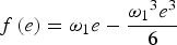(7)$$f\,(e) = {\omega _1}e - \displaystyle{{{\omega _1}^3 {e^3}} \over 6}$$

According to Hu (Reference Hu2007), if the error input e of Equation (7) is Asin ω ₀t, then the output of the nonlinear system in Equation (7) can be approximated by its first order harmonic element, and the equivalent frequency characteristics is the describing function of the nonlinear system.

Let the output of Equation (7) be f(t) under the sine input Asin ω ₀t, then its output can be expressed as Equation (8) using its first order harmonic element of the Fourier series (Ciaurri et al., Reference Ciaurri, Perez, Reyes and Varona2010).

(8)$$f(t) = {A_0} + {A_1}\cos {\omega _0}t + {B_1}\sin {\omega _0}t$$

where A ₀ is the DC component, A ₁, B ₁ are the first order harmonic components, and

$$\left\{ \matrix{{A_1} = \displaystyle{1 \over {\rm \pi}} \int_0^{2{\rm \pi}} {\,f\,{\rm (t)}} \cos {\omega _0}t{\rm d}{\omega _0}t,\quad \hfill \cr {B_1} = \displaystyle{1 \over {\rm \pi}} \int_0^{2{\rm \pi}} {\,f\,{\rm (t)}} \sin {\omega _0}t{\rm d}{\omega _0}t,\quad \hfill \cr {A_0} = \displaystyle{1 \over {{\rm 2\pi}}} \int_0^{2{\rm \pi}} {\,f\,{\rm (t)}} {\rm d}{\omega _0}t \hfill} \right.$$

Under the action of sine input signal e in Equation (7), the complex ratio of its first order harmonic element in the steady state output to its input signal is referred to the describing function which is expressed as N(A).

$$N(A) = \displaystyle{{{B_1} + {\rm j}{A_1}} \over A}$$

Equation (7) is an odd function, thus A ₀ = 0. When e = Asin ω ₀t

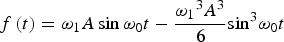(9)$$f\,(t) = {\omega _1}A\sin {\omega _0}t - \displaystyle{{{\omega _1}^3 {A^3}} \over 6}{\sin ^3}{\omega _0}t$$

Equation (9) is also an odd function of t, so A ₁ = 0. Because of the semi-cyclic symmetry property of f(t), then

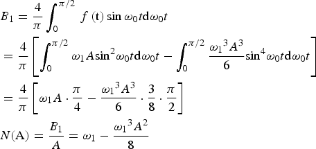(10)$$\eqalign{& {B_1} = \displaystyle{4 \over {\rm \pi}} \int_0^{{\rm \pi /2}} {\,f\,{\rm (t)}} \sin {\omega _0}t{\rm d}{\omega _0}t \cr & = \displaystyle{4 \over {\rm \pi}} \left[\int_0^{{\rm \pi /2}} {{\omega _1}A} {\sin ^2}{\omega _0}t{\rm d}{\omega _0}t - \int_0^{{\rm \pi /2}} {\displaystyle{{{\omega _1}^3 {A^3}} \over 6}} {\sin ^4}{\omega _0}t{\rm d}{\omega _0}t\right] \cr & = \displaystyle{4 \over {\rm \pi}} \left[{\omega _1}A \cdot \displaystyle{{\rm \pi} \over 4} - \displaystyle{{{\omega _1}^3 {A^3}} \over 6} \cdot \displaystyle{3 \over 8} \cdot \displaystyle{{\rm \pi} \over 2}\right] \cr & N{\rm (A)} = \displaystyle{{{B_1}} \over A} = {\omega _1} - \displaystyle{{{\omega _1}^{\rm 3} {A^2}} \over 8}} $$

In the light of the physical meaning of frequency characteristics, the system in Figure 1 is equivalent to the system shown in Figure 2. Effects of the nonlinear feedback driven by sine function can be analysed as follows.

Figure 2.

Equivalent block diagram of a nonlinear feedback system.

2.1. Effect on the steady state of the closed loop system

Let the reference input be a step signal, its amplitude is r, the steady state error to the step input is obtained directly by the final value theorem as given below:

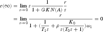$$\eqalign{e(\infty ) & = \mathop {\lim }\limits_{s \to 0} s\displaystyle{1 \over {1 + GKN(A)}}\displaystyle{r \over s} \cr & = \mathop {\lim }\limits_{s \to 0} \displaystyle{r \over {1 + (\displaystyle{1 \over {{T_1}s}} + \rho \displaystyle{{{K_0}} \over {s({T_0}s + 1)}}){\omega _1}}} = 0}$$

Therefore the nonlinear feedback driven by sine function has no extra effect to the steady state of the system.

2.2. Effect on the dynamic performance of the closed loop system

Based on the block diagram of the nonlinear feedback system shown in Figure 2, the transfer function from the input r (i.e. the setting course ψ _r) to the output y of the system (i.e. the heading angle ψ) can be obtained as Equation (11).

(11)$$\displaystyle{y \over r} = \displaystyle{{GKN(A)} \over {1 + GKN(A)}}$$

For the ship course keeping problem, wave action is a high frequency disturbance whose frequency spectrum lies in the range of 0·3~1·25 rad/s. Generally 1/T ₁ < 0·3 rad/s is taken in Equation (10) to shy away from the wave frequency spectrum. Suppose the range of course changing is between 0~2π rad, then 0 < N(A) ≤ ω ₁. The Loop Shaping algorithm of H _∞ robust control theory is a type of open-loop gain shaping method (Zhang, Reference Zhang2012). Its key point lies in finding a controller K to make the gains $\underline \sigma (GK)$ and $\bar \sigma (GK)$ of the open-loop transfer matrix GK satisfy robust performance in the low frequency zone and robust stability in the high frequency zone, i.e. high gain in the low frequency zone and low gain in the high frequency zone. The loop shaping algorithm implements the closed-loop performance of the system through selecting weighting functions to shape the open-loop frequency characteristic curve, and obtains an acceptable performance/robustness trade-off. According to the loop shaping theory, if Equation (11) is compared to the closed loop transfer function GK/(1 + GK) of a standard feedback system, the introduction of N(A) has less effect on the dynamic performance of the system because of the high gain of GK in the low frequency zone and 0 < N(A) ≤ 1. Thus the proper trade-off between the stabilising performance and robustness can be obtained by selecting the corresponding parameter setting appropriately.

2.3. Effect on the output of the closed loop system

The transfer function from the input r to the output δ of the controller (i.e. the rudder angle) is

(12)$$\displaystyle{\delta \over r} = \displaystyle{{KN\left( A \right)} \over {1 + GKN\left( A \right)}}$$

According to Hu (Reference Hu2007), K has the first order large gain, GK has the second order large gain. Similar analysis as for Equation (11) can proceed showing that the introduction of N(A) (i.e. the parameter ω ₁) can bring about the benefit of reducing the output of the controller. In addition, the sine function can bring the maximum and minimum values of the error input of the controller within ±1. A similar processing technique can be seen in fuzzy control, neural network and optimising Genetic Algorithms (GA). Certainly, the precondition is to ensure the input of the nonlinear function ω ₁e ∈ [−π/2, π/2] to acquire the preferable effect.

3. NUMERICAL EXAMPLES AND DISCUSSIONS

Taking the Yulong training ship of the Dalian Maritime University as an example, the corresponding ship particulars are: Length between perpendiculars L = 126 m, Beam B = 20·8 m, displacement $\nabla = 14278.1{\rm } {{\rm m}^3}$, draught D = 8·0 m, block coefficient C _b = 0·681, distance from centre of gravity to the origin of x coordinate axis (i.e. the geometric centre) x _G = −3·38 m, ship speed U ₀ = 15 kn, rudder area A _δ = 18·8 m². The manoeuvrability indices of the Nomoto model can be calculated from the above parameters (Zhang, Reference Zhang2012): K ₀ = 0·48 s⁻¹, T ₀ = 216·58 s. In this simulation, the linear Nomoto model is employed to derive the control law. The parameter settings ρ = 2, T ₁ = 0·3 s are employed, which makes the effective working bandwidth frequency of the course keeping controller 1/3 rad/s to avoid overlapping with the wave disturbance range. The nonlinear feedback parameter is selected as ω ₁ = 0·25. While the nonlinear mathematical model Equations (13) of ship dynamics are considered as the plant to illustrate the effectiveness of the proposed control scheme, which can reflect conditions similar to the real motion of the ship (Fossen, Reference Fossen2011).

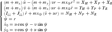(13)$$\left\{ \matrix{\left( {m + {m_x}} \right)\dot u - \left( {m + {m_y}} \right)vr - m{x_G}{r^2} = {X_H} + {X_P} + {X_R} \hfill \cr \left( {m + {m_y}} \right)\dot v + \left( {m + {m_x}} \right)ur + m{x_G}\dot r = {Y_H} + {Y_P} + {Y_R} \hfill \cr \left( {{I_{zz}} + {J_{zz}}} \right)\dot r + m{x_G}\left( {\dot v + ur} \right) = {N_H} + {N_P} + {N_R} \hfill \cr \dot \psi = r \hfill \cr {{\dot x}_0} = u\cos \psi - v\sin \psi \hfill \cr {{\dot y}_0} = v\cos \psi + u\sin \psi \hfill} \right.$$

Where the rudder servo system is also considered in the simulation, the steering engine is modelled as a system with single hydraulic circuit analogue control variable (Zhang, Reference Zhang2012), the maximum rudder ratio is ± 5^°/s and the saturation rudder angle is ± 35^°. u, v, r, ψ, x ₀, y ₀, n, δ denote linear and angular velocities, heading, positions, propeller rotational speed, rudder angle (expressed in rad) respectively; m and I _zz are the ship's mass and mass moment of inertia, respectively. m _x, m _y, J _zz are added mass and added moment of inertia. X _H, Y _H,N _H, X _P, Y _P, N _P, X _R, Y _R, N _R are hydrodynamic forces and moments acting on hull, propeller and rudder, respectively. For more details about the mathematical model, please refer to the references (Jia and Yang, Reference Jia and Yang1999; Fossen, Reference Fossen2011).

When the ship navigates at sea, the sway motion and heading deviation are caused mainly by marine environmental disturbances. In the simulation, one considers sea wind and irregular wind-generated waves. These are simulated by fusing the physical-based mathematical model. The wind speed (Beaufort No.7) V _wind = 14·25 m/s, wind direction ψ _wind = 85^°. The Joint North Sea Wave Project (JONSWAP) spectrum is adapted to produce the corresponding wind-related waves, which has been defined as an International Towing Tank Conference (ITTC) standard.

The simulation diagram implemented in Simulink is shown in Figure 3, the setting course is 50°. To provide quantification, three popular performance specifications, Equation (14) are employed to evaluate the corresponding algorithm. That is Mean Absolute Error (MAE), Mean Control Input (MCI) and the Total Variation (TV) of the control. MAE is used to measure the performance of the system response, and MCI and TV measure properties of energy consumption and smoothness. As to the nominal plant, the simulation results are presented in Figure 4. It is noted that the control effect of the nonlinear feedback driven by sine function is almost the same as that in the standard feedback (with the same maximum overshoot and settling time) while the initial maximum rudder angle is reduced to 24·02^° from the original 34·96^° with the drop of 31.2%. There is a 41.4% drop in the average rudder angle which is decreased on average to 0·0826^° from 0·1409^°. In order to illustrate the robust performance of the proposed algorithm, the perturbed plant is considered with the speed variation −50%. The corresponding response dynamics become worse than that of the nominal system. Figure 5 presents the simulation result for the perturbed condition. It is clear to note that saturation is generated in the initial stage using the standard feedback scheme but not under the nonlinear feedback scheme. The other performance indices of the nonlinear feedback scheme are still superior to that of the standard one. In Figures 4(b) and 5(b), the subfigure is a local zoom of the plot, which is to show the control dynamics clearly.

(14)$$\eqalign{& {\rm MAE} = \displaystyle{1 \over {{t_\infty} - {t_0}}}\int_{{t_0}}^{{t_\infty}} {\left \vert {r(t) - y(t)} \right \vert {\rm d}t}, \cr & {\rm MCI} = \displaystyle{1 \over {{t_\infty} - {t_0}}}\int_{{t_0}}^{{t_\infty}} {u(t){\rm d}t}, \cr & {\rm TV} = \displaystyle{1 \over {{t_\infty} - {t_0}}}\int_{{t_0}}^{{t_\infty}} {\left \vert {u(t + 1) - u(t)} \right \vert {\rm d}t}} $$

Figure 3.

Simulation diagram of Simulink.

Figure 4.

Simulation results for the nominal system: (a) System response, (b) Control input.

Figure 5.

Simulation results for the perturbed system: (a) System response, (b) Control input.

Table 1 gives a quantitative comparison of the simulation results, and this verifies the effectiveness of the nonlinear feedback algorithm. The performance specifications of MAE and MCI are approximated, the smoothness index of the control input is obviously lower than that of the standard feedback method. Under the circumstance of heavy sea state, steering with large rudder angles can increase the amplitude of roll and thus increase the probability of cargo damage and decrease the comfort index of seafarers as well as the safety coefficient of the ship. Therefore reducing the amplitude of rudder angle means that the ship will navigate more safely in addition to being more energy efficient.

Table 1.

Quantitative comparison of the simulation results.

In addition, Figure 6 gives the comparisons of the modulating functions N(e) = e, N(e) = ω ₁e and N(e) = sin (ω ₁e). As shown in Figure 6, it can be concluded that: the control performance of the nonlinear feedback N(e) = sin (ω ₁e) is equivalent to that of the linear feedback with an extra constant gain ω ₁ when the error e = r − y is small; the performance of the nonlinear feedback is superior to that of the linear feedback with an extra constant gain ω ₁ when the error e is medium; the nonlinear feedback technique cannot work effectively when the error e is too large. It is a very important conclusion that the improvement of control performance is at the cost of the reduction of the system robustness for both schemes by further simulation experiments.

Figure 6.

Comparison of the modulating functions (schematic diagram): N(e) = e, N(e) = ω ₁e and N(e) = sin (ω ₁e).