

1. Introduction
The Randolph Glacier Inventory (RGI) is a collection of digital outlines of the world’s glaciers, excluding the Greenland and Antarctic ice sheets. The RGI was developed in a short (1–2 year) period with limited resources in order to meet the needs of the Fifth Assessment Report (AR5) of the Intergovernmental Panel on Climate Change (IPCC) for estimates of recent and future glacier mass balance. Priority was given to complete coverage rather than to extensive documentary detail. The rationale of the RGI (Reference CaseyCasey, 2003; Reference CogleyCogley, 2009a; Reference OhmuraOhmura, 2009) is that fewer attributes and, if unavoidable, locally reduced accuracy of delineation (Section 3) would be a price worth paying for the complete coverage that is essential for global-scale assessments. However, of the few attributes attached to each RGI vector outline, some are analytically valuable. For example the terminus-type attribute and the complete coverage combine to yield the first estimate of the global proportion of tidewater glaciers.
Complete coverage is desirable for a broad range of global-scale investigations. Volume–area scaling (e.g. Reference Bahr, Meier and PeckhamBahr and others, 1997) and other procedures to derive glacier volume (e.g. Reference Farinotti, Huss, Bauder, Funk and TrufferFarinotti and others, 2009; Reference Linsbauer, Paul and HaeberliLinsbauer and others, 2012) require detailed knowledge of glacier areas, and in some cases a digital elevation model (DEM) as well. Glacier outlines are needed in geodetic estimation of volume changes by comparison of DEMs and altimetry, and of mass changes after the application of appropriate corrections (e.g. Reference Berthier, Schiefer, Menounos and RémyBerthier and others, 2010; Reference GardnerGardner and others, 2011). Glacier outlines are also crucial for the initialization of projections of glacier mass change (e.g. Reference Gregory and OerlemansGregory and Oerlemans, 1998; Reference Bahr, Dyurgerov and MeierBahr and others, 2009; Reference Marzeion, Jarosch and HoferMarzeion and others, 2012; Reference Radić, Bliss, Beedlow, Hock, Miles and CogleyRadić and others, 2014).
1.1 History
A global glacier inventory was first proposed, in the form of national lists of glaciers, during planning for the International Geophysical Year 1957–58. Progress was initially slow, but accelerated under the leadership of F. Müller during the 1970s, when the product became known as the World Glacier Inventory (WGI). The status of the WGI was assessed by the World Glacier Monitoring Service (Reference Haeberli, Bösch, Scherler, Østrem and WallénWGMS, 1989). A digital version has been available since 1995 from the National Snow and Ice Data Center (NSIDC), Boulder, Colorado, USA (http://nsidc.org/data/glacier_inventory/). It combined the WGI with the Eurasian Glacier Inventory of Reference Bedford and HaggertyBedford and Haggerty (1996) but still covered only ~25% of the global glacierized area. The extended WGI-XF inventory of Reference CogleyCogley (2009a) increased the global coverage to ~48%. Incompleteness aside, the WGI and its variants do not include glacier outlines, making them difficult to use for the global assessment of glacier change. A different initiative was launched in 1995 as GLIMS (Global Land Ice Measurements from Space). GLIMS, led initially by H.H. Kieffer and later by J.S. Kargel, is a consortium of regional investigators contributing glacier outlines in a digital vector format (Reference Raup and KhalsaRaup and others, 2007; Reference Kargel, Leonard, Bishop, Ka¨a¨b and RaupKargel and others, in press). The GLIMS inventory, which has an extensive set of attributes, has grown steadily, but it too remains incomplete. In mid-2013, its coverage was 58% of global glacierized area, although it has multitemporal coverage of several thousand glaciers.
Thus, half a century of work has yielded only two globally complete digital depictions of glacier extent: GGHYDRO (Reference CogleyCogley, 2003), a raster product compiled in the early 1980s, and the vectors of the Digital Chart of the World (DCW) of Reference DankoDanko (1992). Like DCW, GGHYDRO is highly generalized, but it has been used in several global-scale assessments (e.g. Reference Raper and BraithwaiteRaper and Braithwaite, 2006; Reference Hock, De Woul, Radić and DyurgerovHock and others, 2009; Reference Radić and HockRadić and Hock, 2010). Other assessments (e.g. Reference Meier and BahrMeier and Bahr, 1996; Reference Ohmura, Sparling and HawkesworthOhmura, 2004; Reference Dyurgerov and MeierDyurgerov and Meier, 2005; Reference Raper and BraithwaiteRaper and Braithwaite, 2005) have relied on separate indirect estimates of global aggregate information. Not all assessments have included the peripheral glaciers around the two ice sheets.
In recognition of the importance of baseline information for the assessment of glacier changes, the idea of a complete inventory of the world’s glaciers has been strongly endorsed by international organizations such as the World Meteorological Organization (2004).
Free access to the US Geological Survey’s archive of Landsat imagery (Reference Wulder, Masek, Cohen, Loveland and WoodcockWulder and others, 2012) has both stimulated and facilitated the mapping of glacier extent at regional and broader scales. The failure of the scan-line corrector of Landsat 7’s Enhanced Thematic Mapper Plus (ETM+) sensor in May 2003 (Reference Markham, Storey, Williams and IronsMarkham and others, 2004) limited the subsequent usefulness of that archive, but other sensors have offered a further stimulus by making possible, by stereographic or interferometric mapping, the construction of DEMs and thus the subdivision of ice bodies along drainage divides and the calculation of topographic and hypsometric glacier attributes. These products include the Advanced Spaceborne Thermal Emission and Reflection Radiometer (ASTER) global DEM and the DEM of the Shuttle Radar Topography Mission of February 2000. Their advantages and disadvantages are discussed by Reference Frey and PaulFrey and Paul (2012). In addition, several collaborative international projects, such as GlobGlacier (Reference Paul, Ka¨a¨b, Rott, Shepherd, Strozzi and VoldenPaul and others, 2009a) and Glaciers_cci (Reference Paul, Bolch, Ka¨a¨b, Nagler, Shepherd and StrozziPaul and others, 2012), have facilitated inventory-related data collection and production. Finally, the most immediate stimulus for rapid assembly of the RGI was the need for a globally complete inventory to meet the goals of the recently completed contribution of Working Group I to AR5 of the IPCC.
The RGI was planned by an ad hoc group that assembled four times between December 2010 and December 2011. One of the meeting venues, Randolph, New Hampshire, USA, gave its name to the resulting product. The members of the group pooled material already in their possession and approached other colleagues individually, and solicited additional contributions from the Cryolist (http://cryolist.org) and GLIMS communities and other sources. More than 60 colleagues from 18 countries contributed, making the RGI a truly global initiative.
1.2 Distribution of the RGI
The RGI is distributed through the GLIMS/NSIDC website (http://www.glims.org/RGI/randolph.html), and is accompanied by technical documentation (Reference ArendtArendt and others, 2013). To allow some contributors time to report their own results, access was initially granted on the understanding that the inventory be used only for purposes related to AR5. This constraint has now been removed. It is intended that in due course the RGI outlines will be merged into the GLIMS database. Planning of this merger is in progress (Reference Raup, Arendt, Armstrong, Barrett, Khalsa and RacoviteanuRaup and others, 2013).
The version described here, RGI 3.2, reflects the correction of topological, georeferencing and interpretative errors detected in RGI 1.0, released in February 2012, and RGI 2.0, released in June 2012, as well as the application of quality controls described in Section 2. Versions 3.0 and 3.1 were interim releases. Version 3.2 substitutes improved outlines in a number of regions, adds a small number of outlines from previously omitted regions, and features a uniform set of attributes (Section 2.4). Auxiliary information includes outlines of a set of 19 first-order and 89 second-order regions (see Section 2.3 and the Supplementary Information (http://www.igsoc.org/hyperlink/13j176/13j176supp.pdf) which includes maps showing the second-order regions).
2. Methods and Quality Control
2.1 Glacier outline generation and data sources
Parts of the RGI were compiled at several institutions, but the inventory was assembled in its entirety at the University of Alaska Fairbanks. The earliest version consisted of DCW outlines, which were then replaced by outlines from GLIMS where available. Further additions of new or replacement outlines from contributors were assimilated, checked and if necessary revised using standard vector-editing tools. All outlines were transformed when necessary to the World Geodetic System 1984 (WGS84) datum.
Most of the glacier outlines in the RGI with known dates were derived from satellite imagery acquired in 1999 or later. Various Landsat platforms, principally Landsat 5 TM and Landsat 7 ETM+, were the primary sources, and imagery from ASTER, IKONOS and SPOT 5 high-resolution stereo (HRS) sensors was also used. In northernmost Greenland, the RGI draws on the ice mask of the Greenland Mapping Project (Reference Howat, Negrete and SmithHowat and others, 2014). For most regions automatic or semi-automatic routines were used to map glaciers based on the distinctive spectral reflectance signatures of snow and ice in simple and normalized band-ratio maps (e.g. Reference Le Bris, Paul, Frey and BolchLe Bris and others, 2011). Some outlines were produced by manual digitizing on satellite imagery or on scanned digital copies of maps.
Glacier complexes (unsubdivided ice bodies) were subdivided into glaciers either by visual identification of flow divides or with semi-automated algorithms for detection of divides in a DEM (Reference Bolch, Menounos and WheateBolch and others, 2010; Reference Kienholz, Hock and ArendtKienholz and others, 2013). These algorithms use standard watershed delineation tools to build a preliminary map of ice ‘flowsheds’ which are then merged, based on chosen thresholds for the proximity of their termini, to form glaciers. The Bolch algorithm was applied in western Canada, parts of Alaska, Greenland and parts of High Mountain Asia. The Kienholz algorithm was developed, calibrated and quality-checked in Alaska and Arctic Canada South, and was applied without quality assessment in several other regions, where errors due to subdivision will be governed primarily by the quality of the DEM.
Some of our source inventories have been published only recently, including Reference NuthNuth and others (2013) for Svalbard, Reference Rastner, Bolch, Mölg, Machguth, Le Bris and PaulRastner and others (2012) for Greenland, and Reference Bliss, Hock and CogleyBliss and others (2013) for the Antarctic and Subantarctic. These three sources represent 5%, 12% and 18% of global glacier extent respectively. During assembly of the RGI, many GLIMS contributions of restricted extent were replaced by outlines from sources with more extensive coverage. However, the RGI outlines in British Columbia, the Caucasus and Iceland come entirely, and those in China mostly, from GLIMS, and there are also limited contributions in Central Asia and Alaska. GLIMS has therefore contributed at least 10% of the RGI coverage. The RGI still draws on the DCW for ~1% of global ice extent in northern Afghanistan, Tajikistan and Kyrgyzstan. In the Pyrenees, Iran and parts of North and Central Asia, the RGI records ‘nominal glaciers’ for which only location and area are available. They are represented by circles of the area reported in the WGI or WGI-XF, and account for <0.3% of global glacierized area. One glacierized region, Chukotka in easternmost Russia, does not appear in the RGI because the locations of its 17 km2 of glaciers (Reference SedovSedov, 1997) were unobtainable.
2.2 Outline geometry and topology
Each object in the RGI conforms to the data-model conventions of ESRI ArcGIS shapefiles. That is, each object consists of an outline encompassing the glacier, followed immediately by outlines representing all of its nunataks (ice-free areas enclosed by the glacier). This data model is not the same as the GLIMS data model, in which nunataks are independent objects.
Each component polygon of the RGI object is tested for closure, i.e. its last vertex is tested for identity with its first vertex. Polygons that are degenerate (having fewer than three distinct vertices) are removed. ArcGIS’s Repair Geometry tool is used to check correct ordering of points within each polygon. Overlapping polygons and small unassigned ‘sliver’ areas are corrected iteratively; they commonly result from the alteration of a glacier divide in only one of its two polygons. Scripts to run many of our topology checks are available at https://github.com/AGIScripts/script_glaciers.
Glaciers with areas less than 0.01 km2, the recommended minimum of the WGI, are removed. However, some of the source inventories had larger minimum-area thresholds, so not all regions include glaciers down to the 0.01 km2 threshold (Section 4.1). Nunataks are retained whatever their area. Glaciers contained within nunataks are recognized as independent ice bodies.
2.3 Regionalization
In regional or global studies it is convenient to group glaciers by proximity. Several different bases for regionalization can be imagined, such as grouping by climatological, hydro-graphic or topographic commonalities. However, no one scheme can serve all of the purposes for which a global glacier inventory might be used, and the RGI regions (Fig. 1) were developed under only three constraints: that they should resemble commonly recognized glacier domains, that together they should contain all of the world’s glaciers, and that their boundaries should be simple and readily recognizable on a map of the world.
First-order regions of the RGI, with glaciers shown in red. Region numbers are those of Table 2. Cylindrical equidistant projection.
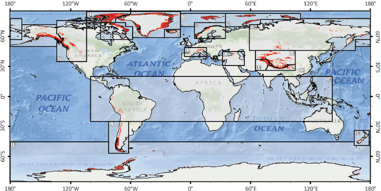
There are 19 first-order regions, derived from the regions of Reference Radić and HockRadić and Hock (2010) and modified in relatively minor ways. The first-order regions are subdivided into 89 second-order regions (http://www.igsoc.org/hyperlink/13j176/13j176supp.pdf: Table S1; Figs S1–S19). Most of the regional boundary segments follow parallels and meridians, but some adjacent regions are separated topographically along drainage divides. Widespread and consistent use of the RGI regions is encouraged as a way of facilitating comparisons between studies.
2.4 Attributes
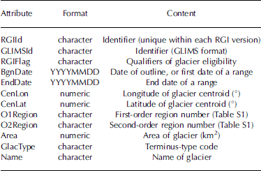
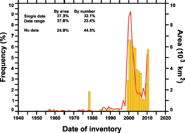
The RGI attaches 12 attributes, offering basic locational and identifying information, to each glacier (Tables 1 and S2). Each glacier has a unique RGIId code, a GLIMSId code (Reference Raup and KhalsaRaup and Khalsa, 2007) and, where it exists and is readily available, a Name. The RGIFlag attribute warns whether the glacier is a nominal glacier (Section 2.1) or a glacier complex (not yet subdivided from its neighbours, if any; this label appears only for 80 glaciers in the Low Latitudes). In Greenland, RGIFlag indicates which of three ‘connectivity levels’ (Reference Rastner, Bolch, Mölg, Machguth, Le Bris and PaulRastner and others, 2012) the glacier belongs to (Section 4.2), and in the Antarctic and Subantarctic, but not yet in other regions, it distinguishes between glaciers and ice caps. The GlacType attribute implements table 1 of Reference PaulPaul and others (2009b), although only the terminus-type code is assigned values (land-, marine-, lake- or shelf-terminating) in RGI 3.2. As yet, lake-terminating glaciers have been distinguished from land-terminating glaciers only in Alaska, the Southern Andes and Antarctica. First- and second-order region numbers are given by O1Region and O2Region. A more precise location is given by the longitude CenLon and latitude CenLat of the glacier; these attributes also appear in GLIMSId. Most of the locations are centroids of glacier polygons; ~1% lie outside their polygons. The glacier area is given by Area, which is calculated in Cartesian coordinates on a cylindrical equal-area projection of the authalic sphere of the WGS84 ellipsoid, or, for nominal glaciers, is accepted from the source inventory. The date of the source (Fig. 2) is given by BgnDate if it is known, or by a range BgnDate, EndDate. About 45% of the glaciers by number, accounting for 25% of global glacierized area, lack date information.
Glacier attributes in the Randolph Glacier Inventory. Further details are provided at http://www.igsoc.org/hyperlink/13j176/13j176supp.pdf
Frequency distribution of known dates and date ranges in the RGI by glacierized area (red line) and glacier number (yellow histogram). Glaciers with date ranges are assigned with uniform probability to each year of the range. Undated glaciers are not represented. Those in China date from the 1970s and 1980s and in Antarctica from the 1960s to 2000s. Most other undated glaciers are known to have been measured on Landsat ETM+, ASTER or SPOT5 imagery, i.e. of the late 1990s or later.
3. Accuracy
3.1 Data quality
Accurate recognition of glaciers in satellite imagery can be challenging (Reference PaulPaul and others, 2013). Maps can be similarly difficult to work with, and sometimes offer additional difficulties such as poor georeferencing and inadequate datum information. The accuracy of the result depends on the resolution and quality of the source imagery or map, the scale at which the analyst traces the glacier outlines, and his or her skill at identifying glacier surfaces consistently (e.g. Reference Bhambri and BolchBhambri and Bolch, 2009).
The glacier outlines in Figure 3 are from RGI 3.2 and are superimposed on Google Earth images. In each panel the outlines are of inadequate quality and need substantial reworking. Those in Figure 3a are at the correct locations, but many are too large by >50%. The outlines include ice-free glacier forefields, mountain rock walls, and rock glaciers. The outlines in Figure 3b are rather precise on the east side of the image and north of the drainage divide, but glaciers south of it and in the west are either missing, represented by nominal circles from the WGI, or digitized in a highly generalized way. In Figure 3c the outlines show some generalization, with missing nunataks, but the largest problem is the wrong geolocation. There is a systematic shift of all outlines relative to the satellite image in the background (which also shows seasonal snow cover, a potential cause of misinterpretation). Figure 3d illustrates the omission of many glaciers, and also outlines that are wrongly placed and highly generalized.
Images illustrating difficulties in the estimation of glacierized area for four regions in High Mountain Asia: (a) Hindu Kush, (b) northern Tien Shan, (c) Karakoram and (d) eastern Nyainqentanglha. All outlines are overlaid on Google Earth satellite images.
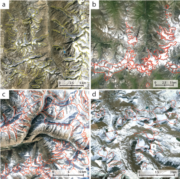
The problems illustrated here are addressed in Sections 3.2 and 3.3. Mislocated outlines have only limited effect on measurements of glacier area, but can introduce serious errors into procedures that rely on absolute positioning (e.g. co-registration to other datasets such as DEMs). Unless mislocations can be traced to systematic (and correctable) errors (e.g. due to misprojection or to errors in datum transformations), the only realistic way to correct them is to supply more accurate outlines. One highly anticipated source of improved outlines is the second Chinese Glacier Inventory.
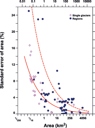
3.2 An error model
Because the sources of the RGI outlines are so diverse, it is not practical to estimate uncertainties source by source. Instead, we develop a simple model of uncertainty in glacier area, drawing on published estimates that have uncertainties attached. Small areas are harder to measure accurately than large areas (Fig. 4) because the measurement error tends to be inversely proportional to the length of the glacier margin. Estimates for collections of glaciers would ideally be calculated by summing the errors of glacier complexes rather than those of individual glaciers, because errors at flow divides sum to zero when both sides of the divide are included. However, Figure 4 shows no clear difference between single-glacier and multiple-glacier errors. We fit a power law by least squares to the relationship between fractional uncertainty and glacier area and assume as a first guess that this captures the contributions of inaccurate treatment of debris cover, omission of nunataks, inclusion of seasonal snow, and inaccurate mapping. This yields the relation
between the error e and area s (both in km2); p is 0.70, and e 1 = 0.039 is the estimated fractional error in a measured area of 1 km2. The correction factor k is discussed in Section 3.3. For each glacier in the RGI, the standard error is the arithmetic sum of e (s) as calculated for the glacier and all of its nunataks. Regional uncertainties presented below are also simple sums of all single-glacier area errors, which we expect, consistent with the simple reasoning that leads to Eqn (1), to be fully correlated.
Published estimates of the uncertainty of area measurements of single glaciers (diamonds) and collections of glaciers (dots). See http://www.igsoc.org/hyperlink/13j176/13j176supp.pdf for a list of sources. Solid line: best-fitting relationship between measured area and its standard error from Eqn (1) in text (with k = 1). Dashed line: relationship adopted for estimation of RGI errors (from Eqn (1) with k = 3).
3.3 A case study: South America
In earlier versions of the RGI, various factors obliged us to select satellite images of South America that in some cases showed extensive seasonal snow. Because it is time-consuming, the visual inspection needed to correct automatically generated outlines for the seasonal snow was not always possible. In RGI 3.2 we have corrected much of the resulting overestimate of glacier area by identifying images of better quality, but because seasonal snow was apparent in all available images our estimated ice cover in South America, 31 670 km2, may still be too large. There is no authoritative estimate for comparison; WGMS (1989) gives estimates for the South American nations which sum to 25 900 km2, but they are mostly undated and all involve some guesswork for unsurveyed regions.
We therefore assembled repeated measurements of the glacierized area of 37 South American subregions from the literature and compared them to corresponding sums of areas of RGI glaciers (Fig. 5). Where possible, we interpolated linearly from the bracketing dates of the independently measured areas from the literature to the date of the RGI image covering the subregion; where necessary, we extrapolated linearly, by from 0.5 to 9 years. (See www.igsoc.org/hyperlink/13j176/13j176supp.pdf for references.)
A comparison of RGI glacierized areas S for subregions in South America with equivalent measurements S ind from independent studies (listed at http://www.igsoc.org/hyperlink/13j176/13j176supp.pdf). The subregions, their approximate latitudes and independently obtained glacierized areas (km2) are listed at left. Orange dots: independent measurements (up to three per region); blue dots: averages of independent measurements (as listed at left, but uniformly zero in the graph); red crosses: RGI measurements (horizontal error bars are smaller than symbol size for most subregions).
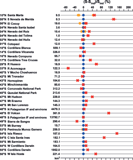
In five subregions where there are multiple independent measurements, the measurements differ, with standard deviations ranging from 1.2% to as great as 38%. After averaging these multiple measurements, the deviations ∆ = (S – S ind) /S ind between RGI areas S and independent areas S ind range from –68% (–63 km2) to +149% (+150 km2). The RGI total, 25 842 km2, is 5.4% greater than the independent total, 24 506 km2, and the mean and median of the absolute deviations | | are 30% and 13% respectively.
We conclude that area errors of tens of percent or more are possible in either or both of the RGI and the independent areas. Equation (1) (with k = 1) probably represents the best case, in which researchers have estimated uncertainties explicitly, although in a variety of ways. We are aware of further biases, due to one or more of the problems illustrated in Figure 3, in regions other than South America. For example, Reference Gardelle, Berthier, Arnaud and Ka¨a¨bGardelle and others (2013) found an average discrepancy in area of only –1.1% between RGI 2.0 and seven of their eight SPOT 5 scenes in South Asia, but in the eighth, in southeastern Tibet, RGI 2.0 has an extent 88% greater than their estimate. Many RGI contributions, notably in Alaska, Arctic Canada North and South, Greenland, Svalbard, the Russian Arctic, Central Europe and parts of South Asia West, are significantly more accurate than such worst-case examples. However, for the RGI as a whole we do not know how strongly the probability distribution of the errors is skewed by gross errors, so it seems prudent to scale Eqn (1), which captures an important part of the error structure, to reflect the likely non-normality of the error distribution. The sample of errors in Figure 4 and the sample of differences in Figure 5 both fail tests for goodness of fit to the normal distribution. Departures from normality are not surprising if we consider the difficulty of correcting for erratically variable seasonal snow, and equivalently the difficulty of recognizing debris-covered ice. It is also true that widely variable methods reduce the comparability of uncertainties estimated by different analysts.
How to correct Eqn (1) is not obvious, because the main sources of uncertainty, being heterogeneous across regions and data sources, are not amenable to handling with conventional statistics. Moreover, although Figure 5 suggests that Eqn (1) is likely to underestimate the uncertainty, a further consideration is that we have applied Eqn (1) to glaciers, rather than to glacier complexes as would be preferable because of the cancellation of errors at divides; a test calculation based on glacier complexes in the Russian Arctic yielded an area error of only ±1.2% as against ±2.8% for glaciers. As an interim measure pending further investigation, we set the correction factor k in Eqn (1) to 3 (a number chosen arbitrarily).
4. Results and Applications of the Inventory
4.1 Glacier numbers
The RGI contains outlines for ~198 000 glaciers. We stress that the total number of glaciers in the world, or in any region, is an arbitrary quantity. The fineness of subdivision of glacier complexes into glaciers varies from region to region, influenced by particular objectives and available resources. For example, glacier complexes in the Antarctic are subdivided less finely than elsewhere. Moreover, subdivision of ice bodies can produce doubtful results when the best available DEM or map is poor; glaciers tend to fragment in a warming climate; and the total number is strongly determined by the choice of minimum-area threshold (Reference Bahr and RadićBahr and Radić, 2012).
The spatial resolution of the source image or map will impose a minimum-area threshold for the identification of glaciers, but the choice of threshold is also influenced by the availability of resources. The labour needed for manual digitizing or for visual correction of automatically obtained outlines increases dramatically as the area threshold is reduced, and the time available for compiling a typical regional inventory can easily be overwhelmed by large numbers of very small glaciers. For example, in their glacier inventory of British Columbia (not part of the RGI), Reference Schiefer, Menounos and WheateSchiefer and others (2008) adopted a threshold of 0.1 km2 and an additional threshold based on glacier elevation ranges. By comparisons to subregional inventories with lower thresholds, they estimated that their thresholds excluded ~69% of the actual glaciers by number, but only ~7% of total glacierized area. In Section 4.2 we discuss the impact of omission of glaciers on the RGI estimates of glacier numbers and areas.
4.2 Glacier areas
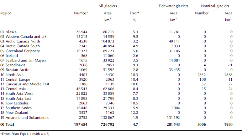
The total glacierized area in the RGI is 726 800 km2 (Table 2). The region with the most ice is the Antarctic and Subantarctic (132 900 km2), followed by Arctic Canada North with 104 900 km2. The regions with the least ice are the Caucasus and Middle East (1140 km2) and New Zealand (1160 km2). Of the total extent, 44% is in the Arctic regions (Arctic Canada North, Arctic Canada South, Greenland, Svalbard and Russian Arctic) and 18% in the Antarctic and Subantarctic. High Mountain Asia (i.e. Central Asia, South Asia West and South Asia East) accounts for 16% and Alaska for 12%. The uncertainty in total regional area depends on the distribution of glacier areas, which we discuss below. According to Eqn (1), regional uncertainty is as small as ±1.9% in the Antarctic and Subantarctic, where Reference Bliss, Hock and CogleyBliss and others (2013) assumed an uncertainty of ±5%, and exceeds ±10% in five regions with relatively small glaciers.
Summary of the RGI, Version 3.2
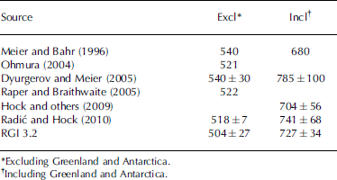
The total ice-covered area in RGI 3.2 is similar to earlier estimates (Table 3). Excluding Greenland and Antarctica, the largest deviation from the RGI in Table 3 is +7% (the areas determined by Reference Meier and BahrMeier and Bahr (1996) and Reference Dyurgerov and MeierDyurgerov and Meier (2005)), consistent with an uncertainty of the order of ±3.5%. The analysis in Section 3, however, suggests a somewhat greater uncertainty. The RGI area is the smallest of the entries. This is partly because some of the earlier estimates include 6000–8000 km2 of ice in the Subantarctic, which in the RGI is included in the Antarctic and Subantarctic region and thus excluded from this column of the table. Glacier shrinkage between older and newer sources of regional information may also account for some of the difference. When the Greenland and Antarctic glaciers are included, earlier estimates differ from the RGI by as much as –6% and +8%. These differences mainly reflect substantial improvement in the sources of information. Reference Rastner, Bolch, Mölg, Machguth, Le Bris and PaulRastner and others (2012) identified considerably more peripheral ice in Greenland than most previous investigations, and Reference Bliss, Hock and CogleyBliss and others (2013) relied mainly on the Antarctic Digital Database (ADD Consortium, 2000), a more accurate source than those of earlier estimates.
Published estimates of total glacierized area (103 km2)
Tidewater glaciers account for 39% of the total RGI extent. This statistic, reported earlier by Reference GardnerGardner and others (2013) using RGI 3.0, is valuable because it is the first entirely measurement-based estimate of the potential importance of tidewater glaciers among the world’s glaciers. It appears to confirm that the under-representation of calving glaciers and frontal ablation in mass-balance measurement programmes is more serious than calculated by Reference CogleyCogley (2009b), in whose dataset only 3% by area of the glaciers with glaciological measurements were tidewater glaciers. Including glaciers with geodetic measurements, the proportion rose to 16%, still well below the new RGI estimate.
In contrast to ice-sheet modelling, most modelling of glacier mass balance necessarily focuses on the climatic mass balance because the modelling of frontal losses due to dynamics is relatively underdeveloped, and more seriously because basic information required for the assessment of possible rapid dynamic responses of tidewater glaciers is only starting to be collected. Concrete evidence of rapid dynamic response is provided by Reference Burgess, Forster and LarsenBurgess and others (2013) for Alaska, where only 14% of the region’s glacier area is drained through tidewater outlets, but calving accounts for 36% of the regional loss rate. We expect that improved estimates of the extent of tidewater glaciers will aid in the determination of dynamical mass losses.
The proximity of glaciers in Greenland and Antarctica to the ice sheets requires care to avoid double-counting or omission by different groups working on large-scale cryospheric analyses. For example, gravimetric measurements of mass change by the Gravity Recovery and Climate Experiment (GRACE) satellites have low spatial resolution and are unable to distinguish the peripheral glaciers from the ice sheets. In Antarctica the implications of proximity are reduced, but not eliminated, because the RGI excludes the mainland. In Greenland the RGI includes all the peripheral glaciers, each of which is assigned a connectivity level CL (through RGIFlag; see Table S2 (http://www.igsoc.org/hyperlink/13j176/13j176supp.pdf)). The three values of CL represent glaciers that are unconnected, weakly connected or strongly connected to the ice sheet; the basis and methodology for these assignments are explained by Reference Rastner, Bolch, Mölg, Machguth, Le Bris and PaulRastner and others (2012). We follow their suggestion that the strongly connected CL2 glaciers, with an extent of 40 400 km2, be regarded as part of the Greenland ice sheet, yielding an area of 1 718 000 km2 for the ice sheet including the CL2 glaciers. (The CL2 glaciers are nevertheless included in the RGI shapefile for Greenland.) The areas of the CL0 (unconnected; 65 500 km2) and CL1 (weakly connected; 24 200 km2) glaciers sum to 89700 km2.
The frequency distribution of glacier areas is shown in Figure 6. Acknowledging that some very small glaciers may be omitted by virtue of the imposition of minimum-area thresholds, it is nevertheless clear that the area distribution is dominated by large glaciers. Glaciers with areas between ~4 and ~1500 km2 account for two-thirds of the ice cover.
Frequency distributions of glacier areas (histogram; left axis) and standard errors (connected dots; right axis). The continuous line shows the cumulative frequency distribution of areas (left axis, to be multiplied by 10).
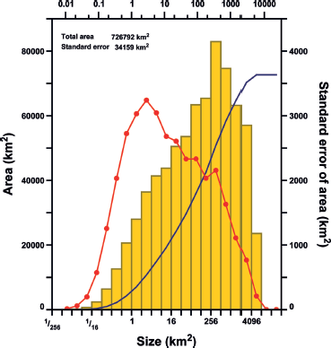
The distribution of standard errors in Figure 6 is based on Eqn (1) with k = 3 (Fig. 4). As follows from the form of Eqn (1) and the frequency distribution of the areas, smaller glaciers contribute more to the total uncertainty than do larger glaciers. In the smallest-size bin of Figure 6 the standard error of total bin area implied by Eqn (1) is 44%, while in the largest-size bin it is 0.9%. Of the uncertainty of 4.7% (34 000 km2) in the total area, two-thirds is contributed by glaciers with areas between ~1 and ~500 km2.
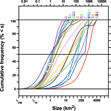
Figure 7 shows cumulative frequency distributions of glacier areas separated by first-order region. In seven regions the 50th percentile of the distribution (the ‘median area’) is smaller than 2 km2. The median area ranges upward to 181 km2 in Arctic Canada North, 351 km2 in Iceland and 706 km2 in Antarctica. In every region the mean area is con siderably less than the median area, reflecting the prominence of smaller glaciers in the size distribution of glacier numbers.
Cumulative frequency distributions of glacier areas for the RGI regions. Coloured numerals: region numbers (see Table 2). Open circles: percentiles of the mean glacier areas. Region numbers: 01. Alaska; 02. Western Canada and US; 03. Arctic Canada North; 04. Arctic Canada South; 05. Greenland Periphery; 06. Iceland; 07. Svalbard; 08. Scandinavia; 09. Russian Arctic; 10. North Asia; 11. Central Europe; 12. Caucasus and Middle East; 13. Central Asia; 14. South Asia West; 15. South Asia East; 16. Low Latitudes; 17. Southern Andes; 18. New Zealand; 19. Antarctic and Subantarctic.
With the possible exceptions of Central Europe and the Antarctic and Subantarctic, the regional size distributions of glacier numbers (Fig. 8) exhibit a common pattern in which numbers increase steeply from the smallest-size class towards a maximum, typically between 0.25 and 1 km2. Beyond this inflection, numbers decrease at a rate that varies little from region to region, with a tendency to steepen towards the largest-size class.
Size distributions of the number of glaciers for the RGI regions. Inset: an illustration of the argument for an upper bound on the RGI area (represented by the shaded region) that is missing due to the omission of glacierets.
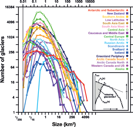
The inflection is due, to an unknown extent, to under-recording of glacierets and other very small glaciers, whether because of the imposition of a minimum-area threshold, or coarse DEM resolution, or for other reasons. Over-recording, by systematic misidentification of small (as opposed to large) snowpatches, is also possible. If we neglect this possibility because we are unable to quantify it, a lower bound on the underestimate due to under-recording is obtained by assuming that the RGI always distinguishes correctly between glacierets and snowpatches: no glacierets are omitted, and the underestimate is zero. An upper bound can be obtained by assuming that inverse power-law scaling, as suggested by the form of the size–frequency curves at larger sizes (Fig. 8), continues in reality down to the smallest sizes. For each region (inset of Fig. 8) we extrapolate the line connecting the most numerous class and its next larger neighbour, and sum the quantity S × [n× (S) – nRGI(S)] from the WGI minimum, s min = 0.01 km2, to sx , the size of the most numerous class. Here nx (s) is the extrapolated estimate of the ‘real’ number and n RGI(s) is the number of RGI glaciers of size s. The result is 10 180 km2 if we sum the 19 extrapolates, and 7819 km2 if we sum the regional glacier numbers and repeat the calculation for the entire world. Thus the underestimate of global total area due to omission of glacierets appears to lie between zero and an upper bound of 1.1–1.4%. The upper-bound calculations also imply a large increase in the total number of glaciers over that suggested in Section 4.1, to 462 000 for the region-by-region calculation and to 435 000 for the global calculation.
4.3 Glacier hypsometry
Among others (Reference Huss and FarinottiHuss and Farinotti, 2012; Reference Marzeion, Jarosch and HoferMarzeion and others, 2012), Reference Radić, Bliss, Beedlow, Hock, Miles and CogleyRadić and others (2014) have generated the hypsometry (area–altitude distribution) of each glacier from the RGI outlines and regional-scale DEMs. Figure 9a shows the total hypsometry of each region. Most of the world’s glacier area is below 2000 m, with comparatively little between 2500 m and 3500 m, where only Central Europe and the Caucasus and Middle East have hypsometric modes. The mid- and low-latitude glaciers of Central Asia, South Asia East, South Asia West and the Low Latitudes have most of their area above 4000 m. The spikes in the curves for Arctic Canada North, Arctic Canada South and Antarctica are DEM artefacts arising from poor interpolation from contour maps.
Area–elevation distributions of the RGI regions. (a) Distribution of regional glacierized area with elevation. (b) Distribution of normalized glacierized area with normalized elevation, with the idealized approximations of Reference Raper and BraithwaiteRaper and Braithwaite (2006) drawn as dotted lines (triangle for mountain glaciers, representative curved line for ice caps); the normalizations are explained in the text. Arctic Canada North and South, Greenland and the Russian Arctic (thick solid curves), and the Antarctic and Subantarctic (thick dashed curve), are discussed in the text.
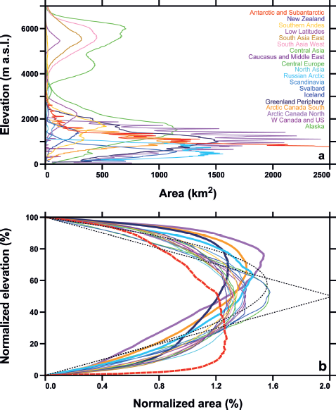
In Figure 9b, each glacier’s elevation range is normalized from 0 to 100 (i.e. its minimum elevation is set to 0 and its maximum to 100) and its total area is normalized to be equal to 100. Then all glaciers in each region are averaged without weighting, resulting in a typical, size-independent hypsometric curve for the glaciers of the region. These normalized, regionally averaged hypsometries exhibit three characteristic patterns. In most regions, most glaciers have most of their area in the middle of their elevation ranges, with less on steep high-elevation slopes and in narrow low-elevation tongues. In the Antarctic and Subantarctic, the predominance of tidewater glaciers skews the curve to lower normalized elevations. In Arctic Canada North, Arctic Canada South, the Russian Arctic and Greenland, the typical hypsometry is skewed to higher normalized elevations by ice caps on high-elevation plateaus with relatively restricted low-elevation tongues.
4.4 Glacier volume and mass
Working with WGI-XF (Reference CogleyCogley, 2009a), Radić and Hock (2010) produced an upscaled estimate, 600 ± 70 mm SLE (sea-level equivalent), of global glacier volume including glaciers around the ice sheets. This estimate was obtained by volume–area scaling (Reference Bahr, Meier and PeckhamBahr and others, 1997). One estimate relying on RGI 1.0, and three on RGI 2.0, have appeared recently (Table 4). Radić and others (2014) reduced the earlier Radić–Hock estimate to 522 mm SLE. Most of the reduction was ascribed to the availability of the RGI, which made upscaling unnecessary. An alternative assumption about the prevalence of ice caps, used by Radić and others (2014) as part of their assessment of uncertainty, made the global total lower still, at 405 mm SLE. Reference Marzeion, Jarosch and HoferMarzeion and others (2012), working with RGI 1.0, modelled regional ice volumes by volume–area scaling, but because they excluded glaciers in Antarctica the global total suggested in Table 4 for their work, 468 mm SLE, is a rough estimate and is not independent of the three other estimates. Reference Huss and FarinottiHuss and Farinotti (2012) estimated a total of 423 ± 57 mm SLE, based on a simple model of the glacier dynamics implied by the distribution of glacier surface elevations. Reference GrinstedGrinsted (2013), relying on a multivariate extension of volume–area scaling and on a different minimization criterion during calibration of the volume–area relationship, estimated a lesser total of 350 ± 70 mm SLE.
Glacier masses (Gt)* estimated with the RGI
The range of the estimates of total mass in Table 4 is 28% of their average (412 mm SLE). Explaining this spread is beyond the present scope, but some of the dispersion can be attributed to the rapid evolution of the RGI. For example, glaciers should not be aggregated for volume–area scaling, so glacier complexes, which were more numerous in RGI 1.0 and 2.0, dilute the accuracy of three of the estimates. Moreover, except in the Antarctic and Subantarctic, even RGI 3.2 offers no way to distinguish mountain and valley glaciers from ice caps. Volume–area scaling exponents for ice caps, whose thickness is large by comparison with the relief of their beds, are known to differ from those of mountain and valley glaciers (Reference Bahr, Meier and PeckhamBahr and others, 1997). The studies differed in their handling of this difference of scaling behaviour. The work of Huss and Farinotti may be less affected than the other three, although they noted that in Arctic Canada South, where separate sets of outlines were available for glaciers and glacier complexes, the total volume obtained by modelling the glaciers was 7% less than that obtained by modelling the complexes.
Reference Bahr and RadićBahr and Radić (2012) show that, for some purposes, glaciers in the smallest size classes of a given sample can contain a significant fraction of the total volume of the sample. They suggest that, at the global scale, an accuracy in volume of ±1% requires inclusion of all glaciers larger than 1 km2. At regional scales the threshold for a given desired accuracy depends on the size distribution. Where the largest glacier is of the order of 100 km2, total regional volume can only be estimated to ±10% or better if the minimum-area threshold is 0.01 km2 or smaller. In some regions, therefore, more accurate estimates of volume will require more complete inventories of the smallest glaciers.
4.5 Glacier climatology
Figure 10, less detailed versions of which have appeared in Reference Cogley, Henderson-Sellers and McGuffieCogley (2012) and Reference Huss and FarinottiHuss and Farinotti (2012), illustrates how a complete inventory can add value to information from other sources. The figure summarizes a wealth of glacio-climatic information, showing for example that at any latitude glaciers with lower mid-range altitudes tend to be warmer or more ‘maritime’. Maritime glaciers descend to lower altitudes than their more ‘continental’ counterparts, because more summer heat is required to remove the mass gained during their snowy winters. Conversely, continental glaciers tend to be dry and to persist only at higher, colder altitudes. Assuming that the mid-range altitude approximates the equilibrium-line altitude (which is not correct for tidewater glaciers), Figure 10 shows that the equilibrium line or snowline is not an isotherm: its temperature varies globally and at some single latitudes over a range of ~20ºC.
Zonal averages of the mean temperature of the warmest month at the glacier mid-range altitude (the average of the minimum and maximum glacier altitude). RGI glaciers with minimum altitudes of zero, assumed to be tidewater glaciers, were discarded. The mid-range altitude of each remaining glacier was estimated by overlaying its outline on a suitable DEM (see Reference Radić, Bliss, Beedlow, Hock, Miles and CogleyRadić and others, 2014, for details). The altitudes were averaged firstly into cells of size 50 m 0.58 0.58 and then over longitude. Temperatures are warmest-month free-air temperatures interpolated from the US National Centers for Environmental Prediction (NCEP)/National Center for Atmospheric Research (NCAR) Reanalysis (Reference KalnayKalnay and others, 1996).
Reference Mernild, Liston and HiemstraMernild and others (2013) extend the analysis shown in Figure 10. They use RGI glacier outlines to enable the modelling of Northern Hemisphere glacier freshwater balances driven by reanalysis data for annual time spans.
4.6 Evolution of glacier mass balance
Reference GardnerGardner and others (2013) used RGI 3.0 in the estimation of global average mass balance for 2003–09, a period for which estimates by interpolation of in situ measurements, satellite gravimetry and satellite laser altimetry are concurrently available. Results from in situ and remote-sensing methods differed significantly, but the RGI eliminated what was formerly the primary source of such differences, namely the previously differing estimates of regional glacier extent.
Reference Giesen and OerlemansGiesen and Oerlemans (2013) used RGI 1.0 to scale single-glacier mass-balance projections up to global scale over the 21st century, while Reference Hirabayashi, Zang, Watanabe, Koirala and KanaeHirabayashi and others (2013) used information derived from RGI 1.0 to simulate worldwide climatic mass balance from 1948 to 2099. Reference Marzeion, Jarosch and HoferMarzeion and others (2012) and Radić and others (2014) have published more detailed mass-balance modelling studies applied to each single RGI glacier, from versions 1.0 and 2.0 respectively. In each case the role of the RGI outline was to make possible the initialization of glacier area and hence volume, and the extraction of topography from a DEM. Both studies relied on the RGI regions as a standardized way to present geographical variations. Both were obliged to do their own subdivision of glacier complexes, and to generate topographic information by overlaying RGI outlines on DEMs. Marzeion and others, lacking dates for the outlines of RGI 1.0, had to supply them by intelligent guesswork. Radić and others accepted RGI 2.0, which has better but still incomplete date coverage, as a representation of ‘presentday’ glaciers. No global compilation of rates of area change is available, and it is therefore not yet possible to interpolate measured areas, even when their dates are known, to any particular reference date.
5. Summary and Outlook
The Randolph Glacier Inventory, a cooperative effort of the community of glaciologists, is a globally complete compilation of digital vector outlines of the world’s glaciers other than the ice sheets. It contains outlines of nearly 200 000 glaciers. Allowing for currently omitted glacierets the total number of glaciers could be greater, easily exceeding 400 000, but the missing glacierets represent 1.4% or less of the recorded glacierized area, and possibly much less. The total glacierized area is estimated as 726 800 ± 34 000 km2, although a number of questions remain about how best to calculate the uncertainty of this total. The area of glaciers on islands surrounding the Antarctic mainland is 132 900 ± 2520 km2 and the area of Greenland glaciers other than the ice sheet is 89 700 ± 4490 km2; the remaining glacierized regions contribute 504 200 ± 27 000 km2 to the total.
The RGI is a much richer product than the national lists envisaged half a century ago (Section 1.1), but is nevertheless a work in progress. Outstanding tasks include:
Improving the quality of outlines where recent regional inventories are likely to be more accurate. For example, recent work at the International Centre for Integrated Mountain Development, Kathmandu, Nepal (Reference Bajracharya and ShresthaBajracharya and Shrestha, 2011), and in China, is known to have better georeferencing and accuracy than RGI 3.2.
Providing outlines for ~3000 glaciers, mostly in North Asia, for which only location and area are known at present.
Shortening the time span of coverage. Of the outlines with dates, ~8% pre-date 1999.
Replacing date ranges with dates and supplying dates that are missing. Sometimes multiple images for a particular glacier make a range necessary, but many sources provide information in a form not readily converted to explicit dates.
Distinguishing between land-terminating and lake-terminating glaciers. So far, lake-terminating glaciers have been identified as such in only three regions.
Adding outlines of the debris-covered parts of glaciers.
Adding information about topography and hypsometry. Given the importance of early availability, it was decided not to try to include this information in the RGI. Several investigators have already exploited the RGI to retrieve detail from DEMs, but a standardized product (Reference PaulPaul and others, 2009b) of acknowledged uniform quality would reduce uncertainty arising from the use of different topographic sources, and would allow ice caps to be identified by examination of longitudinal profiles of surface elevation.
Documenting more completely the data sources and the methods used to delineate glaciers.
Merging the RGI into GLIMS. This is an organizational matter requiring forethought.
The RGI was not designed for the measurement of rates of glacier area change, for which the greatest possible accuracies in dating, delineation and georeferencing are essential. Many RGI outlines pass this test, but in general completeness of coverage had higher priority. Rather, the strength of the RGI lies in the capacity it offers for handling many glaciers at once (e.g. for estimating glacier volumes and rates of elevation change at regional and global scales and for simulating cryospheric responses to climatic forcing).
Finally, much remains to be done in the investigation of uncertainty. Our error model (Eqn (1)) incorporates some understanding of the sources of uncertainty, but does not address the non-normality of the errors arising from the diversity of information sources and methods of analysis. Further, the problem of uncertainty in glacier volume, at all scales from the single glacier to the world, is intractable. Measurements of volume are few, and understanding of the relationships between volume and the observable quantities is limited. Nevertheless uncertainty in glacier volume is a problem of wider significance than uncertainty in glacier area, and deserves continued attention.
Acknowledgements
We thank D. Bahr for helpful discussions, and an anonymous reviewer for a constructive review. Support for planning of the RGI, and for meetings in Winter Park, Colorado, and Randolph, New Hampshire, USA, was provided by the International Association for Cryospheric Sciences and the International Arctic Science Committee. K.M. Cuffey kindly provided the venue and helped to arrange a meeting in Berkeley, California, USA. We are grateful for support from NASA’s Cryospheric Research Branch (grants NNX11AF41G to C.K., NNX13AK37G to A.A. and J.R., NNX11AO23G to A.B.); the US Geological Survey’s Alaska Climate Science Center and the US National Park Service (grant H9911080028 to A.A. and J.R.); the European Space Agency (Glaciers_cci project 4000101778/10/I-AM to T.B. and F.P.); the ice2sea programme (European Union 7th Framework Programme grant No. 226375 to P.R.; ice2sea contribution No. 100); the German Research Foundation (DFG, grant BO 3199/2–1 to T.B.); the US National Science Foundation (grants ANT1043649 and EAR 0943742 to R.H.); the Austrian Science Fund (FWF; grants I900-N21 and P25362-N26 to G.K.); and the Natural Sciences and Engineering Research Council of Canada (Discovery Grant) and Environment Canada (to M.S.).
Appendix
Members of the Randolph Consortium
L.M. Andreassen,1 S. Bajracharya,2 N.E. Barrand,3 M.J. Beedle,4 E. Berthier,5 R. Bhambri,6 I. Brown,7 D.O. Burgess,8 E.W. Burgess,9 F. Cawkwell,10 T. Chinn,11 L. Copland,12 N.J. Cullen,13 B. Davies,14 H. De Angelis,7 A.G. Fountain,15 H. Frey,16 B.A. Giffen,17 N.F. Glasser,14 S.D. Gurney,18 W. Hagg,19 D.K. Hall,20 U.K. Haritashya,21 G. Hartmann,22 S. Herreid,9 I. Howat,23 H. Jiskoot,24 T.E. Khromova,25 A. Klein,26 J. Kohler,27 M. König,27 D. Kriegel,28 S. Kutuzov,25 I. Lavrentiev,25 R. Le Bris,16 X. Li,29 W.F. Manley,30 C. Mayer,31 B. Menounos,32 A. Mercer,7 P. Mool,2 A. Negrete,23 G. Nosenko,25 C. Nuth,33 A. Osmonov,34 R. Pettersson,35 A. Racoviteanu,36 R. Ranzi,37 M.A. Sarıkaya,38 C. Schneider,39 O. Sigurðsson,40 P. Sirguey,13 C.R. Stokes,41 R. Wheate,32 G.J. Wolken,42 L.Z. Wu,29 F.R. Wyatt43
-
1 Norwegian Water Resources and Energy Directorate, Oslo, Norway
-
2 International Centre for Integrated Mountain Development, Kathmandu, Nepal
-
3 University of Birmingham, Birmingham, UK
-
4 University of Northern British Columbia, Terrace, British Columbia, Canada
-
5 Laboratoire d'Etudes en Géophysique et Océanographie Spatiales, Toulouse, France
-
6 Wadia Institute of Himalayan Geology, Dehradun, India
-
7 Stockholm University, Stockholm, Sweden
-
8 Geological Survey of Canada, Ottawa, Ontario, Canada
-
9 University of Alaska Fairbanks, Fairbanks, AK, USA
-
10 University College Cork, Cork, Ireland
-
11 National Institute of Water and Atmospheric Research, Dunedin, New Zealand
-
12 University of Ottawa, Ottawa, Ontario, Canada
-
13 University of Otago, Dunedin, New Zealand
-
14 University of Aberystwyth, Aberystwyth, UK
-
15 Portland State University, Portland, OR, USA
-
16 University of Zürich, Zürich, Switzerland
-
17 National Park Service, Anchorage, AK, USA
-
18 University of Reading, Reading, UK
-
19 Ludwig Maximilians University, Munich, Germany
-
20 Goddard Space Flight Center, Greenbelt, MD, USA
-
21 University of Dayton, Dayton, OH, USA
-
22 Alberta Geological Survey, Edmonton, Alberta, Canada
-
23 The Ohio State University, Columbus, OH, USA
-
24 University of Lethbridge, Lethbridge, Alberta, Canada
-
25 Institute of Geography, Russian Academy of Sciences, Moscow, Russia
-
26 Texas A&M University, College Station, TX, USA
-
27 Norwegian Polar Institute, Tromsø, Norway
-
28 German Research Centre for Geosciences, Potsdam, Germany
-
29 Cold and Arid Regions Environmental and Engineering Research Institute, Lanzhou, China
-
30 University of Colorado, Boulder, CO, USA
-
31 Commission for Geodesy and Glaciology, Bavarian Academy of Sciences, Munich, Germany
-
32 University of Northern British Columbia, Prince George, British Columbia, Canada
-
33 University of Oslo, Oslo, Norway
-
34 Central Asian Institute of Applied Geosciences, Bishkek, Kyrgyzstan
-
35 University of Uppsala, Uppsala, Sweden
-
36 Laboratoire de Glaciologie et Géophysique de l'Environnement, Grenoble, France
-
37 University of Brescia, Brescia, Italy
-
38 Fatih University, Istanbul, Turkey
-
39 RWTH Aachen University, Aachen, Germany
-
40 Icelandic Meteorological Office, Reykjavík, Iceland
-
41 Durham University, Durham, UK
-
42 Alaska Division of Geological and Geophysical Surveys, Fairbanks, AK, USA
-
43 University of Alberta, Edmonton, Alberta, Canada


 Open access