


1. Introduction
Measurement invariance refers to the psychometric equivalence of an instrument (e.g., a questionnaire or test) across several specified groups, such as gender and ethnicity. The lack of measurement invariance suggests that the instrument has different structures or meanings to different groups, leading to biases in measurements (Millsap, Reference Millsap2012).
Measurement invariance is typically assessed by differential item functioning (DIF) analysis of item response data that aims to detect the measurement non-invariant items (i.e. DIF items). More precisely, a DIF item has a response distribution that depends on not only the latent trait measured by the instrument but also respondents’ group membership. Therefore, the detection of a DIF item involves comparing the item responses of different groups, conditioning on the latent traits. The complexity of the problem lies in that individuals’ latent trait levels cannot be directly observed but are measured by the instrument that may contain DIF items. In addition, different groups may have different latent trait distributions. This problem thus involves identifying the latent trait and then conducting the group comparison given individuals’ latent trait levels.
Many statistical methods have been developed for DIF analysis. Traditional methods for DIF analysis require prior knowledge about a set of DIF-free items, which is known as the anchor set. This anchor set is used to identify the latent trait distribution. These methods can be classified into two categories. Methods in the first category (Mantel and Haenszel, Reference Mantel and Haenszel1959; Dorans and Kulick, Reference Dorans and Kulick1986; Swaminathan and Rogers, Reference Swaminathan and Rogers1990; Shealy and Stout, Reference Shealy and Stout1993; Zwick et al., Reference Zwick, Thayer and Lewis2000; Zwick and Thayer, Reference Zwick and Thayer2002; May, Reference May2006; Soares et al., Reference Soares, Gonçalves and Gamerman2009; Frick et al., Reference Frick, Strobl and Zeileis2015) do not explicitly assume an item response theory (IRT) model, and methods in the second category (Thissen, Reference Thissen, Wainer and Braun1988; Lord, Reference Lord1980; Kim et al., Reference Kim, Cohen and Park1995; Raju, Reference Raju1988, Reference Raju1990; Woods et al., Reference Woods, Cai and Wang2013; Oort, Reference Oort1998; Steenkamp and Baumgartner, Reference Steenkamp and Baumgartner1998; Cao et al., Reference Cao, Tay and Liu2017; Woods et al., Reference Woods, Cai and Wang2013; Tay et al., Reference Tay, Meade and Cao2015, Reference Tay, Huang and Vermunt2016) are developed based on IRT models. Compared with non-IRT-based methods, an IRT-based method defines the DIF problem more clearly, at the price of potential model misspecification. Specifically, an IRT model represents the latent trait as a latent variable and further characterizes the item-specific DIF effects by modelling each item response distribution as a function of the latent variable and group membership.
The DIF problem is well-characterized by a multiple indicators, multiple causes (MIMIC) IRT model, which is a structural equation model originally developed for continuous indicators (Zellner, Reference Zellner1970; Goldberger, Reference Goldberger1972) and later extended to categorical item response data (Muthen, Reference Muthen1985; Muthen et al., Reference Muthen, Kao and Burstein1991; Muthen and Lehman, Reference Muthen and Lehman1985). A MIMIC model for DIF consists of a measurement component and a structural component. The measurement component models how the item responses depend on the measured psychological trait and respondents’ group membership. The structural component models the group-specific distributions of the psychological trait. The anchor set imposes zero constraints on item-specific parameters in the measurement component, making the model, including the latent trait distribution, identifiable. Consequently, the DIF effects of the rest of the items can be tested by drawing statistical inferences on the corresponding parameters under the identified model.
Anchor-set-based methods rely heavily on a correctly specified set of DIF-free items. The misspecification of some anchor items can lead to invalid statistical inference results – Type I errors increase and power decreases when anchor items are not completely DIF-free (Kopf et al., Reference Kopf, Zeileis and Strobl2015b). To address this issue, item purification methods (Candell and Drasgow, Reference Candell and Drasgow1988; Clauser et al., Reference Clauser, Mazor and Hambleton1993; Fidalgo et al., Reference Fidalgo, Mellenbergh and Muñiz2000; Wang and Yeh, Reference Wang and Yeh2003; Wang and Su, Reference Wang and Su2004; Wang et al., Reference Wang, Shih and Yang2009; Kopf et al., Reference Kopf, Zeileis and Strobl2015b, Reference Kopf, Zeileis and Strobla) have been proposed that iteratively select an anchor set by stepwise model selection methods. Several recently developed tree-based DIF detection methods (Strobl et al., Reference Strobl, Kopf and Zeileis2015; Tutz and Berger, Reference Tutz and Berger2016; Bollmann et al., Reference Bollmann, Berger and Tutz2018), which can detect DIF brought by continuous covariates, may be viewed as item purification methods. However, with multiple items containing DIF, item purification may suffer from masking and swamping effects (Barnett and Lewis, Reference Barnett and Lewis1994). More recently, regularized estimation methods (Magis et al., Reference Magis, Tuerlinckx and De Boeck2015; Tutz and Schauberger, Reference Tutz and Schauberger2015; Huang, Reference Huang2018; Belzak and Bauer, Reference Belzak and Bauer2020; Bauer et al., Reference Bauer, Belzak and Cole2020; Schauberger and Mair, Reference Schauberger and Mair2020) have been proposed that use LASSO-type regularized estimation procedures for simultaneous model selection and parameter estimation. Moreover, Bechger and Maris (Reference Bechger and Maris2015) proposed DIF detection methods based on the idea of differential item pair functioning, which does not require prior information about anchor items. Based on a similar idea as in Bechger and Maris (Reference Bechger and Maris2015), Yuan et al. (Reference Yuan, Liu and Han2021) proposed a relative change of difficulty difference method, in which data visualisation tools and Monte Carlo simulations are used to detect DIF items. Unfortunately, unlike many anchor-set-based methods with a correctly specified anchor set, these methods do not provide valid statistical inference for separately testing the null hypothesis of “item j is DIF-free” for each individual item j. Consequently, the type-I error for testing the hypothesis cannot be guaranteed to be controlled at a pre-specified significance level. For example, some item purification methods proceed by performing one or multiple hypothesis tests in each iteration, yielding some item-specific P-values. However, these tests are performed conditioning on the model previously selected, which fails to adjust for uncertainty in the iterative selection process (noting that the same data are used repeatedly). Consequently, the obtained P-values are not guaranteed to follow a uniform distribution, even in an asymptotic sense. Yuan et al. (Reference Yuan, Liu and Han2021) constructed confidence intervals for individual items. However, these confidence intervals are constructed by simulating from a setting where all the items are DIF-free. Consequently, they may not have the desired coverage or, equivalently, yield valid P-values for each individual item when there exist DIF items. Furthermore, although the regularised estimation methods have been shown to accurately detect DIF items, they are typically computationally intensive since they involve solving multiple regularized maximum likelihood estimation problems with different tuning parameters.
This paper proposes a new method that addresses the aforementioned issues with the existing methods. The proposed method can statistically accurately and computationally efficiently estimate the DIF effects without requiring prior knowledge about anchor items. It draws statistical inferences on the DIF effects of individual items, yielding valid confidence intervals and P-values. The point estimation and statistical inference lead to accurate detection of the DIF items, for which the item-level type-I error and further some test-level risk (e.g., false discovery rate) can be controlled by the inference results. The method is proposed under a MIMIC model with a two-parameter logistic (Birnbaum, Reference Birnbaum, Lord and Novick1968) IRT measurement model and a linear structural model. The key to this method is a minimal
\documentclass[12pt]{minimal}
\usepackage{amsmath}
\usepackage{wasysym}
\usepackage{amsfonts}
\usepackage{amssymb}
\usepackage{amsbsy}
\usepackage{mathrsfs}
\usepackage{upgreek}
\setlength{\oddsidemargin}{-69pt}
\begin{document}$$L_1$$\end{document}
 norm condition for identifying the true model. This condition assumes that the DIF effect parameters of the true model are sparse and, thus, imposes a sensible global structure on the measurement model. This structure can effectively identify the latent trait without knowing the anchor items and further detect the DIF items. As will be shown later, the minimal
\documentclass[12pt]{minimal}
\usepackage{amsmath}
\usepackage{wasysym}
\usepackage{amsfonts}
\usepackage{amssymb}
\usepackage{amsbsy}
\usepackage{mathrsfs}
\usepackage{upgreek}
\setlength{\oddsidemargin}{-69pt}
\begin{document}$$L_1$$\end{document}
norm condition for identifying the true model. This condition assumes that the DIF effect parameters of the true model are sparse and, thus, imposes a sensible global structure on the measurement model. This structure can effectively identify the latent trait without knowing the anchor items and further detect the DIF items. As will be shown later, the minimal
\documentclass[12pt]{minimal}
\usepackage{amsmath}
\usepackage{wasysym}
\usepackage{amsfonts}
\usepackage{amssymb}
\usepackage{amsbsy}
\usepackage{mathrsfs}
\usepackage{upgreek}
\setlength{\oddsidemargin}{-69pt}
\begin{document}$$L_1$$\end{document}
 norm condition holds when the proportion of non-DIF items is sufficiently large. Methods are developed for estimating the model parameters and obtaining confidence intervals and p-values, where the method for obtaining the confidence intervals and p-values can be viewed as a parametric bootstrap procedure (Davison and Hinkley, Reference Davison and Hinkley1997; Zhang, Reference Zhang2018). Procedures for the detection of DIF items are further developed. Our method is compared to the likelihood ratio test method (Thissen et al., Reference Thissen, Steinberg, Wainer, Holland and Wainer1993) that requires an anchor set, and a recently proposed LASSO-based approach (Belzak and Bauer, Reference Belzak and Bauer2020).
The rest of the paper is organised as follows: In Sect. 2, we introduce a MIMIC model framework for DIF analysis. Under this model framework, a new method is proposed for the statistical inference of DIF effects in Sect. 3. Related works are discussed in Sect. 4. Simulation studies and a real data application are given in Sects. 5 and 6, respectively. We conclude with discussions in Sect. 7. All the proofs for the proposition and theorems presented in the article, and the implementation details of the proposed algorithms can be found in the Supplementary Materials.
2. A MIMIC Formulation of DIF
Consider N individuals answering J items. Let
\documentclass[12pt]{minimal}
\usepackage{amsmath}
\usepackage{wasysym}
\usepackage{amsfonts}
\usepackage{amssymb}
\usepackage{amsbsy}
\usepackage{mathrsfs}
\usepackage{upgreek}
\setlength{\oddsidemargin}{-69pt}
\begin{document}$$Y_{ij} \in \{0, 1\}$$\end{document}
 be a binary random variable, denoting individual i’s response to item j. Let
\documentclass[12pt]{minimal}
\usepackage{amsmath}
\usepackage{wasysym}
\usepackage{amsfonts}
\usepackage{amssymb}
\usepackage{amsbsy}
\usepackage{mathrsfs}
\usepackage{upgreek}
\setlength{\oddsidemargin}{-69pt}
\begin{document}$$y_{ij}$$\end{document}
be a binary random variable, denoting individual i’s response to item j. Let
\documentclass[12pt]{minimal}
\usepackage{amsmath}
\usepackage{wasysym}
\usepackage{amsfonts}
\usepackage{amssymb}
\usepackage{amsbsy}
\usepackage{mathrsfs}
\usepackage{upgreek}
\setlength{\oddsidemargin}{-69pt}
\begin{document}$$y_{ij}$$\end{document}
 be the observed value, i.e., the realization, of
\documentclass[12pt]{minimal}
\usepackage{amsmath}
\usepackage{wasysym}
\usepackage{amsfonts}
\usepackage{amssymb}
\usepackage{amsbsy}
\usepackage{mathrsfs}
\usepackage{upgreek}
\setlength{\oddsidemargin}{-69pt}
\begin{document}$$Y_{ij}$$\end{document}
be the observed value, i.e., the realization, of
\documentclass[12pt]{minimal}
\usepackage{amsmath}
\usepackage{wasysym}
\usepackage{amsfonts}
\usepackage{amssymb}
\usepackage{amsbsy}
\usepackage{mathrsfs}
\usepackage{upgreek}
\setlength{\oddsidemargin}{-69pt}
\begin{document}$$Y_{ij}$$\end{document}
 . For the ease of exposition, we use
\documentclass[12pt]{minimal}
\usepackage{amsmath}
\usepackage{wasysym}
\usepackage{amsfonts}
\usepackage{amssymb}
\usepackage{amsbsy}
\usepackage{mathrsfs}
\usepackage{upgreek}
\setlength{\oddsidemargin}{-69pt}
\begin{document}$${\textbf{Y}}_i = (Y_{i1}, \ldots , Y_{iJ})$$\end{document}
. For the ease of exposition, we use
\documentclass[12pt]{minimal}
\usepackage{amsmath}
\usepackage{wasysym}
\usepackage{amsfonts}
\usepackage{amssymb}
\usepackage{amsbsy}
\usepackage{mathrsfs}
\usepackage{upgreek}
\setlength{\oddsidemargin}{-69pt}
\begin{document}$${\textbf{Y}}_i = (Y_{i1}, \ldots , Y_{iJ})$$\end{document}
 to denote the response vector of individual i. The individuals are from two groups, indicated by
\documentclass[12pt]{minimal}
\usepackage{amsmath}
\usepackage{wasysym}
\usepackage{amsfonts}
\usepackage{amssymb}
\usepackage{amsbsy}
\usepackage{mathrsfs}
\usepackage{upgreek}
\setlength{\oddsidemargin}{-69pt}
\begin{document}$$x_i = 0, 1$$\end{document}
to denote the response vector of individual i. The individuals are from two groups, indicated by
\documentclass[12pt]{minimal}
\usepackage{amsmath}
\usepackage{wasysym}
\usepackage{amsfonts}
\usepackage{amssymb}
\usepackage{amsbsy}
\usepackage{mathrsfs}
\usepackage{upgreek}
\setlength{\oddsidemargin}{-69pt}
\begin{document}$$x_i = 0, 1$$\end{document}
 , where 0 and 1 are referred to as the reference and focal groups, respectively. We further introduce a latent variable
\documentclass[12pt]{minimal}
\usepackage{amsmath}
\usepackage{wasysym}
\usepackage{amsfonts}
\usepackage{amssymb}
\usepackage{amsbsy}
\usepackage{mathrsfs}
\usepackage{upgreek}
\setlength{\oddsidemargin}{-69pt}
\begin{document}$$\theta _i$$\end{document}
, where 0 and 1 are referred to as the reference and focal groups, respectively. We further introduce a latent variable
\documentclass[12pt]{minimal}
\usepackage{amsmath}
\usepackage{wasysym}
\usepackage{amsfonts}
\usepackage{amssymb}
\usepackage{amsbsy}
\usepackage{mathrsfs}
\usepackage{upgreek}
\setlength{\oddsidemargin}{-69pt}
\begin{document}$$\theta _i$$\end{document}
 , which represents the latent trait that the items are designed to measure. DIF occurs when the distribution of
\documentclass[12pt]{minimal}
\usepackage{amsmath}
\usepackage{wasysym}
\usepackage{amsfonts}
\usepackage{amssymb}
\usepackage{amsbsy}
\usepackage{mathrsfs}
\usepackage{upgreek}
\setlength{\oddsidemargin}{-69pt}
\begin{document}$$\textbf{Y}_i$$\end{document}
, which represents the latent trait that the items are designed to measure. DIF occurs when the distribution of
\documentclass[12pt]{minimal}
\usepackage{amsmath}
\usepackage{wasysym}
\usepackage{amsfonts}
\usepackage{amssymb}
\usepackage{amsbsy}
\usepackage{mathrsfs}
\usepackage{upgreek}
\setlength{\oddsidemargin}{-69pt}
\begin{document}$$\textbf{Y}_i$$\end{document}
 depends on not only
\documentclass[12pt]{minimal}
\usepackage{amsmath}
\usepackage{wasysym}
\usepackage{amsfonts}
\usepackage{amssymb}
\usepackage{amsbsy}
\usepackage{mathrsfs}
\usepackage{upgreek}
\setlength{\oddsidemargin}{-69pt}
\begin{document}$$\theta _i$$\end{document}
depends on not only
\documentclass[12pt]{minimal}
\usepackage{amsmath}
\usepackage{wasysym}
\usepackage{amsfonts}
\usepackage{amssymb}
\usepackage{amsbsy}
\usepackage{mathrsfs}
\usepackage{upgreek}
\setlength{\oddsidemargin}{-69pt}
\begin{document}$$\theta _i$$\end{document}
 but also
\documentclass[12pt]{minimal}
\usepackage{amsmath}
\usepackage{wasysym}
\usepackage{amsfonts}
\usepackage{amssymb}
\usepackage{amsbsy}
\usepackage{mathrsfs}
\usepackage{upgreek}
\setlength{\oddsidemargin}{-69pt}
\begin{document}$$x_i$$\end{document}
but also
\documentclass[12pt]{minimal}
\usepackage{amsmath}
\usepackage{wasysym}
\usepackage{amsfonts}
\usepackage{amssymb}
\usepackage{amsbsy}
\usepackage{mathrsfs}
\usepackage{upgreek}
\setlength{\oddsidemargin}{-69pt}
\begin{document}$$x_i$$\end{document}
 . More precisely, DIF occurs if
\documentclass[12pt]{minimal}
\usepackage{amsmath}
\usepackage{wasysym}
\usepackage{amsfonts}
\usepackage{amssymb}
\usepackage{amsbsy}
\usepackage{mathrsfs}
\usepackage{upgreek}
\setlength{\oddsidemargin}{-69pt}
\begin{document}$${\textbf{Y}}_i$$\end{document}
. More precisely, DIF occurs if
\documentclass[12pt]{minimal}
\usepackage{amsmath}
\usepackage{wasysym}
\usepackage{amsfonts}
\usepackage{amssymb}
\usepackage{amsbsy}
\usepackage{mathrsfs}
\usepackage{upgreek}
\setlength{\oddsidemargin}{-69pt}
\begin{document}$${\textbf{Y}}_i$$\end{document}
 is not conditionally independent of
\documentclass[12pt]{minimal}
\usepackage{amsmath}
\usepackage{wasysym}
\usepackage{amsfonts}
\usepackage{amssymb}
\usepackage{amsbsy}
\usepackage{mathrsfs}
\usepackage{upgreek}
\setlength{\oddsidemargin}{-69pt}
\begin{document}$$x_i$$\end{document}
is not conditionally independent of
\documentclass[12pt]{minimal}
\usepackage{amsmath}
\usepackage{wasysym}
\usepackage{amsfonts}
\usepackage{amssymb}
\usepackage{amsbsy}
\usepackage{mathrsfs}
\usepackage{upgreek}
\setlength{\oddsidemargin}{-69pt}
\begin{document}$$x_i$$\end{document}
 , given
\documentclass[12pt]{minimal}
\usepackage{amsmath}
\usepackage{wasysym}
\usepackage{amsfonts}
\usepackage{amssymb}
\usepackage{amsbsy}
\usepackage{mathrsfs}
\usepackage{upgreek}
\setlength{\oddsidemargin}{-69pt}
\begin{document}$$\theta _i$$\end{document}
, given
\documentclass[12pt]{minimal}
\usepackage{amsmath}
\usepackage{wasysym}
\usepackage{amsfonts}
\usepackage{amssymb}
\usepackage{amsbsy}
\usepackage{mathrsfs}
\usepackage{upgreek}
\setlength{\oddsidemargin}{-69pt}
\begin{document}$$\theta _i$$\end{document}
 . Seemingly a simple group comparison problem, DIF analysis is non-trivial due to the latency of
\documentclass[12pt]{minimal}
\usepackage{amsmath}
\usepackage{wasysym}
\usepackage{amsfonts}
\usepackage{amssymb}
\usepackage{amsbsy}
\usepackage{mathrsfs}
\usepackage{upgreek}
\setlength{\oddsidemargin}{-69pt}
\begin{document}$$\theta _i$$\end{document}
. Seemingly a simple group comparison problem, DIF analysis is non-trivial due to the latency of
\documentclass[12pt]{minimal}
\usepackage{amsmath}
\usepackage{wasysym}
\usepackage{amsfonts}
\usepackage{amssymb}
\usepackage{amsbsy}
\usepackage{mathrsfs}
\usepackage{upgreek}
\setlength{\oddsidemargin}{-69pt}
\begin{document}$$\theta _i$$\end{document}
 . In particular, the distribution of
\documentclass[12pt]{minimal}
\usepackage{amsmath}
\usepackage{wasysym}
\usepackage{amsfonts}
\usepackage{amssymb}
\usepackage{amsbsy}
\usepackage{mathrsfs}
\usepackage{upgreek}
\setlength{\oddsidemargin}{-69pt}
\begin{document}$$\theta _i$$\end{document}
. In particular, the distribution of
\documentclass[12pt]{minimal}
\usepackage{amsmath}
\usepackage{wasysym}
\usepackage{amsfonts}
\usepackage{amssymb}
\usepackage{amsbsy}
\usepackage{mathrsfs}
\usepackage{upgreek}
\setlength{\oddsidemargin}{-69pt}
\begin{document}$$\theta _i$$\end{document}
 may depend on the value of
\documentclass[12pt]{minimal}
\usepackage{amsmath}
\usepackage{wasysym}
\usepackage{amsfonts}
\usepackage{amssymb}
\usepackage{amsbsy}
\usepackage{mathrsfs}
\usepackage{upgreek}
\setlength{\oddsidemargin}{-69pt}
\begin{document}$$x_i$$\end{document}
may depend on the value of
\documentclass[12pt]{minimal}
\usepackage{amsmath}
\usepackage{wasysym}
\usepackage{amsfonts}
\usepackage{amssymb}
\usepackage{amsbsy}
\usepackage{mathrsfs}
\usepackage{upgreek}
\setlength{\oddsidemargin}{-69pt}
\begin{document}$$x_i$$\end{document}
 , which confounds the DIF analysis. In what follows, we describe a MIMIC model framework for DIF analysis, under which the relationship among
\documentclass[12pt]{minimal}
\usepackage{amsmath}
\usepackage{wasysym}
\usepackage{amsfonts}
\usepackage{amssymb}
\usepackage{amsbsy}
\usepackage{mathrsfs}
\usepackage{upgreek}
\setlength{\oddsidemargin}{-69pt}
\begin{document}$${\textbf{Y}}_i$$\end{document}
, which confounds the DIF analysis. In what follows, we describe a MIMIC model framework for DIF analysis, under which the relationship among
\documentclass[12pt]{minimal}
\usepackage{amsmath}
\usepackage{wasysym}
\usepackage{amsfonts}
\usepackage{amssymb}
\usepackage{amsbsy}
\usepackage{mathrsfs}
\usepackage{upgreek}
\setlength{\oddsidemargin}{-69pt}
\begin{document}$${\textbf{Y}}_i$$\end{document}
 ,
\documentclass[12pt]{minimal}
\usepackage{amsmath}
\usepackage{wasysym}
\usepackage{amsfonts}
\usepackage{amssymb}
\usepackage{amsbsy}
\usepackage{mathrsfs}
\usepackage{upgreek}
\setlength{\oddsidemargin}{-69pt}
\begin{document}$$\theta _i$$\end{document}
,
\documentclass[12pt]{minimal}
\usepackage{amsmath}
\usepackage{wasysym}
\usepackage{amsfonts}
\usepackage{amssymb}
\usepackage{amsbsy}
\usepackage{mathrsfs}
\usepackage{upgreek}
\setlength{\oddsidemargin}{-69pt}
\begin{document}$$\theta _i$$\end{document}
 , and
\documentclass[12pt]{minimal}
\usepackage{amsmath}
\usepackage{wasysym}
\usepackage{amsfonts}
\usepackage{amssymb}
\usepackage{amsbsy}
\usepackage{mathrsfs}
\usepackage{upgreek}
\setlength{\oddsidemargin}{-69pt}
\begin{document}$$x_i$$\end{document}
, and
\documentclass[12pt]{minimal}
\usepackage{amsmath}
\usepackage{wasysym}
\usepackage{amsfonts}
\usepackage{amssymb}
\usepackage{amsbsy}
\usepackage{mathrsfs}
\usepackage{upgreek}
\setlength{\oddsidemargin}{-69pt}
\begin{document}$$x_i$$\end{document}
 is characterized. It is worth pointing out that this framework can be generalized to account for more complex DIF situations; see more details in Sect. 4.
2.1 Measurement Model
The two-parameter logistic (2PL) model (Birnbaum, Reference Birnbaum, Lord and Novick1968) is widely used to model binary item responses (e.g., wrong/right or absent/present). In the absence of DIF, the 2PL model assumes a logistic relationship between
\documentclass[12pt]{minimal}
\usepackage{amsmath}
\usepackage{wasysym}
\usepackage{amsfonts}
\usepackage{amssymb}
\usepackage{amsbsy}
\usepackage{mathrsfs}
\usepackage{upgreek}
\setlength{\oddsidemargin}{-69pt}
\begin{document}$$Y_{ij}$$\end{document}
 and
\documentclass[12pt]{minimal}
\usepackage{amsmath}
\usepackage{wasysym}
\usepackage{amsfonts}
\usepackage{amssymb}
\usepackage{amsbsy}
\usepackage{mathrsfs}
\usepackage{upgreek}
\setlength{\oddsidemargin}{-69pt}
\begin{document}$$\theta _i$$\end{document}
and
\documentclass[12pt]{minimal}
\usepackage{amsmath}
\usepackage{wasysym}
\usepackage{amsfonts}
\usepackage{amssymb}
\usepackage{amsbsy}
\usepackage{mathrsfs}
\usepackage{upgreek}
\setlength{\oddsidemargin}{-69pt}
\begin{document}$$\theta _i$$\end{document}
 , which is independent of the value of
\documentclass[12pt]{minimal}
\usepackage{amsmath}
\usepackage{wasysym}
\usepackage{amsfonts}
\usepackage{amssymb}
\usepackage{amsbsy}
\usepackage{mathrsfs}
\usepackage{upgreek}
\setlength{\oddsidemargin}{-69pt}
\begin{document}$$x_i$$\end{document}
, which is independent of the value of
\documentclass[12pt]{minimal}
\usepackage{amsmath}
\usepackage{wasysym}
\usepackage{amsfonts}
\usepackage{amssymb}
\usepackage{amsbsy}
\usepackage{mathrsfs}
\usepackage{upgreek}
\setlength{\oddsidemargin}{-69pt}
\begin{document}$$x_i$$\end{document}
 . That is,

where the slope parameter
\documentclass[12pt]{minimal}
\usepackage{amsmath}
\usepackage{wasysym}
\usepackage{amsfonts}
\usepackage{amssymb}
\usepackage{amsbsy}
\usepackage{mathrsfs}
\usepackage{upgreek}
\setlength{\oddsidemargin}{-69pt}
\begin{document}$$a_j$$\end{document}
 and intercept parameter
\documentclass[12pt]{minimal}
\usepackage{amsmath}
\usepackage{wasysym}
\usepackage{amsfonts}
\usepackage{amssymb}
\usepackage{amsbsy}
\usepackage{mathrsfs}
\usepackage{upgreek}
\setlength{\oddsidemargin}{-69pt}
\begin{document}$$d_j$$\end{document}
and intercept parameter
\documentclass[12pt]{minimal}
\usepackage{amsmath}
\usepackage{wasysym}
\usepackage{amsfonts}
\usepackage{amssymb}
\usepackage{amsbsy}
\usepackage{mathrsfs}
\usepackage{upgreek}
\setlength{\oddsidemargin}{-69pt}
\begin{document}$$d_j$$\end{document}
 are typically known as the discrimination and easiness parameters, respectively. The right-hand side of (1) as a function of
\documentclass[12pt]{minimal}
\usepackage{amsmath}
\usepackage{wasysym}
\usepackage{amsfonts}
\usepackage{amssymb}
\usepackage{amsbsy}
\usepackage{mathrsfs}
\usepackage{upgreek}
\setlength{\oddsidemargin}{-69pt}
\begin{document}$$\theta $$\end{document}
are typically known as the discrimination and easiness parameters, respectively. The right-hand side of (1) as a function of
\documentclass[12pt]{minimal}
\usepackage{amsmath}
\usepackage{wasysym}
\usepackage{amsfonts}
\usepackage{amssymb}
\usepackage{amsbsy}
\usepackage{mathrsfs}
\usepackage{upgreek}
\setlength{\oddsidemargin}{-69pt}
\begin{document}$$\theta $$\end{document}
 is known as the 2PL item response function. When the items potentially suffer from DIF, the item response functions may depend on the group membership
\documentclass[12pt]{minimal}
\usepackage{amsmath}
\usepackage{wasysym}
\usepackage{amsfonts}
\usepackage{amssymb}
\usepackage{amsbsy}
\usepackage{mathrsfs}
\usepackage{upgreek}
\setlength{\oddsidemargin}{-69pt}
\begin{document}$$x_i$$\end{document}
is known as the 2PL item response function. When the items potentially suffer from DIF, the item response functions may depend on the group membership
\documentclass[12pt]{minimal}
\usepackage{amsmath}
\usepackage{wasysym}
\usepackage{amsfonts}
\usepackage{amssymb}
\usepackage{amsbsy}
\usepackage{mathrsfs}
\usepackage{upgreek}
\setlength{\oddsidemargin}{-69pt}
\begin{document}$$x_i$$\end{document}
 . In that case, the item response function can be modelled as:

where
\documentclass[12pt]{minimal}
\usepackage{amsmath}
\usepackage{wasysym}
\usepackage{amsfonts}
\usepackage{amssymb}
\usepackage{amsbsy}
\usepackage{mathrsfs}
\usepackage{upgreek}
\setlength{\oddsidemargin}{-69pt}
\begin{document}$$\gamma _j$$\end{document}
 is an item-specific parameter that characterizes its DIF effect. More precisely,

That is,
\documentclass[12pt]{minimal}
\usepackage{amsmath}
\usepackage{wasysym}
\usepackage{amsfonts}
\usepackage{amssymb}
\usepackage{amsbsy}
\usepackage{mathrsfs}
\usepackage{upgreek}
\setlength{\oddsidemargin}{-69pt}
\begin{document}$$\exp (\gamma _j)$$\end{document}
 is the odds ratio for comparing two individuals from two groups who have the same latent trait level. Item j is DIF-free under this model when
\documentclass[12pt]{minimal}
\usepackage{amsmath}
\usepackage{wasysym}
\usepackage{amsfonts}
\usepackage{amssymb}
\usepackage{amsbsy}
\usepackage{mathrsfs}
\usepackage{upgreek}
\setlength{\oddsidemargin}{-69pt}
\begin{document}$$\gamma _j = 0$$\end{document}
is the odds ratio for comparing two individuals from two groups who have the same latent trait level. Item j is DIF-free under this model when
\documentclass[12pt]{minimal}
\usepackage{amsmath}
\usepackage{wasysym}
\usepackage{amsfonts}
\usepackage{amssymb}
\usepackage{amsbsy}
\usepackage{mathrsfs}
\usepackage{upgreek}
\setlength{\oddsidemargin}{-69pt}
\begin{document}$$\gamma _j = 0$$\end{document}
 . We further make the local independence assumption as in most IRT models. That is,
\documentclass[12pt]{minimal}
\usepackage{amsmath}
\usepackage{wasysym}
\usepackage{amsfonts}
\usepackage{amssymb}
\usepackage{amsbsy}
\usepackage{mathrsfs}
\usepackage{upgreek}
\setlength{\oddsidemargin}{-69pt}
\begin{document}$$Y_{i1}$$\end{document}
. We further make the local independence assumption as in most IRT models. That is,
\documentclass[12pt]{minimal}
\usepackage{amsmath}
\usepackage{wasysym}
\usepackage{amsfonts}
\usepackage{amssymb}
\usepackage{amsbsy}
\usepackage{mathrsfs}
\usepackage{upgreek}
\setlength{\oddsidemargin}{-69pt}
\begin{document}$$Y_{i1}$$\end{document}
 , ...,
\documentclass[12pt]{minimal}
\usepackage{amsmath}
\usepackage{wasysym}
\usepackage{amsfonts}
\usepackage{amssymb}
\usepackage{amsbsy}
\usepackage{mathrsfs}
\usepackage{upgreek}
\setlength{\oddsidemargin}{-69pt}
\begin{document}$$Y_{iJ}$$\end{document}
, ...,
\documentclass[12pt]{minimal}
\usepackage{amsmath}
\usepackage{wasysym}
\usepackage{amsfonts}
\usepackage{amssymb}
\usepackage{amsbsy}
\usepackage{mathrsfs}
\usepackage{upgreek}
\setlength{\oddsidemargin}{-69pt}
\begin{document}$$Y_{iJ}$$\end{document}
 are assumed to be conditionally independent, given
\documentclass[12pt]{minimal}
\usepackage{amsmath}
\usepackage{wasysym}
\usepackage{amsfonts}
\usepackage{amssymb}
\usepackage{amsbsy}
\usepackage{mathrsfs}
\usepackage{upgreek}
\setlength{\oddsidemargin}{-69pt}
\begin{document}$$\theta _i$$\end{document}
are assumed to be conditionally independent, given
\documentclass[12pt]{minimal}
\usepackage{amsmath}
\usepackage{wasysym}
\usepackage{amsfonts}
\usepackage{amssymb}
\usepackage{amsbsy}
\usepackage{mathrsfs}
\usepackage{upgreek}
\setlength{\oddsidemargin}{-69pt}
\begin{document}$$\theta _i$$\end{document}
 and
\documentclass[12pt]{minimal}
\usepackage{amsmath}
\usepackage{wasysym}
\usepackage{amsfonts}
\usepackage{amssymb}
\usepackage{amsbsy}
\usepackage{mathrsfs}
\usepackage{upgreek}
\setlength{\oddsidemargin}{-69pt}
\begin{document}$$x_i$$\end{document}
and
\documentclass[12pt]{minimal}
\usepackage{amsmath}
\usepackage{wasysym}
\usepackage{amsfonts}
\usepackage{amssymb}
\usepackage{amsbsy}
\usepackage{mathrsfs}
\usepackage{upgreek}
\setlength{\oddsidemargin}{-69pt}
\begin{document}$$x_i$$\end{document}
 .
.
2.2 Structural Model
A structural model specifies the distribution of
\documentclass[12pt]{minimal}
\usepackage{amsmath}
\usepackage{wasysym}
\usepackage{amsfonts}
\usepackage{amssymb}
\usepackage{amsbsy}
\usepackage{mathrsfs}
\usepackage{upgreek}
\setlength{\oddsidemargin}{-69pt}
\begin{document}$$\theta _i$$\end{document}
 , which may depend on the group membership. Specifically, we assume the conditional distribution of
\documentclass[12pt]{minimal}
\usepackage{amsmath}
\usepackage{wasysym}
\usepackage{amsfonts}
\usepackage{amssymb}
\usepackage{amsbsy}
\usepackage{mathrsfs}
\usepackage{upgreek}
\setlength{\oddsidemargin}{-69pt}
\begin{document}$$\theta _i$$\end{document}
, which may depend on the group membership. Specifically, we assume the conditional distribution of
\documentclass[12pt]{minimal}
\usepackage{amsmath}
\usepackage{wasysym}
\usepackage{amsfonts}
\usepackage{amssymb}
\usepackage{amsbsy}
\usepackage{mathrsfs}
\usepackage{upgreek}
\setlength{\oddsidemargin}{-69pt}
\begin{document}$$\theta _i$$\end{document}
 given
\documentclass[12pt]{minimal}
\usepackage{amsmath}
\usepackage{wasysym}
\usepackage{amsfonts}
\usepackage{amssymb}
\usepackage{amsbsy}
\usepackage{mathrsfs}
\usepackage{upgreek}
\setlength{\oddsidemargin}{-69pt}
\begin{document}$$x_i$$\end{document}
given
\documentclass[12pt]{minimal}
\usepackage{amsmath}
\usepackage{wasysym}
\usepackage{amsfonts}
\usepackage{amssymb}
\usepackage{amsbsy}
\usepackage{mathrsfs}
\usepackage{upgreek}
\setlength{\oddsidemargin}{-69pt}
\begin{document}$$x_i$$\end{document}
 to follow a normal distribution,

Note that the latent trait distribution for the reference group is set to a standard normal distribution to identify the location and scale of the latent trait. A similar assumption is typically adopted in IRT models for a single group of individuals.
The MIMIC model for DIF combines the above measurement and structural models, for which a path diagram is given in Fig. 1. The marginal likelihood function for this MIMIC model takes the form

where
\documentclass[12pt]{minimal}
\usepackage{amsmath}
\usepackage{wasysym}
\usepackage{amsfonts}
\usepackage{amssymb}
\usepackage{amsbsy}
\usepackage{mathrsfs}
\usepackage{upgreek}
\setlength{\oddsidemargin}{-69pt}
\begin{document}$$\Xi = \{\beta , \sigma ^2, a_j, d_j, \gamma _j, j = 1, \ldots , J\}$$\end{document}
 denotes all the fixed model parameters.
The goal of DIF analysis is to detect the DIF items, i.e., the items for which
\documentclass[12pt]{minimal}
\usepackage{amsmath}
\usepackage{wasysym}
\usepackage{amsfonts}
\usepackage{amssymb}
\usepackage{amsbsy}
\usepackage{mathrsfs}
\usepackage{upgreek}
\setlength{\oddsidemargin}{-69pt}
\begin{document}$$\gamma _j \ne 0$$\end{document}
 . Unfortunately, without further assumptions, this problem is ill-posed due to the non-identifiability of the model. We discuss this identifiability issue below.
The path diagram of a MIMIC model for DIF analysis. The subscript i is omitted for simplicity. The dashed lines from x to
\documentclass[12pt]{minimal}
\usepackage{amsmath}
\usepackage{wasysym}
\usepackage{amsfonts}
\usepackage{amssymb}
\usepackage{amsbsy}
\usepackage{mathrsfs}
\usepackage{upgreek}
\setlength{\oddsidemargin}{-69pt}
\begin{document}$$Y_j$$\end{document}
 indicate the DIF effects.

2.3 Model Identifiability
Without further assumptions, the above MIMIC model is not identifiable. That is, for any constant c, the model remains equivalent, if we simultaneously replace
\documentclass[12pt]{minimal}
\usepackage{amsmath}
\usepackage{wasysym}
\usepackage{amsfonts}
\usepackage{amssymb}
\usepackage{amsbsy}
\usepackage{mathrsfs}
\usepackage{upgreek}
\setlength{\oddsidemargin}{-69pt}
\begin{document}$$\beta $$\end{document}
 and
\documentclass[12pt]{minimal}
\usepackage{amsmath}
\usepackage{wasysym}
\usepackage{amsfonts}
\usepackage{amssymb}
\usepackage{amsbsy}
\usepackage{mathrsfs}
\usepackage{upgreek}
\setlength{\oddsidemargin}{-69pt}
\begin{document}$$\gamma _j$$\end{document}
and
\documentclass[12pt]{minimal}
\usepackage{amsmath}
\usepackage{wasysym}
\usepackage{amsfonts}
\usepackage{amssymb}
\usepackage{amsbsy}
\usepackage{mathrsfs}
\usepackage{upgreek}
\setlength{\oddsidemargin}{-69pt}
\begin{document}$$\gamma _j$$\end{document}
 by
\documentclass[12pt]{minimal}
\usepackage{amsmath}
\usepackage{wasysym}
\usepackage{amsfonts}
\usepackage{amssymb}
\usepackage{amsbsy}
\usepackage{mathrsfs}
\usepackage{upgreek}
\setlength{\oddsidemargin}{-69pt}
\begin{document}$$\beta +c$$\end{document}
by
\documentclass[12pt]{minimal}
\usepackage{amsmath}
\usepackage{wasysym}
\usepackage{amsfonts}
\usepackage{amssymb}
\usepackage{amsbsy}
\usepackage{mathrsfs}
\usepackage{upgreek}
\setlength{\oddsidemargin}{-69pt}
\begin{document}$$\beta +c$$\end{document}
 and
\documentclass[12pt]{minimal}
\usepackage{amsmath}
\usepackage{wasysym}
\usepackage{amsfonts}
\usepackage{amssymb}
\usepackage{amsbsy}
\usepackage{mathrsfs}
\usepackage{upgreek}
\setlength{\oddsidemargin}{-69pt}
\begin{document}$$\gamma _j -a_jc$$\end{document}
and
\documentclass[12pt]{minimal}
\usepackage{amsmath}
\usepackage{wasysym}
\usepackage{amsfonts}
\usepackage{amssymb}
\usepackage{amsbsy}
\usepackage{mathrsfs}
\usepackage{upgreek}
\setlength{\oddsidemargin}{-69pt}
\begin{document}$$\gamma _j -a_jc$$\end{document}
 , respectively, and keep
\documentclass[12pt]{minimal}
\usepackage{amsmath}
\usepackage{wasysym}
\usepackage{amsfonts}
\usepackage{amssymb}
\usepackage{amsbsy}
\usepackage{mathrsfs}
\usepackage{upgreek}
\setlength{\oddsidemargin}{-69pt}
\begin{document}$$a_j$$\end{document}
, respectively, and keep
\documentclass[12pt]{minimal}
\usepackage{amsmath}
\usepackage{wasysym}
\usepackage{amsfonts}
\usepackage{amssymb}
\usepackage{amsbsy}
\usepackage{mathrsfs}
\usepackage{upgreek}
\setlength{\oddsidemargin}{-69pt}
\begin{document}$$a_j$$\end{document}
 unchanged. This identifiability issue is due to that all the items are allowed to suffer from DIF, resulting in an unidentified latent trait. In other words, without further assumptions, it is impossible to disentangle the DIF effects and the difference between the latent trait distributions of the two groups.
According to Theorem 8.3 of San Martín (Reference San Martín and van der Linden2016), the location shift described above is the only source of indeterminacy for this MIMIC model when
\documentclass[12pt]{minimal}
\usepackage{amsmath}
\usepackage{wasysym}
\usepackage{amsfonts}
\usepackage{amssymb}
\usepackage{amsbsy}
\usepackage{mathrsfs}
\usepackage{upgreek}
\setlength{\oddsidemargin}{-69pt}
\begin{document}$$J\ge 3$$\end{document}
 and the sizes of both groups go to infinity. Let
\documentclass[12pt]{minimal}
\usepackage{amsmath}
\usepackage{wasysym}
\usepackage{amsfonts}
\usepackage{amssymb}
\usepackage{amsbsy}
\usepackage{mathrsfs}
\usepackage{upgreek}
\setlength{\oddsidemargin}{-69pt}
\begin{document}$$\Xi ^* = \{\beta ^*, (\sigma ^*)^2, a_j^*, d_j^*, \gamma _j^*, j = 1, \ldots , J\}$$\end{document}
and the sizes of both groups go to infinity. Let
\documentclass[12pt]{minimal}
\usepackage{amsmath}
\usepackage{wasysym}
\usepackage{amsfonts}
\usepackage{amssymb}
\usepackage{amsbsy}
\usepackage{mathrsfs}
\usepackage{upgreek}
\setlength{\oddsidemargin}{-69pt}
\begin{document}$$\Xi ^* = \{\beta ^*, (\sigma ^*)^2, a_j^*, d_j^*, \gamma _j^*, j = 1, \ldots , J\}$$\end{document}
 be a set of parameters for the true model. Then for any constant c, the set of parameters
\documentclass[12pt]{minimal}
\usepackage{amsmath}
\usepackage{wasysym}
\usepackage{amsfonts}
\usepackage{amssymb}
\usepackage{amsbsy}
\usepackage{mathrsfs}
\usepackage{upgreek}
\setlength{\oddsidemargin}{-69pt}
\begin{document}$$\Xi ^*(c) = \{\beta ^*+c, (\sigma ^*)^2, a_j^*, d_j^*, \gamma _j^* - a_j^*c, j = 1, \ldots , J\}$$\end{document}
be a set of parameters for the true model. Then for any constant c, the set of parameters
\documentclass[12pt]{minimal}
\usepackage{amsmath}
\usepackage{wasysym}
\usepackage{amsfonts}
\usepackage{amssymb}
\usepackage{amsbsy}
\usepackage{mathrsfs}
\usepackage{upgreek}
\setlength{\oddsidemargin}{-69pt}
\begin{document}$$\Xi ^*(c) = \{\beta ^*+c, (\sigma ^*)^2, a_j^*, d_j^*, \gamma _j^* - a_j^*c, j = 1, \ldots , J\}$$\end{document}
 gives the same data distribution. Moreover, if a set of parameters implies the same data distribution, then it has to take the form of
\documentclass[12pt]{minimal}
\usepackage{amsmath}
\usepackage{wasysym}
\usepackage{amsfonts}
\usepackage{amssymb}
\usepackage{amsbsy}
\usepackage{mathrsfs}
\usepackage{upgreek}
\setlength{\oddsidemargin}{-69pt}
\begin{document}$$\Xi ^*(c)$$\end{document}
gives the same data distribution. Moreover, if a set of parameters implies the same data distribution, then it has to take the form of
\documentclass[12pt]{minimal}
\usepackage{amsmath}
\usepackage{wasysym}
\usepackage{amsfonts}
\usepackage{amssymb}
\usepackage{amsbsy}
\usepackage{mathrsfs}
\usepackage{upgreek}
\setlength{\oddsidemargin}{-69pt}
\begin{document}$$\Xi ^*(c)$$\end{document}
 for some constant c. Knowing one or more anchor items means that the corresponding
\documentclass[12pt]{minimal}
\usepackage{amsmath}
\usepackage{wasysym}
\usepackage{amsfonts}
\usepackage{amssymb}
\usepackage{amsbsy}
\usepackage{mathrsfs}
\usepackage{upgreek}
\setlength{\oddsidemargin}{-69pt}
\begin{document}$$\gamma _j^*$$\end{document}
for some constant c. Knowing one or more anchor items means that the corresponding
\documentclass[12pt]{minimal}
\usepackage{amsmath}
\usepackage{wasysym}
\usepackage{amsfonts}
\usepackage{amssymb}
\usepackage{amsbsy}
\usepackage{mathrsfs}
\usepackage{upgreek}
\setlength{\oddsidemargin}{-69pt}
\begin{document}$$\gamma _j^*$$\end{document}
 s are known to be zero, which fixes the location indeterminacy. However, if no anchor item is known, we need to answer the question: which member of this equivalent class should be used to define DIF effects? We address it in Sect. 3.
3. Proposed Method
In what follows, we address the model identifiability problem raised above and then propose a new method for DIF analysis that does not require prior knowledge about anchor items under our definition of the true model parameters and additional regularity conditions. As will be shown in the rest, the proposed method can not only accurately detect the DIF items but also provide valid statistical inference for testing the hypotheses of
\documentclass[12pt]{minimal}
\usepackage{amsmath}
\usepackage{wasysym}
\usepackage{amsfonts}
\usepackage{amssymb}
\usepackage{amsbsy}
\usepackage{mathrsfs}
\usepackage{upgreek}
\setlength{\oddsidemargin}{-69pt}
\begin{document}$$\gamma _j = 0$$\end{document}
 , for any
\documentclass[12pt]{minimal}
\usepackage{amsmath}
\usepackage{wasysym}
\usepackage{amsfonts}
\usepackage{amssymb}
\usepackage{amsbsy}
\usepackage{mathrsfs}
\usepackage{upgreek}
\setlength{\oddsidemargin}{-69pt}
\begin{document}$$j = 1, \ldots , J$$\end{document}
, for any
\documentclass[12pt]{minimal}
\usepackage{amsmath}
\usepackage{wasysym}
\usepackage{amsfonts}
\usepackage{amssymb}
\usepackage{amsbsy}
\usepackage{mathrsfs}
\usepackage{upgreek}
\setlength{\oddsidemargin}{-69pt}
\begin{document}$$j = 1, \ldots , J$$\end{document}
 .
.
3.1 Model Identifiability, Sparsity, and Minimal
\documentclass[12pt]{minimal}
\usepackage{amsmath}
\usepackage{wasysym}
\usepackage{amsfonts}
\usepackage{amssymb}
\usepackage{amsbsy}
\usepackage{mathrsfs}
\usepackage{upgreek}
\setlength{\oddsidemargin}{-69pt}
\begin{document}$$L_1$$\end{document}
 Condition

We now address the model identifiability problem. The most natural idea is to choose
\documentclass[12pt]{minimal}
\usepackage{amsmath}
\usepackage{wasysym}
\usepackage{amsfonts}
\usepackage{amssymb}
\usepackage{amsbsy}
\usepackage{mathrsfs}
\usepackage{upgreek}
\setlength{\oddsidemargin}{-69pt}
\begin{document}$$\Xi ^*$$\end{document}
 as the true parameter vector when the corresponding
\documentclass[12pt]{minimal}
\usepackage{amsmath}
\usepackage{wasysym}
\usepackage{amsfonts}
\usepackage{amssymb}
\usepackage{amsbsy}
\usepackage{mathrsfs}
\usepackage{upgreek}
\setlength{\oddsidemargin}{-69pt}
\begin{document}$$\varvec{\gamma }^* = (\gamma _1^*, \ldots , \gamma _J^*)^\top $$\end{document}
as the true parameter vector when the corresponding
\documentclass[12pt]{minimal}
\usepackage{amsmath}
\usepackage{wasysym}
\usepackage{amsfonts}
\usepackage{amssymb}
\usepackage{amsbsy}
\usepackage{mathrsfs}
\usepackage{upgreek}
\setlength{\oddsidemargin}{-69pt}
\begin{document}$$\varvec{\gamma }^* = (\gamma _1^*, \ldots , \gamma _J^*)^\top $$\end{document}
 is the sparsest in the equivalent class
\documentclass[12pt]{minimal}
\usepackage{amsmath}
\usepackage{wasysym}
\usepackage{amsfonts}
\usepackage{amssymb}
\usepackage{amsbsy}
\usepackage{mathrsfs}
\usepackage{upgreek}
\setlength{\oddsidemargin}{-69pt}
\begin{document}$$\{\Xi ^*(c): c \in {\mathbb {R}}\}$$\end{document}
is the sparsest in the equivalent class
\documentclass[12pt]{minimal}
\usepackage{amsmath}
\usepackage{wasysym}
\usepackage{amsfonts}
\usepackage{amssymb}
\usepackage{amsbsy}
\usepackage{mathrsfs}
\usepackage{upgreek}
\setlength{\oddsidemargin}{-69pt}
\begin{document}$$\{\Xi ^*(c): c \in {\mathbb {R}}\}$$\end{document}
 . In other words, we say
\documentclass[12pt]{minimal}
\usepackage{amsmath}
\usepackage{wasysym}
\usepackage{amsfonts}
\usepackage{amssymb}
\usepackage{amsbsy}
\usepackage{mathrsfs}
\usepackage{upgreek}
\setlength{\oddsidemargin}{-69pt}
\begin{document}$$\Xi ^*$$\end{document}
. In other words, we say
\documentclass[12pt]{minimal}
\usepackage{amsmath}
\usepackage{wasysym}
\usepackage{amsfonts}
\usepackage{amssymb}
\usepackage{amsbsy}
\usepackage{mathrsfs}
\usepackage{upgreek}
\setlength{\oddsidemargin}{-69pt}
\begin{document}$$\Xi ^*$$\end{document}
 is the true model parameter when

for any
\documentclass[12pt]{minimal}
\usepackage{amsmath}
\usepackage{wasysym}
\usepackage{amsfonts}
\usepackage{amssymb}
\usepackage{amsbsy}
\usepackage{mathrsfs}
\usepackage{upgreek}
\setlength{\oddsidemargin}{-69pt}
\begin{document}$$c\ne 0$$\end{document}
 , where
\documentclass[12pt]{minimal}
\usepackage{amsmath}
\usepackage{wasysym}
\usepackage{amsfonts}
\usepackage{amssymb}
\usepackage{amsbsy}
\usepackage{mathrsfs}
\usepackage{upgreek}
\setlength{\oddsidemargin}{-69pt}
\begin{document}$$\varvec{\gamma }^*(c) = (\gamma _1^* - a_1^*c, \ldots , \gamma _J^* - a_J^*c)^\top $$\end{document}
, where
\documentclass[12pt]{minimal}
\usepackage{amsmath}
\usepackage{wasysym}
\usepackage{amsfonts}
\usepackage{amssymb}
\usepackage{amsbsy}
\usepackage{mathrsfs}
\usepackage{upgreek}
\setlength{\oddsidemargin}{-69pt}
\begin{document}$$\varvec{\gamma }^*(c) = (\gamma _1^* - a_1^*c, \ldots , \gamma _J^* - a_J^*c)^\top $$\end{document}
 and
\documentclass[12pt]{minimal}
\usepackage{amsmath}
\usepackage{wasysym}
\usepackage{amsfonts}
\usepackage{amssymb}
\usepackage{amsbsy}
\usepackage{mathrsfs}
\usepackage{upgreek}
\setlength{\oddsidemargin}{-69pt}
\begin{document}$$\Vert \cdot \Vert _0$$\end{document}
and
\documentclass[12pt]{minimal}
\usepackage{amsmath}
\usepackage{wasysym}
\usepackage{amsfonts}
\usepackage{amssymb}
\usepackage{amsbsy}
\usepackage{mathrsfs}
\usepackage{upgreek}
\setlength{\oddsidemargin}{-69pt}
\begin{document}$$\Vert \cdot \Vert _0$$\end{document}
 denotes the
\documentclass[12pt]{minimal}
\usepackage{amsmath}
\usepackage{wasysym}
\usepackage{amsfonts}
\usepackage{amssymb}
\usepackage{amsbsy}
\usepackage{mathrsfs}
\usepackage{upgreek}
\setlength{\oddsidemargin}{-69pt}
\begin{document}$$L_0$$\end{document}
denotes the
\documentclass[12pt]{minimal}
\usepackage{amsmath}
\usepackage{wasysym}
\usepackage{amsfonts}
\usepackage{amssymb}
\usepackage{amsbsy}
\usepackage{mathrsfs}
\usepackage{upgreek}
\setlength{\oddsidemargin}{-69pt}
\begin{document}$$L_0$$\end{document}
 norm, i.e., the number of nonzero entries in a vector. This definition requires the
\documentclass[12pt]{minimal}
\usepackage{amsmath}
\usepackage{wasysym}
\usepackage{amsfonts}
\usepackage{amssymb}
\usepackage{amsbsy}
\usepackage{mathrsfs}
\usepackage{upgreek}
\setlength{\oddsidemargin}{-69pt}
\begin{document}$$\varvec{\gamma }^*$$\end{document}
norm, i.e., the number of nonzero entries in a vector. This definition requires the
\documentclass[12pt]{minimal}
\usepackage{amsmath}
\usepackage{wasysym}
\usepackage{amsfonts}
\usepackage{amssymb}
\usepackage{amsbsy}
\usepackage{mathrsfs}
\usepackage{upgreek}
\setlength{\oddsidemargin}{-69pt}
\begin{document}$$\varvec{\gamma }^*$$\end{document}
 to be unique, which further implies that
\documentclass[12pt]{minimal}
\usepackage{amsmath}
\usepackage{wasysym}
\usepackage{amsfonts}
\usepackage{amssymb}
\usepackage{amsbsy}
\usepackage{mathrsfs}
\usepackage{upgreek}
\setlength{\oddsidemargin}{-69pt}
\begin{document}$$\Xi ^*$$\end{document}
to be unique, which further implies that
\documentclass[12pt]{minimal}
\usepackage{amsmath}
\usepackage{wasysym}
\usepackage{amsfonts}
\usepackage{amssymb}
\usepackage{amsbsy}
\usepackage{mathrsfs}
\usepackage{upgreek}
\setlength{\oddsidemargin}{-69pt}
\begin{document}$$\Xi ^*$$\end{document}
 is unique. We note that this sparsity assumption is essential if one wants to formulate the DIF detection problem as a model selection problem, i.e., using statistical criteria to decide which DIF effect parameters are zero. It is explicitly or implicitly made by most DIF detection methods that do not require anchor items, including item purification and regularised estimation methods. Note that our notion of true model parameter requires the true DIF parameter vector
\documentclass[12pt]{minimal}
\usepackage{amsmath}
\usepackage{wasysym}
\usepackage{amsfonts}
\usepackage{amssymb}
\usepackage{amsbsy}
\usepackage{mathrsfs}
\usepackage{upgreek}
\setlength{\oddsidemargin}{-69pt}
\begin{document}$$\varvec{\gamma }^*$$\end{document}
is unique. We note that this sparsity assumption is essential if one wants to formulate the DIF detection problem as a model selection problem, i.e., using statistical criteria to decide which DIF effect parameters are zero. It is explicitly or implicitly made by most DIF detection methods that do not require anchor items, including item purification and regularised estimation methods. Note that our notion of true model parameter requires the true DIF parameter vector
\documentclass[12pt]{minimal}
\usepackage{amsmath}
\usepackage{wasysym}
\usepackage{amsfonts}
\usepackage{amssymb}
\usepackage{amsbsy}
\usepackage{mathrsfs}
\usepackage{upgreek}
\setlength{\oddsidemargin}{-69pt}
\begin{document}$$\varvec{\gamma }^*$$\end{document}
 to have at least two zero elements, i.e.,
\documentclass[12pt]{minimal}
\usepackage{amsmath}
\usepackage{wasysym}
\usepackage{amsfonts}
\usepackage{amssymb}
\usepackage{amsbsy}
\usepackage{mathrsfs}
\usepackage{upgreek}
\setlength{\oddsidemargin}{-69pt}
\begin{document}$$\Vert \varvec{\gamma }^*\Vert _0 \le J-2$$\end{document}
to have at least two zero elements, i.e.,
\documentclass[12pt]{minimal}
\usepackage{amsmath}
\usepackage{wasysym}
\usepackage{amsfonts}
\usepackage{amssymb}
\usepackage{amsbsy}
\usepackage{mathrsfs}
\usepackage{upgreek}
\setlength{\oddsidemargin}{-69pt}
\begin{document}$$\Vert \varvec{\gamma }^*\Vert _0 \le J-2$$\end{document}
 . If
\documentclass[12pt]{minimal}
\usepackage{amsmath}
\usepackage{wasysym}
\usepackage{amsfonts}
\usepackage{amssymb}
\usepackage{amsbsy}
\usepackage{mathrsfs}
\usepackage{upgreek}
\setlength{\oddsidemargin}{-69pt}
\begin{document}$$\Vert \varvec{\gamma }^*\Vert _0 \ge J-1$$\end{document}
. If
\documentclass[12pt]{minimal}
\usepackage{amsmath}
\usepackage{wasysym}
\usepackage{amsfonts}
\usepackage{amssymb}
\usepackage{amsbsy}
\usepackage{mathrsfs}
\usepackage{upgreek}
\setlength{\oddsidemargin}{-69pt}
\begin{document}$$\Vert \varvec{\gamma }^*\Vert _0 \ge J-1$$\end{document}
 , then one can easily find a value of
\documentclass[12pt]{minimal}
\usepackage{amsmath}
\usepackage{wasysym}
\usepackage{amsfonts}
\usepackage{amssymb}
\usepackage{amsbsy}
\usepackage{mathrsfs}
\usepackage{upgreek}
\setlength{\oddsidemargin}{-69pt}
\begin{document}$$c\ne 0$$\end{document}
, then one can easily find a value of
\documentclass[12pt]{minimal}
\usepackage{amsmath}
\usepackage{wasysym}
\usepackage{amsfonts}
\usepackage{amssymb}
\usepackage{amsbsy}
\usepackage{mathrsfs}
\usepackage{upgreek}
\setlength{\oddsidemargin}{-69pt}
\begin{document}$$c\ne 0$$\end{document}
 such that
\documentclass[12pt]{minimal}
\usepackage{amsmath}
\usepackage{wasysym}
\usepackage{amsfonts}
\usepackage{amssymb}
\usepackage{amsbsy}
\usepackage{mathrsfs}
\usepackage{upgreek}
\setlength{\oddsidemargin}{-69pt}
\begin{document}$$\Vert \varvec{\gamma }^*(c)\Vert _0 \le \Vert \varvec{\gamma }^*\Vert _0$$\end{document}
such that
\documentclass[12pt]{minimal}
\usepackage{amsmath}
\usepackage{wasysym}
\usepackage{amsfonts}
\usepackage{amssymb}
\usepackage{amsbsy}
\usepackage{mathrsfs}
\usepackage{upgreek}
\setlength{\oddsidemargin}{-69pt}
\begin{document}$$\Vert \varvec{\gamma }^*(c)\Vert _0 \le \Vert \varvec{\gamma }^*\Vert _0$$\end{document}
 by setting
\documentclass[12pt]{minimal}
\usepackage{amsmath}
\usepackage{wasysym}
\usepackage{amsfonts}
\usepackage{amssymb}
\usepackage{amsbsy}
\usepackage{mathrsfs}
\usepackage{upgreek}
\setlength{\oddsidemargin}{-69pt}
\begin{document}$$c = \gamma _j^*/a_j^*$$\end{document}
by setting
\documentclass[12pt]{minimal}
\usepackage{amsmath}
\usepackage{wasysym}
\usepackage{amsfonts}
\usepackage{amssymb}
\usepackage{amsbsy}
\usepackage{mathrsfs}
\usepackage{upgreek}
\setlength{\oddsidemargin}{-69pt}
\begin{document}$$c = \gamma _j^*/a_j^*$$\end{document}
 for any j satisfying
\documentclass[12pt]{minimal}
\usepackage{amsmath}
\usepackage{wasysym}
\usepackage{amsfonts}
\usepackage{amssymb}
\usepackage{amsbsy}
\usepackage{mathrsfs}
\usepackage{upgreek}
\setlength{\oddsidemargin}{-69pt}
\begin{document}$$\gamma _j^* \ne 0$$\end{document}
for any j satisfying
\documentclass[12pt]{minimal}
\usepackage{amsmath}
\usepackage{wasysym}
\usepackage{amsfonts}
\usepackage{amssymb}
\usepackage{amsbsy}
\usepackage{mathrsfs}
\usepackage{upgreek}
\setlength{\oddsidemargin}{-69pt}
\begin{document}$$\gamma _j^* \ne 0$$\end{document}
 . In that case, the definition of
\documentclass[12pt]{minimal}
\usepackage{amsmath}
\usepackage{wasysym}
\usepackage{amsfonts}
\usepackage{amssymb}
\usepackage{amsbsy}
\usepackage{mathrsfs}
\usepackage{upgreek}
\setlength{\oddsidemargin}{-69pt}
\begin{document}$$\Xi ^*$$\end{document}
. In that case, the definition of
\documentclass[12pt]{minimal}
\usepackage{amsmath}
\usepackage{wasysym}
\usepackage{amsfonts}
\usepackage{amssymb}
\usepackage{amsbsy}
\usepackage{mathrsfs}
\usepackage{upgreek}
\setlength{\oddsidemargin}{-69pt}
\begin{document}$$\Xi ^*$$\end{document}
 is violated.
We also notice that the uniqueness of
\documentclass[12pt]{minimal}
\usepackage{amsmath}
\usepackage{wasysym}
\usepackage{amsfonts}
\usepackage{amssymb}
\usepackage{amsbsy}
\usepackage{mathrsfs}
\usepackage{upgreek}
\setlength{\oddsidemargin}{-69pt}
\begin{document}$$\varvec{\gamma }^*$$\end{document}
 is guaranteed when it is sufficiently sparse. In particular, when
\documentclass[12pt]{minimal}
\usepackage{amsmath}
\usepackage{wasysym}
\usepackage{amsfonts}
\usepackage{amssymb}
\usepackage{amsbsy}
\usepackage{mathrsfs}
\usepackage{upgreek}
\setlength{\oddsidemargin}{-69pt}
\begin{document}$$\Vert \varvec{\gamma }^*\Vert _0 < J/2$$\end{document}
is guaranteed when it is sufficiently sparse. In particular, when
\documentclass[12pt]{minimal}
\usepackage{amsmath}
\usepackage{wasysym}
\usepackage{amsfonts}
\usepackage{amssymb}
\usepackage{amsbsy}
\usepackage{mathrsfs}
\usepackage{upgreek}
\setlength{\oddsidemargin}{-69pt}
\begin{document}$$\Vert \varvec{\gamma }^*\Vert _0 < J/2$$\end{document}
 , then
\documentclass[12pt]{minimal}
\usepackage{amsmath}
\usepackage{wasysym}
\usepackage{amsfonts}
\usepackage{amssymb}
\usepackage{amsbsy}
\usepackage{mathrsfs}
\usepackage{upgreek}
\setlength{\oddsidemargin}{-69pt}
\begin{document}$$\Vert \varvec{\gamma }^*(c)\Vert _0 \ge J/2$$\end{document}
, then
\documentclass[12pt]{minimal}
\usepackage{amsmath}
\usepackage{wasysym}
\usepackage{amsfonts}
\usepackage{amssymb}
\usepackage{amsbsy}
\usepackage{mathrsfs}
\usepackage{upgreek}
\setlength{\oddsidemargin}{-69pt}
\begin{document}$$\Vert \varvec{\gamma }^*(c)\Vert _0 \ge J/2$$\end{document}
 for any
\documentclass[12pt]{minimal}
\usepackage{amsmath}
\usepackage{wasysym}
\usepackage{amsfonts}
\usepackage{amssymb}
\usepackage{amsbsy}
\usepackage{mathrsfs}
\usepackage{upgreek}
\setlength{\oddsidemargin}{-69pt}
\begin{document}$$c\ne 0$$\end{document}
for any
\documentclass[12pt]{minimal}
\usepackage{amsmath}
\usepackage{wasysym}
\usepackage{amsfonts}
\usepackage{amssymb}
\usepackage{amsbsy}
\usepackage{mathrsfs}
\usepackage{upgreek}
\setlength{\oddsidemargin}{-69pt}
\begin{document}$$c\ne 0$$\end{document}
 (assuming that
\documentclass[12pt]{minimal}
\usepackage{amsmath}
\usepackage{wasysym}
\usepackage{amsfonts}
\usepackage{amssymb}
\usepackage{amsbsy}
\usepackage{mathrsfs}
\usepackage{upgreek}
\setlength{\oddsidemargin}{-69pt}
\begin{document}$$a_j^* \ne 0$$\end{document}
(assuming that
\documentclass[12pt]{minimal}
\usepackage{amsmath}
\usepackage{wasysym}
\usepackage{amsfonts}
\usepackage{amssymb}
\usepackage{amsbsy}
\usepackage{mathrsfs}
\usepackage{upgreek}
\setlength{\oddsidemargin}{-69pt}
\begin{document}$$a_j^* \ne 0$$\end{document}
 for all j), and thus, the uniqueness of
\documentclass[12pt]{minimal}
\usepackage{amsmath}
\usepackage{wasysym}
\usepackage{amsfonts}
\usepackage{amssymb}
\usepackage{amsbsy}
\usepackage{mathrsfs}
\usepackage{upgreek}
\setlength{\oddsidemargin}{-69pt}
\begin{document}$$\varvec{\gamma }^*$$\end{document}
for all j), and thus, the uniqueness of
\documentclass[12pt]{minimal}
\usepackage{amsmath}
\usepackage{wasysym}
\usepackage{amsfonts}
\usepackage{amssymb}
\usepackage{amsbsy}
\usepackage{mathrsfs}
\usepackage{upgreek}
\setlength{\oddsidemargin}{-69pt}
\begin{document}$$\varvec{\gamma }^*$$\end{document}
 is guaranteed. In the rest, we consider settings when
\documentclass[12pt]{minimal}
\usepackage{amsmath}
\usepackage{wasysym}
\usepackage{amsfonts}
\usepackage{amssymb}
\usepackage{amsbsy}
\usepackage{mathrsfs}
\usepackage{upgreek}
\setlength{\oddsidemargin}{-69pt}
\begin{document}$$\varvec{\gamma }^*$$\end{document}
is guaranteed. In the rest, we consider settings when
\documentclass[12pt]{minimal}
\usepackage{amsmath}
\usepackage{wasysym}
\usepackage{amsfonts}
\usepackage{amssymb}
\usepackage{amsbsy}
\usepackage{mathrsfs}
\usepackage{upgreek}
\setlength{\oddsidemargin}{-69pt}
\begin{document}$$\varvec{\gamma }^*$$\end{document}
 is sufficiently sparse. Further discussions will be provided in the sequel regarding the sparsity level. We note that this “sufficiently sparse" assumption aligns well with the practical utility of DIF analysis in educational testing (e.g., Holland & Wainer, Reference Holland and Wainer1993) as well as certain settings of psychological measurement (e.g., Chapter 1, Millsap, Reference Millsap2012) and health-related measurement (e.g., Scott et al., Reference Scott, Fayers, Aaronson, Bottomley, de Graeff, Groenvold, Gundy, Koller, Petersen and Sprangers2010). For example, in educational testing, DIF analysis is conducted to ensure the fairness of a test form. In this application, the test operator aims to identify a small number of DIF items that cause a bias in the test result. The identified items will be reviewed by domain experts and then revised or removed from the item pool. For this process to be operationally feasible, one typically needs to assume that most items are DIF-free, i.e.,
\documentclass[12pt]{minimal}
\usepackage{amsmath}
\usepackage{wasysym}
\usepackage{amsfonts}
\usepackage{amssymb}
\usepackage{amsbsy}
\usepackage{mathrsfs}
\usepackage{upgreek}
\setlength{\oddsidemargin}{-69pt}
\begin{document}$$\varvec{\gamma }^*$$\end{document}
is sufficiently sparse. Further discussions will be provided in the sequel regarding the sparsity level. We note that this “sufficiently sparse" assumption aligns well with the practical utility of DIF analysis in educational testing (e.g., Holland & Wainer, Reference Holland and Wainer1993) as well as certain settings of psychological measurement (e.g., Chapter 1, Millsap, Reference Millsap2012) and health-related measurement (e.g., Scott et al., Reference Scott, Fayers, Aaronson, Bottomley, de Graeff, Groenvold, Gundy, Koller, Petersen and Sprangers2010). For example, in educational testing, DIF analysis is conducted to ensure the fairness of a test form. In this application, the test operator aims to identify a small number of DIF items that cause a bias in the test result. The identified items will be reviewed by domain experts and then revised or removed from the item pool. For this process to be operationally feasible, one typically needs to assume that most items are DIF-free, i.e.,
\documentclass[12pt]{minimal}
\usepackage{amsmath}
\usepackage{wasysym}
\usepackage{amsfonts}
\usepackage{amssymb}
\usepackage{amsbsy}
\usepackage{mathrsfs}
\usepackage{upgreek}
\setlength{\oddsidemargin}{-69pt}
\begin{document}$$\varvec{\gamma }^*$$\end{document}
 is sufficiently sparse.
The
\documentclass[12pt]{minimal}
\usepackage{amsmath}
\usepackage{wasysym}
\usepackage{amsfonts}
\usepackage{amssymb}
\usepackage{amsbsy}
\usepackage{mathrsfs}
\usepackage{upgreek}
\setlength{\oddsidemargin}{-69pt}
\begin{document}$$L_0$$\end{document}
 norm is not easy to work with from a statistical perspective. Due to the randomness in the data, likelihood-based estimation methods almost never give us a truly sparse solution. Consequently, one essentially needs to search over
\documentclass[12pt]{minimal}
\usepackage{amsmath}
\usepackage{wasysym}
\usepackage{amsfonts}
\usepackage{amssymb}
\usepackage{amsbsy}
\usepackage{mathrsfs}
\usepackage{upgreek}
\setlength{\oddsidemargin}{-69pt}
\begin{document}$$O(2^J)$$\end{document}
norm is not easy to work with from a statistical perspective. Due to the randomness in the data, likelihood-based estimation methods almost never give us a truly sparse solution. Consequently, one essentially needs to search over
\documentclass[12pt]{minimal}
\usepackage{amsmath}
\usepackage{wasysym}
\usepackage{amsfonts}
\usepackage{amssymb}
\usepackage{amsbsy}
\usepackage{mathrsfs}
\usepackage{upgreek}
\setlength{\oddsidemargin}{-69pt}
\begin{document}$$O(2^J)$$\end{document}
 all possible models to find the sparest model (e.g., using a suitable information criterion). Item purification and regularized estimation methods narrow the search by stepwise procedures and regularized estimation procedures, respectively. Even with these methods, the computation can still be intensive, and consistent selection of the true model is not always guaranteed.
To develop our method, we consider a surrogate to (4). Specifically, we require the following minimal
\documentclass[12pt]{minimal}
\usepackage{amsmath}
\usepackage{wasysym}
\usepackage{amsfonts}
\usepackage{amssymb}
\usepackage{amsbsy}
\usepackage{mathrsfs}
\usepackage{upgreek}
\setlength{\oddsidemargin}{-69pt}
\begin{document}$$L_1$$\end{document}
 (ML1) condition to hold

or equivalently,
\documentclass[12pt]{minimal}
\usepackage{amsmath}
\usepackage{wasysym}
\usepackage{amsfonts}
\usepackage{amssymb}
\usepackage{amsbsy}
\usepackage{mathrsfs}
\usepackage{upgreek}
\setlength{\oddsidemargin}{-69pt}
\begin{document}$$\Vert \varvec{\gamma }^*\Vert _1 < \Vert \varvec{\gamma }^*(c)\Vert _1$$\end{document}
 for all
\documentclass[12pt]{minimal}
\usepackage{amsmath}
\usepackage{wasysym}
\usepackage{amsfonts}
\usepackage{amssymb}
\usepackage{amsbsy}
\usepackage{mathrsfs}
\usepackage{upgreek}
\setlength{\oddsidemargin}{-69pt}
\begin{document}$$c \ne 0$$\end{document}
for all
\documentclass[12pt]{minimal}
\usepackage{amsmath}
\usepackage{wasysym}
\usepackage{amsfonts}
\usepackage{amssymb}
\usepackage{amsbsy}
\usepackage{mathrsfs}
\usepackage{upgreek}
\setlength{\oddsidemargin}{-69pt}
\begin{document}$$c \ne 0$$\end{document}
 . This assumption implies that, among all models that are equivalent to the true model, the true parameter vector
\documentclass[12pt]{minimal}
\usepackage{amsmath}
\usepackage{wasysym}
\usepackage{amsfonts}
\usepackage{amssymb}
\usepackage{amsbsy}
\usepackage{mathrsfs}
\usepackage{upgreek}
\setlength{\oddsidemargin}{-69pt}
\begin{document}$$\varvec{\gamma }^*$$\end{document}
. This assumption implies that, among all models that are equivalent to the true model, the true parameter vector
\documentclass[12pt]{minimal}
\usepackage{amsmath}
\usepackage{wasysym}
\usepackage{amsfonts}
\usepackage{amssymb}
\usepackage{amsbsy}
\usepackage{mathrsfs}
\usepackage{upgreek}
\setlength{\oddsidemargin}{-69pt}
\begin{document}$$\varvec{\gamma }^*$$\end{document}
 has the smallest
\documentclass[12pt]{minimal}
\usepackage{amsmath}
\usepackage{wasysym}
\usepackage{amsfonts}
\usepackage{amssymb}
\usepackage{amsbsy}
\usepackage{mathrsfs}
\usepackage{upgreek}
\setlength{\oddsidemargin}{-69pt}
\begin{document}$$L_1$$\end{document}
has the smallest
\documentclass[12pt]{minimal}
\usepackage{amsmath}
\usepackage{wasysym}
\usepackage{amsfonts}
\usepackage{amssymb}
\usepackage{amsbsy}
\usepackage{mathrsfs}
\usepackage{upgreek}
\setlength{\oddsidemargin}{-69pt}
\begin{document}$$L_1$$\end{document}
 norm. Equivalently, we can rewrite (5) as

where
\documentclass[12pt]{minimal}
\usepackage{amsmath}
\usepackage{wasysym}
\usepackage{amsfonts}
\usepackage{amssymb}
\usepackage{amsbsy}
\usepackage{mathrsfs}
\usepackage{upgreek}
\setlength{\oddsidemargin}{-69pt}
\begin{document}$$h(c) = \sum _{j=1}^J \vert \gamma _j^* -a_j^*c\vert $$\end{document}
 . We give an example of h(c) in Fig. 2, where h(c) is constructed with a sparse
\documentclass[12pt]{minimal}
\usepackage{amsmath}
\usepackage{wasysym}
\usepackage{amsfonts}
\usepackage{amssymb}
\usepackage{amsbsy}
\usepackage{mathrsfs}
\usepackage{upgreek}
\setlength{\oddsidemargin}{-69pt}
\begin{document}$$\varvec{\gamma }^*$$\end{document}
. We give an example of h(c) in Fig. 2, where h(c) is constructed with a sparse
\documentclass[12pt]{minimal}
\usepackage{amsmath}
\usepackage{wasysym}
\usepackage{amsfonts}
\usepackage{amssymb}
\usepackage{amsbsy}
\usepackage{mathrsfs}
\usepackage{upgreek}
\setlength{\oddsidemargin}{-69pt}
\begin{document}$$\varvec{\gamma }^*$$\end{document}
 . More specifically, we construct h(c) with
\documentclass[12pt]{minimal}
\usepackage{amsmath}
\usepackage{wasysym}
\usepackage{amsfonts}
\usepackage{amssymb}
\usepackage{amsbsy}
\usepackage{mathrsfs}
\usepackage{upgreek}
\setlength{\oddsidemargin}{-69pt}
\begin{document}$$J = 10$$\end{document}
. More specifically, we construct h(c) with
\documentclass[12pt]{minimal}
\usepackage{amsmath}
\usepackage{wasysym}
\usepackage{amsfonts}
\usepackage{amssymb}
\usepackage{amsbsy}
\usepackage{mathrsfs}
\usepackage{upgreek}
\setlength{\oddsidemargin}{-69pt}
\begin{document}$$J = 10$$\end{document}
 ,
\documentclass[12pt]{minimal}
\usepackage{amsmath}
\usepackage{wasysym}
\usepackage{amsfonts}
\usepackage{amssymb}
\usepackage{amsbsy}
\usepackage{mathrsfs}
\usepackage{upgreek}
\setlength{\oddsidemargin}{-69pt}
\begin{document}$$a_j^* = 1$$\end{document}
,
\documentclass[12pt]{minimal}
\usepackage{amsmath}
\usepackage{wasysym}
\usepackage{amsfonts}
\usepackage{amssymb}
\usepackage{amsbsy}
\usepackage{mathrsfs}
\usepackage{upgreek}
\setlength{\oddsidemargin}{-69pt}
\begin{document}$$a_j^* = 1$$\end{document}
 for all j,
\documentclass[12pt]{minimal}
\usepackage{amsmath}
\usepackage{wasysym}
\usepackage{amsfonts}
\usepackage{amssymb}
\usepackage{amsbsy}
\usepackage{mathrsfs}
\usepackage{upgreek}
\setlength{\oddsidemargin}{-69pt}
\begin{document}$$\gamma _j^* = 0$$\end{document}
for all j,
\documentclass[12pt]{minimal}
\usepackage{amsmath}
\usepackage{wasysym}
\usepackage{amsfonts}
\usepackage{amssymb}
\usepackage{amsbsy}
\usepackage{mathrsfs}
\usepackage{upgreek}
\setlength{\oddsidemargin}{-69pt}
\begin{document}$$\gamma _j^* = 0$$\end{document}
 and 1 when
\documentclass[12pt]{minimal}
\usepackage{amsmath}
\usepackage{wasysym}
\usepackage{amsfonts}
\usepackage{amssymb}
\usepackage{amsbsy}
\usepackage{mathrsfs}
\usepackage{upgreek}
\setlength{\oddsidemargin}{-69pt}
\begin{document}$$j = 1, \ldots , 8$$\end{document}
and 1 when
\documentclass[12pt]{minimal}
\usepackage{amsmath}
\usepackage{wasysym}
\usepackage{amsfonts}
\usepackage{amssymb}
\usepackage{amsbsy}
\usepackage{mathrsfs}
\usepackage{upgreek}
\setlength{\oddsidemargin}{-69pt}
\begin{document}$$j = 1, \ldots , 8$$\end{document}
 and
\documentclass[12pt]{minimal}
\usepackage{amsmath}
\usepackage{wasysym}
\usepackage{amsfonts}
\usepackage{amssymb}
\usepackage{amsbsy}
\usepackage{mathrsfs}
\usepackage{upgreek}
\setlength{\oddsidemargin}{-69pt}
\begin{document}$$j = 9, 10$$\end{document}
and
\documentclass[12pt]{minimal}
\usepackage{amsmath}
\usepackage{wasysym}
\usepackage{amsfonts}
\usepackage{amssymb}
\usepackage{amsbsy}
\usepackage{mathrsfs}
\usepackage{upgreek}
\setlength{\oddsidemargin}{-69pt}
\begin{document}$$j = 9, 10$$\end{document}
 , respectively. In this example, we note that h(c) has a unique minumum at
\documentclass[12pt]{minimal}
\usepackage{amsmath}
\usepackage{wasysym}
\usepackage{amsfonts}
\usepackage{amssymb}
\usepackage{amsbsy}
\usepackage{mathrsfs}
\usepackage{upgreek}
\setlength{\oddsidemargin}{-69pt}
\begin{document}$$c=0$$\end{document}
, respectively. In this example, we note that h(c) has a unique minumum at
\documentclass[12pt]{minimal}
\usepackage{amsmath}
\usepackage{wasysym}
\usepackage{amsfonts}
\usepackage{amssymb}
\usepackage{amsbsy}
\usepackage{mathrsfs}
\usepackage{upgreek}
\setlength{\oddsidemargin}{-69pt}
\begin{document}$$c=0$$\end{document}
 , i.e., (5), or equivalently, (6) holds.
Although (4) and (5) are different in general, they coincide with each other when
\documentclass[12pt]{minimal}
\usepackage{amsmath}
\usepackage{wasysym}
\usepackage{amsfonts}
\usepackage{amssymb}
\usepackage{amsbsy}
\usepackage{mathrsfs}
\usepackage{upgreek}
\setlength{\oddsidemargin}{-69pt}
\begin{document}$$\varvec{\gamma }^*$$\end{document}
 is sufficiently sparse. The following proposition provides a sufficient and necessary condition for the ML1 condition (5) (or equivalently (6)) to hold. The proof is given in the Supplementary Materials.
Function
\documentclass[12pt]{minimal}
\usepackage{amsmath}
\usepackage{wasysym}
\usepackage{amsfonts}
\usepackage{amssymb}
\usepackage{amsbsy}
\usepackage{mathrsfs}
\usepackage{upgreek}
\setlength{\oddsidemargin}{-69pt}
\begin{document}$$h(c) = \sum _{j=1}^J \vert \gamma _j^* -a_j^*c\vert $$\end{document}
 , where
\documentclass[12pt]{minimal}
\usepackage{amsmath}
\usepackage{wasysym}
\usepackage{amsfonts}
\usepackage{amssymb}
\usepackage{amsbsy}
\usepackage{mathrsfs}
\usepackage{upgreek}
\setlength{\oddsidemargin}{-69pt}
\begin{document}$$J = 10$$\end{document}
, where
\documentclass[12pt]{minimal}
\usepackage{amsmath}
\usepackage{wasysym}
\usepackage{amsfonts}
\usepackage{amssymb}
\usepackage{amsbsy}
\usepackage{mathrsfs}
\usepackage{upgreek}
\setlength{\oddsidemargin}{-69pt}
\begin{document}$$J = 10$$\end{document}
 ,
\documentclass[12pt]{minimal}
\usepackage{amsmath}
\usepackage{wasysym}
\usepackage{amsfonts}
\usepackage{amssymb}
\usepackage{amsbsy}
\usepackage{mathrsfs}
\usepackage{upgreek}
\setlength{\oddsidemargin}{-69pt}
\begin{document}$$a_j^* = 1$$\end{document}
,
\documentclass[12pt]{minimal}
\usepackage{amsmath}
\usepackage{wasysym}
\usepackage{amsfonts}
\usepackage{amssymb}
\usepackage{amsbsy}
\usepackage{mathrsfs}
\usepackage{upgreek}
\setlength{\oddsidemargin}{-69pt}
\begin{document}$$a_j^* = 1$$\end{document}
 for all j,
\documentclass[12pt]{minimal}
\usepackage{amsmath}
\usepackage{wasysym}
\usepackage{amsfonts}
\usepackage{amssymb}
\usepackage{amsbsy}
\usepackage{mathrsfs}
\usepackage{upgreek}
\setlength{\oddsidemargin}{-69pt}
\begin{document}$$\gamma _j^* = 0$$\end{document}
for all j,
\documentclass[12pt]{minimal}
\usepackage{amsmath}
\usepackage{wasysym}
\usepackage{amsfonts}
\usepackage{amssymb}
\usepackage{amsbsy}
\usepackage{mathrsfs}
\usepackage{upgreek}
\setlength{\oddsidemargin}{-69pt}
\begin{document}$$\gamma _j^* = 0$$\end{document}
 and 1 for
\documentclass[12pt]{minimal}
\usepackage{amsmath}
\usepackage{wasysym}
\usepackage{amsfonts}
\usepackage{amssymb}
\usepackage{amsbsy}
\usepackage{mathrsfs}
\usepackage{upgreek}
\setlength{\oddsidemargin}{-69pt}
\begin{document}$$j = 1, \ldots , 8$$\end{document}
and 1 for
\documentclass[12pt]{minimal}
\usepackage{amsmath}
\usepackage{wasysym}
\usepackage{amsfonts}
\usepackage{amssymb}
\usepackage{amsbsy}
\usepackage{mathrsfs}
\usepackage{upgreek}
\setlength{\oddsidemargin}{-69pt}
\begin{document}$$j = 1, \ldots , 8$$\end{document}
 and
\documentclass[12pt]{minimal}
\usepackage{amsmath}
\usepackage{wasysym}
\usepackage{amsfonts}
\usepackage{amssymb}
\usepackage{amsbsy}
\usepackage{mathrsfs}
\usepackage{upgreek}
\setlength{\oddsidemargin}{-69pt}
\begin{document}$$j = 9, 10$$\end{document}
and
\documentclass[12pt]{minimal}
\usepackage{amsmath}
\usepackage{wasysym}
\usepackage{amsfonts}
\usepackage{amssymb}
\usepackage{amsbsy}
\usepackage{mathrsfs}
\usepackage{upgreek}
\setlength{\oddsidemargin}{-69pt}
\begin{document}$$j = 9, 10$$\end{document}
 , respectively. The minimal value of h(c) is achieved when
\documentclass[12pt]{minimal}
\usepackage{amsmath}
\usepackage{wasysym}
\usepackage{amsfonts}
\usepackage{amssymb}
\usepackage{amsbsy}
\usepackage{mathrsfs}
\usepackage{upgreek}
\setlength{\oddsidemargin}{-69pt}
\begin{document}$$c = 0$$\end{document}
, respectively. The minimal value of h(c) is achieved when
\documentclass[12pt]{minimal}
\usepackage{amsmath}
\usepackage{wasysym}
\usepackage{amsfonts}
\usepackage{amssymb}
\usepackage{amsbsy}
\usepackage{mathrsfs}
\usepackage{upgreek}
\setlength{\oddsidemargin}{-69pt}
\begin{document}$$c = 0$$\end{document}
 .
.

Proposition 1
Assume that
\documentclass[12pt]{minimal}
\usepackage{amsmath}
\usepackage{wasysym}
\usepackage{amsfonts}
\usepackage{amssymb}
\usepackage{amsbsy}
\usepackage{mathrsfs}
\usepackage{upgreek}
\setlength{\oddsidemargin}{-69pt}
\begin{document}$$a_j^* \ne 0$$\end{document}
 for all j. Condition (5) holds if and only if

and

where
\documentclass[12pt]{minimal}
\usepackage{amsmath}
\usepackage{wasysym}
\usepackage{amsfonts}
\usepackage{amssymb}
\usepackage{amsbsy}
\usepackage{mathrsfs}
\usepackage{upgreek}
\setlength{\oddsidemargin}{-69pt}
\begin{document}$$I(\cdot )$$\end{document}
 is the indicator function.
We note that inequalities (7) and (8) hold for the example in Fig. 2, where
\documentclass[12pt]{minimal}
\usepackage{amsmath}
\usepackage{wasysym}
\usepackage{amsfonts}
\usepackage{amssymb}
\usepackage{amsbsy}
\usepackage{mathrsfs}
\usepackage{upgreek}
\setlength{\oddsidemargin}{-69pt}
\begin{document}$$\sum _{j=1}^J I(\gamma _j^* \ge 0) = 10$$\end{document}
 ,
\documentclass[12pt]{minimal}
\usepackage{amsmath}
\usepackage{wasysym}
\usepackage{amsfonts}
\usepackage{amssymb}
\usepackage{amsbsy}
\usepackage{mathrsfs}
\usepackage{upgreek}
\setlength{\oddsidemargin}{-69pt}
\begin{document}$$\sum _{j=1}^J I(\gamma _j^* < 0) =0$$\end{document}
,
\documentclass[12pt]{minimal}
\usepackage{amsmath}
\usepackage{wasysym}
\usepackage{amsfonts}
\usepackage{amssymb}
\usepackage{amsbsy}
\usepackage{mathrsfs}
\usepackage{upgreek}
\setlength{\oddsidemargin}{-69pt}
\begin{document}$$\sum _{j=1}^J I(\gamma _j^* < 0) =0$$\end{document}
 ,
\documentclass[12pt]{minimal}
\usepackage{amsmath}
\usepackage{wasysym}
\usepackage{amsfonts}
\usepackage{amssymb}
\usepackage{amsbsy}
\usepackage{mathrsfs}
\usepackage{upgreek}
\setlength{\oddsidemargin}{-69pt}
\begin{document}$$\sum _{j=1}^J I(\gamma _j^* \le 0) = 8$$\end{document}
,
\documentclass[12pt]{minimal}
\usepackage{amsmath}
\usepackage{wasysym}
\usepackage{amsfonts}
\usepackage{amssymb}
\usepackage{amsbsy}
\usepackage{mathrsfs}
\usepackage{upgreek}
\setlength{\oddsidemargin}{-69pt}
\begin{document}$$\sum _{j=1}^J I(\gamma _j^* \le 0) = 8$$\end{document}
 and
\documentclass[12pt]{minimal}
\usepackage{amsmath}
\usepackage{wasysym}
\usepackage{amsfonts}
\usepackage{amssymb}
\usepackage{amsbsy}
\usepackage{mathrsfs}
\usepackage{upgreek}
\setlength{\oddsidemargin}{-69pt}
\begin{document}$$\sum _{j=1}^J I(\gamma _j^* > 0) = 2$$\end{document}
and
\documentclass[12pt]{minimal}
\usepackage{amsmath}
\usepackage{wasysym}
\usepackage{amsfonts}
\usepackage{amssymb}
\usepackage{amsbsy}
\usepackage{mathrsfs}
\usepackage{upgreek}
\setlength{\oddsidemargin}{-69pt}
\begin{document}$$\sum _{j=1}^J I(\gamma _j^* > 0) = 2$$\end{document}
 . To elaborate on the results of Proposition 1, we first consider a special case when
\documentclass[12pt]{minimal}
\usepackage{amsmath}
\usepackage{wasysym}
\usepackage{amsfonts}
\usepackage{amssymb}
\usepackage{amsbsy}
\usepackage{mathrsfs}
\usepackage{upgreek}
\setlength{\oddsidemargin}{-69pt}
\begin{document}$$a_j^* = 1$$\end{document}
. To elaborate on the results of Proposition 1, we first consider a special case when
\documentclass[12pt]{minimal}
\usepackage{amsmath}
\usepackage{wasysym}
\usepackage{amsfonts}
\usepackage{amssymb}
\usepackage{amsbsy}
\usepackage{mathrsfs}
\usepackage{upgreek}
\setlength{\oddsidemargin}{-69pt}
\begin{document}$$a_j^* = 1$$\end{document}
 for all j, i.e., the measurement model is a one-parameter logistic model when there is no DIF. Then according to Proposition 1, the ML1 condition holds if and only if
\documentclass[12pt]{minimal}
\usepackage{amsmath}
\usepackage{wasysym}
\usepackage{amsfonts}
\usepackage{amssymb}
\usepackage{amsbsy}
\usepackage{mathrsfs}
\usepackage{upgreek}
\setlength{\oddsidemargin}{-69pt}
\begin{document}$$\sum _{j=1}^J I(\gamma _j^* \ge 0) > \sum _{j=1}^J I(\gamma _j^* < 0) $$\end{document}
for all j, i.e., the measurement model is a one-parameter logistic model when there is no DIF. Then according to Proposition 1, the ML1 condition holds if and only if
\documentclass[12pt]{minimal}
\usepackage{amsmath}
\usepackage{wasysym}
\usepackage{amsfonts}
\usepackage{amssymb}
\usepackage{amsbsy}
\usepackage{mathrsfs}
\usepackage{upgreek}
\setlength{\oddsidemargin}{-69pt}
\begin{document}$$\sum _{j=1}^J I(\gamma _j^* \ge 0) > \sum _{j=1}^J I(\gamma _j^* < 0) $$\end{document}
 and
\documentclass[12pt]{minimal}
\usepackage{amsmath}
\usepackage{wasysym}
\usepackage{amsfonts}
\usepackage{amssymb}
\usepackage{amsbsy}
\usepackage{mathrsfs}
\usepackage{upgreek}
\setlength{\oddsidemargin}{-69pt}
\begin{document}$$\sum _{j=1}^J I(\gamma _j^* \le 0)> \sum _{j=1}^J I(\gamma _j^* > 0).$$\end{document}
and
\documentclass[12pt]{minimal}
\usepackage{amsmath}
\usepackage{wasysym}
\usepackage{amsfonts}
\usepackage{amssymb}
\usepackage{amsbsy}
\usepackage{mathrsfs}
\usepackage{upgreek}
\setlength{\oddsidemargin}{-69pt}
\begin{document}$$\sum _{j=1}^J I(\gamma _j^* \le 0)> \sum _{j=1}^J I(\gamma _j^* > 0).$$\end{document}
 Suppose that more than half of the items are DIF-free, i.e.,
\documentclass[12pt]{minimal}
\usepackage{amsmath}
\usepackage{wasysym}
\usepackage{amsfonts}
\usepackage{amssymb}
\usepackage{amsbsy}
\usepackage{mathrsfs}
\usepackage{upgreek}
\setlength{\oddsidemargin}{-69pt}
\begin{document}$$\sum _{j=1}^J I(\gamma _j^* = 0) > J/2$$\end{document}
Suppose that more than half of the items are DIF-free, i.e.,
\documentclass[12pt]{minimal}
\usepackage{amsmath}
\usepackage{wasysym}
\usepackage{amsfonts}
\usepackage{amssymb}
\usepackage{amsbsy}
\usepackage{mathrsfs}
\usepackage{upgreek}
\setlength{\oddsidemargin}{-69pt}
\begin{document}$$\sum _{j=1}^J I(\gamma _j^* = 0) > J/2$$\end{document}
 . Then, the ML1 condition holds, because
\documentclass[12pt]{minimal}
\usepackage{amsmath}
\usepackage{wasysym}
\usepackage{amsfonts}
\usepackage{amssymb}
\usepackage{amsbsy}
\usepackage{mathrsfs}
\usepackage{upgreek}
\setlength{\oddsidemargin}{-69pt}
\begin{document}$$\sum _{j=1}^J I(\gamma _j^* \ge 0)> J/2 > \sum _{j=1}^J I(\gamma _j^* < 0) $$\end{document}
. Then, the ML1 condition holds, because
\documentclass[12pt]{minimal}
\usepackage{amsmath}
\usepackage{wasysym}
\usepackage{amsfonts}
\usepackage{amssymb}
\usepackage{amsbsy}
\usepackage{mathrsfs}
\usepackage{upgreek}
\setlength{\oddsidemargin}{-69pt}
\begin{document}$$\sum _{j=1}^J I(\gamma _j^* \ge 0)> J/2 > \sum _{j=1}^J I(\gamma _j^* < 0) $$\end{document}
 and
\documentclass[12pt]{minimal}
\usepackage{amsmath}
\usepackage{wasysym}
\usepackage{amsfonts}
\usepackage{amssymb}
\usepackage{amsbsy}
\usepackage{mathrsfs}
\usepackage{upgreek}
\setlength{\oddsidemargin}{-69pt}
\begin{document}$$\sum _{j=1}^J I(\gamma _j^* \le 0)> J/2> \sum _{j=1}^J I(\gamma _j^* > 0).$$\end{document}
and
\documentclass[12pt]{minimal}
\usepackage{amsmath}
\usepackage{wasysym}
\usepackage{amsfonts}
\usepackage{amssymb}
\usepackage{amsbsy}
\usepackage{mathrsfs}
\usepackage{upgreek}
\setlength{\oddsidemargin}{-69pt}
\begin{document}$$\sum _{j=1}^J I(\gamma _j^* \le 0)> J/2> \sum _{j=1}^J I(\gamma _j^* > 0).$$\end{document}
 In this case, as discussed previously, (4) also holds. More generally, let
\documentclass[12pt]{minimal}
\usepackage{amsmath}
\usepackage{wasysym}
\usepackage{amsfonts}
\usepackage{amssymb}
\usepackage{amsbsy}
\usepackage{mathrsfs}
\usepackage{upgreek}
\setlength{\oddsidemargin}{-69pt}
\begin{document}$$\gamma _{(1)}^* \le \gamma _{(2)}^* \le \cdots \le \gamma _{(J)}^*$$\end{document}
In this case, as discussed previously, (4) also holds. More generally, let
\documentclass[12pt]{minimal}
\usepackage{amsmath}
\usepackage{wasysym}
\usepackage{amsfonts}
\usepackage{amssymb}
\usepackage{amsbsy}
\usepackage{mathrsfs}
\usepackage{upgreek}
\setlength{\oddsidemargin}{-69pt}
\begin{document}$$\gamma _{(1)}^* \le \gamma _{(2)}^* \le \cdots \le \gamma _{(J)}^*$$\end{document}
 be the order statistics of
\documentclass[12pt]{minimal}
\usepackage{amsmath}
\usepackage{wasysym}
\usepackage{amsfonts}
\usepackage{amssymb}
\usepackage{amsbsy}
\usepackage{mathrsfs}
\usepackage{upgreek}
\setlength{\oddsidemargin}{-69pt}
\begin{document}$$\gamma _1^*$$\end{document}
be the order statistics of
\documentclass[12pt]{minimal}
\usepackage{amsmath}
\usepackage{wasysym}
\usepackage{amsfonts}
\usepackage{amssymb}
\usepackage{amsbsy}
\usepackage{mathrsfs}
\usepackage{upgreek}
\setlength{\oddsidemargin}{-69pt}
\begin{document}$$\gamma _1^*$$\end{document}
 , ...,
\documentclass[12pt]{minimal}
\usepackage{amsmath}
\usepackage{wasysym}
\usepackage{amsfonts}
\usepackage{amssymb}
\usepackage{amsbsy}
\usepackage{mathrsfs}
\usepackage{upgreek}
\setlength{\oddsidemargin}{-69pt}
\begin{document}$$\gamma _J^*$$\end{document}
, ...,
\documentclass[12pt]{minimal}
\usepackage{amsmath}
\usepackage{wasysym}
\usepackage{amsfonts}
\usepackage{amssymb}
\usepackage{amsbsy}
\usepackage{mathrsfs}
\usepackage{upgreek}
\setlength{\oddsidemargin}{-69pt}
\begin{document}$$\gamma _J^*$$\end{document}
 . The ML1 condition holds when
\documentclass[12pt]{minimal}
\usepackage{amsmath}
\usepackage{wasysym}
\usepackage{amsfonts}
\usepackage{amssymb}
\usepackage{amsbsy}
\usepackage{mathrsfs}
\usepackage{upgreek}
\setlength{\oddsidemargin}{-69pt}
\begin{document}$$\gamma _{((J+1)/2)}^* = 0$$\end{document}
. The ML1 condition holds when
\documentclass[12pt]{minimal}
\usepackage{amsmath}
\usepackage{wasysym}
\usepackage{amsfonts}
\usepackage{amssymb}
\usepackage{amsbsy}
\usepackage{mathrsfs}
\usepackage{upgreek}
\setlength{\oddsidemargin}{-69pt}
\begin{document}$$\gamma _{((J+1)/2)}^* = 0$$\end{document}
 if J is an odd number, and when
\documentclass[12pt]{minimal}
\usepackage{amsmath}
\usepackage{wasysym}
\usepackage{amsfonts}
\usepackage{amssymb}
\usepackage{amsbsy}
\usepackage{mathrsfs}
\usepackage{upgreek}
\setlength{\oddsidemargin}{-69pt}
\begin{document}$$\gamma _{(J/2)}^* = \gamma _{((J/2)+1)}^* = 0$$\end{document}
if J is an odd number, and when
\documentclass[12pt]{minimal}
\usepackage{amsmath}
\usepackage{wasysym}
\usepackage{amsfonts}
\usepackage{amssymb}
\usepackage{amsbsy}
\usepackage{mathrsfs}
\usepackage{upgreek}
\setlength{\oddsidemargin}{-69pt}
\begin{document}$$\gamma _{(J/2)}^* = \gamma _{((J/2)+1)}^* = 0$$\end{document}
 if J is an even number. That is, the ML1 condition holds when we have similar numbers of positive and negative DIF items and a few non-DIF items, in which case the ML1 condition can hold even if
\documentclass[12pt]{minimal}
\usepackage{amsmath}
\usepackage{wasysym}
\usepackage{amsfonts}
\usepackage{amssymb}
\usepackage{amsbsy}
\usepackage{mathrsfs}
\usepackage{upgreek}
\setlength{\oddsidemargin}{-69pt}
\begin{document}$$\sum _{j=1}^J I(\gamma _j^* = 0) \le J/2$$\end{document}
if J is an even number. That is, the ML1 condition holds when we have similar numbers of positive and negative DIF items and a few non-DIF items, in which case the ML1 condition can hold even if
\documentclass[12pt]{minimal}
\usepackage{amsmath}
\usepackage{wasysym}
\usepackage{amsfonts}
\usepackage{amssymb}
\usepackage{amsbsy}
\usepackage{mathrsfs}
\usepackage{upgreek}
\setlength{\oddsidemargin}{-69pt}
\begin{document}$$\sum _{j=1}^J I(\gamma _j^* = 0) \le J/2$$\end{document}
 . However, if all the DIF items are of the same direction (all positive or all negative), then it is easy to show that the ML1 condition does not hold if
\documentclass[12pt]{minimal}
\usepackage{amsmath}
\usepackage{wasysym}
\usepackage{amsfonts}
\usepackage{amssymb}
\usepackage{amsbsy}
\usepackage{mathrsfs}
\usepackage{upgreek}
\setlength{\oddsidemargin}{-69pt}
\begin{document}$$\sum _{j=1}^J I(\gamma _j^* = 0) \le J/2$$\end{document}
. However, if all the DIF items are of the same direction (all positive or all negative), then it is easy to show that the ML1 condition does not hold if
\documentclass[12pt]{minimal}
\usepackage{amsmath}
\usepackage{wasysym}
\usepackage{amsfonts}
\usepackage{amssymb}
\usepackage{amsbsy}
\usepackage{mathrsfs}
\usepackage{upgreek}
\setlength{\oddsidemargin}{-69pt}
\begin{document}$$\sum _{j=1}^J I(\gamma _j^* = 0) \le J/2$$\end{document}
 .
.
We then extend the above discussion to the general setting where the discrimination parameters vary across items. Based on Proposition 1, we provide a sufficient condition for the ML1 condition, which suggests that the ML1 condition holds when
\documentclass[12pt]{minimal}
\usepackage{amsmath}
\usepackage{wasysym}
\usepackage{amsfonts}
\usepackage{amssymb}
\usepackage{amsbsy}
\usepackage{mathrsfs}
\usepackage{upgreek}
\setlength{\oddsidemargin}{-69pt}
\begin{document}$$\gamma _j^* = 0$$\end{document}
 for a sufficient number of items.
Corollary 1
Assume that
\documentclass[12pt]{minimal}
\usepackage{amsmath}
\usepackage{wasysym}
\usepackage{amsfonts}
\usepackage{amssymb}
\usepackage{amsbsy}
\usepackage{mathrsfs}
\usepackage{upgreek}
\setlength{\oddsidemargin}{-69pt}
\begin{document}$$a_j^* \ne 0$$\end{document}
 for all j. Let
\documentclass[12pt]{minimal}
\usepackage{amsmath}
\usepackage{wasysym}
\usepackage{amsfonts}
\usepackage{amssymb}
\usepackage{amsbsy}
\usepackage{mathrsfs}
\usepackage{upgreek}
\setlength{\oddsidemargin}{-69pt}
\begin{document}$$\rho ^* = \max _j\{\vert a_j^*\vert \}/\min _j\{\vert a_j^*\vert \}$$\end{document}
for all j. Let
\documentclass[12pt]{minimal}
\usepackage{amsmath}
\usepackage{wasysym}
\usepackage{amsfonts}
\usepackage{amssymb}
\usepackage{amsbsy}
\usepackage{mathrsfs}
\usepackage{upgreek}
\setlength{\oddsidemargin}{-69pt}
\begin{document}$$\rho ^* = \max _j\{\vert a_j^*\vert \}/\min _j\{\vert a_j^*\vert \}$$\end{document}
 . Then Condition (5) holds if

and

We note (9) and (10) are not a necessary condition, meaning that the ML1 condition can still hold even if (9) and (10) are not satisfied. Here,
\documentclass[12pt]{minimal}
\usepackage{amsmath}
\usepackage{wasysym}
\usepackage{amsfonts}
\usepackage{amssymb}
\usepackage{amsbsy}
\usepackage{mathrsfs}
\usepackage{upgreek}
\setlength{\oddsidemargin}{-69pt}
\begin{document}$$\rho ^*$$\end{document}
 quantifies the variation of the absolute discrimination parameters, where a larger value of
\documentclass[12pt]{minimal}
\usepackage{amsmath}
\usepackage{wasysym}
\usepackage{amsfonts}
\usepackage{amssymb}
\usepackage{amsbsy}
\usepackage{mathrsfs}
\usepackage{upgreek}
\setlength{\oddsidemargin}{-69pt}
\begin{document}$$\rho ^*$$\end{document}
quantifies the variation of the absolute discrimination parameters, where a larger value of
\documentclass[12pt]{minimal}
\usepackage{amsmath}
\usepackage{wasysym}
\usepackage{amsfonts}
\usepackage{amssymb}
\usepackage{amsbsy}
\usepackage{mathrsfs}
\usepackage{upgreek}
\setlength{\oddsidemargin}{-69pt}
\begin{document}$$\rho ^*$$\end{document}
 indicates a higher variation. Corollary 1 suggests that ML1 condition holds if
\documentclass[12pt]{minimal}
\usepackage{amsmath}
\usepackage{wasysym}
\usepackage{amsfonts}
\usepackage{amssymb}
\usepackage{amsbsy}
\usepackage{mathrsfs}
\usepackage{upgreek}
\setlength{\oddsidemargin}{-69pt}
\begin{document}$$\sum _{j=1}^J I(\gamma _j^* = 0) > (\rho ^*/(1+\rho ^*))J$$\end{document}
indicates a higher variation. Corollary 1 suggests that ML1 condition holds if
\documentclass[12pt]{minimal}
\usepackage{amsmath}
\usepackage{wasysym}
\usepackage{amsfonts}
\usepackage{amssymb}
\usepackage{amsbsy}
\usepackage{mathrsfs}
\usepackage{upgreek}
\setlength{\oddsidemargin}{-69pt}
\begin{document}$$\sum _{j=1}^J I(\gamma _j^* = 0) > (\rho ^*/(1+\rho ^*))J$$\end{document}
 , in which case (4) also holds. For instance, when
\documentclass[12pt]{minimal}
\usepackage{amsmath}
\usepackage{wasysym}
\usepackage{amsfonts}
\usepackage{amssymb}
\usepackage{amsbsy}
\usepackage{mathrsfs}
\usepackage{upgreek}
\setlength{\oddsidemargin}{-69pt}
\begin{document}$$\rho ^* = 2$$\end{document}
, in which case (4) also holds. For instance, when
\documentclass[12pt]{minimal}
\usepackage{amsmath}
\usepackage{wasysym}
\usepackage{amsfonts}
\usepackage{amssymb}
\usepackage{amsbsy}
\usepackage{mathrsfs}
\usepackage{upgreek}
\setlength{\oddsidemargin}{-69pt}
\begin{document}$$\rho ^* = 2$$\end{document}
 , then the ML1 condition is guaranteed if
\documentclass[12pt]{minimal}
\usepackage{amsmath}
\usepackage{wasysym}
\usepackage{amsfonts}
\usepackage{amssymb}
\usepackage{amsbsy}
\usepackage{mathrsfs}
\usepackage{upgreek}
\setlength{\oddsidemargin}{-69pt}
\begin{document}$$\sum _{j=1}^J I(\gamma _j^* = 0) > (2/3)J$$\end{document}
, then the ML1 condition is guaranteed if
\documentclass[12pt]{minimal}
\usepackage{amsmath}
\usepackage{wasysym}
\usepackage{amsfonts}
\usepackage{amssymb}
\usepackage{amsbsy}
\usepackage{mathrsfs}
\usepackage{upgreek}
\setlength{\oddsidemargin}{-69pt}
\begin{document}$$\sum _{j=1}^J I(\gamma _j^* = 0) > (2/3)J$$\end{document}
 , i.e., at least two-thirds of the items are DIF-free. This sparsity requirement can be relaxed if the sizes of items with
\documentclass[12pt]{minimal}
\usepackage{amsmath}
\usepackage{wasysym}
\usepackage{amsfonts}
\usepackage{amssymb}
\usepackage{amsbsy}
\usepackage{mathrsfs}
\usepackage{upgreek}
\setlength{\oddsidemargin}{-69pt}
\begin{document}$$\gamma _j^*/a_j^* > 0$$\end{document}
, i.e., at least two-thirds of the items are DIF-free. This sparsity requirement can be relaxed if the sizes of items with
\documentclass[12pt]{minimal}
\usepackage{amsmath}
\usepackage{wasysym}
\usepackage{amsfonts}
\usepackage{amssymb}
\usepackage{amsbsy}
\usepackage{mathrsfs}
\usepackage{upgreek}
\setlength{\oddsidemargin}{-69pt}
\begin{document}$$\gamma _j^*/a_j^* > 0$$\end{document}
 and those with
\documentclass[12pt]{minimal}
\usepackage{amsmath}
\usepackage{wasysym}
\usepackage{amsfonts}
\usepackage{amssymb}
\usepackage{amsbsy}
\usepackage{mathrsfs}
\usepackage{upgreek}
\setlength{\oddsidemargin}{-69pt}
\begin{document}$$\gamma _j^*/a_j^* < 0$$\end{document}
and those with
\documentclass[12pt]{minimal}
\usepackage{amsmath}
\usepackage{wasysym}
\usepackage{amsfonts}
\usepackage{amssymb}
\usepackage{amsbsy}
\usepackage{mathrsfs}
\usepackage{upgreek}
\setlength{\oddsidemargin}{-69pt}
\begin{document}$$\gamma _j^*/a_j^* < 0$$\end{document}
 are balanced.
3.2 Parameter Estimation
Suppose that the true model parameters satisfy the ML1 condition. Then, these parameters can be estimated by finding the ML1 estimate
\documentclass[12pt]{minimal}
\usepackage{amsmath}
\usepackage{wasysym}
\usepackage{amsfonts}
\usepackage{amssymb}
\usepackage{amsbsy}
\usepackage{mathrsfs}
\usepackage{upgreek}
\setlength{\oddsidemargin}{-69pt}
\begin{document}$${\hat{\Xi }} = \{{\hat{\beta }}, {\hat{\sigma }}^2, {\hat{\gamma }}_j, {\hat{d}}_j, {\hat{a}}_j, j=1, \ldots ,J\} $$\end{document}
 satisfying

and for any
\documentclass[12pt]{minimal}
\usepackage{amsmath}
\usepackage{wasysym}
\usepackage{amsfonts}
\usepackage{amssymb}
\usepackage{amsbsy}
\usepackage{mathrsfs}
\usepackage{upgreek}
\setlength{\oddsidemargin}{-69pt}
\begin{document}$$\tilde{\Xi }= \{\tilde{\beta }, \tilde{\sigma }^2, \tilde{\gamma }_j, {\tilde{d}}_j, {\tilde{a}}_j, j=1, \ldots ,J\} $$\end{document}
 satisfying
\documentclass[12pt]{minimal}
\usepackage{amsmath}
\usepackage{wasysym}
\usepackage{amsfonts}
\usepackage{amssymb}
\usepackage{amsbsy}
\usepackage{mathrsfs}
\usepackage{upgreek}
\setlength{\oddsidemargin}{-69pt}
\begin{document}$$\log L(\tilde{\Xi }) = \max _{\Xi } \log L(\Xi )$$\end{document}
satisfying
\documentclass[12pt]{minimal}
\usepackage{amsmath}
\usepackage{wasysym}
\usepackage{amsfonts}
\usepackage{amssymb}
\usepackage{amsbsy}
\usepackage{mathrsfs}
\usepackage{upgreek}
\setlength{\oddsidemargin}{-69pt}
\begin{document}$$\log L(\tilde{\Xi }) = \max _{\Xi } \log L(\Xi )$$\end{document}
 ,
,

That is,
\documentclass[12pt]{minimal}
\usepackage{amsmath}
\usepackage{wasysym}
\usepackage{amsfonts}
\usepackage{amssymb}
\usepackage{amsbsy}
\usepackage{mathrsfs}
\usepackage{upgreek}
\setlength{\oddsidemargin}{-69pt}
\begin{document}$${\hat{\Xi }}$$\end{document}
 is a maximum likelihood estimate whose DIF parameter vector has the smallest
\documentclass[12pt]{minimal}
\usepackage{amsmath}
\usepackage{wasysym}
\usepackage{amsfonts}
\usepackage{amssymb}
\usepackage{amsbsy}
\usepackage{mathrsfs}
\usepackage{upgreek}
\setlength{\oddsidemargin}{-69pt}
\begin{document}$$L_1$$\end{document}
is a maximum likelihood estimate whose DIF parameter vector has the smallest
\documentclass[12pt]{minimal}
\usepackage{amsmath}
\usepackage{wasysym}
\usepackage{amsfonts}
\usepackage{amssymb}
\usepackage{amsbsy}
\usepackage{mathrsfs}
\usepackage{upgreek}
\setlength{\oddsidemargin}{-69pt}
\begin{document}$$L_1$$\end{document}
 norm. We adopt a two-stage estimator to find
\documentclass[12pt]{minimal}
\usepackage{amsmath}
\usepackage{wasysym}
\usepackage{amsfonts}
\usepackage{amssymb}
\usepackage{amsbsy}
\usepackage{mathrsfs}
\usepackage{upgreek}
\setlength{\oddsidemargin}{-69pt}
\begin{document}$${\hat{\Xi }}$$\end{document}
norm. We adopt a two-stage estimator to find
\documentclass[12pt]{minimal}
\usepackage{amsmath}
\usepackage{wasysym}
\usepackage{amsfonts}
\usepackage{amssymb}
\usepackage{amsbsy}
\usepackage{mathrsfs}
\usepackage{upgreek}
\setlength{\oddsidemargin}{-69pt}
\begin{document}$${\hat{\Xi }}$$\end{document}
 . First, we find an estimator
\documentclass[12pt]{minimal}
\usepackage{amsmath}
\usepackage{wasysym}
\usepackage{amsfonts}
\usepackage{amssymb}
\usepackage{amsbsy}
\usepackage{mathrsfs}
\usepackage{upgreek}
\setlength{\oddsidemargin}{-69pt}
\begin{document}$$\tilde{\Xi }$$\end{document}
. First, we find an estimator
\documentclass[12pt]{minimal}
\usepackage{amsmath}
\usepackage{wasysym}
\usepackage{amsfonts}
\usepackage{amssymb}
\usepackage{amsbsy}
\usepackage{mathrsfs}
\usepackage{upgreek}
\setlength{\oddsidemargin}{-69pt}
\begin{document}$$\tilde{\Xi }$$\end{document}
 that maximizes
\documentclass[12pt]{minimal}
\usepackage{amsmath}
\usepackage{wasysym}
\usepackage{amsfonts}
\usepackage{amssymb}
\usepackage{amsbsy}
\usepackage{mathrsfs}
\usepackage{upgreek}
\setlength{\oddsidemargin}{-69pt}
\begin{document}$$\log L(\Xi )$$\end{document}
that maximizes
\documentclass[12pt]{minimal}
\usepackage{amsmath}
\usepackage{wasysym}
\usepackage{amsfonts}
\usepackage{amssymb}
\usepackage{amsbsy}
\usepackage{mathrsfs}
\usepackage{upgreek}
\setlength{\oddsidemargin}{-69pt}
\begin{document}$$\log L(\Xi )$$\end{document}
 , but the corresponding
\documentclass[12pt]{minimal}
\usepackage{amsmath}
\usepackage{wasysym}
\usepackage{amsfonts}
\usepackage{amssymb}
\usepackage{amsbsy}
\usepackage{mathrsfs}
\usepackage{upgreek}
\setlength{\oddsidemargin}{-69pt}
\begin{document}$$\tilde{\varvec{\gamma }}$$\end{document}
, but the corresponding
\documentclass[12pt]{minimal}
\usepackage{amsmath}
\usepackage{wasysym}
\usepackage{amsfonts}
\usepackage{amssymb}
\usepackage{amsbsy}
\usepackage{mathrsfs}
\usepackage{upgreek}
\setlength{\oddsidemargin}{-69pt}
\begin{document}$$\tilde{\varvec{\gamma }}$$\end{document}
 not necessarily has the minimum
\documentclass[12pt]{minimal}
\usepackage{amsmath}
\usepackage{wasysym}
\usepackage{amsfonts}
\usepackage{amssymb}
\usepackage{amsbsy}
\usepackage{mathrsfs}
\usepackage{upgreek}
\setlength{\oddsidemargin}{-69pt}
\begin{document}$$L_1$$\end{document}
not necessarily has the minimum
\documentclass[12pt]{minimal}
\usepackage{amsmath}
\usepackage{wasysym}
\usepackage{amsfonts}
\usepackage{amssymb}
\usepackage{amsbsy}
\usepackage{mathrsfs}
\usepackage{upgreek}
\setlength{\oddsidemargin}{-69pt}
\begin{document}$$L_1$$\end{document}
 norm in its equivalent class defined by location shift. Second, we find
\documentclass[12pt]{minimal}
\usepackage{amsmath}
\usepackage{wasysym}
\usepackage{amsfonts}
\usepackage{amssymb}
\usepackage{amsbsy}
\usepackage{mathrsfs}
\usepackage{upgreek}
\setlength{\oddsidemargin}{-69pt}
\begin{document}$${\hat{\Xi }}$$\end{document}
norm in its equivalent class defined by location shift. Second, we find
\documentclass[12pt]{minimal}
\usepackage{amsmath}
\usepackage{wasysym}
\usepackage{amsfonts}
\usepackage{amssymb}
\usepackage{amsbsy}
\usepackage{mathrsfs}
\usepackage{upgreek}
\setlength{\oddsidemargin}{-69pt}
\begin{document}$${\hat{\Xi }}$$\end{document}
 within the equivalent class of
\documentclass[12pt]{minimal}
\usepackage{amsmath}
\usepackage{wasysym}
\usepackage{amsfonts}
\usepackage{amssymb}
\usepackage{amsbsy}
\usepackage{mathrsfs}
\usepackage{upgreek}
\setlength{\oddsidemargin}{-69pt}
\begin{document}$$\tilde{\Xi }$$\end{document}
within the equivalent class of
\documentclass[12pt]{minimal}
\usepackage{amsmath}
\usepackage{wasysym}
\usepackage{amsfonts}
\usepackage{amssymb}
\usepackage{amsbsy}
\usepackage{mathrsfs}
\usepackage{upgreek}
\setlength{\oddsidemargin}{-69pt}
\begin{document}$$\tilde{\Xi }$$\end{document}
 such that the corresponding
\documentclass[12pt]{minimal}
\usepackage{amsmath}
\usepackage{wasysym}
\usepackage{amsfonts}
\usepackage{amssymb}
\usepackage{amsbsy}
\usepackage{mathrsfs}
\usepackage{upgreek}
\setlength{\oddsidemargin}{-69pt}
\begin{document}$$\hat{\varvec{\gamma }}$$\end{document}
such that the corresponding
\documentclass[12pt]{minimal}
\usepackage{amsmath}
\usepackage{wasysym}
\usepackage{amsfonts}
\usepackage{amssymb}
\usepackage{amsbsy}
\usepackage{mathrsfs}
\usepackage{upgreek}
\setlength{\oddsidemargin}{-69pt}
\begin{document}$$\hat{\varvec{\gamma }}$$\end{document}
 has the minimum
\documentclass[12pt]{minimal}
\usepackage{amsmath}
\usepackage{wasysym}
\usepackage{amsfonts}
\usepackage{amssymb}
\usepackage{amsbsy}
\usepackage{mathrsfs}
\usepackage{upgreek}
\setlength{\oddsidemargin}{-69pt}
\begin{document}$$L_1$$\end{document}
has the minimum
\documentclass[12pt]{minimal}
\usepackage{amsmath}
\usepackage{wasysym}
\usepackage{amsfonts}
\usepackage{amssymb}
\usepackage{amsbsy}
\usepackage{mathrsfs}
\usepackage{upgreek}
\setlength{\oddsidemargin}{-69pt}
\begin{document}$$L_1$$\end{document}
 norm.
norm.
In principle,
\documentclass[12pt]{minimal}
\usepackage{amsmath}
\usepackage{wasysym}
\usepackage{amsfonts}
\usepackage{amssymb}
\usepackage{amsbsy}
\usepackage{mathrsfs}
\usepackage{upgreek}
\setlength{\oddsidemargin}{-69pt}
\begin{document}$$\tilde{\Xi }$$\end{document}
 in the first stage can be obtained by maximizing
\documentclass[12pt]{minimal}
\usepackage{amsmath}
\usepackage{wasysym}
\usepackage{amsfonts}
\usepackage{amssymb}
\usepackage{amsbsy}
\usepackage{mathrsfs}
\usepackage{upgreek}
\setlength{\oddsidemargin}{-69pt}
\begin{document}$$\log L(\Xi )$$\end{document}
in the first stage can be obtained by maximizing
\documentclass[12pt]{minimal}
\usepackage{amsmath}
\usepackage{wasysym}
\usepackage{amsfonts}
\usepackage{amssymb}
\usepackage{amsbsy}
\usepackage{mathrsfs}
\usepackage{upgreek}
\setlength{\oddsidemargin}{-69pt}
\begin{document}$$\log L(\Xi )$$\end{document}
 without imposing constraints on model parameters. However, due to the location indeterminacy, the Hessian matrix of
\documentclass[12pt]{minimal}
\usepackage{amsmath}
\usepackage{wasysym}
\usepackage{amsfonts}
\usepackage{amssymb}
\usepackage{amsbsy}
\usepackage{mathrsfs}
\usepackage{upgreek}
\setlength{\oddsidemargin}{-69pt}
\begin{document}$$\log L(\Xi )$$\end{document}
without imposing constraints on model parameters. However, due to the location indeterminacy, the Hessian matrix of
\documentclass[12pt]{minimal}
\usepackage{amsmath}
\usepackage{wasysym}
\usepackage{amsfonts}
\usepackage{amssymb}
\usepackage{amsbsy}
\usepackage{mathrsfs}
\usepackage{upgreek}
\setlength{\oddsidemargin}{-69pt}
\begin{document}$$\log L(\Xi )$$\end{document}
 degenerates, and thus, the optimization often suffers from slow convergence. To avoid this issue, we fix the location indeterminacy issue by constraining
\documentclass[12pt]{minimal}
\usepackage{amsmath}
\usepackage{wasysym}
\usepackage{amsfonts}
\usepackage{amssymb}
\usepackage{amsbsy}
\usepackage{mathrsfs}
\usepackage{upgreek}
\setlength{\oddsidemargin}{-69pt}
\begin{document}$$\tilde{\gamma }_1 = 0$$\end{document}
degenerates, and thus, the optimization often suffers from slow convergence. To avoid this issue, we fix the location indeterminacy issue by constraining
\documentclass[12pt]{minimal}
\usepackage{amsmath}
\usepackage{wasysym}
\usepackage{amsfonts}
\usepackage{amssymb}
\usepackage{amsbsy}
\usepackage{mathrsfs}
\usepackage{upgreek}
\setlength{\oddsidemargin}{-69pt}
\begin{document}$$\tilde{\gamma }_1 = 0$$\end{document}
 . Due to the location indeterminacy of the model, one can always make this constraint without sacrificing the likelihood function value, even if item 1 is not DIF-free. We also remark that the constraint
\documentclass[12pt]{minimal}
\usepackage{amsmath}
\usepackage{wasysym}
\usepackage{amsfonts}
\usepackage{amssymb}
\usepackage{amsbsy}
\usepackage{mathrsfs}
\usepackage{upgreek}
\setlength{\oddsidemargin}{-69pt}
\begin{document}$$\tilde{\gamma }_1 = 0$$\end{document}
. Due to the location indeterminacy of the model, one can always make this constraint without sacrificing the likelihood function value, even if item 1 is not DIF-free. We also remark that the constraint
\documentclass[12pt]{minimal}
\usepackage{amsmath}
\usepackage{wasysym}
\usepackage{amsfonts}
\usepackage{amssymb}
\usepackage{amsbsy}
\usepackage{mathrsfs}
\usepackage{upgreek}
\setlength{\oddsidemargin}{-69pt}
\begin{document}$$\tilde{\gamma }_1 = 0$$\end{document}
 can be replaced by any equivalent constraint, for example,
\documentclass[12pt]{minimal}
\usepackage{amsmath}
\usepackage{wasysym}
\usepackage{amsfonts}
\usepackage{amssymb}
\usepackage{amsbsy}
\usepackage{mathrsfs}
\usepackage{upgreek}
\setlength{\oddsidemargin}{-69pt}
\begin{document}$$\tilde{\gamma }_2 = 0$$\end{document}
can be replaced by any equivalent constraint, for example,
\documentclass[12pt]{minimal}
\usepackage{amsmath}
\usepackage{wasysym}
\usepackage{amsfonts}
\usepackage{amssymb}
\usepackage{amsbsy}
\usepackage{mathrsfs}
\usepackage{upgreek}
\setlength{\oddsidemargin}{-69pt}
\begin{document}$$\tilde{\gamma }_2 = 0$$\end{document}
 , while not affecting the final estimation result. The two-stage estimator is summarized in Algorithm 1.
Algorithm 1

We provide some remarks about the optimisation in Step 2. This step finds the transformation that leads to the ML1 solution among all the models equivalent to the estimated model from Step 1. The optimization problem (14) is convex that takes the same form as the Least Absolute Deviations (LAD) objective function in median regression (Koenker, Reference Koenker2005). Specifically, the LAD function is a statistical optimization function measuring the sum of absolute residuals. Given a set of data
\documentclass[12pt]{minimal}
\usepackage{amsmath}
\usepackage{wasysym}
\usepackage{amsfonts}
\usepackage{amssymb}
\usepackage{amsbsy}
\usepackage{mathrsfs}
\usepackage{upgreek}
\setlength{\oddsidemargin}{-69pt}
\begin{document}$$(x_i, y_i)$$\end{document}
 for
\documentclass[12pt]{minimal}
\usepackage{amsmath}
\usepackage{wasysym}
\usepackage{amsfonts}
\usepackage{amssymb}
\usepackage{amsbsy}
\usepackage{mathrsfs}
\usepackage{upgreek}
\setlength{\oddsidemargin}{-69pt}
\begin{document}$$i = 1,\dots , n$$\end{document}
for
\documentclass[12pt]{minimal}
\usepackage{amsmath}
\usepackage{wasysym}
\usepackage{amsfonts}
\usepackage{amssymb}
\usepackage{amsbsy}
\usepackage{mathrsfs}
\usepackage{upgreek}
\setlength{\oddsidemargin}{-69pt}
\begin{document}$$i = 1,\dots , n$$\end{document}
 , the LAD function is defined as
\documentclass[12pt]{minimal}
\usepackage{amsmath}
\usepackage{wasysym}
\usepackage{amsfonts}
\usepackage{amssymb}
\usepackage{amsbsy}
\usepackage{mathrsfs}
\usepackage{upgreek}
\setlength{\oddsidemargin}{-69pt}
\begin{document}$$S(f) = \sum _{i=1}^{n} \vert y_i - f(x_i) \vert $$\end{document}
, the LAD function is defined as
\documentclass[12pt]{minimal}
\usepackage{amsmath}
\usepackage{wasysym}
\usepackage{amsfonts}
\usepackage{amssymb}
\usepackage{amsbsy}
\usepackage{mathrsfs}
\usepackage{upgreek}
\setlength{\oddsidemargin}{-69pt}
\begin{document}$$S(f) = \sum _{i=1}^{n} \vert y_i - f(x_i) \vert $$\end{document}
 , and we seek to find f that minimizes LAD function S. Our problem (14) is convex since we are minimizing a convex LAD function over a set of real numbers, which gives us a unique global optimum. Consequently, it can be solved using standard statistical packages/software for quantile regression. The R package “quantreg” (Koenker, Reference Koenker2022) is used in our simulation study and real data analysis.
The ML1 condition (5), together with some additional regularity conditions, guarantees the consistency of the above ML1 estimator. That is,
\documentclass[12pt]{minimal}
\usepackage{amsmath}
\usepackage{wasysym}
\usepackage{amsfonts}
\usepackage{amssymb}
\usepackage{amsbsy}
\usepackage{mathrsfs}
\usepackage{upgreek}
\setlength{\oddsidemargin}{-69pt}
\begin{document}$${\hat{\Xi }}$$\end{document}
 will converge to
\documentclass[12pt]{minimal}
\usepackage{amsmath}
\usepackage{wasysym}
\usepackage{amsfonts}
\usepackage{amssymb}
\usepackage{amsbsy}
\usepackage{mathrsfs}
\usepackage{upgreek}
\setlength{\oddsidemargin}{-69pt}
\begin{document}$$\Xi ^*$$\end{document}
will converge to
\documentclass[12pt]{minimal}
\usepackage{amsmath}
\usepackage{wasysym}
\usepackage{amsfonts}
\usepackage{amssymb}
\usepackage{amsbsy}
\usepackage{mathrsfs}
\usepackage{upgreek}
\setlength{\oddsidemargin}{-69pt}
\begin{document}$$\Xi ^*$$\end{document}
 as the sample size N grows to infinity. This result is formalized in Theorem 1, with its proof given in the Supplementary Materials.
Theorem 1
Let
\documentclass[12pt]{minimal}
\usepackage{amsmath}
\usepackage{wasysym}
\usepackage{amsfonts}
\usepackage{amssymb}
\usepackage{amsbsy}
\usepackage{mathrsfs}
\usepackage{upgreek}
\setlength{\oddsidemargin}{-69pt}
\begin{document}$$\Xi ^*=\{\beta ^*, (\sigma ^*)^2, \gamma _j^*, d_j^*, a_j^*, j=1, \ldots , J\}$$\end{document}
 be the true model parameters, and
\documentclass[12pt]{minimal}
\usepackage{amsmath}
\usepackage{wasysym}
\usepackage{amsfonts}
\usepackage{amssymb}
\usepackage{amsbsy}
\usepackage{mathrsfs}
\usepackage{upgreek}
\setlength{\oddsidemargin}{-69pt}
\begin{document}$$\Xi ^\dagger =\{\beta ^\dagger , (\sigma ^2)^\dagger , \gamma _j^\dagger , d_j^\dagger , a_j^\dagger , j=1, \ldots ,J\} = \Xi ^*(\gamma _1^*/a_1^*)$$\end{document}
be the true model parameters, and
\documentclass[12pt]{minimal}
\usepackage{amsmath}
\usepackage{wasysym}
\usepackage{amsfonts}
\usepackage{amssymb}
\usepackage{amsbsy}
\usepackage{mathrsfs}
\usepackage{upgreek}
\setlength{\oddsidemargin}{-69pt}
\begin{document}$$\Xi ^\dagger =\{\beta ^\dagger , (\sigma ^2)^\dagger , \gamma _j^\dagger , d_j^\dagger , a_j^\dagger , j=1, \ldots ,J\} = \Xi ^*(\gamma _1^*/a_1^*)$$\end{document}
 be the true parameter values of the equivalent MIMIC model with constraint
\documentclass[12pt]{minimal}
\usepackage{amsmath}
\usepackage{wasysym}
\usepackage{amsfonts}
\usepackage{amssymb}
\usepackage{amsbsy}
\usepackage{mathrsfs}
\usepackage{upgreek}
\setlength{\oddsidemargin}{-69pt}
\begin{document}$$\gamma _1^\dagger =0$$\end{document}
be the true parameter values of the equivalent MIMIC model with constraint
\documentclass[12pt]{minimal}
\usepackage{amsmath}
\usepackage{wasysym}
\usepackage{amsfonts}
\usepackage{amssymb}
\usepackage{amsbsy}
\usepackage{mathrsfs}
\usepackage{upgreek}
\setlength{\oddsidemargin}{-69pt}
\begin{document}$$\gamma _1^\dagger =0$$\end{document}
 . Assume this equivalent model satisfies the standard regularity conditions in Theorem 5.14 of van der Vaart (Reference van der Vaart2000) that concerns the consistency of maximum likelihood estimation. Further, assume that the ML1 condition (5) holds. Then
\documentclass[12pt]{minimal}
\usepackage{amsmath}
\usepackage{wasysym}
\usepackage{amsfonts}
\usepackage{amssymb}
\usepackage{amsbsy}
\usepackage{mathrsfs}
\usepackage{upgreek}
\setlength{\oddsidemargin}{-69pt}
\begin{document}$$\vert {\hat{\beta }} - \beta ^*\vert =o_P(1), {\vert \hat{\sigma }^2 -(\sigma ^2)^*\vert =o_P(1)}, \vert {\hat{\gamma }}_j - \gamma _j^*\vert =o_P(1)$$\end{document}
. Assume this equivalent model satisfies the standard regularity conditions in Theorem 5.14 of van der Vaart (Reference van der Vaart2000) that concerns the consistency of maximum likelihood estimation. Further, assume that the ML1 condition (5) holds. Then
\documentclass[12pt]{minimal}
\usepackage{amsmath}
\usepackage{wasysym}
\usepackage{amsfonts}
\usepackage{amssymb}
\usepackage{amsbsy}
\usepackage{mathrsfs}
\usepackage{upgreek}
\setlength{\oddsidemargin}{-69pt}
\begin{document}$$\vert {\hat{\beta }} - \beta ^*\vert =o_P(1), {\vert \hat{\sigma }^2 -(\sigma ^2)^*\vert =o_P(1)}, \vert {\hat{\gamma }}_j - \gamma _j^*\vert =o_P(1)$$\end{document}
 ,
\documentclass[12pt]{minimal}
\usepackage{amsmath}
\usepackage{wasysym}
\usepackage{amsfonts}
\usepackage{amssymb}
\usepackage{amsbsy}
\usepackage{mathrsfs}
\usepackage{upgreek}
\setlength{\oddsidemargin}{-69pt}
\begin{document}$$\vert {\hat{a}}_j - a_j^*\vert =o_P(1), \text{ and } \vert {\hat{d}}_j - d_j^*\vert =o_P(1)$$\end{document}
,
\documentclass[12pt]{minimal}
\usepackage{amsmath}
\usepackage{wasysym}
\usepackage{amsfonts}
\usepackage{amssymb}
\usepackage{amsbsy}
\usepackage{mathrsfs}
\usepackage{upgreek}
\setlength{\oddsidemargin}{-69pt}
\begin{document}$$\vert {\hat{a}}_j - a_j^*\vert =o_P(1), \text{ and } \vert {\hat{d}}_j - d_j^*\vert =o_P(1)$$\end{document}
 as
\documentclass[12pt]{minimal}
\usepackage{amsmath}
\usepackage{wasysym}
\usepackage{amsfonts}
\usepackage{amssymb}
\usepackage{amsbsy}
\usepackage{mathrsfs}
\usepackage{upgreek}
\setlength{\oddsidemargin}{-69pt}
\begin{document}$$N\rightarrow \infty $$\end{document}
as
\documentclass[12pt]{minimal}
\usepackage{amsmath}
\usepackage{wasysym}
\usepackage{amsfonts}
\usepackage{amssymb}
\usepackage{amsbsy}
\usepackage{mathrsfs}
\usepackage{upgreek}
\setlength{\oddsidemargin}{-69pt}
\begin{document}$$N\rightarrow \infty $$\end{document}
 .
.
With a consistent point estimator, one can consistently select the true model, i.e., identifying the zeros and nonzeros in
\documentclass[12pt]{minimal}
\usepackage{amsmath}
\usepackage{wasysym}
\usepackage{amsfonts}
\usepackage{amssymb}
\usepackage{amsbsy}
\usepackage{mathrsfs}
\usepackage{upgreek}
\setlength{\oddsidemargin}{-69pt}
\begin{document}$$\varvec{\gamma }^*$$\end{document}
 , using a hard-thresholding procedure (see, e.g. Meinshausen & Yu, Reference Meinshausen and Yu2009). As our focus is on the statistical inference of DIF parameters, we skip the details of the hard-thresholding procedure here. Once the final model is selected, it may be possible to verify the ML1 condition by checking whether the sufficient conditions in Corollary 1 hold for the selected model.
3.3 Statistical Inference
The statistical inference of individual
\documentclass[12pt]{minimal}
\usepackage{amsmath}
\usepackage{wasysym}
\usepackage{amsfonts}
\usepackage{amssymb}
\usepackage{amsbsy}
\usepackage{mathrsfs}
\usepackage{upgreek}
\setlength{\oddsidemargin}{-69pt}
\begin{document}$$\gamma _j$$\end{document}
 parameters is of particular interest in the DIF analysis. With the proposed estimator, we can draw valid statistical inference on the DIF parameters
\documentclass[12pt]{minimal}
\usepackage{amsmath}
\usepackage{wasysym}
\usepackage{amsfonts}
\usepackage{amssymb}
\usepackage{amsbsy}
\usepackage{mathrsfs}
\usepackage{upgreek}
\setlength{\oddsidemargin}{-69pt}
\begin{document}$$\gamma _j$$\end{document}
parameters is of particular interest in the DIF analysis. With the proposed estimator, we can draw valid statistical inference on the DIF parameters
\documentclass[12pt]{minimal}
\usepackage{amsmath}
\usepackage{wasysym}
\usepackage{amsfonts}
\usepackage{amssymb}
\usepackage{amsbsy}
\usepackage{mathrsfs}
\usepackage{upgreek}
\setlength{\oddsidemargin}{-69pt}
\begin{document}$$\gamma _j$$\end{document}
 .
.
Note that the uncertainty of
\documentclass[12pt]{minimal}
\usepackage{amsmath}
\usepackage{wasysym}
\usepackage{amsfonts}
\usepackage{amssymb}
\usepackage{amsbsy}
\usepackage{mathrsfs}
\usepackage{upgreek}
\setlength{\oddsidemargin}{-69pt}
\begin{document}$${\hat{\gamma }}_j$$\end{document}
 is inherited from
\documentclass[12pt]{minimal}
\usepackage{amsmath}
\usepackage{wasysym}
\usepackage{amsfonts}
\usepackage{amssymb}
\usepackage{amsbsy}
\usepackage{mathrsfs}
\usepackage{upgreek}
\setlength{\oddsidemargin}{-69pt}
\begin{document}$$\tilde{\Xi }$$\end{document}
is inherited from
\documentclass[12pt]{minimal}
\usepackage{amsmath}
\usepackage{wasysym}
\usepackage{amsfonts}
\usepackage{amssymb}
\usepackage{amsbsy}
\usepackage{mathrsfs}
\usepackage{upgreek}
\setlength{\oddsidemargin}{-69pt}
\begin{document}$$\tilde{\Xi }$$\end{document}
 , where
\documentclass[12pt]{minimal}
\usepackage{amsmath}
\usepackage{wasysym}
\usepackage{amsfonts}
\usepackage{amssymb}
\usepackage{amsbsy}
\usepackage{mathrsfs}
\usepackage{upgreek}
\setlength{\oddsidemargin}{-69pt}
\begin{document}$$\sqrt{N}(\tilde{\Xi }-\Xi ^\dagger )$$\end{document}
, where
\documentclass[12pt]{minimal}
\usepackage{amsmath}
\usepackage{wasysym}
\usepackage{amsfonts}
\usepackage{amssymb}
\usepackage{amsbsy}
\usepackage{mathrsfs}
\usepackage{upgreek}
\setlength{\oddsidemargin}{-69pt}
\begin{document}$$\sqrt{N}(\tilde{\Xi }-\Xi ^\dagger )$$\end{document}
 asymptotically follows a mean-zero multivariate normal distributionFootnote 1 by the large-sample theory for maximum likelihood estimation; see Supplementary Materials for more details. We denote this multivariate normal distribution by
\documentclass[12pt]{minimal}
\usepackage{amsmath}
\usepackage{wasysym}
\usepackage{amsfonts}
\usepackage{amssymb}
\usepackage{amsbsy}
\usepackage{mathrsfs}
\usepackage{upgreek}
\setlength{\oddsidemargin}{-69pt}
\begin{document}$$N({\textbf{0}}, \Sigma ^*)$$\end{document}
asymptotically follows a mean-zero multivariate normal distributionFootnote 1 by the large-sample theory for maximum likelihood estimation; see Supplementary Materials for more details. We denote this multivariate normal distribution by
\documentclass[12pt]{minimal}
\usepackage{amsmath}
\usepackage{wasysym}
\usepackage{amsfonts}
\usepackage{amssymb}
\usepackage{amsbsy}
\usepackage{mathrsfs}
\usepackage{upgreek}
\setlength{\oddsidemargin}{-69pt}
\begin{document}$$N({\textbf{0}}, \Sigma ^*)$$\end{document}
 , where a consistent estimator of
\documentclass[12pt]{minimal}
\usepackage{amsmath}
\usepackage{wasysym}
\usepackage{amsfonts}
\usepackage{amssymb}
\usepackage{amsbsy}
\usepackage{mathrsfs}
\usepackage{upgreek}
\setlength{\oddsidemargin}{-69pt}
\begin{document}$$\Sigma ^*$$\end{document}
, where a consistent estimator of
\documentclass[12pt]{minimal}
\usepackage{amsmath}
\usepackage{wasysym}
\usepackage{amsfonts}
\usepackage{amssymb}
\usepackage{amsbsy}
\usepackage{mathrsfs}
\usepackage{upgreek}
\setlength{\oddsidemargin}{-69pt}
\begin{document}$$\Sigma ^*$$\end{document}
 , denoted by
\documentclass[12pt]{minimal}
\usepackage{amsmath}
\usepackage{wasysym}
\usepackage{amsfonts}
\usepackage{amssymb}
\usepackage{amsbsy}
\usepackage{mathrsfs}
\usepackage{upgreek}
\setlength{\oddsidemargin}{-69pt}
\begin{document}$${\hat{\Sigma }}_N$$\end{document}
, denoted by
\documentclass[12pt]{minimal}
\usepackage{amsmath}
\usepackage{wasysym}
\usepackage{amsfonts}
\usepackage{amssymb}
\usepackage{amsbsy}
\usepackage{mathrsfs}
\usepackage{upgreek}
\setlength{\oddsidemargin}{-69pt}
\begin{document}$${\hat{\Sigma }}_N$$\end{document}
 , can be obtained based on the marginal likelihood. We define a function

where
\documentclass[12pt]{minimal}
\usepackage{amsmath}
\usepackage{wasysym}
\usepackage{amsfonts}
\usepackage{amssymb}
\usepackage{amsbsy}
\usepackage{mathrsfs}
\usepackage{upgreek}
\setlength{\oddsidemargin}{-69pt}
\begin{document}$$\Xi = \{\beta , \sigma ^2, a_l, d_l, \gamma _l, l = 1, \ldots , J\}$$\end{document}
 . Note that the function
\documentclass[12pt]{minimal}
\usepackage{amsmath}
\usepackage{wasysym}
\usepackage{amsfonts}
\usepackage{amssymb}
\usepackage{amsbsy}
\usepackage{mathrsfs}
\usepackage{upgreek}
\setlength{\oddsidemargin}{-69pt}
\begin{document}$$G_j$$\end{document}
. Note that the function
\documentclass[12pt]{minimal}
\usepackage{amsmath}
\usepackage{wasysym}
\usepackage{amsfonts}
\usepackage{amssymb}
\usepackage{amsbsy}
\usepackage{mathrsfs}
\usepackage{upgreek}
\setlength{\oddsidemargin}{-69pt}
\begin{document}$$G_j$$\end{document}
 maps an arbitrary parameter vector of the MIMC model to the
\documentclass[12pt]{minimal}
\usepackage{amsmath}
\usepackage{wasysym}
\usepackage{amsfonts}
\usepackage{amssymb}
\usepackage{amsbsy}
\usepackage{mathrsfs}
\usepackage{upgreek}
\setlength{\oddsidemargin}{-69pt}
\begin{document}$$\gamma _j$$\end{document}
maps an arbitrary parameter vector of the MIMC model to the
\documentclass[12pt]{minimal}
\usepackage{amsmath}
\usepackage{wasysym}
\usepackage{amsfonts}
\usepackage{amssymb}
\usepackage{amsbsy}
\usepackage{mathrsfs}
\usepackage{upgreek}
\setlength{\oddsidemargin}{-69pt}
\begin{document}$$\gamma _j$$\end{document}
 parameter of the equivalent ML1 parameter vector. To draw statistical inference, we need the distribution of

By the asymptotic distribution of
\documentclass[12pt]{minimal}
\usepackage{amsmath}
\usepackage{wasysym}
\usepackage{amsfonts}
\usepackage{amssymb}
\usepackage{amsbsy}
\usepackage{mathrsfs}
\usepackage{upgreek}
\setlength{\oddsidemargin}{-69pt}
\begin{document}$$\sqrt{N}(\tilde{\Xi }-\Xi ^\dagger )$$\end{document}
 , we know that the distribution of
\documentclass[12pt]{minimal}
\usepackage{amsmath}
\usepackage{wasysym}
\usepackage{amsfonts}
\usepackage{amssymb}
\usepackage{amsbsy}
\usepackage{mathrsfs}
\usepackage{upgreek}
\setlength{\oddsidemargin}{-69pt}
\begin{document}$$G_j(\tilde{\Xi }) - G_j(\Xi ^\dagger )$$\end{document}
, we know that the distribution of
\documentclass[12pt]{minimal}
\usepackage{amsmath}
\usepackage{wasysym}
\usepackage{amsfonts}
\usepackage{amssymb}
\usepackage{amsbsy}
\usepackage{mathrsfs}
\usepackage{upgreek}
\setlength{\oddsidemargin}{-69pt}
\begin{document}$$G_j(\tilde{\Xi }) - G_j(\Xi ^\dagger )$$\end{document}
 can be approximated by that of
\documentclass[12pt]{minimal}
\usepackage{amsmath}
\usepackage{wasysym}
\usepackage{amsfonts}
\usepackage{amssymb}
\usepackage{amsbsy}
\usepackage{mathrsfs}
\usepackage{upgreek}
\setlength{\oddsidemargin}{-69pt}
\begin{document}$$G_j(\Xi ^\dagger + {\textbf{Z}}/\sqrt{N}) - G_j(\Xi ^\dagger )$$\end{document}
can be approximated by that of
\documentclass[12pt]{minimal}
\usepackage{amsmath}
\usepackage{wasysym}
\usepackage{amsfonts}
\usepackage{amssymb}
\usepackage{amsbsy}
\usepackage{mathrsfs}
\usepackage{upgreek}
\setlength{\oddsidemargin}{-69pt}
\begin{document}$$G_j(\Xi ^\dagger + {\textbf{Z}}/\sqrt{N}) - G_j(\Xi ^\dagger )$$\end{document}
 , and the latter can be further approximated by
\documentclass[12pt]{minimal}
\usepackage{amsmath}
\usepackage{wasysym}
\usepackage{amsfonts}
\usepackage{amssymb}
\usepackage{amsbsy}
\usepackage{mathrsfs}
\usepackage{upgreek}
\setlength{\oddsidemargin}{-69pt}
\begin{document}$$G_j(\tilde{\Xi }+ \textbf{Z}/\sqrt{N}) - G_j(\tilde{\Xi })$$\end{document}
, and the latter can be further approximated by
\documentclass[12pt]{minimal}
\usepackage{amsmath}
\usepackage{wasysym}
\usepackage{amsfonts}
\usepackage{amssymb}
\usepackage{amsbsy}
\usepackage{mathrsfs}
\usepackage{upgreek}
\setlength{\oddsidemargin}{-69pt}
\begin{document}$$G_j(\tilde{\Xi }+ \textbf{Z}/\sqrt{N}) - G_j(\tilde{\Xi })$$\end{document}
 , where
\documentclass[12pt]{minimal}
\usepackage{amsmath}
\usepackage{wasysym}
\usepackage{amsfonts}
\usepackage{amssymb}
\usepackage{amsbsy}
\usepackage{mathrsfs}
\usepackage{upgreek}
\setlength{\oddsidemargin}{-69pt}
\begin{document}$${\textbf{Z}}$$\end{document}
, where
\documentclass[12pt]{minimal}
\usepackage{amsmath}
\usepackage{wasysym}
\usepackage{amsfonts}
\usepackage{amssymb}
\usepackage{amsbsy}
\usepackage{mathrsfs}
\usepackage{upgreek}
\setlength{\oddsidemargin}{-69pt}
\begin{document}$${\textbf{Z}}$$\end{document}
 follows a normal distribution
\documentclass[12pt]{minimal}
\usepackage{amsmath}
\usepackage{wasysym}
\usepackage{amsfonts}
\usepackage{amssymb}
\usepackage{amsbsy}
\usepackage{mathrsfs}
\usepackage{upgreek}
\setlength{\oddsidemargin}{-69pt}
\begin{document}$$N({\textbf{0}}, {\hat{\Sigma }}_N)$$\end{document}
follows a normal distribution
\documentclass[12pt]{minimal}
\usepackage{amsmath}
\usepackage{wasysym}
\usepackage{amsfonts}
\usepackage{amssymb}
\usepackage{amsbsy}
\usepackage{mathrsfs}
\usepackage{upgreek}
\setlength{\oddsidemargin}{-69pt}
\begin{document}$$N({\textbf{0}}, {\hat{\Sigma }}_N)$$\end{document}
 . Therefore, although function
\documentclass[12pt]{minimal}
\usepackage{amsmath}
\usepackage{wasysym}
\usepackage{amsfonts}
\usepackage{amssymb}
\usepackage{amsbsy}
\usepackage{mathrsfs}
\usepackage{upgreek}
\setlength{\oddsidemargin}{-69pt}
\begin{document}$$G_j$$\end{document}
. Therefore, although function
\documentclass[12pt]{minimal}
\usepackage{amsmath}
\usepackage{wasysym}
\usepackage{amsfonts}
\usepackage{amssymb}
\usepackage{amsbsy}
\usepackage{mathrsfs}
\usepackage{upgreek}
\setlength{\oddsidemargin}{-69pt}
\begin{document}$$G_j$$\end{document}
 does not have an analytic form, we can approximate the distribution of
\documentclass[12pt]{minimal}
\usepackage{amsmath}
\usepackage{wasysym}
\usepackage{amsfonts}
\usepackage{amssymb}
\usepackage{amsbsy}
\usepackage{mathrsfs}
\usepackage{upgreek}
\setlength{\oddsidemargin}{-69pt}
\begin{document}$${\hat{\gamma }}_j - \gamma _j^*$$\end{document}
does not have an analytic form, we can approximate the distribution of
\documentclass[12pt]{minimal}
\usepackage{amsmath}
\usepackage{wasysym}
\usepackage{amsfonts}
\usepackage{amssymb}
\usepackage{amsbsy}
\usepackage{mathrsfs}
\usepackage{upgreek}
\setlength{\oddsidemargin}{-69pt}
\begin{document}$${\hat{\gamma }}_j - \gamma _j^*$$\end{document}
 by Monte Carlo simulation. We summarize this procedure in Algorithm 2. It can be viewed as a parametric bootstrap procedure (Davison and Hinkley, Reference Davison and Hinkley1997; Zhang, Reference Zhang2018).
Algorithm 2

Algorithm 2 only involves sampling from a multivariate normal distribution and solving a convex optimization problem based on the LAD objective function, both of which are computationally efficient. The value of M is set to 10,000 in our simulation study and 50,000 in the real data example below.
The P-values can be used to control the type-I error rate, i.e., the probability of mistakenly detecting a non-DIF item as a DIF one. To control the item-specific type-I errors to be below a pre-specified threshold
\documentclass[12pt]{minimal}
\usepackage{amsmath}
\usepackage{wasysym}
\usepackage{amsfonts}
\usepackage{amssymb}
\usepackage{amsbsy}
\usepackage{mathrsfs}
\usepackage{upgreek}
\setlength{\oddsidemargin}{-69pt}
\begin{document}$$\alpha $$\end{document}
 (e.g.,
\documentclass[12pt]{minimal}
\usepackage{amsmath}
\usepackage{wasysym}
\usepackage{amsfonts}
\usepackage{amssymb}
\usepackage{amsbsy}
\usepackage{mathrsfs}
\usepackage{upgreek}
\setlength{\oddsidemargin}{-69pt}
\begin{document}$$\alpha = 0.05$$\end{document}
(e.g.,
\documentclass[12pt]{minimal}
\usepackage{amsmath}
\usepackage{wasysym}
\usepackage{amsfonts}
\usepackage{amssymb}
\usepackage{amsbsy}
\usepackage{mathrsfs}
\usepackage{upgreek}
\setlength{\oddsidemargin}{-69pt}
\begin{document}$$\alpha = 0.05$$\end{document}
 ), we detect the items for which the corresponding P-values are below
\documentclass[12pt]{minimal}
\usepackage{amsmath}
\usepackage{wasysym}
\usepackage{amsfonts}
\usepackage{amssymb}
\usepackage{amsbsy}
\usepackage{mathrsfs}
\usepackage{upgreek}
\setlength{\oddsidemargin}{-69pt}
\begin{document}$$\alpha $$\end{document}
), we detect the items for which the corresponding P-values are below
\documentclass[12pt]{minimal}
\usepackage{amsmath}
\usepackage{wasysym}
\usepackage{amsfonts}
\usepackage{amssymb}
\usepackage{amsbsy}
\usepackage{mathrsfs}
\usepackage{upgreek}
\setlength{\oddsidemargin}{-69pt}
\begin{document}$$\alpha $$\end{document}
 . Besides the type-I error, we may also consider the false discovery rate (FDR) for DIF detection (Bauer et al., Reference Bauer, Belzak and Cole2020) to account for multiple comparisons, where the FDR is defined as the expected ratio of the number of non-DIF items to the total number of detections. To control the FDR, the Benjamini–Hochberg (B-H) procedure (Benjamini and Hochberg, Reference Benjamini and Hochberg1995) can be employed to the P-values. Other compound risks may also be considered, such as the familywise error rate.
4 Related Works and Extensions
4.1 Related Works
Many of the IRT-based DIF analyses (Thissen et al., Reference Thissen, Steinberg and Gerrard1986; Thissen, Reference Thissen, Wainer and Braun1988; Thissen et al., Reference Thissen, Steinberg, Wainer, Holland and Wainer1993) require prior knowledge about a subset of DIF-free items, which are known as the anchor items. More precisely, we denote this known subset by A. Under the MIMIC model described above, it implies that the constraints
\documentclass[12pt]{minimal}
\usepackage{amsmath}
\usepackage{wasysym}
\usepackage{amsfonts}
\usepackage{amssymb}
\usepackage{amsbsy}
\usepackage{mathrsfs}
\usepackage{upgreek}
\setlength{\oddsidemargin}{-69pt}
\begin{document}$$\gamma _j = 0$$\end{document}
 are imposed for all
\documentclass[12pt]{minimal}
\usepackage{amsmath}
\usepackage{wasysym}
\usepackage{amsfonts}
\usepackage{amssymb}
\usepackage{amsbsy}
\usepackage{mathrsfs}
\usepackage{upgreek}
\setlength{\oddsidemargin}{-69pt}
\begin{document}$$j \in A$$\end{document}
are imposed for all
\documentclass[12pt]{minimal}
\usepackage{amsmath}
\usepackage{wasysym}
\usepackage{amsfonts}
\usepackage{amssymb}
\usepackage{amsbsy}
\usepackage{mathrsfs}
\usepackage{upgreek}
\setlength{\oddsidemargin}{-69pt}
\begin{document}$$j \in A$$\end{document}
 in the estimation. With these zero constraints, the
\documentclass[12pt]{minimal}
\usepackage{amsmath}
\usepackage{wasysym}
\usepackage{amsfonts}
\usepackage{amssymb}
\usepackage{amsbsy}
\usepackage{mathrsfs}
\usepackage{upgreek}
\setlength{\oddsidemargin}{-69pt}
\begin{document}$$\gamma _j$$\end{document}
in the estimation. With these zero constraints, the
\documentclass[12pt]{minimal}
\usepackage{amsmath}
\usepackage{wasysym}
\usepackage{amsfonts}
\usepackage{amssymb}
\usepackage{amsbsy}
\usepackage{mathrsfs}
\usepackage{upgreek}
\setlength{\oddsidemargin}{-69pt}
\begin{document}$$\gamma _j$$\end{document}
 parameters cannot be freely transformed, and thus, the above MIMIC model becomes identifiable. Therefore, for each non-anchor item
\documentclass[12pt]{minimal}
\usepackage{amsmath}
\usepackage{wasysym}
\usepackage{amsfonts}
\usepackage{amssymb}
\usepackage{amsbsy}
\usepackage{mathrsfs}
\usepackage{upgreek}
\setlength{\oddsidemargin}{-69pt}
\begin{document}$$j \notin A$$\end{document}
parameters cannot be freely transformed, and thus, the above MIMIC model becomes identifiable. Therefore, for each non-anchor item
\documentclass[12pt]{minimal}
\usepackage{amsmath}
\usepackage{wasysym}
\usepackage{amsfonts}
\usepackage{amssymb}
\usepackage{amsbsy}
\usepackage{mathrsfs}
\usepackage{upgreek}
\setlength{\oddsidemargin}{-69pt}
\begin{document}$$j \notin A$$\end{document}
 , the hypothesis of
\documentclass[12pt]{minimal}
\usepackage{amsmath}
\usepackage{wasysym}
\usepackage{amsfonts}
\usepackage{amssymb}
\usepackage{amsbsy}
\usepackage{mathrsfs}
\usepackage{upgreek}
\setlength{\oddsidemargin}{-69pt}
\begin{document}$$\gamma _j = 0$$\end{document}
, the hypothesis of
\documentclass[12pt]{minimal}
\usepackage{amsmath}
\usepackage{wasysym}
\usepackage{amsfonts}
\usepackage{amssymb}
\usepackage{amsbsy}
\usepackage{mathrsfs}
\usepackage{upgreek}
\setlength{\oddsidemargin}{-69pt}
\begin{document}$$\gamma _j = 0$$\end{document}
 can be tested, for example, by a likelihood ratio test. The DIF items can then be detected based on the statistical inference of these hypothesis tests.
The validity of the anchor-item-based analyses relies on the assumption that the anchor items are truly DIF-free. If the anchor set includes one or more DIF items, then the results can be misleading (Kopf et al., Reference Kopf, Zeileis and Strobl2015b). To address the issue brought by the mis-specification of the anchor set, item purification methods (Candell and Drasgow, Reference Candell and Drasgow1988; Clauser et al., Reference Clauser, Mazor and Hambleton1993; Fidalgo et al., Reference Fidalgo, Mellenbergh and Muñiz2000; Wang and Yeh, Reference Wang and Yeh2003; Wang and Su, Reference Wang and Su2004; Wang et al., Reference Wang, Shih and Yang2009; Kopf et al., Reference Kopf, Zeileis and Strobl2015b, Reference Kopf, Zeileis and Strobla) have been proposed that iteratively purify the anchor set. These methods conduct model selection using a stepwise procedure to select the anchor set, implicitly assuming that there exists a reasonably large set of DIF-free items. Then, DIF is assessed by hypothesis testing given the selected anchor set. This type of method also has several limitations. First, the model selection results may be sensitive to the choice of the initial set of anchor items and the specific stepwise procedure (e.g., forward or backward selection), which is a common issue with stepwise model selection procedures (e.g., stepwise variable selection for linear regression). Second, the model selection step has uncertainty. As a result, there is no guarantee that the selected anchor set is completely DIF-free, and furthermore, the post-selection statistical inference of items may not be valid in the sense that the type-I error may not be controlled at the targeted significance level.
Bechger and Maris (Reference Bechger and Maris2015) and Yuan et al. (Reference Yuan, Liu and Han2021) proposed DIF detection methods based on the idea of differential item pair functioning. They considered a one-parameter logistic model setting, which corresponds to the case when
\documentclass[12pt]{minimal}
\usepackage{amsmath}
\usepackage{wasysym}
\usepackage{amsfonts}
\usepackage{amssymb}
\usepackage{amsbsy}
\usepackage{mathrsfs}
\usepackage{upgreek}
\setlength{\oddsidemargin}{-69pt}
\begin{document}$$a_1 = \cdots = a_J$$\end{document}
 in the current MIMIC model. Their idea is that the difference
\documentclass[12pt]{minimal}
\usepackage{amsmath}
\usepackage{wasysym}
\usepackage{amsfonts}
\usepackage{amssymb}
\usepackage{amsbsy}
\usepackage{mathrsfs}
\usepackage{upgreek}
\setlength{\oddsidemargin}{-69pt}
\begin{document}$$\gamma _j - \gamma _{j'}$$\end{document}
in the current MIMIC model. Their idea is that the difference
\documentclass[12pt]{minimal}
\usepackage{amsmath}
\usepackage{wasysym}
\usepackage{amsfonts}
\usepackage{amssymb}
\usepackage{amsbsy}
\usepackage{mathrsfs}
\usepackage{upgreek}
\setlength{\oddsidemargin}{-69pt}
\begin{document}$$\gamma _j - \gamma _{j'}$$\end{document}
 is identifiable for any
\documentclass[12pt]{minimal}
\usepackage{amsmath}
\usepackage{wasysym}
\usepackage{amsfonts}
\usepackage{amssymb}
\usepackage{amsbsy}
\usepackage{mathrsfs}
\usepackage{upgreek}
\setlength{\oddsidemargin}{-69pt}
\begin{document}$$j\ne j'$$\end{document}
is identifiable for any
\documentclass[12pt]{minimal}
\usepackage{amsmath}
\usepackage{wasysym}
\usepackage{amsfonts}
\usepackage{amssymb}
\usepackage{amsbsy}
\usepackage{mathrsfs}
\usepackage{upgreek}
\setlength{\oddsidemargin}{-69pt}
\begin{document}$$j\ne j'$$\end{document}
 , though each individual
\documentclass[12pt]{minimal}
\usepackage{amsmath}
\usepackage{wasysym}
\usepackage{amsfonts}
\usepackage{amssymb}
\usepackage{amsbsy}
\usepackage{mathrsfs}
\usepackage{upgreek}
\setlength{\oddsidemargin}{-69pt}
\begin{document}$$\gamma _j$$\end{document}
, though each individual
\documentclass[12pt]{minimal}
\usepackage{amsmath}
\usepackage{wasysym}
\usepackage{amsfonts}
\usepackage{amssymb}
\usepackage{amsbsy}
\usepackage{mathrsfs}
\usepackage{upgreek}
\setlength{\oddsidemargin}{-69pt}
\begin{document}$$\gamma _j$$\end{document}
 is not identifiable due to location indeterminacy. Bechger and Maris (Reference Bechger and Maris2015) focused on testing
\documentclass[12pt]{minimal}
\usepackage{amsmath}
\usepackage{wasysym}
\usepackage{amsfonts}
\usepackage{amssymb}
\usepackage{amsbsy}
\usepackage{mathrsfs}
\usepackage{upgreek}
\setlength{\oddsidemargin}{-69pt}
\begin{document}$$\gamma _j - \gamma _{j'} = 0$$\end{document}
is not identifiable due to location indeterminacy. Bechger and Maris (Reference Bechger and Maris2015) focused on testing
\documentclass[12pt]{minimal}
\usepackage{amsmath}
\usepackage{wasysym}
\usepackage{amsfonts}
\usepackage{amssymb}
\usepackage{amsbsy}
\usepackage{mathrsfs}
\usepackage{upgreek}
\setlength{\oddsidemargin}{-69pt}
\begin{document}$$\gamma _j - \gamma _{j'} = 0$$\end{document}
 for all item pairs, and Yuan et al. (Reference Yuan, Liu and Han2021) proposed data visualization methods and a Monte Carlo test to identify individual DIF items. However, they did not provide statistical inferences for the DIF effects of individual items. In particular, Yuan et al. (Reference Yuan, Liu and Han2021) constructed item-specific confidence intervals for the DIF effect parameters. However, their confidence intervals are constructed for an order statistic considering information from all the items and, thus, can only test the DIF effect of the item ranked in the jth place by their procedure. Moreover, their construction of confidence intervals requires a strong assumption that all the items are DIF-free, which does not hold in DIF detection problems. Our procedure does not require such an assumption.
Regularized estimation methods (Magis et al., Reference Magis, Tuerlinckx and De Boeck2015; Tutz and Schauberger, Reference Tutz and Schauberger2015; Huang, Reference Huang2018; Belzak and Bauer, Reference Belzak and Bauer2020; Bauer et al., Reference Bauer, Belzak and Cole2020; Schauberger and Mair, Reference Schauberger and Mair2020) have also been proposed for identifying the anchor items, which also implicitly assumes that many items are DIF-free. These methods do not require prior knowledge about anchor items and simultaneously select the DIF-free items and estimate the model parameters using a LASSO-type penalty (Tibshirani, Reference Tibshirani1996). Under the above MIMIC model, a regularized estimation procedure solves the following optimization problem,

where
\documentclass[12pt]{minimal}
\usepackage{amsmath}
\usepackage{wasysym}
\usepackage{amsfonts}
\usepackage{amssymb}
\usepackage{amsbsy}
\usepackage{mathrsfs}
\usepackage{upgreek}
\setlength{\oddsidemargin}{-69pt}
\begin{document}$$\lambda > 0$$\end{document}
 is a tuning parameter that determines the sparsity level of the estimated
\documentclass[12pt]{minimal}
\usepackage{amsmath}
\usepackage{wasysym}
\usepackage{amsfonts}
\usepackage{amssymb}
\usepackage{amsbsy}
\usepackage{mathrsfs}
\usepackage{upgreek}
\setlength{\oddsidemargin}{-69pt}
\begin{document}$$\gamma _j$$\end{document}
is a tuning parameter that determines the sparsity level of the estimated
\documentclass[12pt]{minimal}
\usepackage{amsmath}
\usepackage{wasysym}
\usepackage{amsfonts}
\usepackage{amssymb}
\usepackage{amsbsy}
\usepackage{mathrsfs}
\usepackage{upgreek}
\setlength{\oddsidemargin}{-69pt}
\begin{document}$$\gamma _j$$\end{document}
 parameters. Generally speaking, a larger value of
\documentclass[12pt]{minimal}
\usepackage{amsmath}
\usepackage{wasysym}
\usepackage{amsfonts}
\usepackage{amssymb}
\usepackage{amsbsy}
\usepackage{mathrsfs}
\usepackage{upgreek}
\setlength{\oddsidemargin}{-69pt}
\begin{document}$$\lambda $$\end{document}
parameters. Generally speaking, a larger value of
\documentclass[12pt]{minimal}
\usepackage{amsmath}
\usepackage{wasysym}
\usepackage{amsfonts}
\usepackage{amssymb}
\usepackage{amsbsy}
\usepackage{mathrsfs}
\usepackage{upgreek}
\setlength{\oddsidemargin}{-69pt}
\begin{document}$$\lambda $$\end{document}
 leads to a more sparse vector
\documentclass[12pt]{minimal}
\usepackage{amsmath}
\usepackage{wasysym}
\usepackage{amsfonts}
\usepackage{amssymb}
\usepackage{amsbsy}
\usepackage{mathrsfs}
\usepackage{upgreek}
\setlength{\oddsidemargin}{-69pt}
\begin{document}$$\hat{\varvec{\gamma }}^\lambda = ({{\hat{\gamma }}}_1^\lambda , \ldots , {\hat{\gamma }}_J^\lambda ).$$\end{document}
leads to a more sparse vector
\documentclass[12pt]{minimal}
\usepackage{amsmath}
\usepackage{wasysym}
\usepackage{amsfonts}
\usepackage{amssymb}
\usepackage{amsbsy}
\usepackage{mathrsfs}
\usepackage{upgreek}
\setlength{\oddsidemargin}{-69pt}
\begin{document}$$\hat{\varvec{\gamma }}^\lambda = ({{\hat{\gamma }}}_1^\lambda , \ldots , {\hat{\gamma }}_J^\lambda ).$$\end{document}
 A regularization method (e.g. Belzak & Bauer, Reference Belzak and Bauer2020) solves the optimization problem (15) for a sequence of
\documentclass[12pt]{minimal}
\usepackage{amsmath}
\usepackage{wasysym}
\usepackage{amsfonts}
\usepackage{amssymb}
\usepackage{amsbsy}
\usepackage{mathrsfs}
\usepackage{upgreek}
\setlength{\oddsidemargin}{-69pt}
\begin{document}$$\lambda $$\end{document}
A regularization method (e.g. Belzak & Bauer, Reference Belzak and Bauer2020) solves the optimization problem (15) for a sequence of
\documentclass[12pt]{minimal}
\usepackage{amsmath}
\usepackage{wasysym}
\usepackage{amsfonts}
\usepackage{amssymb}
\usepackage{amsbsy}
\usepackage{mathrsfs}
\usepackage{upgreek}
\setlength{\oddsidemargin}{-69pt}
\begin{document}$$\lambda $$\end{document}
 values and then selects the tuning parameter
\documentclass[12pt]{minimal}
\usepackage{amsmath}
\usepackage{wasysym}
\usepackage{amsfonts}
\usepackage{amssymb}
\usepackage{amsbsy}
\usepackage{mathrsfs}
\usepackage{upgreek}
\setlength{\oddsidemargin}{-69pt}
\begin{document}$$\lambda $$\end{document}
values and then selects the tuning parameter
\documentclass[12pt]{minimal}
\usepackage{amsmath}
\usepackage{wasysym}
\usepackage{amsfonts}
\usepackage{amssymb}
\usepackage{amsbsy}
\usepackage{mathrsfs}
\usepackage{upgreek}
\setlength{\oddsidemargin}{-69pt}
\begin{document}$$\lambda $$\end{document}
 based on the Bayesian information criterion (BIC; Schwarz, Reference Schwarz1978). Let
\documentclass[12pt]{minimal}
\usepackage{amsmath}
\usepackage{wasysym}
\usepackage{amsfonts}
\usepackage{amssymb}
\usepackage{amsbsy}
\usepackage{mathrsfs}
\usepackage{upgreek}
\setlength{\oddsidemargin}{-69pt}
\begin{document}$${\hat{\lambda }}$$\end{document}
based on the Bayesian information criterion (BIC; Schwarz, Reference Schwarz1978). Let
\documentclass[12pt]{minimal}
\usepackage{amsmath}
\usepackage{wasysym}
\usepackage{amsfonts}
\usepackage{amssymb}
\usepackage{amsbsy}
\usepackage{mathrsfs}
\usepackage{upgreek}
\setlength{\oddsidemargin}{-69pt}
\begin{document}$${\hat{\lambda }}$$\end{document}
 be the selected tuning parameter. Items for which
\documentclass[12pt]{minimal}
\usepackage{amsmath}
\usepackage{wasysym}
\usepackage{amsfonts}
\usepackage{amssymb}
\usepackage{amsbsy}
\usepackage{mathrsfs}
\usepackage{upgreek}
\setlength{\oddsidemargin}{-69pt}
\begin{document}$${{\hat{\gamma }}}_j^{{\hat{\lambda }}} \ne 0$$\end{document}
be the selected tuning parameter. Items for which
\documentclass[12pt]{minimal}
\usepackage{amsmath}
\usepackage{wasysym}
\usepackage{amsfonts}
\usepackage{amssymb}
\usepackage{amsbsy}
\usepackage{mathrsfs}
\usepackage{upgreek}
\setlength{\oddsidemargin}{-69pt}
\begin{document}$${{\hat{\gamma }}}_j^{{\hat{\lambda }}} \ne 0$$\end{document}
 are classified as DIF items and the rest are classified as DIF-free items. While the regularization methods are computationally more stable than stepwise model selection in the item purification methods, they also suffer from some limitations. First, they involve solving non-smooth optimization problems like (15) for different tuning parameter values, which is not only computationally intensive but also requires tailored computation code that is not available in most statistical packages/software for DIF analysis. Second, these methods may be sensitive to the choice of the tuning parameter. Although methods and theories have been developed in the statistics literature to guide the selection of the tuning parameter, there is no consensus on how the tuning parameter should be chosen, leaving ambiguity in the application of these methods. Third, from the theoretical perspective, it is not clear whether these methods can guarantee model selection consistency. In particular, the model selection consistency of the LASSO procedure almost always requires a strong assumption called the irrepresentable condition (Zhao and Yu, Reference Zhao and Yu2006; van de Geer and Bühlmann, Reference van de Geer and Bühlmann2009). It is not clear when this assumption holds for the current problem. On the other hand, the proposed ML1 condition is much easier to understand and check, as discussed in Sect. 3.1. Finally, as a common issue of regularized estimation methods, obtaining valid statistical inference from these methods is not straightforward. That is, regularized estimation like (15) does not provide a valid p-value for testing the null hypothesis
\documentclass[12pt]{minimal}
\usepackage{amsmath}
\usepackage{wasysym}
\usepackage{amsfonts}
\usepackage{amssymb}
\usepackage{amsbsy}
\usepackage{mathrsfs}
\usepackage{upgreek}
\setlength{\oddsidemargin}{-69pt}
\begin{document}$$\gamma _j = 0$$\end{document}
are classified as DIF items and the rest are classified as DIF-free items. While the regularization methods are computationally more stable than stepwise model selection in the item purification methods, they also suffer from some limitations. First, they involve solving non-smooth optimization problems like (15) for different tuning parameter values, which is not only computationally intensive but also requires tailored computation code that is not available in most statistical packages/software for DIF analysis. Second, these methods may be sensitive to the choice of the tuning parameter. Although methods and theories have been developed in the statistics literature to guide the selection of the tuning parameter, there is no consensus on how the tuning parameter should be chosen, leaving ambiguity in the application of these methods. Third, from the theoretical perspective, it is not clear whether these methods can guarantee model selection consistency. In particular, the model selection consistency of the LASSO procedure almost always requires a strong assumption called the irrepresentable condition (Zhao and Yu, Reference Zhao and Yu2006; van de Geer and Bühlmann, Reference van de Geer and Bühlmann2009). It is not clear when this assumption holds for the current problem. On the other hand, the proposed ML1 condition is much easier to understand and check, as discussed in Sect. 3.1. Finally, as a common issue of regularized estimation methods, obtaining valid statistical inference from these methods is not straightforward. That is, regularized estimation like (15) does not provide a valid p-value for testing the null hypothesis
\documentclass[12pt]{minimal}
\usepackage{amsmath}
\usepackage{wasysym}
\usepackage{amsfonts}
\usepackage{amssymb}
\usepackage{amsbsy}
\usepackage{mathrsfs}
\usepackage{upgreek}
\setlength{\oddsidemargin}{-69pt}
\begin{document}$$\gamma _j = 0$$\end{document}
 . In fact, post-selection inference after regularized estimation was conducted in Bauer et al. (Reference Bauer, Belzak and Cole2020), where the type I error cannot be controlled at the targeted level under some simulation scenarios.
We notice that there is a connection between the proposed estimator and the regularized estimator (15). Note that
\documentclass[12pt]{minimal}
\usepackage{amsmath}
\usepackage{wasysym}
\usepackage{amsfonts}
\usepackage{amssymb}
\usepackage{amsbsy}
\usepackage{mathrsfs}
\usepackage{upgreek}
\setlength{\oddsidemargin}{-69pt}
\begin{document}$${\hat{\Xi }}$$\end{document}
 is the one with the smallest
\documentclass[12pt]{minimal}
\usepackage{amsmath}
\usepackage{wasysym}
\usepackage{amsfonts}
\usepackage{amssymb}
\usepackage{amsbsy}
\usepackage{mathrsfs}
\usepackage{upgreek}
\setlength{\oddsidemargin}{-69pt}
\begin{document}$$\sum _{j=1}^J \vert \gamma _j\vert $$\end{document}
is the one with the smallest
\documentclass[12pt]{minimal}
\usepackage{amsmath}
\usepackage{wasysym}
\usepackage{amsfonts}
\usepackage{amssymb}
\usepackage{amsbsy}
\usepackage{mathrsfs}
\usepackage{upgreek}
\setlength{\oddsidemargin}{-69pt}
\begin{document}$$\sum _{j=1}^J \vert \gamma _j\vert $$\end{document}
 among all equivalent estimators that maximize the likelihood function (3). When the solution path of (15) is smooth and the solution to the ML1 problem (14) is unique, it is easy to see that
\documentclass[12pt]{minimal}
\usepackage{amsmath}
\usepackage{wasysym}
\usepackage{amsfonts}
\usepackage{amssymb}
\usepackage{amsbsy}
\usepackage{mathrsfs}
\usepackage{upgreek}
\setlength{\oddsidemargin}{-69pt}
\begin{document}$${\hat{\Xi }}$$\end{document}
among all equivalent estimators that maximize the likelihood function (3). When the solution path of (15) is smooth and the solution to the ML1 problem (14) is unique, it is easy to see that
\documentclass[12pt]{minimal}
\usepackage{amsmath}
\usepackage{wasysym}
\usepackage{amsfonts}
\usepackage{amssymb}
\usepackage{amsbsy}
\usepackage{mathrsfs}
\usepackage{upgreek}
\setlength{\oddsidemargin}{-69pt}
\begin{document}$${\hat{\Xi }}$$\end{document}
 is the limit of
\documentclass[12pt]{minimal}
\usepackage{amsmath}
\usepackage{wasysym}
\usepackage{amsfonts}
\usepackage{amssymb}
\usepackage{amsbsy}
\usepackage{mathrsfs}
\usepackage{upgreek}
\setlength{\oddsidemargin}{-69pt}
\begin{document}$${\hat{\Xi }}^{\lambda }$$\end{document}
is the limit of
\documentclass[12pt]{minimal}
\usepackage{amsmath}
\usepackage{wasysym}
\usepackage{amsfonts}
\usepackage{amssymb}
\usepackage{amsbsy}
\usepackage{mathrsfs}
\usepackage{upgreek}
\setlength{\oddsidemargin}{-69pt}
\begin{document}$${\hat{\Xi }}^{\lambda }$$\end{document}
 when the positive tuning parameter
\documentclass[12pt]{minimal}
\usepackage{amsmath}
\usepackage{wasysym}
\usepackage{amsfonts}
\usepackage{amssymb}
\usepackage{amsbsy}
\usepackage{mathrsfs}
\usepackage{upgreek}
\setlength{\oddsidemargin}{-69pt}
\begin{document}$$\lambda $$\end{document}
when the positive tuning parameter
\documentclass[12pt]{minimal}
\usepackage{amsmath}
\usepackage{wasysym}
\usepackage{amsfonts}
\usepackage{amssymb}
\usepackage{amsbsy}
\usepackage{mathrsfs}
\usepackage{upgreek}
\setlength{\oddsidemargin}{-69pt}
\begin{document}$$\lambda $$\end{document}
 converges to zero. In other words, the proposed estimator can be viewed as a limiting version of the LASSO estimator (15). According to Theorem 1, this limiting version of the LASSO estimator is statistically consistent under the ML1 condition and some reasonable regularity conditions.
We clarify that the proposed method may not always outperform other methods in terms of accuracy in classifying items, such as the LASSO procedure. From the simulation results in Sect. 5, we see that the proposed method and the LASSO procedure have similar accuracy in item classification when the DIF parameters are large. The key advantage of the proposed method is that the proposed one provides valid statistical inference (e.g., P-values) when anchor items are not available. The inference results allow us to tackle the uncertainty in the decisions of DIF detection, which can be useful in many applications of DIF analysis where high-stake decisions need to be made.
4.2 Extensions
While we focus on the two-group setting and uniform-DIF (i.e., only the intercepts depend on the groups) in the previous discussion, the proposed framework is very general that can be easily generalised to other settings. In what follows, we discuss the ML1 condition under different settings. The proposed methods for point estimation and statistical inference can be extended accordingly.
Non-uniform DIF. Under the 2PL measurement model, non-uniform DIF happens when the discrimination parameter also differs across groups. To model non-uniform DIF, we extend the current measurement model (2) to

while keeping the structural model the same as in Sect. 2.2. This extended model has both location and scale indeterminacies. Let
\documentclass[12pt]{minimal}
\usepackage{amsmath}
\usepackage{wasysym}
\usepackage{amsfonts}
\usepackage{amssymb}
\usepackage{amsbsy}
\usepackage{mathrsfs}
\usepackage{upgreek}
\setlength{\oddsidemargin}{-69pt}
\begin{document}$$\Xi ^* = \{\beta ^*, (\sigma ^*)^2, a_j^*, d_j^*, \zeta _j^*, \gamma _j^*, j = 1, \ldots , J\}$$\end{document}
 be a set of parameters for the true model. Then, a set of parameters yields the same data distribution as the true model if there exist constants m and c such that
\documentclass[12pt]{minimal}
\usepackage{amsmath}
\usepackage{wasysym}
\usepackage{amsfonts}
\usepackage{amssymb}
\usepackage{amsbsy}
\usepackage{mathrsfs}
\usepackage{upgreek}
\setlength{\oddsidemargin}{-69pt}
\begin{document}$$\Xi ^*(m,c) = \{(\beta ^*-c)\times \exp (-m), \exp (-2\,m)\times (\sigma ^*)^2, a_j^*, d_j^*, \zeta _j^* + m, \gamma _j^* - ca_j^*\exp (\zeta _j^*), j = 1, \ldots , J\}$$\end{document}
be a set of parameters for the true model. Then, a set of parameters yields the same data distribution as the true model if there exist constants m and c such that
\documentclass[12pt]{minimal}
\usepackage{amsmath}
\usepackage{wasysym}
\usepackage{amsfonts}
\usepackage{amssymb}
\usepackage{amsbsy}
\usepackage{mathrsfs}
\usepackage{upgreek}
\setlength{\oddsidemargin}{-69pt}
\begin{document}$$\Xi ^*(m,c) = \{(\beta ^*-c)\times \exp (-m), \exp (-2\,m)\times (\sigma ^*)^2, a_j^*, d_j^*, \zeta _j^* + m, \gamma _j^* - ca_j^*\exp (\zeta _j^*), j = 1, \ldots , J\}$$\end{document}
 . Note that an item j is DIF-free if
\documentclass[12pt]{minimal}
\usepackage{amsmath}
\usepackage{wasysym}
\usepackage{amsfonts}
\usepackage{amssymb}
\usepackage{amsbsy}
\usepackage{mathrsfs}
\usepackage{upgreek}
\setlength{\oddsidemargin}{-69pt}
\begin{document}$$\zeta _j = \gamma _j =0$$\end{document}
. Note that an item j is DIF-free if
\documentclass[12pt]{minimal}
\usepackage{amsmath}
\usepackage{wasysym}
\usepackage{amsfonts}
\usepackage{amssymb}
\usepackage{amsbsy}
\usepackage{mathrsfs}
\usepackage{upgreek}
\setlength{\oddsidemargin}{-69pt}
\begin{document}$$\zeta _j = \gamma _j =0$$\end{document}
 . Under the same spirit as the ML1 condition (5), we may assume the true model parameters
\documentclass[12pt]{minimal}
\usepackage{amsmath}
\usepackage{wasysym}
\usepackage{amsfonts}
\usepackage{amssymb}
\usepackage{amsbsy}
\usepackage{mathrsfs}
\usepackage{upgreek}
\setlength{\oddsidemargin}{-69pt}
\begin{document}$$\Xi ^*$$\end{document}
. Under the same spirit as the ML1 condition (5), we may assume the true model parameters
\documentclass[12pt]{minimal}
\usepackage{amsmath}
\usepackage{wasysym}
\usepackage{amsfonts}
\usepackage{amssymb}
\usepackage{amsbsy}
\usepackage{mathrsfs}
\usepackage{upgreek}
\setlength{\oddsidemargin}{-69pt}
\begin{document}$$\Xi ^*$$\end{document}
 to satisfy

when
\documentclass[12pt]{minimal}
\usepackage{amsmath}
\usepackage{wasysym}
\usepackage{amsfonts}
\usepackage{amssymb}
\usepackage{amsbsy}
\usepackage{mathrsfs}
\usepackage{upgreek}
\setlength{\oddsidemargin}{-69pt}
\begin{document}$$m\ne 0$$\end{document}
 and
\documentclass[12pt]{minimal}
\usepackage{amsmath}
\usepackage{wasysym}
\usepackage{amsfonts}
\usepackage{amssymb}
\usepackage{amsbsy}
\usepackage{mathrsfs}
\usepackage{upgreek}
\setlength{\oddsidemargin}{-69pt}
\begin{document}$$c\ne 0$$\end{document}
and
\documentclass[12pt]{minimal}
\usepackage{amsmath}
\usepackage{wasysym}
\usepackage{amsfonts}
\usepackage{amssymb}
\usepackage{amsbsy}
\usepackage{mathrsfs}
\usepackage{upgreek}
\setlength{\oddsidemargin}{-69pt}
\begin{document}$$c\ne 0$$\end{document}
 . These conditions tend to be satisfied when the proportion of DIF-free items is sufficiently large.
Multi-group setting. There may be more than two groups in some DIF applications. Suppose that there are
\documentclass[12pt]{minimal}
\usepackage{amsmath}
\usepackage{wasysym}
\usepackage{amsfonts}
\usepackage{amssymb}
\usepackage{amsbsy}
\usepackage{mathrsfs}
\usepackage{upgreek}
\setlength{\oddsidemargin}{-69pt}
\begin{document}$$K+1$$\end{document}
 groups—one reference group and K focal groups. Let
\documentclass[12pt]{minimal}
\usepackage{amsmath}
\usepackage{wasysym}
\usepackage{amsfonts}
\usepackage{amssymb}
\usepackage{amsbsy}
\usepackage{mathrsfs}
\usepackage{upgreek}
\setlength{\oddsidemargin}{-69pt}
\begin{document}$$x_i \in \{0, \ldots , K\}$$\end{document}
groups—one reference group and K focal groups. Let
\documentclass[12pt]{minimal}
\usepackage{amsmath}
\usepackage{wasysym}
\usepackage{amsfonts}
\usepackage{amssymb}
\usepackage{amsbsy}
\usepackage{mathrsfs}
\usepackage{upgreek}
\setlength{\oddsidemargin}{-69pt}
\begin{document}$$x_i \in \{0, \ldots , K\}$$\end{document}
 indicate the group membership.
For simplicity, we focus on the uniform DIF setting. Then, the measurement model becomes:

and

The structural model becomes
\documentclass[12pt]{minimal}
\usepackage{amsmath}
\usepackage{wasysym}
\usepackage{amsfonts}
\usepackage{amssymb}
\usepackage{amsbsy}
\usepackage{mathrsfs}
\usepackage{upgreek}
\setlength{\oddsidemargin}{-69pt}
\begin{document}$$\theta _i \vert x_i=k \sim N(\beta _k, \sigma _k^2), k = 1, \ldots , K,$$\end{document}
 and
\documentclass[12pt]{minimal}
\usepackage{amsmath}
\usepackage{wasysym}
\usepackage{amsfonts}
\usepackage{amssymb}
\usepackage{amsbsy}
\usepackage{mathrsfs}
\usepackage{upgreek}
\setlength{\oddsidemargin}{-69pt}
\begin{document}$$\theta _i \vert x_i=0 \sim N(0, 1)$$\end{document}
and
\documentclass[12pt]{minimal}
\usepackage{amsmath}
\usepackage{wasysym}
\usepackage{amsfonts}
\usepackage{amssymb}
\usepackage{amsbsy}
\usepackage{mathrsfs}
\usepackage{upgreek}
\setlength{\oddsidemargin}{-69pt}
\begin{document}$$\theta _i \vert x_i=0 \sim N(0, 1)$$\end{document}
 . Under this model, an item j is DIF-free if
\documentclass[12pt]{minimal}
\usepackage{amsmath}
\usepackage{wasysym}
\usepackage{amsfonts}
\usepackage{amssymb}
\usepackage{amsbsy}
\usepackage{mathrsfs}
\usepackage{upgreek}
\setlength{\oddsidemargin}{-69pt}
\begin{document}$$\gamma _{jk} = 0$$\end{document}
. Under this model, an item j is DIF-free if
\documentclass[12pt]{minimal}
\usepackage{amsmath}
\usepackage{wasysym}
\usepackage{amsfonts}
\usepackage{amssymb}
\usepackage{amsbsy}
\usepackage{mathrsfs}
\usepackage{upgreek}
\setlength{\oddsidemargin}{-69pt}
\begin{document}$$\gamma _{jk} = 0$$\end{document}
 for all k. The location indeterminacy under this model leads to the following ML1 condition for identifying the true model parameters
\documentclass[12pt]{minimal}
\usepackage{amsmath}
\usepackage{wasysym}
\usepackage{amsfonts}
\usepackage{amssymb}
\usepackage{amsbsy}
\usepackage{mathrsfs}
\usepackage{upgreek}
\setlength{\oddsidemargin}{-69pt}
\begin{document}$$\Xi ^* = \{\beta ^*_k, (\sigma _k^*)^2, a_j^*, d_j^*, \gamma _{jk}^*, k = 1, \ldots , K, j = 1, \ldots , J,\}$$\end{document}
for all k. The location indeterminacy under this model leads to the following ML1 condition for identifying the true model parameters
\documentclass[12pt]{minimal}
\usepackage{amsmath}
\usepackage{wasysym}
\usepackage{amsfonts}
\usepackage{amssymb}
\usepackage{amsbsy}
\usepackage{mathrsfs}
\usepackage{upgreek}
\setlength{\oddsidemargin}{-69pt}
\begin{document}$$\Xi ^* = \{\beta ^*_k, (\sigma _k^*)^2, a_j^*, d_j^*, \gamma _{jk}^*, k = 1, \ldots , K, j = 1, \ldots , J,\}$$\end{document}
 :
:

for
\documentclass[12pt]{minimal}
\usepackage{amsmath}
\usepackage{wasysym}
\usepackage{amsfonts}
\usepackage{amssymb}
\usepackage{amsbsy}
\usepackage{mathrsfs}
\usepackage{upgreek}
\setlength{\oddsidemargin}{-69pt}
\begin{document}$$c_k\ne 0$$\end{document}
 ,
\documentclass[12pt]{minimal}
\usepackage{amsmath}
\usepackage{wasysym}
\usepackage{amsfonts}
\usepackage{amssymb}
\usepackage{amsbsy}
\usepackage{mathrsfs}
\usepackage{upgreek}
\setlength{\oddsidemargin}{-69pt}
\begin{document}$$k = 1, \ldots , K$$\end{document}
,
\documentclass[12pt]{minimal}
\usepackage{amsmath}
\usepackage{wasysym}
\usepackage{amsfonts}
\usepackage{amssymb}
\usepackage{amsbsy}
\usepackage{mathrsfs}
\usepackage{upgreek}
\setlength{\oddsidemargin}{-69pt}
\begin{document}$$k = 1, \ldots , K$$\end{document}
 .
.
We note that this ML1 condition for the multi-group setting allows the majority of the items to be DIF items as long as the vector
\documentclass[12pt]{minimal}
\usepackage{amsmath}
\usepackage{wasysym}
\usepackage{amsfonts}
\usepackage{amssymb}
\usepackage{amsbsy}
\usepackage{mathrsfs}
\usepackage{upgreek}
\setlength{\oddsidemargin}{-69pt}
\begin{document}$$(\gamma _{1k}^*, \ldots , \gamma _{Jk}^*)^\top $$\end{document}
 is sufficiently sparse for each focal group. Similar to the discussion in Sect. 3.1, in the special case of the one-parameter logistic model, the ML1 condition is guaranteed to hold if
\documentclass[12pt]{minimal}
\usepackage{amsmath}
\usepackage{wasysym}
\usepackage{amsfonts}
\usepackage{amssymb}
\usepackage{amsbsy}
\usepackage{mathrsfs}
\usepackage{upgreek}
\setlength{\oddsidemargin}{-69pt}
\begin{document}$$\sum _{j=1}^J I(\gamma _{jk}^* = 0) > J/2$$\end{document}
is sufficiently sparse for each focal group. Similar to the discussion in Sect. 3.1, in the special case of the one-parameter logistic model, the ML1 condition is guaranteed to hold if
\documentclass[12pt]{minimal}
\usepackage{amsmath}
\usepackage{wasysym}
\usepackage{amsfonts}
\usepackage{amssymb}
\usepackage{amsbsy}
\usepackage{mathrsfs}
\usepackage{upgreek}
\setlength{\oddsidemargin}{-69pt}
\begin{document}$$\sum _{j=1}^J I(\gamma _{jk}^* = 0) > J/2$$\end{document}
 , for all k. Note that the set of items satisfying
\documentclass[12pt]{minimal}
\usepackage{amsmath}
\usepackage{wasysym}
\usepackage{amsfonts}
\usepackage{amssymb}
\usepackage{amsbsy}
\usepackage{mathrsfs}
\usepackage{upgreek}
\setlength{\oddsidemargin}{-69pt}
\begin{document}$$\gamma _{jk}^* = 0$$\end{document}
, for all k. Note that the set of items satisfying
\documentclass[12pt]{minimal}
\usepackage{amsmath}
\usepackage{wasysym}
\usepackage{amsfonts}
\usepackage{amssymb}
\usepackage{amsbsy}
\usepackage{mathrsfs}
\usepackage{upgreek}
\setlength{\oddsidemargin}{-69pt}
\begin{document}$$\gamma _{jk}^* = 0$$\end{document}
 can vary across focal groups.
Continuous covariates. In some applications, DIF might be caused by continuous covariates, such as age. Suppose that we have K continuous covariates
\documentclass[12pt]{minimal}
\usepackage{amsmath}
\usepackage{wasysym}
\usepackage{amsfonts}
\usepackage{amssymb}
\usepackage{amsbsy}
\usepackage{mathrsfs}
\usepackage{upgreek}
\setlength{\oddsidemargin}{-69pt}
\begin{document}$${\textbf{x}}_i = (x_{i1}, \ldots , x_{iK})^\top $$\end{document}
 , rather than discrete groups. Then, we may consider the following measurement model:

where
\documentclass[12pt]{minimal}
\usepackage{amsmath}
\usepackage{wasysym}
\usepackage{amsfonts}
\usepackage{amssymb}
\usepackage{amsbsy}
\usepackage{mathrsfs}
\usepackage{upgreek}
\setlength{\oddsidemargin}{-69pt}
\begin{document}$$\varvec{\gamma }_j = (\gamma _{j1}, \ldots , \gamma _{jK})^\top $$\end{document}
 be the corresponding DIF parameters. We may assume the structural model takes a homoscedastic latent regression form
\documentclass[12pt]{minimal}
\usepackage{amsmath}
\usepackage{wasysym}
\usepackage{amsfonts}
\usepackage{amssymb}
\usepackage{amsbsy}
\usepackage{mathrsfs}
\usepackage{upgreek}
\setlength{\oddsidemargin}{-69pt}
\begin{document}$$\theta \vert {\textbf{x}}_i \sim N(\varvec{\beta }{\textbf{x}}_i,1)$$\end{document}
be the corresponding DIF parameters. We may assume the structural model takes a homoscedastic latent regression form
\documentclass[12pt]{minimal}
\usepackage{amsmath}
\usepackage{wasysym}
\usepackage{amsfonts}
\usepackage{amssymb}
\usepackage{amsbsy}
\usepackage{mathrsfs}
\usepackage{upgreek}
\setlength{\oddsidemargin}{-69pt}
\begin{document}$$\theta \vert {\textbf{x}}_i \sim N(\varvec{\beta }{\textbf{x}}_i,1)$$\end{document}
 , where the variance is fixed to 1 to avoid scale indeterminacy.Footnote 2 Under this MIMIC model, an item j is DIF-free if
\documentclass[12pt]{minimal}
\usepackage{amsmath}
\usepackage{wasysym}
\usepackage{amsfonts}
\usepackage{amssymb}
\usepackage{amsbsy}
\usepackage{mathrsfs}
\usepackage{upgreek}
\setlength{\oddsidemargin}{-69pt}
\begin{document}$$\gamma _{jk} = 0$$\end{document}
, where the variance is fixed to 1 to avoid scale indeterminacy.Footnote 2 Under this MIMIC model, an item j is DIF-free if
\documentclass[12pt]{minimal}
\usepackage{amsmath}
\usepackage{wasysym}
\usepackage{amsfonts}
\usepackage{amssymb}
\usepackage{amsbsy}
\usepackage{mathrsfs}
\usepackage{upgreek}
\setlength{\oddsidemargin}{-69pt}
\begin{document}$$\gamma _{jk} = 0$$\end{document}
 for all k. The location indeterminacy under this model leads to the following ML1 condition for identifying the true model parameters
\documentclass[12pt]{minimal}
\usepackage{amsmath}
\usepackage{wasysym}
\usepackage{amsfonts}
\usepackage{amssymb}
\usepackage{amsbsy}
\usepackage{mathrsfs}
\usepackage{upgreek}
\setlength{\oddsidemargin}{-69pt}
\begin{document}$$\Xi ^* = \{\beta ^*_k, a_j^*, d_j^*, \gamma _{jk}^*, k = 1, \ldots , K, j = 1, \ldots , J,\}$$\end{document}
for all k. The location indeterminacy under this model leads to the following ML1 condition for identifying the true model parameters
\documentclass[12pt]{minimal}
\usepackage{amsmath}
\usepackage{wasysym}
\usepackage{amsfonts}
\usepackage{amssymb}
\usepackage{amsbsy}
\usepackage{mathrsfs}
\usepackage{upgreek}
\setlength{\oddsidemargin}{-69pt}
\begin{document}$$\Xi ^* = \{\beta ^*_k, a_j^*, d_j^*, \gamma _{jk}^*, k = 1, \ldots , K, j = 1, \ldots , J,\}$$\end{document}
 :
:

for
\documentclass[12pt]{minimal}
\usepackage{amsmath}
\usepackage{wasysym}
\usepackage{amsfonts}
\usepackage{amssymb}
\usepackage{amsbsy}
\usepackage{mathrsfs}
\usepackage{upgreek}
\setlength{\oddsidemargin}{-69pt}
\begin{document}$$c_k\ne 0$$\end{document}
 ,
\documentclass[12pt]{minimal}
\usepackage{amsmath}
\usepackage{wasysym}
\usepackage{amsfonts}
\usepackage{amssymb}
\usepackage{amsbsy}
\usepackage{mathrsfs}
\usepackage{upgreek}
\setlength{\oddsidemargin}{-69pt}
\begin{document}$$k = 1, \ldots , K$$\end{document}
,
\documentclass[12pt]{minimal}
\usepackage{amsmath}
\usepackage{wasysym}
\usepackage{amsfonts}
\usepackage{amssymb}
\usepackage{amsbsy}
\usepackage{mathrsfs}
\usepackage{upgreek}
\setlength{\oddsidemargin}{-69pt}
\begin{document}$$k = 1, \ldots , K$$\end{document}
 .
.
We note that this ML1 condition is similar to that under the multi-group setting. This is because the multi-group setting can be written in a very similar form as the current MIMIC model (by representing the groups using a covariate vector with dummy variables), except that the structural model under the multi-group setting allows heteroscedasticity. We also note that the current model assumes that a DIF effect is a linear combination of the covariates, which may seem inflexible, especially when comparing with the tree-based methods (Strobl et al., Reference Strobl, Kopf and Zeileis2015; Tutz and Berger, Reference Tutz and Berger2016; Bollmann et al., Reference Bollmann, Berger and Tutz2018). However, we note that one can always move beyond the linearity by including transformations of the raw covariates (e.g., using spline basis) into the covariate vector and increasing the dimension of the DIF parameter vector
\documentclass[12pt]{minimal}
\usepackage{amsmath}
\usepackage{wasysym}
\usepackage{amsfonts}
\usepackage{amssymb}
\usepackage{amsbsy}
\usepackage{mathrsfs}
\usepackage{upgreek}
\setlength{\oddsidemargin}{-69pt}
\begin{document}$$\varvec{\gamma }_j$$\end{document}
 simultaneously.
Ordinal response data. Finally, we note that the proposed method can be extended to IRT models for other types of response data. To elaborate, we consider the generalized partial credit model (GPCM) (Muraki, Reference Muraki1992) for ordinal response data as an example. For simplicity, we focus on the two-group setting (i.e.,
\documentclass[12pt]{minimal}
\usepackage{amsmath}
\usepackage{wasysym}
\usepackage{amsfonts}
\usepackage{amssymb}
\usepackage{amsbsy}
\usepackage{mathrsfs}
\usepackage{upgreek}
\setlength{\oddsidemargin}{-69pt}
\begin{document}$$x_i \in \{0,1\}$$\end{document}
 ) and uniform DIF. Let
\documentclass[12pt]{minimal}
\usepackage{amsmath}
\usepackage{wasysym}
\usepackage{amsfonts}
\usepackage{amssymb}
\usepackage{amsbsy}
\usepackage{mathrsfs}
\usepackage{upgreek}
\setlength{\oddsidemargin}{-69pt}
\begin{document}$$\{0, 1, \ldots , m_j\}$$\end{document}
) and uniform DIF. Let
\documentclass[12pt]{minimal}
\usepackage{amsmath}
\usepackage{wasysym}
\usepackage{amsfonts}
\usepackage{amssymb}
\usepackage{amsbsy}
\usepackage{mathrsfs}
\usepackage{upgreek}
\setlength{\oddsidemargin}{-69pt}
\begin{document}$$\{0, 1, \ldots , m_j\}$$\end{document}
 be the ordered categories of item j. Then, the measurement model becomes:

where the DIF parameters
\documentclass[12pt]{minimal}
\usepackage{amsmath}
\usepackage{wasysym}
\usepackage{amsfonts}
\usepackage{amssymb}
\usepackage{amsbsy}
\usepackage{mathrsfs}
\usepackage{upgreek}
\setlength{\oddsidemargin}{-69pt}
\begin{document}$$\gamma _{jk}$$\end{document}
 depend on both the item and the category. We keep the structural model the same as in Sect. 2.2. Under this model, an item j is DIF-free if
\documentclass[12pt]{minimal}
\usepackage{amsmath}
\usepackage{wasysym}
\usepackage{amsfonts}
\usepackage{amssymb}
\usepackage{amsbsy}
\usepackage{mathrsfs}
\usepackage{upgreek}
\setlength{\oddsidemargin}{-69pt}
\begin{document}$$\gamma _{jk} = 0$$\end{document}
depend on both the item and the category. We keep the structural model the same as in Sect. 2.2. Under this model, an item j is DIF-free if
\documentclass[12pt]{minimal}
\usepackage{amsmath}
\usepackage{wasysym}
\usepackage{amsfonts}
\usepackage{amssymb}
\usepackage{amsbsy}
\usepackage{mathrsfs}
\usepackage{upgreek}
\setlength{\oddsidemargin}{-69pt}
\begin{document}$$\gamma _{jk} = 0$$\end{document}
 for all k. The location indeterminacy under this model leads to the following ML1 condition for identifying the true model parameters
\documentclass[12pt]{minimal}
\usepackage{amsmath}
\usepackage{wasysym}
\usepackage{amsfonts}
\usepackage{amssymb}
\usepackage{amsbsy}
\usepackage{mathrsfs}
\usepackage{upgreek}
\setlength{\oddsidemargin}{-69pt}
\begin{document}$$\Xi ^* = \{\beta ^*, (\sigma ^*)^2, a_j^*, d_j^*, \gamma _{jk}^*, k = 1, \ldots , m_j, j = 1, \ldots , J\}$$\end{document}
for all k. The location indeterminacy under this model leads to the following ML1 condition for identifying the true model parameters
\documentclass[12pt]{minimal}
\usepackage{amsmath}
\usepackage{wasysym}
\usepackage{amsfonts}
\usepackage{amssymb}
\usepackage{amsbsy}
\usepackage{mathrsfs}
\usepackage{upgreek}
\setlength{\oddsidemargin}{-69pt}
\begin{document}$$\Xi ^* = \{\beta ^*, (\sigma ^*)^2, a_j^*, d_j^*, \gamma _{jk}^*, k = 1, \ldots , m_j, j = 1, \ldots , J\}$$\end{document}
 :
:

for all
\documentclass[12pt]{minimal}
\usepackage{amsmath}
\usepackage{wasysym}
\usepackage{amsfonts}
\usepackage{amssymb}
\usepackage{amsbsy}
\usepackage{mathrsfs}
\usepackage{upgreek}
\setlength{\oddsidemargin}{-69pt}
\begin{document}$$c\ne 0$$\end{document}
 .
.
5. Simulation Study
This section conducts simulation studies to evaluate the performance of the proposed method and compare it with the likelihood ratio test (LRT) method (Thissen, Reference Thissen, Wainer and Braun1988) and the LASSO method (Bauer et al., Reference Bauer, Belzak and Cole2020). Note that the LRT method requires a known anchor item set. Correctly specified anchor item sets with different sizes will be considered when applying the LRT method.
In the simulation, we set the number of items
\documentclass[12pt]{minimal}
\usepackage{amsmath}
\usepackage{wasysym}
\usepackage{amsfonts}
\usepackage{amssymb}
\usepackage{amsbsy}
\usepackage{mathrsfs}
\usepackage{upgreek}
\setlength{\oddsidemargin}{-69pt}
\begin{document}$$J = 25$$\end{document}
 and consider two settings for the sample sizes,
\documentclass[12pt]{minimal}
\usepackage{amsmath}
\usepackage{wasysym}
\usepackage{amsfonts}
\usepackage{amssymb}
\usepackage{amsbsy}
\usepackage{mathrsfs}
\usepackage{upgreek}
\setlength{\oddsidemargin}{-69pt}
\begin{document}$$N = 500$$\end{document}
and consider two settings for the sample sizes,
\documentclass[12pt]{minimal}
\usepackage{amsmath}
\usepackage{wasysym}
\usepackage{amsfonts}
\usepackage{amssymb}
\usepackage{amsbsy}
\usepackage{mathrsfs}
\usepackage{upgreek}
\setlength{\oddsidemargin}{-69pt}
\begin{document}$$N = 500$$\end{document}
 , and 1000. The parameters of the true model are set as follows. First, the discrimination parameters are set between 1 and 2, and we consider two sets of easiness parameters with one small
\documentclass[12pt]{minimal}
\usepackage{amsmath}
\usepackage{wasysym}
\usepackage{amsfonts}
\usepackage{amssymb}
\usepackage{amsbsy}
\usepackage{mathrsfs}
\usepackage{upgreek}
\setlength{\oddsidemargin}{-69pt}
\begin{document}$$d_j$$\end{document}
, and 1000. The parameters of the true model are set as follows. First, the discrimination parameters are set between 1 and 2, and we consider two sets of easiness parameters with one small
\documentclass[12pt]{minimal}
\usepackage{amsmath}
\usepackage{wasysym}
\usepackage{amsfonts}
\usepackage{amssymb}
\usepackage{amsbsy}
\usepackage{mathrsfs}
\usepackage{upgreek}
\setlength{\oddsidemargin}{-69pt}
\begin{document}$$d_j$$\end{document}
 set between
\documentclass[12pt]{minimal}
\usepackage{amsmath}
\usepackage{wasysym}
\usepackage{amsfonts}
\usepackage{amssymb}
\usepackage{amsbsy}
\usepackage{mathrsfs}
\usepackage{upgreek}
\setlength{\oddsidemargin}{-69pt}
\begin{document}$$-1$$\end{document}
set between
\documentclass[12pt]{minimal}
\usepackage{amsmath}
\usepackage{wasysym}
\usepackage{amsfonts}
\usepackage{amssymb}
\usepackage{amsbsy}
\usepackage{mathrsfs}
\usepackage{upgreek}
\setlength{\oddsidemargin}{-69pt}
\begin{document}$$-1$$\end{document}
 and 1 and another large
\documentclass[12pt]{minimal}
\usepackage{amsmath}
\usepackage{wasysym}
\usepackage{amsfonts}
\usepackage{amssymb}
\usepackage{amsbsy}
\usepackage{mathrsfs}
\usepackage{upgreek}
\setlength{\oddsidemargin}{-69pt}
\begin{document}$$d_j$$\end{document}
and 1 and another large
\documentclass[12pt]{minimal}
\usepackage{amsmath}
\usepackage{wasysym}
\usepackage{amsfonts}
\usepackage{amssymb}
\usepackage{amsbsy}
\usepackage{mathrsfs}
\usepackage{upgreek}
\setlength{\oddsidemargin}{-69pt}
\begin{document}$$d_j$$\end{document}
 set between
\documentclass[12pt]{minimal}
\usepackage{amsmath}
\usepackage{wasysym}
\usepackage{amsfonts}
\usepackage{amssymb}
\usepackage{amsbsy}
\usepackage{mathrsfs}
\usepackage{upgreek}
\setlength{\oddsidemargin}{-69pt}
\begin{document}$$-2$$\end{document}
set between
\documentclass[12pt]{minimal}
\usepackage{amsmath}
\usepackage{wasysym}
\usepackage{amsfonts}
\usepackage{amssymb}
\usepackage{amsbsy}
\usepackage{mathrsfs}
\usepackage{upgreek}
\setlength{\oddsidemargin}{-69pt}
\begin{document}$$-2$$\end{document}
 and 2, respectively. Their true values are given in Table 1. The observations are split into groups of equal sizes, indicated by
\documentclass[12pt]{minimal}
\usepackage{amsmath}
\usepackage{wasysym}
\usepackage{amsfonts}
\usepackage{amssymb}
\usepackage{amsbsy}
\usepackage{mathrsfs}
\usepackage{upgreek}
\setlength{\oddsidemargin}{-69pt}
\begin{document}$$x_i = 0$$\end{document}
and 2, respectively. Their true values are given in Table 1. The observations are split into groups of equal sizes, indicated by
\documentclass[12pt]{minimal}
\usepackage{amsmath}
\usepackage{wasysym}
\usepackage{amsfonts}
\usepackage{amssymb}
\usepackage{amsbsy}
\usepackage{mathrsfs}
\usepackage{upgreek}
\setlength{\oddsidemargin}{-69pt}
\begin{document}$$x_i = 0$$\end{document}
 , and 1. The parameter
\documentclass[12pt]{minimal}
\usepackage{amsmath}
\usepackage{wasysym}
\usepackage{amsfonts}
\usepackage{amssymb}
\usepackage{amsbsy}
\usepackage{mathrsfs}
\usepackage{upgreek}
\setlength{\oddsidemargin}{-69pt}
\begin{document}$$\beta $$\end{document}
, and 1. The parameter
\documentclass[12pt]{minimal}
\usepackage{amsmath}
\usepackage{wasysym}
\usepackage{amsfonts}
\usepackage{amssymb}
\usepackage{amsbsy}
\usepackage{mathrsfs}
\usepackage{upgreek}
\setlength{\oddsidemargin}{-69pt}
\begin{document}$$\beta $$\end{document}
 in the structural model is set to 0.5 and the parameter
\documentclass[12pt]{minimal}
\usepackage{amsmath}
\usepackage{wasysym}
\usepackage{amsfonts}
\usepackage{amssymb}
\usepackage{amsbsy}
\usepackage{mathrsfs}
\usepackage{upgreek}
\setlength{\oddsidemargin}{-69pt}
\begin{document}$$\sigma $$\end{document}
in the structural model is set to 0.5 and the parameter
\documentclass[12pt]{minimal}
\usepackage{amsmath}
\usepackage{wasysym}
\usepackage{amsfonts}
\usepackage{amssymb}
\usepackage{amsbsy}
\usepackage{mathrsfs}
\usepackage{upgreek}
\setlength{\oddsidemargin}{-69pt}
\begin{document}$$\sigma $$\end{document}
 is set to 0.5, so that the latent trait distribution is standard normal N(0, 1) and
\documentclass[12pt]{minimal}
\usepackage{amsmath}
\usepackage{wasysym}
\usepackage{amsfonts}
\usepackage{amssymb}
\usepackage{amsbsy}
\usepackage{mathrsfs}
\usepackage{upgreek}
\setlength{\oddsidemargin}{-69pt}
\begin{document}$$N(0.5, 0.5^2)$$\end{document}
is set to 0.5, so that the latent trait distribution is standard normal N(0, 1) and
\documentclass[12pt]{minimal}
\usepackage{amsmath}
\usepackage{wasysym}
\usepackage{amsfonts}
\usepackage{amssymb}
\usepackage{amsbsy}
\usepackage{mathrsfs}
\usepackage{upgreek}
\setlength{\oddsidemargin}{-69pt}
\begin{document}$$N(0.5, 0.5^2)$$\end{document}
 for the reference and focal groups, respectively. We consider six settings for the DIF parameters, three settings with DIF item proportions from high to low at smaller absolute DIF parameter values, and the other three with DIF item proportions from high to low at larger absolute DIF parameter values. Specifically, at smaller and larger absolute DIF parameter values, the three settings contain 5, 10 and 14 DIF items out of 25 items for low, medium and high DIF proportions, respectively. Their true values are given in Table 1. For all sets of the DIF parameters, the ML1 condition is satisfied. The combinations of settings for the sample sizes and DIF parameters lead to 24 settings in total. For each setting, 100 independent datasets are generated.
We first evaluate the accuracy of the proposed estimator
\documentclass[12pt]{minimal}
\usepackage{amsmath}
\usepackage{wasysym}
\usepackage{amsfonts}
\usepackage{amssymb}
\usepackage{amsbsy}
\usepackage{mathrsfs}
\usepackage{upgreek}
\setlength{\oddsidemargin}{-69pt}
\begin{document}$${\hat{\Xi }}$$\end{document}
 given by Algorithm 1. Table 2 shows the mean-squared errors (MSE) for
\documentclass[12pt]{minimal}
\usepackage{amsmath}
\usepackage{wasysym}
\usepackage{amsfonts}
\usepackage{amssymb}
\usepackage{amsbsy}
\usepackage{mathrsfs}
\usepackage{upgreek}
\setlength{\oddsidemargin}{-69pt}
\begin{document}$$\beta $$\end{document}
given by Algorithm 1. Table 2 shows the mean-squared errors (MSE) for
\documentclass[12pt]{minimal}
\usepackage{amsmath}
\usepackage{wasysym}
\usepackage{amsfonts}
\usepackage{amssymb}
\usepackage{amsbsy}
\usepackage{mathrsfs}
\usepackage{upgreek}
\setlength{\oddsidemargin}{-69pt}
\begin{document}$$\beta $$\end{document}
 and
\documentclass[12pt]{minimal}
\usepackage{amsmath}
\usepackage{wasysym}
\usepackage{amsfonts}
\usepackage{amssymb}
\usepackage{amsbsy}
\usepackage{mathrsfs}
\usepackage{upgreek}
\setlength{\oddsidemargin}{-69pt}
\begin{document}$$\sigma $$\end{document}
and
\documentclass[12pt]{minimal}
\usepackage{amsmath}
\usepackage{wasysym}
\usepackage{amsfonts}
\usepackage{amssymb}
\usepackage{amsbsy}
\usepackage{mathrsfs}
\usepackage{upgreek}
\setlength{\oddsidemargin}{-69pt}
\begin{document}$$\sigma $$\end{document}
 and the average MSEs for
\documentclass[12pt]{minimal}
\usepackage{amsmath}
\usepackage{wasysym}
\usepackage{amsfonts}
\usepackage{amssymb}
\usepackage{amsbsy}
\usepackage{mathrsfs}
\usepackage{upgreek}
\setlength{\oddsidemargin}{-69pt}
\begin{document}$$a_j$$\end{document}
and the average MSEs for
\documentclass[12pt]{minimal}
\usepackage{amsmath}
\usepackage{wasysym}
\usepackage{amsfonts}
\usepackage{amssymb}
\usepackage{amsbsy}
\usepackage{mathrsfs}
\usepackage{upgreek}
\setlength{\oddsidemargin}{-69pt}
\begin{document}$$a_j$$\end{document}
 s,
\documentclass[12pt]{minimal}
\usepackage{amsmath}
\usepackage{wasysym}
\usepackage{amsfonts}
\usepackage{amssymb}
\usepackage{amsbsy}
\usepackage{mathrsfs}
\usepackage{upgreek}
\setlength{\oddsidemargin}{-69pt}
\begin{document}$$d_j$$\end{document}
s,
\documentclass[12pt]{minimal}
\usepackage{amsmath}
\usepackage{wasysym}
\usepackage{amsfonts}
\usepackage{amssymb}
\usepackage{amsbsy}
\usepackage{mathrsfs}
\usepackage{upgreek}
\setlength{\oddsidemargin}{-69pt}
\begin{document}$$d_j$$\end{document}
 s, and
\documentclass[12pt]{minimal}
\usepackage{amsmath}
\usepackage{wasysym}
\usepackage{amsfonts}
\usepackage{amssymb}
\usepackage{amsbsy}
\usepackage{mathrsfs}
\usepackage{upgreek}
\setlength{\oddsidemargin}{-69pt}
\begin{document}$$\gamma _j$$\end{document}
s, and
\documentclass[12pt]{minimal}
\usepackage{amsmath}
\usepackage{wasysym}
\usepackage{amsfonts}
\usepackage{amssymb}
\usepackage{amsbsy}
\usepackage{mathrsfs}
\usepackage{upgreek}
\setlength{\oddsidemargin}{-69pt}
\begin{document}$$\gamma _j$$\end{document}
 s that are obtained by averaging the corresponding MSEs over the J items. As we can see, these MSEs and average MSEs are small in magnitude and decrease as the sample size of individuals N increases under each setting. This observation aligns with our consistency result in Theorem 1.
We then compare the proposed method and the LRT method in terms of their performances on statistical inference. Specifically, we focus on whether FDR can be controlled when applying the B-H procedure to the P-values obtained from the two methods. The comparison results are given in Table 3. As we can see, FDR is controlled to be below the targeted level for the proposed method and the LRT method with 1, 5, and 10 anchor items under all settings.
When anchor items are known, the standard error can be computed for each estimated
\documentclass[12pt]{minimal}
\usepackage{amsmath}
\usepackage{wasysym}
\usepackage{amsfonts}
\usepackage{amssymb}
\usepackage{amsbsy}
\usepackage{mathrsfs}
\usepackage{upgreek}
\setlength{\oddsidemargin}{-69pt}
\begin{document}$$\gamma _j$$\end{document}
 , and thus, the corresponding Wald interval can be constructed. We compare the coverage rates of the confidence intervals given by Algorithm 2 and the Wald intervals that are based on five anchor items. The results are shown in Fig. 3. We see that the coverage rates from both methods are comparable across all settings and are close to the 95% targeted level. Note that these coverage rates are calculated based on only 100 replicated datasets, which may be slightly affected by the Monte Carlo errors.
Finally, we compare the detection power of different methods based on the receiver operating characteristic (ROC) curves. For a given method, a ROC curve is constructed by plotting the true-positive rate (TPR) against the false-positive rate (FPR) at different threshold settings. More specifically, ROC curves are constructed for the LASSO methods by varying the corresponding tuning parameters
\documentclass[12pt]{minimal}
\usepackage{amsmath}
\usepackage{wasysym}
\usepackage{amsfonts}
\usepackage{amssymb}
\usepackage{amsbsy}
\usepackage{mathrsfs}
\usepackage{upgreek}
\setlength{\oddsidemargin}{-69pt}
\begin{document}$$\lambda $$\end{document}
 from 0.02 to 0.2 where the optimal
\documentclass[12pt]{minimal}
\usepackage{amsmath}
\usepackage{wasysym}
\usepackage{amsfonts}
\usepackage{amssymb}
\usepackage{amsbsy}
\usepackage{mathrsfs}
\usepackage{upgreek}
\setlength{\oddsidemargin}{-69pt}
\begin{document}$$\lambda $$\end{document}
from 0.02 to 0.2 where the optimal
\documentclass[12pt]{minimal}
\usepackage{amsmath}
\usepackage{wasysym}
\usepackage{amsfonts}
\usepackage{amssymb}
\usepackage{amsbsy}
\usepackage{mathrsfs}
\usepackage{upgreek}
\setlength{\oddsidemargin}{-69pt}
\begin{document}$$\lambda $$\end{document}
 is selected using the BIC. ROC curves are also constructed by the LRT method with 1, 5, and 10 anchor items, respectively. Note that for the LRT method, the TPR and FPR are calculated based on the non-anchor items. For each method, an average ROC curve is obtained based on the 100 replications, for which the area under the ROC curve (AUC) is calculated. A larger AUC value indicates better detection power. The AUC values for different methods across our simulation settings are given in Table 4. According to the AUC values, the proposed procedure, that is, the P-value-based method from Algorithm 2, performs better than the rest. That is, without knowing any anchor items, the proposed procedure performs better than the LRT method that knows 1 or 5 anchor items and has similar performance as the LRT method that knows 10 anchor items under some settings with large DIF or large sample size N. The superior performance of the proposed procedures is brought by the use of the ML1 condition, which identifies the model parameters using information from all the items. Based on the AUC values, we also see that the LASSO procedure performs similarly to the proposed procedures under some of the large DIF settings, but is less accurate under the small DIF settings.
Scatter plots of the coverage rates of the 95% confidence intervals for
\documentclass[12pt]{minimal}
\usepackage{amsmath}
\usepackage{wasysym}
\usepackage{amsfonts}
\usepackage{amssymb}
\usepackage{amsbsy}
\usepackage{mathrsfs}
\usepackage{upgreek}
\setlength{\oddsidemargin}{-69pt}
\begin{document}$$\gamma _j^*$$\end{document}
 ’s. x-axes and y-axes are labelled with item numbers and coverage rates, respectively. Panels a–d correspond to our proposed method, and panels e–h correspond to the Wald intervals constructed with five anchor items. Blue solid circle corresponds to small
\documentclass[12pt]{minimal}
\usepackage{amsmath}
\usepackage{wasysym}
\usepackage{amsfonts}
\usepackage{amssymb}
\usepackage{amsbsy}
\usepackage{mathrsfs}
\usepackage{upgreek}
\setlength{\oddsidemargin}{-69pt}
\begin{document}$$d_j$$\end{document}
’s. x-axes and y-axes are labelled with item numbers and coverage rates, respectively. Panels a–d correspond to our proposed method, and panels e–h correspond to the Wald intervals constructed with five anchor items. Blue solid circle corresponds to small
\documentclass[12pt]{minimal}
\usepackage{amsmath}
\usepackage{wasysym}
\usepackage{amsfonts}
\usepackage{amssymb}
\usepackage{amsbsy}
\usepackage{mathrsfs}
\usepackage{upgreek}
\setlength{\oddsidemargin}{-69pt}
\begin{document}$$d_j$$\end{document}
 with high proportion DIF items. Purple solid triangle corresponds to small
\documentclass[12pt]{minimal}
\usepackage{amsmath}
\usepackage{wasysym}
\usepackage{amsfonts}
\usepackage{amssymb}
\usepackage{amsbsy}
\usepackage{mathrsfs}
\usepackage{upgreek}
\setlength{\oddsidemargin}{-69pt}
\begin{document}$$d_j$$\end{document}
with high proportion DIF items. Purple solid triangle corresponds to small
\documentclass[12pt]{minimal}
\usepackage{amsmath}
\usepackage{wasysym}
\usepackage{amsfonts}
\usepackage{amssymb}
\usepackage{amsbsy}
\usepackage{mathrsfs}
\usepackage{upgreek}
\setlength{\oddsidemargin}{-69pt}
\begin{document}$$d_j$$\end{document}
 with medium proportion DIF items. Red solid square corresponds to small
\documentclass[12pt]{minimal}
\usepackage{amsmath}
\usepackage{wasysym}
\usepackage{amsfonts}
\usepackage{amssymb}
\usepackage{amsbsy}
\usepackage{mathrsfs}
\usepackage{upgreek}
\setlength{\oddsidemargin}{-69pt}
\begin{document}$$d_j$$\end{document}
with medium proportion DIF items. Red solid square corresponds to small
\documentclass[12pt]{minimal}
\usepackage{amsmath}
\usepackage{wasysym}
\usepackage{amsfonts}
\usepackage{amssymb}
\usepackage{amsbsy}
\usepackage{mathrsfs}
\usepackage{upgreek}
\setlength{\oddsidemargin}{-69pt}
\begin{document}$$d_j$$\end{document}
 with low proportion DIF items. Blue square cross corresponds to large
\documentclass[12pt]{minimal}
\usepackage{amsmath}
\usepackage{wasysym}
\usepackage{amsfonts}
\usepackage{amssymb}
\usepackage{amsbsy}
\usepackage{mathrsfs}
\usepackage{upgreek}
\setlength{\oddsidemargin}{-69pt}
\begin{document}$$d_j$$\end{document}
with low proportion DIF items. Blue square cross corresponds to large
\documentclass[12pt]{minimal}
\usepackage{amsmath}
\usepackage{wasysym}
\usepackage{amsfonts}
\usepackage{amssymb}
\usepackage{amsbsy}
\usepackage{mathrsfs}
\usepackage{upgreek}
\setlength{\oddsidemargin}{-69pt}
\begin{document}$$d_j$$\end{document}
 with high proportion DIF items. Purple diamond plus corresponds to large
\documentclass[12pt]{minimal}
\usepackage{amsmath}
\usepackage{wasysym}
\usepackage{amsfonts}
\usepackage{amssymb}
\usepackage{amsbsy}
\usepackage{mathrsfs}
\usepackage{upgreek}
\setlength{\oddsidemargin}{-69pt}
\begin{document}$$d_j$$\end{document}
with high proportion DIF items. Purple diamond plus corresponds to large
\documentclass[12pt]{minimal}
\usepackage{amsmath}
\usepackage{wasysym}
\usepackage{amsfonts}
\usepackage{amssymb}
\usepackage{amsbsy}
\usepackage{mathrsfs}
\usepackage{upgreek}
\setlength{\oddsidemargin}{-69pt}
\begin{document}$$d_j$$\end{document}
 with medium proportion DIF items. Red circle plus corresponds to large
\documentclass[12pt]{minimal}
\usepackage{amsmath}
\usepackage{wasysym}
\usepackage{amsfonts}
\usepackage{amssymb}
\usepackage{amsbsy}
\usepackage{mathrsfs}
\usepackage{upgreek}
\setlength{\oddsidemargin}{-69pt}
\begin{document}$$d_j$$\end{document}
with medium proportion DIF items. Red circle plus corresponds to large
\documentclass[12pt]{minimal}
\usepackage{amsmath}
\usepackage{wasysym}
\usepackage{amsfonts}
\usepackage{amssymb}
\usepackage{amsbsy}
\usepackage{mathrsfs}
\usepackage{upgreek}
\setlength{\oddsidemargin}{-69pt}
\begin{document}$$d_j$$\end{document}
 with low proportion DIF items.

Discrimination, easiness and DIF parameter values used in the simulation studies.

Average mean-squared errors of the estimated parameters in the simulation studies.

Mean-squared errors are first evaluated by averaging out of 100 replications and then averaged across 25 items to obtain the average mean-squared errors for
\documentclass[12pt]{minimal}
\usepackage{amsmath}
\usepackage{wasysym}
\usepackage{amsfonts}
\usepackage{amssymb}
\usepackage{amsbsy}
\usepackage{mathrsfs}
\usepackage{upgreek}
\setlength{\oddsidemargin}{-69pt}
\begin{document}$$\varvec{a}$$\end{document}
 ,
\documentclass[12pt]{minimal}
\usepackage{amsmath}
\usepackage{wasysym}
\usepackage{amsfonts}
\usepackage{amssymb}
\usepackage{amsbsy}
\usepackage{mathrsfs}
\usepackage{upgreek}
\setlength{\oddsidemargin}{-69pt}
\begin{document}$$\varvec{d}$$\end{document}
,
\documentclass[12pt]{minimal}
\usepackage{amsmath}
\usepackage{wasysym}
\usepackage{amsfonts}
\usepackage{amssymb}
\usepackage{amsbsy}
\usepackage{mathrsfs}
\usepackage{upgreek}
\setlength{\oddsidemargin}{-69pt}
\begin{document}$$\varvec{d}$$\end{document}
 and
\documentclass[12pt]{minimal}
\usepackage{amsmath}
\usepackage{wasysym}
\usepackage{amsfonts}
\usepackage{amssymb}
\usepackage{amsbsy}
\usepackage{mathrsfs}
\usepackage{upgreek}
\setlength{\oddsidemargin}{-69pt}
\begin{document}$$\varvec{\gamma }$$\end{document}
and
\documentclass[12pt]{minimal}
\usepackage{amsmath}
\usepackage{wasysym}
\usepackage{amsfonts}
\usepackage{amssymb}
\usepackage{amsbsy}
\usepackage{mathrsfs}
\usepackage{upgreek}
\setlength{\oddsidemargin}{-69pt}
\begin{document}$$\varvec{\gamma }$$\end{document}
 . The mean-squared errors for
\documentclass[12pt]{minimal}
\usepackage{amsmath}
\usepackage{wasysym}
\usepackage{amsfonts}
\usepackage{amssymb}
\usepackage{amsbsy}
\usepackage{mathrsfs}
\usepackage{upgreek}
\setlength{\oddsidemargin}{-69pt}
\begin{document}$$\beta $$\end{document}
. The mean-squared errors for
\documentclass[12pt]{minimal}
\usepackage{amsmath}
\usepackage{wasysym}
\usepackage{amsfonts}
\usepackage{amssymb}
\usepackage{amsbsy}
\usepackage{mathrsfs}
\usepackage{upgreek}
\setlength{\oddsidemargin}{-69pt}
\begin{document}$$\beta $$\end{document}
 and
\documentclass[12pt]{minimal}
\usepackage{amsmath}
\usepackage{wasysym}
\usepackage{amsfonts}
\usepackage{amssymb}
\usepackage{amsbsy}
\usepackage{mathrsfs}
\usepackage{upgreek}
\setlength{\oddsidemargin}{-69pt}
\begin{document}$$\sigma $$\end{document}
and
\documentclass[12pt]{minimal}
\usepackage{amsmath}
\usepackage{wasysym}
\usepackage{amsfonts}
\usepackage{amssymb}
\usepackage{amsbsy}
\usepackage{mathrsfs}
\usepackage{upgreek}
\setlength{\oddsidemargin}{-69pt}
\begin{document}$$\sigma $$\end{document}
 are presented
Comparison of the FDR of the proposed P-value based method and the LRT method with 1, 5 and 10 anchor items, respectively, at the FDR control of 5%. The values are averaged out of 100 replications.

Comparison of AUC of the proposed P-value-based method, the LASSO method and the LRT method with 1, 5 and 10 anchor items, respectively.

6. Application to EPQ-R Data
DIF methods have been commonly used for assessing the measurement invariance of personality tests (e.g., Escorial & Navas, Reference Escorial and Navas2007, Millsap, Reference Millsap2012, Thissen et al., Reference Thissen, Steinberg and Gerrard1986). In this section, we apply the proposed method to the Eysenck Personality Questionnaire-Revised (EPQ-R, Eysenck et al. Reference Eysenck, Eysenck and Barrett1985), a personality test that has been intensively studied and received applications worldwide (Fetvadjiev and van de Vijver, Reference Fetvadjiev, van de Vijver, Boyle, Saklofske and Matthews2015). The EPQ-R has three scales that measure the Psychoticism (P), Neuroticism (N) and Extraversion (E) personality traits, respectively. We analyse the long forms of the three personality scales that consist of 32, 24, and 23 items, respectively. Each item has binary responses of “yes” and “no” that are indicated by 1 and 0, respectively. This analysis is based on data from an EPQ-R study collected from 1432 participants in the UK. Among these participants, 823 are females, and 609 are males. Females and males are indicated by
\documentclass[12pt]{minimal}
\usepackage{amsmath}
\usepackage{wasysym}
\usepackage{amsfonts}
\usepackage{amssymb}
\usepackage{amsbsy}
\usepackage{mathrsfs}
\usepackage{upgreek}
\setlength{\oddsidemargin}{-69pt}
\begin{document}$$x_i = 0$$\end{document}
 and 1, respectively. We study the DIF caused by gender. The three scales are analysed separately using the proposed methods.
The results are shown through Tables 5–7, and Fig. 4. Specifically, Tables 5–7 present the P-values from the proposed method for testing
\documentclass[12pt]{minimal}
\usepackage{amsmath}
\usepackage{wasysym}
\usepackage{amsfonts}
\usepackage{amssymb}
\usepackage{amsbsy}
\usepackage{mathrsfs}
\usepackage{upgreek}
\setlength{\oddsidemargin}{-69pt}
\begin{document}$$\gamma _j = 0$$\end{document}
 and the detection results for the P, E, N scales, respectively. For each table, the items are ordered by the P-values in increasing order. The items indicated by “F” are the ones detected by the B-H procedure with FDR level 0.05, and those indicated by “L” are the ones detected by LASSO method whose tuning parameter
\documentclass[12pt]{minimal}
\usepackage{amsmath}
\usepackage{wasysym}
\usepackage{amsfonts}
\usepackage{amssymb}
\usepackage{amsbsy}
\usepackage{mathrsfs}
\usepackage{upgreek}
\setlength{\oddsidemargin}{-69pt}
\begin{document}$$\lambda $$\end{document}
and the detection results for the P, E, N scales, respectively. For each table, the items are ordered by the P-values in increasing order. The items indicated by “F” are the ones detected by the B-H procedure with FDR level 0.05, and those indicated by “L” are the ones detected by LASSO method whose tuning parameter
\documentclass[12pt]{minimal}
\usepackage{amsmath}
\usepackage{wasysym}
\usepackage{amsfonts}
\usepackage{amssymb}
\usepackage{amsbsy}
\usepackage{mathrsfs}
\usepackage{upgreek}
\setlength{\oddsidemargin}{-69pt}
\begin{document}$$\lambda $$\end{document}
 is chosen by BIC. The item IDs are consistent with those in Appendix 1 of Eysenck et al. (Reference Eysenck, Eysenck and Barrett1985), where the item descriptions are given. The three panels of Fig. 4 further give the point estimate and confidence interval for each
\documentclass[12pt]{minimal}
\usepackage{amsmath}
\usepackage{wasysym}
\usepackage{amsfonts}
\usepackage{amssymb}
\usepackage{amsbsy}
\usepackage{mathrsfs}
\usepackage{upgreek}
\setlength{\oddsidemargin}{-69pt}
\begin{document}$$\gamma _j$$\end{document}
is chosen by BIC. The item IDs are consistent with those in Appendix 1 of Eysenck et al. (Reference Eysenck, Eysenck and Barrett1985), where the item descriptions are given. The three panels of Fig. 4 further give the point estimate and confidence interval for each
\documentclass[12pt]{minimal}
\usepackage{amsmath}
\usepackage{wasysym}
\usepackage{amsfonts}
\usepackage{amssymb}
\usepackage{amsbsy}
\usepackage{mathrsfs}
\usepackage{upgreek}
\setlength{\oddsidemargin}{-69pt}
\begin{document}$$\gamma _j$$\end{document}
 parameter, for the three scales, respectively. Under the current model parameterization, a positive DIF parameter means that a male participant is more likely to answer “yes” to the item than a female participant, given that they have the same personality trait level. We note that the absolute values of
\documentclass[12pt]{minimal}
\usepackage{amsmath}
\usepackage{wasysym}
\usepackage{amsfonts}
\usepackage{amssymb}
\usepackage{amsbsy}
\usepackage{mathrsfs}
\usepackage{upgreek}
\setlength{\oddsidemargin}{-69pt}
\begin{document}$${\hat{\gamma }}_j$$\end{document}
parameter, for the three scales, respectively. Under the current model parameterization, a positive DIF parameter means that a male participant is more likely to answer “yes” to the item than a female participant, given that they have the same personality trait level. We note that the absolute values of
\documentclass[12pt]{minimal}
\usepackage{amsmath}
\usepackage{wasysym}
\usepackage{amsfonts}
\usepackage{amssymb}
\usepackage{amsbsy}
\usepackage{mathrsfs}
\usepackage{upgreek}
\setlength{\oddsidemargin}{-69pt}
\begin{document}$${\hat{\gamma }}_j$$\end{document}
 are all below 1, suggesting that there are no items with very large gender-related DIF effects.
From Tables 5–7, we see that all three scales have some items whose P-values are close to zero, suggesting that gender DIF may exist across the three scales. The DIF items selected by the B-H procedure at the 5% FDR level seem sensible. In what follows, we give some examples. For the P scale, the top four items are selected. These items are “14. Do you dislike people who don’t know how to behave themselves?”, “7. Would being in debt worry you?”, “34. Do you have enemies who want to harm you?” and “81. Do you generally ‘look before you leap’?”, with the DIF effect of item 7 being negative while those of the rest being positive. The discovery of items 14, 7 and 34 is consistent with the personality literature, where previous research has found that women are more gregarious and trusting than men while men tend to be more risk-taking (Costa et al., Reference Costa, Terracciano and McCrae2001; Feingold, Reference Feingold1994). It is unclear from previous research why item 81 has a positive DIF effect. We conjecture that it is due to sociocultural influences. This result is consistent with that of another P-scale item “2. Do you stop to think things over before doing anything?" whose statement is similar to item 81. Although not selected by the B-H procedure, the estimated DIF effect of this item is also positive, and its 95% confidence interval does not include zero.
For the E scale, eleven items are selected by the B-H procedure. Here, we discuss the top five items, including “63. Do you nearly always have a ‘ready answer’ when people talk to you?”, “36. Do you have many friends?”, “90. Do you like plenty of bustle and excitement around you?”, “6. Are you a talkative person?" and “33. Do you prefer reading to meeting people?", where items 63 and 33 have positive DIF effects while the rest three have negative DIF effects. The discovery of these items is not surprising. The DIF effects of items 36, 90, 6 and 33 are consistent with previous observations that women are more motivated to involve in social activities and tend to have more interconnected and affiliative social groups (Cross and Madson, Reference Cross and Madson1997), which may be explained by the theory of self-construals (Markus and Kitayama, Reference Markus and Kitayama1991). The DIF effect of item 63 is consistent with the previous findings that men tend to score higher on assertiveness (Costa et al., Reference Costa, Terracciano and McCrae2001; Feingold, Reference Feingold1994; Weisberg et al., Reference Weisberg, DeYoung and Hirsh2011).
For the N scale, ten items are selected by the B-H procedure. Again, we discuss the top five items, including “8. Do you ever feel ‘just miserable’ for no reason?”, “22. Are your feelings easily hurt?”, “87. Are you easily hurt when people find fault with you or the work you do?”, “84. Do you often feel lonely?" and “70. Do you often feel life is very dull?", where items 8, 22 and 87 have negative DIF effects and items 84 and 70 have positive DIF effects. The discovery of items 8, 22, and 87 is consistent with the fact that women tend to score higher in tender-mindedness (Costa et al., Reference Costa, Terracciano and McCrae2001; Feingold, Reference Feingold1994). The positive DIF effects of items 84 and 70 may again be explained by the theory of self-construals (Markus and Kitayama, Reference Markus and Kitayama1991).
From Tables 5–7, we see that the selection based on the B-H procedure with FDR level 0.05 and that based on the LASSO procedure are quite consistent but do not exactly match. For the P-scale, the two procedures agree on four DIF detections, while the LASSO procedure additionally identifies four DIF items. For the E scale, they agree on six DIF detections, while the B-H procedure additionally identifies five items and the Lasso procedure additionally identifies one. Finally, for the N scale, the number of common detections is eight. Besides that, there are two items uniquely identified by the B-H procedure and four items uniquely identified by the Lasso procedure. Since the two procedures have different objectives (controlling FDR versus consistent model selection), it is not surprising that their results are not exactly the same. A consensus between the two methods suggests strong evidence, and thus, these common detections should draw our attention and be investigated first. For example, the content of the DIF items may be reviewed by experts, and new data may be collected to test these DIF effects through a confirmatory analysis. When there are enough resources, the items identified by one of the methods should also be investigated.
Plots of 95% confidence intervals for the DIF parameters
\documentclass[12pt]{minimal}
\usepackage{amsmath}
\usepackage{wasysym}
\usepackage{amsfonts}
\usepackage{amssymb}
\usepackage{amsbsy}
\usepackage{mathrsfs}
\usepackage{upgreek}
\setlength{\oddsidemargin}{-69pt}
\begin{document}$$\gamma _j^{*'}s$$\end{document}
 on scale P, N, and E data sets. The red horizontal lines denote
\documentclass[12pt]{minimal}
\usepackage{amsmath}
\usepackage{wasysym}
\usepackage{amsfonts}
\usepackage{amssymb}
\usepackage{amsbsy}
\usepackage{mathrsfs}
\usepackage{upgreek}
\setlength{\oddsidemargin}{-69pt}
\begin{document}$$\gamma =0$$\end{document}
on scale P, N, and E data sets. The red horizontal lines denote
\documentclass[12pt]{minimal}
\usepackage{amsmath}
\usepackage{wasysym}
\usepackage{amsfonts}
\usepackage{amssymb}
\usepackage{amsbsy}
\usepackage{mathrsfs}
\usepackage{upgreek}
\setlength{\oddsidemargin}{-69pt}
\begin{document}$$\gamma =0$$\end{document}
 . Items are arranged according to the increasing P-values.

P-values for testing
\documentclass[12pt]{minimal}
\usepackage{amsmath}
\usepackage{wasysym}
\usepackage{amsfonts}
\usepackage{amssymb}
\usepackage{amsbsy}
\usepackage{mathrsfs}
\usepackage{upgreek}
\setlength{\oddsidemargin}{-69pt}
\begin{document}$$\gamma _j^*=0$$\end{document}
 for items in P scale.

Note that the items are ordered in increasing P-values. Items selected by the B-H procedure with FDR control at 5% and the LASSO method are identified using “F” and “L”, respectively, following the item numbers.
P-values for testing
\documentclass[12pt]{minimal}
\usepackage{amsmath}
\usepackage{wasysym}
\usepackage{amsfonts}
\usepackage{amssymb}
\usepackage{amsbsy}
\usepackage{mathrsfs}
\usepackage{upgreek}
\setlength{\oddsidemargin}{-69pt}
\begin{document}$$\gamma _j^*=0$$\end{document}
 for items in E scale.

Note that the items are ordered in increasing P-values. Items selected by the B-H procedure with FDR control at 5% and the LASSO method are identified using “F” and “L”, respectively, following the item numbers.
P-values for testing
\documentclass[12pt]{minimal}
\usepackage{amsmath}
\usepackage{wasysym}
\usepackage{amsfonts}
\usepackage{amssymb}
\usepackage{amsbsy}
\usepackage{mathrsfs}
\usepackage{upgreek}
\setlength{\oddsidemargin}{-69pt}
\begin{document}$$\gamma _j^*=0$$\end{document}
 for items in N scale.

Note that the items are ordered in increasing P-values. Items selected by the B-H procedure with FDR control at 5% and the LASSO method are identified using “F” and “L”, respectively, following the item numbers.
7. Discussion
This paper proposes a new method for DIF analysis under a MIMIC model framework. It can accurately estimate the DIF effects of individual items without requiring prior knowledge about an anchor item set and can also provide valid P-values. The P-values can be used for the detection of DIF items and controlling the uncertainty in the decisions. According to our simulation results, the proposed P-value-based procedure has comparable performance in terms of classifying DIF and non-DIF items, comparing with the LASSO method of Belzak and Bauer (Reference Belzak and Bauer2020). In addition, the P-value-based methods accurately control the item-specific type-I errors and the FDR. Finally, the proposed method is applied to the three scales of the Eysenck Personality Questionnaire-Revised to study gender-related DIF. For each of the three long forms of the P, N, and E scales, around 10 items are detected by the proposed procedures as potential DIF items. The psychological mechanism of these DIF effects is worth further investigation. While the paper focuses on the two-group setting and uniform DIF, extensions to more complex settings are discussed in Sect. 4, including non-uniform DIF, multi-group, and continuous covariate, and ordinal response settings. The R functions for performing the proposed procedures are available from “https://github.com/Austinlccvic/DIF-Statistical-Inference-and-Detection-without-Knowing-Anchoring-Items”.
The proposed method has several advantages over the LASSO method. First, the proposed method does not require a tuning parameter to estimate the model parameters, while the LASSO method involves choosing the tuning parameter for the regularization term. Thus, the proposed method is more straightforward to use for practitioners. Second, we do not need to solve optimization problems that involve maximizing a regularized likelihood function under different tuning parameter choices. Therefore, the proposed method is computationally less intensive since the optimization involving a regularized likelihood function is non-trivial due to both the integral with respect to the latent variables and the non-smooth penalty term. Finally, the proposed method provides valid statistical inference, which is more difficult for the LASSO method due to the uncertainty associated with the model selection step. With the obtained P-values, the proposed approach can detect the DIF items with controlled type-I error or FDR.
The current work has some limitations, which offer opportunities for future research. First, we note that the proposed method relies heavily on the ML1 condition, which holds when the proportion of DIF-free items is sufficiently high. While it may be sensible to make this assumption in many applications, there may also be applications where the proportion of DIF items is high, in which case the ML1 condition may fail to hold. For example, as discussed earlier, the ML1 condition fails under a one-parameter logistic model when the proportion of DIF items is more than 50%. Methods remain to be developed under such settings. One possible idea is to replace the
\documentclass[12pt]{minimal}
\usepackage{amsmath}
\usepackage{wasysym}
\usepackage{amsfonts}
\usepackage{amssymb}
\usepackage{amsbsy}
\usepackage{mathrsfs}
\usepackage{upgreek}
\setlength{\oddsidemargin}{-69pt}
\begin{document}$$L_1$$\end{document}
 norm in the ML1 condition with an
\documentclass[12pt]{minimal}
\usepackage{amsmath}
\usepackage{wasysym}
\usepackage{amsfonts}
\usepackage{amssymb}
\usepackage{amsbsy}
\usepackage{mathrsfs}
\usepackage{upgreek}
\setlength{\oddsidemargin}{-69pt}
\begin{document}$$L_p$$\end{document}
norm in the ML1 condition with an
\documentclass[12pt]{minimal}
\usepackage{amsmath}
\usepackage{wasysym}
\usepackage{amsfonts}
\usepackage{amssymb}
\usepackage{amsbsy}
\usepackage{mathrsfs}
\usepackage{upgreek}
\setlength{\oddsidemargin}{-69pt}
\begin{document}$$L_p$$\end{document}
 norm for some
\documentclass[12pt]{minimal}
\usepackage{amsmath}
\usepackage{wasysym}
\usepackage{amsfonts}
\usepackage{amssymb}
\usepackage{amsbsy}
\usepackage{mathrsfs}
\usepackage{upgreek}
\setlength{\oddsidemargin}{-69pt}
\begin{document}$$p \in (0,1)$$\end{document}
norm for some
\documentclass[12pt]{minimal}
\usepackage{amsmath}
\usepackage{wasysym}
\usepackage{amsfonts}
\usepackage{amssymb}
\usepackage{amsbsy}
\usepackage{mathrsfs}
\usepackage{upgreek}
\setlength{\oddsidemargin}{-69pt}
\begin{document}$$p \in (0,1)$$\end{document}
 . The
\documentclass[12pt]{minimal}
\usepackage{amsmath}
\usepackage{wasysym}
\usepackage{amsfonts}
\usepackage{amssymb}
\usepackage{amsbsy}
\usepackage{mathrsfs}
\usepackage{upgreek}
\setlength{\oddsidemargin}{-69pt}
\begin{document}$$L_p$$\end{document}
. The
\documentclass[12pt]{minimal}
\usepackage{amsmath}
\usepackage{wasysym}
\usepackage{amsfonts}
\usepackage{amssymb}
\usepackage{amsbsy}
\usepackage{mathrsfs}
\usepackage{upgreek}
\setlength{\oddsidemargin}{-69pt}
\begin{document}$$L_p$$\end{document}
 norm better approximates the
\documentclass[12pt]{minimal}
\usepackage{amsmath}
\usepackage{wasysym}
\usepackage{amsfonts}
\usepackage{amssymb}
\usepackage{amsbsy}
\usepackage{mathrsfs}
\usepackage{upgreek}
\setlength{\oddsidemargin}{-69pt}
\begin{document}$$L_0$$\end{document}
norm better approximates the
\documentclass[12pt]{minimal}
\usepackage{amsmath}
\usepackage{wasysym}
\usepackage{amsfonts}
\usepackage{amssymb}
\usepackage{amsbsy}
\usepackage{mathrsfs}
\usepackage{upgreek}
\setlength{\oddsidemargin}{-69pt}
\begin{document}$$L_0$$\end{document}
 norm; thus, the corresponding condition is more likely to hold under a less sparse setting. However, the computation becomes more challenging when using the
\documentclass[12pt]{minimal}
\usepackage{amsmath}
\usepackage{wasysym}
\usepackage{amsfonts}
\usepackage{amssymb}
\usepackage{amsbsy}
\usepackage{mathrsfs}
\usepackage{upgreek}
\setlength{\oddsidemargin}{-69pt}
\begin{document}$$L_p$$\end{document}
norm; thus, the corresponding condition is more likely to hold under a less sparse setting. However, the computation becomes more challenging when using the
\documentclass[12pt]{minimal}
\usepackage{amsmath}
\usepackage{wasysym}
\usepackage{amsfonts}
\usepackage{amssymb}
\usepackage{amsbsy}
\usepackage{mathrsfs}
\usepackage{upgreek}
\setlength{\oddsidemargin}{-69pt}
\begin{document}$$L_p$$\end{document}
 norm, as the transformation in Step 2 of Algorithm 1 is no longer a convex optimization problem. Second, as is true for all simulation studies, we cannot examine all possible conditions that might occur in applied settings. Additional simulation studies will be conducted in future research to understand the performance of the proposed method better. In particular, sample sizes, item sizes, group sizes and distribution of the DIF items can be varied and tested. Third, the robustness of the proposed method remains to be studied when the ML1 condition is slightly violated. That is, it might be the case that
\documentclass[12pt]{minimal}
\usepackage{amsmath}
\usepackage{wasysym}
\usepackage{amsfonts}
\usepackage{amssymb}
\usepackage{amsbsy}
\usepackage{mathrsfs}
\usepackage{upgreek}
\setlength{\oddsidemargin}{-69pt}
\begin{document}$$\varvec{\gamma }^*$$\end{document}
norm, as the transformation in Step 2 of Algorithm 1 is no longer a convex optimization problem. Second, as is true for all simulation studies, we cannot examine all possible conditions that might occur in applied settings. Additional simulation studies will be conducted in future research to understand the performance of the proposed method better. In particular, sample sizes, item sizes, group sizes and distribution of the DIF items can be varied and tested. Third, the robustness of the proposed method remains to be studied when the ML1 condition is slightly violated. That is, it might be the case that
\documentclass[12pt]{minimal}
\usepackage{amsmath}
\usepackage{wasysym}
\usepackage{amsfonts}
\usepackage{amssymb}
\usepackage{amsbsy}
\usepackage{mathrsfs}
\usepackage{upgreek}
\setlength{\oddsidemargin}{-69pt}
\begin{document}$$\varvec{\gamma }^*$$\end{document}
 is approximately sparse—a high proportion of its entries are close to but not exactly zero. Given the continuity of the LAD optimisation problem (14), we expect that the proposed method can still effectively detect the items with large values of
\documentclass[12pt]{minimal}
\usepackage{amsmath}
\usepackage{wasysym}
\usepackage{amsfonts}
\usepackage{amssymb}
\usepackage{amsbsy}
\usepackage{mathrsfs}
\usepackage{upgreek}
\setlength{\oddsidemargin}{-69pt}
\begin{document}$$|\gamma _j^*|$$\end{document}
is approximately sparse—a high proportion of its entries are close to but not exactly zero. Given the continuity of the LAD optimisation problem (14), we expect that the proposed method can still effectively detect the items with large values of
\documentclass[12pt]{minimal}
\usepackage{amsmath}
\usepackage{wasysym}
\usepackage{amsfonts}
\usepackage{amssymb}
\usepackage{amsbsy}
\usepackage{mathrsfs}
\usepackage{upgreek}
\setlength{\oddsidemargin}{-69pt}
\begin{document}$$|\gamma _j^*|$$\end{document}
 . However, in the meantime, we expect the P-values and confidence intervals to be slightly compromised due to the bias brought by the violation of the ML1 condition. A sensitivity analysis is needed to investigate the consequences. Fourth, although the extensions to several more complex settings are discussed in Sect. 4, these procedures remain to be implemented and assessed by simulation studies. Finally, the current work focuses on the type-I error and FDR as error metrics that concern falsely detecting non-DIF items as DIF items. In many applications of measurement invariance, it may also be of interest to consider an error metric that concerns the false detection of DIF items as DIF-free. Suitable error metrics, as well as methods for controlling such error metrics, remain to be proposed.
Although we focus on the DIF detection problem, the proposed method is also closely related to the problem of linking multiple groups’ test results in the violation of measurement invariance (Asparouhov and Muthén, Reference Asparouhov and Muthén2014; Haberman, Reference Haberman2009; Robitzsch, Reference Robitzsch2020). Robitzsch (Reference Robitzsch2020) proposed a linking approach based on an
\documentclass[12pt]{minimal}
\usepackage{amsmath}
\usepackage{wasysym}
\usepackage{amsfonts}
\usepackage{amssymb}
\usepackage{amsbsy}
\usepackage{mathrsfs}
\usepackage{upgreek}
\setlength{\oddsidemargin}{-69pt}
\begin{document}$$L_p$$\end{document}
 loss function, which is similar in spirit to the proposed method but focuses on linking multiple groups rather than DIF detection. We believe the proposed method can easily adapt to the linking problem to provide consistent parameter estimation and valid statistical inference. This problem is left for future investigation.
Acknowledgements
The authors thank the editor, an associate editor and three anonymous reviewers for their valuable comments and suggestions. Xu is partially supported by National Science Foundation SES-1846747 and SES2150601.


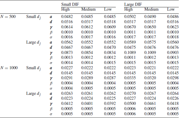
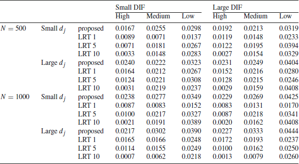
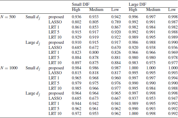


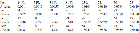

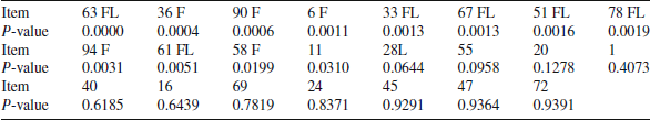

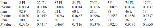


 Open access