


Introduction
People in more economically developed societies are increasingly disconnected from the natural world (Turner et al. Reference Turner, Nakamura and Dinetti2004, Soga & Gaston Reference Soga and Gaston2016), a trend often attributed to urbanization and reduced daily contact with nature (Miller Reference Miller2005, Maller et al. Reference Maller, Townsend, St Leger, Henderson-Wilson, Pryor and Prosser2009). In this context, green spaces in urban areas are central to mitigating this trend, as for many they represent their main way of interacting with the natural world on a daily basis (Natural England 2020). In the UK, provision of green space is highly variable across socioeconomic groups and geographical regions (Barbosa et al. Reference Barbosa, Tratalos, Armsworth, Davies, Fuller and Johnson2007). This is partly because a large proportion of green space in the UK is inaccessible, as it exists as private spaces such as domestic gardens (Mathieu et al. Reference Mathieu, Freeman and Aryal2007), and ownership of or access to private gardens varies with socioeconomic status and degree of urbanization (Harrison et al. Reference Harrison, Burgess and Millward1995, Coombes et al. Reference Coombes, Jones and Hillsdon2010, Dunton et al. Reference Dunton, Almanza, Jerrett, Wolch and Pentz2014). Across urbanized, economically developed societies, green space access is generally lower for children than for adults (Hand et al. Reference Hand, Freeman, Seddon, Recio, Stein and van Heezik2018, Veitch et al. Reference Veitch, Salmon and Ball2008). This is partly because of parental restrictions on freedom of movement (Hand et al. Reference Hand, Freeman, Seddon, Recio, Stein and van Heezik2018) grounded in concerns around safety (Timperio et al. Reference Timperio, Crawford, Telford and Salmon2004, Carver et al. Reference Carver, Timperio and Crawford2008) and partly because of urban barriers such as roads reducing access to local green spaces for children (Carver et al. Reference Carver, Timperio and Crawford2008, Villanueva et al. Reference Villanueva, Giles-Corti, Bulsara, McCormack, Timperio and Middleton2012).
However, urban green spaces can house a surprising amount of biodiversity. For example, one UK-based study found that urban areas contained significantly higher densities of blackbirds (Turdus merula), song thrushes (Turdus philomelos) and mistle thrushes (Turdus viscivorus) than the surrounding rural landscape (Mason Reference Mason2000), while another found that domestic gardens across five UK cities had higher flora richness than several natural habitats, including acidic grassland, acidic woodland, scrub and limestone grassland (Loram et al. Reference Loram, Thompson, Warren and Gaston2008).
Interaction with biodiversity is crucial for building a connection with nature and developing pro-environmental attitudes and behaviours later in life (Wells & Lekies Reference Wells and Lekies2006, The Wildlife Trusts & University of Derby 2019). For example, in one US-based study, participation in both ‘wild’ nature experiences (such as camping or hiking) and ‘domesticated’ nature experiences (such as harvesting or planting seeds) had a positive effect on likelihood of displaying environmental attitudes and behaviours in adulthood such as recycling or volunteering at a nature reserve (Wells & Lekies Reference Wells and Lekies2006). In the UK, those who took part in a month-long campaign to do something nature-related on a daily basis reported feeling more connected to nature and happier 2 months later (The Wildlife Trusts & University of Derby 2019). There have been calls to integrate research into the negative mental health effects of young people learning about environmental degradation with research on nature connection, so that the relationship between these ideas can be better understood (Chawla Reference Chawla2020). Overall, it is likely that improving access to experiences in the natural world from a young age is important for ensuring future engagement with conservation.
Evidence is divided as to whether well-being benefits scale with actual or perceived species richness. One study showed that mental well-being correlates with perceived richness but not with actual richness (Dallimer et al. Reference Dallimer, Irvine, Skinner, Davies, Rouquette and Maltby2012), while another found evidence that psychological benefits increase with habitat heterogeneity and actual plant richness (Fuller et al. Reference Fuller, Irvine, Devine-Wright, Warren and Gaston2007). Another found that an individual’s ability to perceive plant species richness accurately correlates positively with connection to nature and psychological well-being (Southon et al. Reference Southon, Jorgensen, Dunnett, Hoyle and Evans2018). People’s ability to accurately assess biodiversity may vary across different taxonomic groups, potentially mediated by the aesthetic cues people use to perceive species richness, such as flower colour and vegetation height (Southon et al. Reference Southon, Jorgensen, Dunnett, Hoyle and Evans2018). As a result, estimates of species richness for static components of a habitat such as plants can be more accurate than those for mobile components such as birds (Fuller et al. Reference Fuller, Irvine, Devine-Wright, Warren and Gaston2007, Dallimer et al. Reference Dallimer, Irvine, Skinner, Davies, Rouquette and Maltby2012).
It is likely that the health and well-being benefits of green space are mediated by aesthetic reactions to greenness and other landscape attributes, such as openness of view, colour diversity and vegetation height (Southon et al. Reference Southon, Jorgensen, Dunnett, Hoyle and Evans2018, Hoyle Reference Hoyle, Dempsey and Dobson2020), just as similar aesthetic cues, such as flower colour, play a key role in people’s perceptions of species diversity (Hoyle et al. Reference Hoyle, Norton, Dunnett, Richards, Russell and Warren2018). As such, several studies exploring the health and well-being benefits of green space have used settings that vary in visual greenness rather than measuring actual biodiversity differences (Ulrich Reference Ulrich, Altman and Wohlwill1983, Reference Ulrich1984, Reference Ulrich1986, Taylor et al. Reference Taylor, Kuo and Sullivan2001, Reference Taylor, Kuo and Sullivan2002, Hartig et al. Reference Hartig, Evans, Jamner, Davis and Gärling2003, Sullivan et al. Reference Sullivan, Kuo and DePooter2004, Tyrväinen et al. Reference Tyrväinen, Ojala, Korpela, Lanki, Tsunetsugu and Kagawa2014). Distinguishing between biodiversity and aesthetics, as well as avoiding confounding these two variables, will be important for improving our understanding of the relationship between these factors and their relative importance for well-being benefits.
Several studies have assessed the impacts of green school grounds on aspects of childhood well-being. Studies based in the Netherlands and the USA found that providing more green areas within school playgrounds led to a decrease in sedentary activity and an increase in physical activity (Bates et al. Reference Bates, Bohnert and Gerstein2018, van Dijk-Wesselius et al. Reference van Dijk-Wesselius, Maas, Hovinga, van Vugt and van den Berg2018), increases in positive social interactions and decreases in negative ones such as bullying or injuries (Bates et al. Reference Bates, Bohnert and Gerstein2018), positive effects on children’s appreciation of these spaces, attentional restoration and social well-being (van Dijk-Wesselius et al. Reference van Dijk-Wesselius, Maas, Hovinga, van Vugt and van den Berg2018) and a greater sense of competence and the formation of supportive relationships, providing protective resilience and improvements in responses to stress (Chawla et al. Reference Chawla, Keena, Pevec and Stanley2014). Children who spent more time in green playgrounds performed better on tests of self-regulation (Taylor & Butts-Wilmsmeyer Reference Taylor and Butts-Wilmsmeyer2020) and rated playgrounds with greater volumes of vegetation as more pleasant and conducive to the replenishment of mental resources (Bagot et al. Reference Bagot, Allen and Toukhsati2015). Benefits may also extend to educational attainment, with one study in Toronto finding that tree cover and species composition were positive predictors of student performance on standard assessments (Sivarajah et al. Reference Sivarajah, Smith and Thomas2018). More broadly, nature experiences during childhood have been shown to be key for: personal development, such as developing teamwork and problem-solving skills; environmental stewardship behaviours and attitudes, mediated by facilitating an emotional connection to nature; academic learning through improvements to self-discipline and stress responses; and the provision of rich sensory experiences that foster biodiversity understanding as well as broader learning opportunities (Beery & Jørgensen Reference Beery and Jørgensen2018, Kuo et al. Reference Kuo, Barnes and Jordan2019).
In this context, school grounds represent a potential priority area for biodiversity conservation because of their combined size and potential for joined-up management, their role in delivering well-being benefits and their central position in mediating the relationship between children and nature. Despite this, UK Government standards regulations for outdoor space in UK schools include no requirements for natural green spaces, instead focusing heavily on outdoor space for sports education and informal social play, with either hard (e.g., concrete or tarmac) or soft (e.g., synthetic turf, rubber or grass) coverings (Department for Education 2015). Guidelines mention ‘habitat areas’ (e.g., meadowland or gardens) for ‘supervised activities’, which ‘should generally be fenced to avoid unsupervised access’; however, provision of these habitat areas is not a requirement (Department for Education 2014).
A recent online survey of teachers at 1297 schools across England, Scotland and Wales gathered information on 12 different habitat types (including ponds, bird houses and planted borders) within school grounds and on whether or not the schools used their grounds to teach ecology (Harvey et al. Reference Harvey, Gange and Harvey2020). Despite all 12 habitat types being represented in their sample, there was wide variation in their frequency, with trees and planted borders being reported as present in c. 75% of schools, but wildflower meadows and bat boxes being reported as present in only c. 25% of schools. Only 58% of schools reported using their grounds to teach ecology, with a higher proportion of primary than secondary schools doing so (Harvey et al. Reference Harvey, Gange and Harvey2020). This suggests that while habitat types might be varied within schools, they are not being utilized fully for ecology-based education. Aside from this large-scale self-reported study, no studies have yet, to our knowledge, conducted in situ assessments of the biodiversity present at a fine scale in these spaces within the UK. It is vital to know what biodiversity is actually present within these spaces, as regular nature engagement with invertebrates can improve children’s awareness of invertebrate taxa from an initially vertebrate-biased perception of nature (Howlett & Turner Reference Howlett and Turner2023, Howlett et al. Reference Howlett, Lee, Jaffé, Lewis and Turner2023), and this improvement correlates with increased well-being and resilience in primary school-aged children (Montgomery et al. Reference Montgomery, Gange, Watling and Harvey2022).
In this study, we used a sample of 14 primary schools in England, including three school types (two state-funded (state and academy) and one non-state-funded (private)), in which we assessed levels of green space within and around each school and conducted in situ biodiversity surveys. We quantified greenness at three different levels: the area of green space in a 3-km buffer around each school including its grounds (buffer greenness); the area of green space within each school’s grounds (school greenness); and the amount of vegetation within each school’s grounds visible to children when outside in the grounds (visible vegetation). We quantified associated biodiversity within the schools by surveying trees, ground plants, ground invertebrates and birds. We assessed whether there were correlations between the three levels of greenness, whether the three levels of greenness varied between school types and whether abundance, richness and community composition of taxa varied with the three levels of greenness or school type.
Methods
Site selection
We sent out information about the study via the University Museum of Zoology, Cambridge’s mailing lists and social media accounts; 79 primary-school teachers at 57 different primary schools said they were happy to be contacted with further information. We arranged visits to as many of these schools as possible, limited by the schools’ capacities to host us, and collected biodiversity data from 14 schools in total (Table S1). Visits took place over the school holidays to avoid lesson disturbance, so the 14 schools that comprise our sample were self-selected from the initial pool of 57 schools. As we offered an educational biodiversity workshop in return for accommodating us, the schools’ motivations for helping us were educational rather than motivated by being particularly green or nature-friendly, helping to reduce potential bias from our small sample size. Schools were distributed across England, with the highest concentration occurring in the south-east (Fig. S2).
We visited both state-funded and non-state-funded schools, which we hereafter refer to as ‘school types’. We split state-funded schools into two categories – state and academy – reflecting different management practices. Although both categories are free to attend, academies are administratively free from local-authority control, whereas state schools are administered by their local authority with regards to admissions and day-to-day running. Non-state-funded schools, hereafter referred to as ‘private’, are paid for by parents and are not subject to local-authority control. We included this factor in our analyses because we were interested in understanding potential disparities in green space and biodiversity access between school types.
Data collection
Using QGIS (QGIS Development Team 2022), we calculated the area (m2) of outside space to which children had access for each school (i.e., the area of its grounds minus out-of-bounds areas such as car parks), as well as the area of a 3–km buffer around the school’s grounds. Using R version 4.1.3 (R Core Team 2022) and RStudio Build 461 (RStudio Team 2022), we then calculated the total number of pixels and the number of green pixels in each of these areas, which allowed us to calculate the area of green space (ha) in each of the school’s grounds (school greenness) and each of the 3–km buffers (buffer greenness). For each of the 14 schools, we also used Google Earth to overlay a 10 × 10 grid onto the outside area of each school to which children had access during the school day. We then used a random number generator to select 10 coordinates within this grid, which acted as our within-school sample locations. We assumed a priori that variability in habitats would not scale simply with school area, so we chose to adopt an approach that used an equal number of sample points per school. This also had the added benefit of allowing us to use school as a blocking variable in our multivariate generalized linear models (mGLMs) and as a random intercept effect in our generalized linear mixed models (GLMMs; see details below), thereby accounting for the potential random effect of individual schools on our results.
All school site visits were conducted in May–August 2019, September 2020 or August–September 2021 (Table S1). Visits were spread across three summers as we were limited by school availability and number of researchers and so could not fit all 14 visits into one summer.
Visible vegetation
At each of the 10 sample points per school, we took a photograph with an iPhone placed at 1 m above the ground facing each of the cardinal compass points, giving four images per sample point and 40 images per school. We then used an online image editor (MockoFUN 2022) to overlay a 10 × 10 grid onto each of the images and counted the number of squares in which any plant life was visible. Squares were counted as green even if there was only partial cover by plant life. Bare soil was not counted but fallen leaves were. We then took the proportion of squares in which plant life was present as a score of ‘visible vegetation’. The majority of the photographs taken were of an open view; however, to guard against our measure of visible vegetation being overly influenced by individual objects appearing close to the camera and masking vegetated views, we took the average of the four photographs at each point to give the proportion covered by plant life (‘visible vegetation’) at each sample point as a number between 0 and 1.
Trees
For all trees within school grounds, we identified each to morphospecies level and measured its diameter at breast height (DBH; cm). Morphospecies classification is a quick way of grouping organisms based on similar morphology for the purposes of later analysis. We chose DBH since this provides a good measure of tree maturity and is a correlate of canopy size, and so it is also relevant to children’s perceptions of greenness. For each school (n = 13), we calculated the number of trees (abundance), number of tree morphospecies (richness), mean DBH, maximum DBH and standard deviation in DBH. We were unable to collect these data for one of our 14 schools (Table S1) as maintenance staff estimated that there were >800 trees, and so, due to research team staff and resource constraints, we could not survey the whole site.
Ground plants
At each of the 10 sample points per school, we used a 0.5-m × 0.5-m quadrat (n = 110) to count the number of squares in which each morphospecies of plant (e.g., grass, moss, nettle), type of organic litter (e.g., bare soil, dead leaves, dead wood) or type of artificial surface (e.g., tarmac, AstroTurf) was present. All quadrats were taken in late July, August or early September.
Ground invertebrates
At each of the 10 points per school, we sampled ground invertebrates using a Vortis suction sampler (n = 100), sampling for 16 s at each of the four corners of the quadrat (Arnold Reference Arnold1994, Brook et al. Reference Brook, Woodcock, Sinka and Vanbergen2008). All samples were collected in August or early September and between 09h00 and 15h00. Samples were preserved in 70% alcohol before being sorted and identified using a stereomicroscope.
We identified most invertebrates to order level. Exceptions were annelids (phylum), Diplopoda, Collembola, Acari and Mollusca (class) and Formicidae (family). Hereafter, we collectively refer to all invertebrate groups as orders. Identifying to order level allowed all samples to be identified with the resources available and provided an overview of the ground invertebrate community present in each school. One sample was degraded, so we assigned the average of the other nine samples from this school for abundance, order richness and community composition for analyses.
Birds
At each of the 10 sample points per school, we conducted a bird point count (n = 110), during which all birds seen in the school grounds or flying directly overhead were counted and identified. All point counts were conducted in August or early September and between 09h00 and 17h00, as this is when children are most likely to see birds. All birds were identified to species level, apart from gulls, which we identified to family level (Laridae) as they generally flew too high overhead to be reliably identified to a finer taxonomic resolution. Hereafter, we collectively refer to all bird groups as species.
Due to the enforcement of COVID-19 lockdown restrictions from March 2020, it was not possible to arrange a second site visit to four of our 14 schools, so we are lacking biodiversity data in some categories (Table S1).
Data processing and statistical analyses
All statistical analyses were performed in R version 4.1.3 (R Core Team 2022) within RStudio Build 461 (RStudio Team 2022). We used tidyr (Wickham & Girlich Reference Wickham and Girlich2022), RColorBrewer (Neuwirth & Brewer Reference Neuwirth and Brewer2022), ggsignif (Ahlmann-Eltze & Patil Reference Ahlmann-Eltze and Patil2021), ggplot2 (Wickham Reference Wickham2016) and cowplot (Wilke Reference Wilke2020) for data wrangling, exploration and visualization. Exploration followed Zuur et al. (Reference Zuur, Ieno and Elphick2010). We conducted Spearman’s rank correlation tests and Kruskal–Wallis tests using stats (R Core Team 2022), and fitted GLMMs using glmmTMB (Brooks et al. Reference Brooks, Kristensen, van Benthem, Magnusson, Berg and Nielsen2017) and mGLMs using mvabund (Wang et al. Reference Wang, Naumann, Eddelbuettel, Wilshire, Warton and Byrnes2022).
We used Spearman’s rank-order coefficient to test for correlations between all three pairs of levels of greenness (buffer greenness and school greenness; buffer greenness and visible vegetation; and school greenness and visible vegetation) and for correlations between each of tree abundance, morphospecies richness, mean DBH, maximum DBH and standard deviation in DBH and the three levels of greenness. Where notable outliers were present, we re-ran correlation tests without outliers to check the robustness of our results. Visible vegetation was averaged across all 40 images for each school to give a single score per school that ranged between 0 and 1. We used the same method to test for correlations between school area and school greenness and between school area and visible vegetation, as it is possible that the land area of a school, regardless of greenness, plays a key role in species diversity.
We used Kruskal–Wallis tests to test for differences between school types in each of the three levels of greenness and in school area and on each of the tree metrics, followed by Dunn’s tests with Bonferroni correction where school type was significant (p < 0.05). Visible vegetation was averaged across the four images taken at each sample point.
We used GLMMs to assess factors affecting ground plant morphospecies richness, ground invertebrate abundance and order richness and bird abundance and species richness. We fitted models to negative binomial distributions, including buffer greenness, school greenness, visible vegetation and school type as fixed effects and school as a random intercept effect to account for multiple measures at each school. GLMMs for ground invertebrate order richness and bird species richness were fitted to Poisson distributions due to issues with model fit with negative binomial distributions. Ground cover data for organic litter (e.g., bare soil, dead leaves, dead wood) and artificial surfaces (e.g., tarmac, AstroTurf) were excluded from ground plant morphospecies richness analyses.
We validated GLMMs by plotting quantile residuals against predicted values and covariate school type to verify that no patterns were present. To ensure our GLMMs fitted the observed data, we ran simulation-based dispersion tests using DHARMa (Hartig Reference Hartig2022) to compare the variance of the observed residuals against the variance of the simulated residuals, with variances scaled to the mean simulated variance, and we checked that our model was within the range of our simulations (Zuur & Ieno Reference Zuur and Ieno2016). Our simulations indicated that there were no issues with model fit. We determined the significance of fixed effects to each model by comparing fitted models with null models using likelihood ratio tests (LRTs). If mixed models suggested a moderately significant effect (0.03 < p < 0.07), we re-calculated p-values based on parametric bootstrapping using DHARMa (Bates et al. Reference Bates, Mächler, Bolker and Walker2015, Hartig Reference Hartig2022). If school type was significant, we used multcomp (Hothorn et al. Reference Hothorn, Bretz and Westfall2008) to conduct post-hoc analyses (Tukey all-pair comparisons, adjusting p-values using Bonferroni correction) to identify school types between which significant differences occurred.
We used mGLMs to analyse community composition of all taxa (Warton et al. Reference Warton, Wright and Wang2012, Warton & Hui Reference Warton and Hui2017), fitting models to negative binomial distributions, including buffer greenness, school greenness, visible vegetation and school type as fixed effects and school as a blocking variable to account for non-independence of samples within each school. Ground cover data for organic litter (e.g., bare soil, dead leaves, dead wood) and artificial surfaces (e.g., tarmac, AstroTurf) were included in ground cover community composition analyses.
We validated mGLMs by plotting Dunn–Smyth residuals against fitted values and covariate school type to verify that no patterns were present (Wang et al. Reference Wang, Naumann, Wright and Warton2012, Reference Wang, Naumann, Eddelbuettel, Wilshire, Warton and Byrnes2022). We determined the significance of fixed effects using LRTs and by bootstrapping probability integral transform residuals using 10 000 resampling iterations (Warton et al. Reference Warton, Thibaut and Wang2017). If school type was significant (p < 0.05), we ran univariate analyses on individual taxa. We adjusted univariate p-values to correct for multiple testing using a step-down resampling algorithm (Wang et al. Reference Wang, Naumann, Wright and Warton2012), but otherwise our statistical approach remained unchanged from the multivariate parent models.
For both GLMMs and mGLMs, visible greenness was averaged across the four images taken at each sample point.
Results
Across the 14 schools, we found 36 tree morphospecies, 47 types of ground cover (including 40 plant morphospecies, four types of organic litter and three types of artificial surface), 17 invertebrate orders and 23 bird species. The most abundant tree morphospecies were birch, maple and lime (Fig. S3a). The most common types of ground cover were grass, tarmac and bare soil (Fig. S3b). The most abundant plant morphospecies were grass, white clover (Trifolium repens) and greater plantain (Plantago major; Fig. S3b). The most abundant ground invertebrate orders were Collembola, Acari and Hemiptera (Fig. S3c). The most abundant bird species were wood pigeons (Columba palumbus), crows (Corvus corone) and house sparrows (Passer domesticus; Fig. S3d).
Correlations between levels of greenness
Visible vegetation correlated with school greenness (S = 46, p = 0.006, ρ = 0.7909; Fig. 1a), such that schools with larger areas of green space in their grounds had higher amounts of visible vegetation, a trend that was particularly driven by a single private school with an especially large area of green space (Fig. 1a) but which remained significant after re-running the analysis without this school (S = 44, p = 0.02117, ρ = 0.7333), although with a different gradient. Buffer greenness did not correlate with school greenness (S = 350, p = 0.4265, ρ = 0.2308; Fig. 1b) or visible vegetation (S = 132, p = 0.225, ρ = 0.4; Fig. 1c). School area had highly significant positive correlations with school greenness (S = 12, p < 0.00001, ρ = 0.9736) and visible vegetation (S = 74, p = 0.03085, ρ = 0.6636).
Scatter plots of relationships between levels of greenness. Points are coloured by school type. (a) School greenness (ha) against visible vegetation, as a mean of 40 photographs per school (n = 11; blue line shows a simple linear model, with the grey area indicating a 95% confidence interval). (b) Buffer greenness (ha) against school greenness (ha; n = 14). (c) Buffer greenness (ha) against visible vegetation, as an average of 40 photographs per school (n = 11).

Buffer greenness
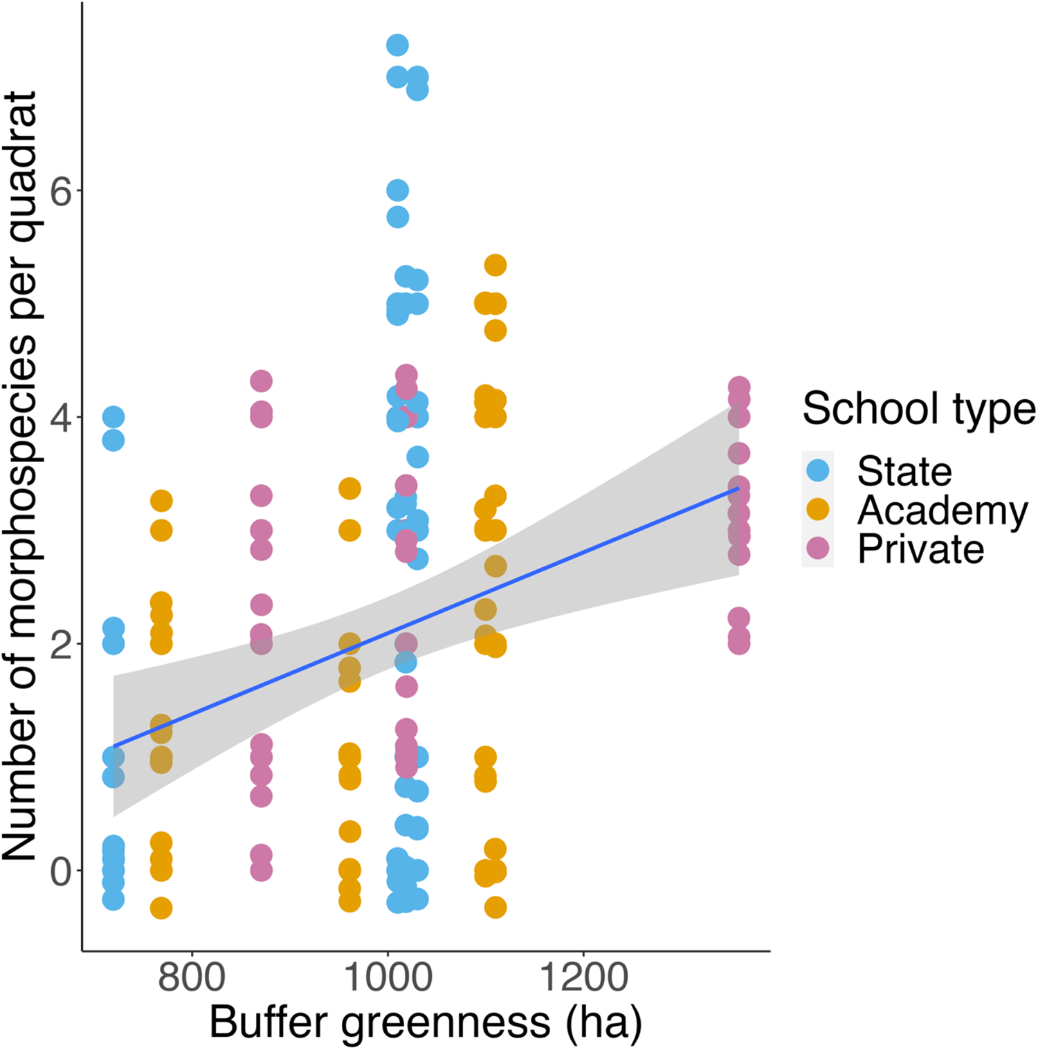
Schools with greater buffer greenness had higher quadrat plant morphospecies richness (LRT = 6.9104, p = 0.00857; Fig. 2), but there were no effects on any other biodiversity measure.
Scatter plot showing buffer greenness (ha) against quadrat plant morphospecies richness (n = 110). Points are coloured by school type. Blue line shows a simple linear model, with the grey area indicating a 95% confidence interval.
School greenness
Schools with higher school greenness had greater tree abundance (S = 114, p = 0.01201, ρ = 0.6868; Fig. 3a) and morphospecies richness (S = 106.29, p = 0.006772, ρ = 0.7080; Fig. 3b), trends that remained significant after re-running our analyses without the outlier school included (tree abundance: S = 114, p = 0.04281, ρ = 0.6014; tree morphospecies richness: S = 106.37, p = 0.02875, ρ = 0.6281). There was also a significant effect of school greenness on tree community composition (LRT = 144.4282, p = 0.03040), although univariate analyses indicated that this was not driven by any morphospecies in particular. There were no effects on any other biodiversity measure.
Relationships between school greenness and (a) tree abundance per school (n = 13) and (b) tree morphospecies richness per school (n = 13). Points are coloured by school type. Blue lines show simple linear models, with the grey areas indicating 95% confidence intervals.

Visible vegetation
Schools with higher visible vegetation had greater tree abundance (S = 40, p = 0.01592, ρ = 0.7576; Fig. 4a) and morphospecies richness (S = 52, p = 0.03509, ρ = 0.6848; Fig. 4b), greater maximum tree DBH (S = 48, p = 0.02751, ρ = 0.7091; Fig. 4c), greater quadrat plant morphospecies richness (LRT = 22.3433, p < 0.0001; Fig. 4d) and greater invertebrate abundance (LRT = 68.494, p < 0.0001 Fig. 4e) and order richness (LRT = 76.332, p < 0.0001; Fig. 4f). There was a significant effect of visible vegetation on quadrat community composition (LRT = 207.5057, p < 0.0001), with univariate analyses indicating that this effect was driven by differences in coverage by tarmac (p = 0.04590), dead leaves (p < 0.0001) and grass (p = 0.0009999). There was also a significant effect of visible vegetation on ground invertebrate community composition (LRT = 261.8301, p < 0.0001), with univariate analyses indicating that this effect was driven by differences in abundance of Formicidae (p = 0.0066), Coleoptera (p = 0.0002), Hemiptera (p < 0.0001), Diptera (p = 0.0006), Hymenoptera (p < 0.0001), Araneae (p < 0.0001), Collembola (p < 0.0001), Thysanoptera (p = 0.0039), Acari (p < 0.0001), Isopoda (p = 0.0227) and Psocoptera (p = 0.0227). There was no effect of visible vegetation on any other biodiversity measure.
Effects of visible vegetation. Points are coloured by school type. Blue lines show simple linear models, with the grey areas indicating 95% confidence intervals. Scatter plots showing visible vegetation against: (a) tree abundance per school (n = 13); (b) tree morphospecies richness per school (n = 13); (c) maximum tree diameter at breast height (DBH; cm) per school (n = 13); (d) plant morphospecies richness per quadrat (n = 110); (e) vertebrate abundance per sample (n = 100); and (f) invertebrate order richness per sample (n = 100).

School type
Visible vegetation differed significantly between school types (χ2 = 33.648, df = 2, p < 0.0001; Fig. 5a), with post-hoc tests showing that visible vegetation was higher in private schools than in the other two school types, which did not differ from each other (Table S4). However, there was no difference between school types in buffer greenness (χ2 = 0.1114, df = 2, p = 0.9458), school greenness (χ2 = 3.2429, df = 2, p = 0.1976) or school area (χ2 = 2.6914, df = 2, p = 0.2604).
Boxplots showing differences between school types in (a) visible vegetation per image (n = 440) and (b) tree diameter at breast height (DBH; cm; n = 945). Brackets labelled with adjusted p-values show significant differences between pairs of school types following post-hoc analyses (Table S4). Black lines indicate median values. Coloured boxes show interquartile ranges (IQRs). Whiskers extend to the largest and smallest values no further than 1.5 × IQR. SD = standard deviation.

Maximum tree DBH differed marginally between school types (χ2 = 6.4879, df = 2, p = 0.03901; Fig. 5b), although post-hoc analyses indicated that there were no pairwise differences (Table S4). Standard deviation in tree DBH differed between school types (χ2 = 6.5423, df = 2, p = 0.03796; Fig. 5b), with post-hoc analyses indicating that the standard deviation in DBH in private schools was higher than in state schools, but there were no differences between the other two pairs of school types (Table S4). There was a significant effect of school type on ground invertebrate community composition (LRT = 151.2539, p = 0.007599), with univariate analyses indicating that this effect was driven by greater numbers of Hymenoptera in academies than in state schools (p = 0.04260). There was no effect of school type on any other biodiversity measure.
Discussion
This is the first study to systematically record the environmental characteristics and biodiversity of multiple school grounds in the UK. Our findings suggest that, while the amount of green space both surrounding and within schools is highly variable, these spaces house a range of different taxa. As active engagement with nature and exposure to smaller taxa such as invertebrates are important for shaping perceptions of nature (Montgomery et al. Reference Montgomery, Gange, Watling and Harvey2022), these spaces are therefore likely to be important for the development of nature connection and ecological knowledge in children (Wells & Lekies Reference Wells and Lekies2006, The Wildlife Trusts & University of Derby 2019). This mirrors research on other types of urban green space, which has recorded relatively high levels of species richness in relatively small urban spaces, such as domestic gardens (Gaston Reference Gaston2007, Loram et al. Reference Loram, Thompson, Warren and Gaston2008, Ives et al. Reference Ives, Lentini, Threlfall, Ikin, Shanahan and Garrard2016), but inequality in access across demographic groups and geographical regions (Barbosa et al. Reference Barbosa, Tratalos, Armsworth, Davies, Fuller and Johnson2007, Mathieu et al. Reference Mathieu, Freeman and Aryal2007, Dunton et al. Reference Dunton, Almanza, Jerrett, Wolch and Pentz2014). Since our study is based on a relatively low number of self-selecting schools, these results should be treated with caution. However, offer of an educational reward for participation means that schools were unlikely to be systematically biased, and significant results from even our small sample size indicate that results are robust.
The area of green space in a 3–km buffer around a school’s grounds (buffer greenness) did not correlate with the area of green space within a school’s grounds (school greenness), nor with the amount of vegetation visible in images taken in the grounds (visible vegetation). However, schools with a larger area of green space in their grounds (school greenness) had higher levels of vegetation within their grounds (visible vegetation). This suggests that the amount of green space children have access to at school is not reflective of the amount of green space in the local environment, but that schools with larger areas of outside space with natural cover are able to support greater amounts of vegetation within their grounds in the form of more shrubs, trees and other visible plant life. This finding highlights the importance of the provision of green space in school grounds beyond that used for sports or exercise for increasing children’s exposure to nature. Given that we also found school area to correlate positively with school greenness and visible vegetation, it is possible that our biodiversity results could also be related to the land area of schools, in line with species–area relationships. This could be most influential on trees, as they are constrained entirely by green area, while other taxa, such as birds, can move through the landscape and use other available habitats in the local area.
Larger areas of green space in the buffer correlated with higher morphospecies richness of ground plants, but buffer greenness had no effect on any measure of tree, invertebrate or bird biodiversity, nor on community composition of ground cover. This indicates that greener local environments may be important for maintaining the diversity of ground plants but have limited impacts on larger taxa or those of higher trophic levels. This presumably reflects the potential for plant species within urban green spaces to colonize via seed rain from surrounding areas (Mathey et al. Reference Mathey, Rößler, Banse, Lehmann and Bräuer2015, Jim et al. Reference Jim, Konijnendijk and Chen2018), leading to higher diversity where such areas are more extensive.
Schools with larger areas of green space in their grounds had more trees and greater tree morphospecies richness. The area of green space in a school’s grounds also affected community composition of trees, but it had no effect on any measure of ground plant, invertebrate or bird biodiversity. This suggests that larger amounts of green space in school grounds result in greater tree diversity, but that greenness at this scale does not translate into greater diversity of other taxa. This is most likely related to what trees school staff decide to plant on the basis of the space they have available, indicating that schools with more green space at their disposal are able to take advantage of this through increasing tree diversity. This is encouraging given that previous research has demonstrated links between tree cover specifically, as opposed to other types of green cover, and better performance by pupils on standardized school tests of maths and reading skills (Kuo et al. Reference Kuo, Browning, Sachdeva, Lee and Westphal2018, Sivarajah et al. Reference Sivarajah, Smith and Thomas2018). Further research has also demonstrated the importance of tree planting within 250 m of school buildings to supporting academic performance (Kuo et al. Reference Kuo, Klein and Zaplatosch2021), as well as the importance of tree shade in mitigating the impacts of heat on children’s play areas (Lanza et al. Reference Lanza, Alcazar, Hoelscher and Kohl2021). However, the majority of school outside spaces are currently dominated by grass and hard artificial surfaces, such as tarmac, with trees accounting for the smallest proportion of school land use (Schulman & Peters Reference Schulman and Peters2008). Our finding that schools with a greater area of green space at their disposal also supported greater vegetation, such as trees and shrubs, therefore provides a powerful argument for increasing the amount of outside green space available to UK schools.
Schools with higher visible vegetation in their grounds had more trees, greater tree morphospecies richness, higher maximum tree DBH, higher morphospecies richness of ground plants and higher abundance of ground invertebrates. The amount of vegetation also affected the community composition of ground cover and ground invertebrates, but it had no effect on the community composition of trees, invertebrate order richness or any measure of bird biodiversity. This suggests that greenness at this finest scale affects the greatest number of taxa, and this is therefore the most important scale to prioritize for management strategies that seek to maximize school biodiversity. This is also the scale at which children are most likely to experience greenness, since photographs were captured at a height of 1 m above the ground, so maximizing biodiversity at this scale is also likely to have the greatest impact on children. Increasing the naturalness of children’s views while at school, both while outside and from within the classroom through windows, is likely to be important in helping children mitigate stress levels and improve their attention and pro-social behaviour (Li & Sullivan Reference Li and Sullivan2016, Amoly et al. Reference Amoly, Dadvand, Forns, López-Vicente, Basagaña and Julvez2014).
Encouragingly, while little can be done to increase the amount of green space surrounding a school or the amount of outside green space within a school’s existing grounds, maximizing the amount of vegetation within a school through the maintenance and planting of trees, shrubs and other plants within existing areas represents the easiest and most effective way to maximize biodiversity within school grounds in the UK. In addition to contributing to biodiversity conservation, this could be an effective way to increase the engagement of children with nature and improve ecological awareness. This is particularly the case since small taxa, such as ground invertebrates, represent a more practical pathway through which children can interact with and learn about the natural world than larger taxa (Montgomery et al. Reference Montgomery, Gange, Watling and Harvey2022), such as mammals, which are typically more elusive and less abundant. Increasing the amount of vegetation within school grounds through active planting also supports activities such as gardening, which have been linked both with improved science knowledge and with improved engagement with science learning (Wells et al. Reference Wells, Myers, Todd, Barale, Gaolach and Ferenz2015, Williams et al. Reference Williams, Brule, Kelley and Skinner2018).
Private schools had higher levels of visible vegetation than both types of state-funded schools, which did not differ from each other. There were no differences between school types in the area of green space in the buffer or within school grounds, or in the overall school area. This suggests that the amount of vegetation within school grounds is reflective of management practices rather than surrounding green space, and consequently that children who attend fee-paying schools in England may be exposed to more vegetation than those who attend state-funded schools. This is probably because the satellite imagery used here to measure buffer greenness and school greenness captures greenness as a 2D area (e.g., size of a grass-covered playing field), but the on-site photographs, by virtue of being taken perpendicular to the ground to capture children’s actual perception, are capturing a 3D measure of vegetation (e.g., whether a playing field is bordered by trees and shrubs versus a wooden fence). Therefore, our results suggest that, while all schools (private schools included) broadly have a playing field of similar size, private schools have more actual 3D vegetation in their grounds. Previous research has shown that higher amounts of tree cover and tree species diversity can lead to improved educational performance in primary school pupils (Wu et al. Reference Wu, McNeely, Cedeño-Laurent, Pan, Adamkiewicz and Dominici2014, Sivarajah et al. Reference Sivarajah, Smith and Thomas2018) and that greener school grounds are associated with improved cognitive, emotional and behavioural performance (Wells Reference Wells2000, Bijnens et al. Reference Bijnens, Derom, Thiery, Weyers and Nawrot2020, Taylor & Butts-Wilmsmeyer Reference Taylor and Butts-Wilmsmeyer2020), so our findings have implications for educational outcomes in state-funded versus privately funded schools in the UK. As a caveat, we have not been able to take into account historical data on previous land use for schools or their local surroundings as these data were not available, so it is possible that these factors could have influenced our biodiversity results.
Standard deviation and maximum tree DBH per school differed between school types, with private schools having greater standard deviation in tree DBH than state schools but with no pairwise differences in maximum DBH. School type also affected the community composition of ground invertebrates, with academies having greater numbers of Hymenoptera than state schools. It is likely that the greater range in tree DBH in private schools than in both kinds of state schools represents greater long-term consistency in ground management, giving trees more time to mature and resulting in more mature trees in private schools in addition to newly planted ones. This is therefore likely to reflect differences in management decisions or school age. State-funded schools have declining rates of retention for those in leadership roles (Lynch et al. Reference Lynch, Mills, Theobald and Worth2017, Department for Education 2018), and there is currently high pressure on the state school system in England, with rising demand for places and increasing class sizes (Morse Reference Morse2013), so state schools may have been forced to prioritize infrastructure developments over maintaining mature trees.
Conclusions and recommendations
Collectively, our study indicates that UK primary school grounds can house a wide range of taxa relative to their small size, and that these are broadly consistent across private- and state-funded systems, making school grounds a priority for biodiversity conservation and engaging younger generations with nature. This implies that a similar conservation strategy, which will benefit biodiversity and provide educational opportunities and well-being improvements, can be applied across education systems.
However, we also found that levels of greenness likely to be seen by students, as well as some aspects of biodiversity, were higher in private- than state-funded schools, indicating that students at state-funded schools may have less exposure to green space and associated nature. We suggest that prioritizing increasing the amount of vegetation in school grounds through the maintenance and planting of trees, shrubs and other plants and the greening of hard infrastructure through containers or green roofs represents both the most practical and most effective method to increase biodiversity within schools.
Since visible vegetation was correlated with high diversity in several taxa, this suggests that our in situ method of photographing vegetation was a reasonable indicator of school biodiversity. As such, a similar measure, based on citizen-science photographs of school vegetation, could be used as a surrogate for more in-depth biodiversity surveys to build a national picture of school biodiversity through remote methods, allowing the identification of schools with especially low biodiversity that could benefit from targeted additional funding to enhance their green spaces. Given our modest sample size of 14 schools focused largely on the south-east of England, this represents a promising remote method through which to quantify biodiversity across a larger national network of schools, whilst also providing the opportunity for school students themselves to get involved in citizen science. More generally, the trends we identified here in our small sample merit further investigation via more detailed in situ biodiversity surveys across a wider range of schools within the UK.
We recommend that greater requirements for outside learning and ecology-specific topics are integrated into national curricula to take advantage of the existing green space to which schools have access and to maximize the benefits of this important resource, which has been underused (Harvey et al. Reference Harvey, Gange and Harvey2020).
Supplementary material
For supplementary material accompanying this paper visit https://doi.org/10.1017/S0376892923000255.
Acknowledgements
We thank the Public Engagement team at the University Museum of Zoology, Cambridge, and all participating schools, teachers and students for their support with this project.
Financial support
Kate Howlett is funded by the Natural Environment Research Council (grant number NE/L002507/1).
Competing interests
The authors declare none.
Ethical standards
None.


 Open access