


Introduction
Glacier and ice-sheet models are valuable tools to assess their future evolution and the resulting sea-level rise under climate warming (Pattyn, Reference Pattyn2018). In the past two decades, tremendous efforts have been made by the glaciological community to develop models to account for the most relevant underlying physical processes such as ice flow, thermodynamics, subglacial hydrology and their coupling with the atmosphere (e.g. climate-driven surface mass balance), the lithosphere, and the ocean (e.g. iceberg calving or subaquatic melt). However, the added complexity of these models comes with increasing computational cost, which cannot be offset entirely by recent advances in scalable numerical methods and increasing computing power.
Since the 1950s, ice is commonly treated as a viscous, non-Newtonian fluid (Glen, Reference Glen1953) best described by the Stokes equations, which are computationally expensive to solve. Although numerical simulations of real small glaciers have been possible since the late 1990s (e.g. Gudmundsson, Reference Gudmundsson1999), the simulation of large icefields and ice sheets at high spatial resolution and/or over multi-millennial time scales remains challenging with today's available computational resources, with a few exceptions: Seddik and others (Reference Seddik, Greve, Zwinger, Gillet-Chaulet and Gagliardini2012) performed a 100-year simulation of the entire Greenland Ice Sheet while Cohen and others (Reference Cohen, Gillet-Chaulet, Haeberli, Machguth and Fischer2018) modelled a few millennia of the former Rhone Glacier at the Last Glacial Maximum with Elmer/Ice (Gagliardini and others, Reference Gagliardini2013). As a consequence, most models frequently solve computationally less expensive approximations to the Stokes equations.
The Shallow Ice Approximation (SIA; Hutter, Reference Hutter1983), a zeroth-order approximation to the Stokes equations, remains a reference model for many applications (e.g. Maussion and others, Reference Maussion2019; Višnjević and others, Reference Višnjević, Herman and Prasicek2020), despite strongly-simplifying mechanical assumptions and applicability limited to areas where ice flow is dominated by vertical shearing (Greve and Blatter, Reference Greve and Blatter2009). As a compromise between mechanical accuracy and computational costs, a family of models of intermediate complexity has emerged such as the hybrid SIA + SSA (Shallow Shelf Approximation) (Bueler and Brown, Reference Bueler and Brown2009) implemented in the Parallel Ice Sheet Model (PISM) (Khroulev and the PISM Authors, Reference Khroulev2020). This class of approximations reduces the stress balance to at most 2-D equations, thus facilitating simulations over time scales of glacial cycles (Seguinot and others, Reference Seguinot2018). With the exception of sub-glacial hydrology models (Werder and others, Reference Werder, Hewitt, Schoof and Flowers2013), the costs associated with the other glacier-related model components (e.g.mass balance, ice energy, lithospheric displacement, calving) remain computationally low. Well-established and state-of-the-art simulation tools such as PISM or Elmer/Ice already use efficient and scalable numerical solvers, thus limiting the potential for further improvements in computational efficiency. Yet computational efficiency in high-order ice flow modelling is crucial to (i) explore a large variety of model parameters, (ii) model long time scales in paleo applications, (iii) refine the spatial resolution when dealing with complex topography, and (iv) to reduce model biases where SIA-like models are used today due to computational constraints.
In recent years, Graphics Processing Units (GPU), which feature more but slower cores compared to Central Processing Units (CPU), have gained interest in ice flow modelling to overcome the aforementioned limitations, and to obtain significant speed-ups (Räss and others, Reference Räss, Licul, Herman, Podladchikov and Suckale2020). The key for using GPUs efficiently is to implement numerical schemes that can be divided into several thousand parallel tasks; a challenge regarding the viscous behaviour of ice, and the underlying diffusion equations that describe its motion. To our knowledge, two approaches have been attempted to achieve this high level of parallelization. The first consisted of solving SIA (Višnjević and others, Reference Višnjević, Herman and Prasicek2020) or Second Order SIA (Brædstrup and others, Reference Brædstrup, Damsgaard and Egholm2014), explicitly in time, while the second consisted of solving the Stokes equations using finite differences to take advantage of numerical stencil-based techniques (Räss and others, Reference Räss, Licul, Herman, Podladchikov and Suckale2020). The first approach permitted a large ensemble or long time scales simulations with applications to invert climatic parameters from observed glacial extents at the last glacial maximum (Višnjević and others, Reference Višnjević, Herman and Prasicek2020) and to model glacial erosion and landscape evolution over glacial cycle time scales (Egholm and others, Reference Egholm2017). The necessity of coding in a dedicated programming language (e.g. CUDA) has probably hindered the use of GPUs. However, the emergence of user-friendly Python libraries such as TensorFlow and PyTorch, which allow running relatively simple code on GPUs, will certainly contribute to popularize it in the coming years.
Compared to physic-based numerical models (referred here as instructor models), statistical emulators (or surrogate models), which mimic the behaviour of the simulator as closely as possible, are computationally cheap to evaluate. Surrogate models are solely constructed from intelligently chosen input-output data of the instructor model without any knowledge of its inner working. The arrival of machine learning has led to the development of deep learning-based surrogate models (Reichstein and others, Reference Reichstein2019) to accelerate computational fluid dynamics (CFD) codes (e.g. Ladicky and others, Reference Ladický, Jeong, Solenthaler, Pollefeys and Gross2015; Tompson and others, Reference Tompson, Schlachter, Sprechmann and Perlin2016; Kim and others, Reference Kim, Azevedo, Thuerey, Kim, Gross and Solenthaler2019; Obiols-Sales and others, Reference Obiols-Sales, Vishnu, Malaya and Chandramowlishwaran2020). The main idea is to take advantage of the large amount of modelling results (data) that a CFD solver can produce to train a neural network emulator delivering high fidelity solutions at much lower computational cost. The fidelity of the emulated solution, relative to the instructor model, is directly dictated by the emulator complexity and the quality of the training dataset, which must be representative of all dynamical states. This approach can therefore be seen as a way to compress a large number of model realizations (Kim and others, Reference Kim, Azevedo, Thuerey, Kim, Gross and Solenthaler2019), and to take benefit of this information for new model runs that are fairly close to the runs already performed in generating the training dataset. With the exception of Brinkerhoff and others (Reference Brinkerhoff, Aschwanden and Fahnestock2021), this idea has never been exploited in ice flow modelling. Yet – from a CFD point of view – the most accurate and most expensive ice flow model, the Stokes model, shows no major difficulties for its numerical solving: it is a purely diffusive (although non-linear) non-advective, time-independent problem, and its solution solely depends on the geometry, and given fields such as the ice hardness or the basal sliding coefficient. Furthermore, the same solver often recomputes states which are close to those which were computed before for parameter studies (Aschwanden and others, Reference Aschwanden2019) or multi-glacial cycle applications (Sutter and others, Reference Sutter2019). In such cases, the strategy described above can be very beneficial to use previously computed ice flow modelled states and save this information to emulate a cheap model trained by deep learning. This paper intends to explore the potential of constructing ice flow model emulators.
In the machine learning paradigm, Artificial Neural Networks (ANNs) have been increasingly used in recent years to deal with various kinds of problems such as image classification (Simonyan and Zisserman, Reference Simonyan and Zisserman2015), segmentation (Ronneberger and others, Reference Ronneberger, Fischer and Brox2015) and domain transfer (Isola and others, Reference Isola, Zhu, Zhou and Efros2017), whenever a large-scale training dataset is available (LeCun and others, Reference LeCun, Bengio and Hinton2015). Classical examples of classifiers are email filtering to identify spam (Dada and others, Reference Dada2019), handwriting recognition (Cireşan and others, Reference Cireşan, Meier, Gambardella and Schmidhuber2010)or image segmentation for biomedical applications (Yang and others, Reference Yang, Zhang, Chen, Zhang and Chen2017). In the case of image analysis, a breakthrough occurred in the early 2010s (LeCun and others, Reference LeCun, Bengio and Hinton2015) thanks to successful Convolutional Neural Networks (CNN) that are today widely used in image recognition or classification. CNNs are especially good at recognizing image features or spatial patterns due to convolution operations, and their optimization is computationally tractable owing to a strategy of shared weights to reduce the number of tuning parameters.
In glaciology, ANNs have been used for estimating bed topography (Clarke and others, Reference Clarke, Berthier, Schoof and Jarosch2009; Leong and Horgan, Reference Leong and Horgan2020; Monnier and Zhu, Reference Monnier and Zhu2021), to infer basal conditions at the bedrock (Brinkerhoff and others, Reference Brinkerhoff, Aschwanden and Fahnestock2021; Riel and others, Reference Riel, Minchew and Bischoff2021), to model mass balance (Bolibar and others, Reference Bolibar2020) or to identify the calving fronts of tidewater glaciers from satellite images (Baumhoer and others, Reference Baumhoer, Dietz, Kneisel and Kuenzer2019; Mohajerani and others, Reference Mohajerani, Wood, Velicogna and Rignot2019; Zhang and others, Reference Zhang, Liu and Huang2019; Cheng and others, Reference Cheng2021). Note that the last three studies all rely on semantic image segmentation using CNN. Recently, Brinkerhoff and others (Reference Brinkerhoff, Aschwanden and Fahnestock2021) used a neural network to emulate an expensive coupled ice flow/subglacial hydrology model, and infer the optimal parameters that best reproduce the observed surface velocities using a Bayesian approach.
In this paper, we apply deep learning to ice flow modelling. Our approach consists of setting up a CNN that predicts ice flow from given topographic variables and basal sliding parametrization in a generic manner. By contrast, Brinkerhoff and others (Reference Brinkerhoff, Aschwanden and Fahnestock2021) emulated a coupled ice flow-hydrology model for a specific glacier from a small-size ensemble of relevant parameters. Our neural network emulator is trained from a large dataset, which is generated from ice flow simulations obtained from two state-of-the-art models – the PISM (Khroulev and the PISM Authors, Reference Khroulev2020) and CfsFlow (Jouvet and others, Reference Jouvet, Picasso, Rappaz and Blatter2008, Reference Jouvet, Huss, Blatter, Picasso and Rappaz2009) – equipped with two different mechanics (hybrid SIA + SSA and Stokes) and at two different spatial resolutions (2 km and 100 m). We integrate mass balance and mass conservation with our ice flow emulator to obtain a time evolution model, the ‘Instructed Glacier Model’ (IGM) written in Python, which permits highly efficient, and mechanically state-of-the-art ice flow simulations.
In the following, we first describe the IGM model with its neural network-based emulator and the generation of the training dataset. Then, we present our results in terms of fidelity and computational performance of the emulated ice flow model with respect to the instructor model, and of embedding the ice flow emulator into a time evolution model. Last, we compare and discuss the IGM results with state-of-the-art ice flow model results.
Methods
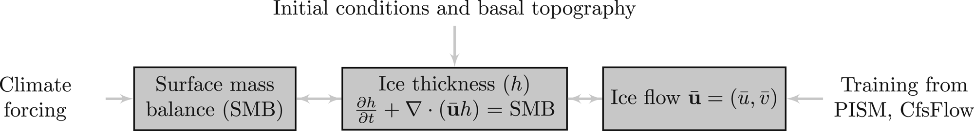
IGM couples the submodels of surface mass balance, mass conservation and ice dynamics as depicted in Figure 1. Specifically, IGM models the ice flow by a CNN emulator, which is trained by PISM and CfsFlow realizations.
Interactions between the model components and the input data of IGM.
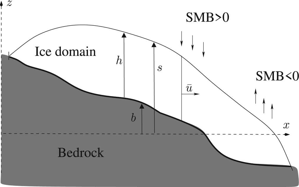
From now on, we denote b(x, y), h(x, y, t) and s(x, y, t) = b(x, y) + h(x, y, t) bedrock elevation (assumed to be fixed in time), ice thicknessand ice surface elevation, respectively (Fig. 2). We call $\bar {\bf u} = ( \bar {u},\; \bar {v})$ the vertically-averaged horizontal ice velocity field, and SMB the Surface Mass Balance function, which consists of yearly-average accumulation (when positive) or ablation (when negative). Given $\bar {\bf u}$
 and the SMB function, and ignoring basal melt, the evolution in ice thickness h is determined by the mass conservation equation:

which states the balance between the change in ice thickness ∂h/∂t, the dynamical thinning/thickening $\nabla \cdot ( \bar {\bf u} h)$ due to the ice flux $\bar { \bf u} h$
 , and the adding/removal of ice on the top surface by the SMB (Fig. 2). Here $\nabla \cdot$
 denotes the divergence operator with respect to horizontal variables (x, y).
Cross-section of a glacier with notations.
We assume the horizontal model domain to be a rectangle subdivided by a regular 2-D grid with uniform spacing Δx in x and y – the variables h, s, b, $\bar {u}$ , $\bar {v}$
 , SMB being defined at the centre of each cell. Let t 0 be the initial time, {t k}k=0,1,… be a discretization of time with variable steps Δt k+1 = t k+1 − t k. We denote by h k an approximation of h at time t = t k, and similarly for all other variables. Given an initial ice thickness h 0, IGM updates the ice flow $( \bar {u}^{k},\; \bar {v}^{k})$
 , the surface mass balance SMBk, and the ice thickness h k sequentially as follows:
(I) Ice flow: Given the ice thickness h k and the surface slope fields (∂s k/∂x, ∂s k/∂y), the ice flow emulator provides the vertically-integrated ice flow $( \bar {u}^{k + 1},\; \bar {v}^{k + 1})$
 .
.(II) Surface mass balance: Given the ice surface elevation b + h k, the surface mass balance SMBk is computed using two models: a simple one based on given Equilibrium Line Altitude (ELA) or a combined accumulation-Positive Degree-Day (PDD) model (cf. Hock, Reference Hock2003) based on climate data (see Appendices B and C for further details).
(III) Ice thickness: Given the vertically-averaged ice flow $( \bar {u}^{k + 1},\; \bar {v}^{k + 1})$
, and the surface mass balance SMBk, update the ice thickness h k+1 by solving the mass conservation equation (1) using the first-order explicit upwind finite-volume scheme on a staggered grid (e.g. Lipscomb and others, Reference Lipscomb2019), which has the advantage to be mass-conserving. To ensure stability of the scheme, the time step Δt must satisfy the CFL condition:(2)$$\Delta t \le C \times { \Delta x \over \Vert \bar{\bf u } \Vert_{L^{\infty}} },\; $$where C < 1 and Δx is the grid cell spacing. Condition (2) simply ensures that ice is never transported over more than one cell distance in one time step. Here, one uses CFL number C between 0.3 and 0.5. Further details about solving of (1) is reported in Appendix A.


In the following, we focus on step (I) as it is the key innovation of the paper; steps (II) and (III) are standard modelling practices.
Ice flow emulator
Our ice flow emulator predicts vertically averaged horizontal velocity from ice thickness, surface slope and basal sliding coefficient c, which is defined later in Eqn. (6):

where input and output are 2-D fields, which are defined over the discretized computational domain (or subparts) of size N X × N Y.
We approximate ${\cal M}$ by means of an ANN ${\cal M}_{{\bf p}}$
 (see Appendix E for a digest on ANN and LeCun and others (Reference LeCun, Bengio and Hinton2015) for an in-depth review). ANNs map input to output variables using a sequence of network layers connected by trainable linear and non-linear operations with weights p = [p 1, …, p N], which are adjusted (or trained) to a dataset (realizations of an instructor model in the present case). Here we use a CNN ( Long and others, Reference Long, Shelhamer and Darrell2015), which is a special type of ANN that additionally includes local convolution operations to extract translation-invariant features as trainable objects and then learn spatially-variable relationships from given fields of data (LeCun and others, Reference LeCun, Bengio and Hinton2015). CNNs are therefore suitable to learn from a high-order ice flow model, which determines the velocity solution from topographical variables and their spatial variations. Note that in contrast to high-order models, the SIA determines the ice flow from the local topography without using further spatial variability information in the vicinity.
Our CNN consists of N lay 2-D convolutional layers between the input and output data (Fig. 3). Passing from one to the next layer consists of a sequence of linear and non-linear operations:
(1) Convolutional operations multiply input matrix with a trainable kernel matrix (or feature map) of size N ker × N ker to produce an output matrix (Fig. 4). A padding is used to conserve the frame size through the convolution operation. Convolutional operations are repeated using a sliding window with one stride across the input frame, and for N feat the number of feature maps.
(2) As a non-linear activation function, we use leaky Rectified Linear Units (Maas and others, Reference Maas, Hannun and Ng2013), which was found more robust than the standard ReLU.
The function we aim to emulate by learning from hybrid SIA + SSA or Stokes realizations maps geometrical fields (thickness and surface slopes) and basal sliding parametrization to ice flow fields.

Illustration of one convolution operation between two layers: the elements of the input matrix and the kernel matrix are multiplied and summed to construct the output entry. The operation is repeated with a one stride sliding window to fill the output layer. The frame size is conserved using a padding, which consists of augmenting the input matrix by zeros on the border (not shown).

Only for the last convolutional layer, we instead use a linear activation function. Various combinations of (N lay, N feat, N ker) are tested later on (Table 1), and optimal parameter sets in terms of model fidelity to computational performance are retained.
Fidelity and performance results of our neural network trained from the icefield (PISM) and glacier (CfsFlow) simulations for different network parameters. The L 1 validation loss (m a−1) is the mean absolute discrepancy between the neural network and the reference velocity solutions. For convenience, we also provide the L 1 misfit relative (in %) defined by Eqn. (7). Selected (optimal) models used in the remainder of the paper are marked with bold numbers and tagged in the leftmost column. The performance consists of the average time to compute an entire ice flow field using GPU (NVIDIA Quadro P3200 GPU card with 1792 1.3 GHz cores) and CPU (Intel(R) Core(TM) i7-8850H CPU with 6 2.6 GHz cores)

An advantage of CNNs is that the size of the input/output may vary as our network consists of successive convolution operations, which are inherent to the window size. One can therefore train and evaluate it with various sizes N X × N Y. The only requirement is that for training, the window N X × N Y must be sufficiently large to carry the relevant information for prediction. In this paper, we use N X = N Y = 32.
Our CNN has N trainable weights p = [p 1, …, p N], which increases with parameters N lay, N feat and N ker, and need to be adjusted to data. This stage – called training – is performed by minimizing a loss (or cost) function, which measures the misfit between the predicted ice flow, $\bar {\bf u}_{\rm P}$ , and the reference ice flow, $\bar {\bf u}_{R}$
 . While there are several possible choices of loss (e.g. the mean squared error L 2, the mean absolute error L 1or more general L p errors), we opted for the error L 1 loss function by simply imitating existing neural networks (Kim and others, Reference Kim, Azevedo, Thuerey, Kim, Gross and Solenthaler2019; Thuerey and others, Reference Thuerey, Weißenow, Prantl and Hu2020) designed for emulating CFD solutions:

The loss function is minimized on GPU using a mini-batch gradient descent method, namely the Adam optimizer (Kingma and Ba, Reference Kingma and Ba2015) with a learning rate of 0.0001, and a batch size of 64. Let us note that we use a norm clipping to protect against gradient vanishing or exploding behaviour. To reach a satisfying level of convergence, we usually iterate between 100 and 200 epochs, which means that the optimization algorithm passes 100–200 times over the entire dataset (Appendix D).
Data generation for training and validation
To train our ice flow emulator and assess its accuracy and performance, we perform an ensemble of simulations to generate large datasets using two ice flow models of variable complexity: the PISM (Khroulev and the PISM Authors, Reference Khroulev2020), and CfsFlow (Jouvet and others, Reference Jouvet, Picasso, Rappaz and Blatter2008). The goal is to construct diverse states to obtain a heterogeneous dataset that a large variety of possible glaciers (large/narrow, thin/thick, flat/steep, long/small, fast/slow, straight/curved glaciers, …) that can be met in future modelling. For simplicity, we assume the ice to be always at the pressure melting point to focus on the dynamics in this study.
PISM and CfsFlow simulate the evolution of the ice thickness combining ice flow and mass-balance models for given basal topography, initial conditions and climate forcing as depicted in Figure 1. In both models, the ice deformation is modelled by Glen's flow law (Glen, Reference Glen1953):

where $\dot {D}$ is the strain rate tensor, τ is the deviatoric stress tensor, A = 78 MPa−3 a−1 is the rate factor for temperate ice (Cuffey and Paterson, Reference Cuffey and Paterson2010), and n is Glen's exponent, which is taken equal to 3. Basal sliding is modelled with a non-linear sliding law – known as Weertman's law (Weertman, Reference Weertman1957):

where u b is the norm of the basal velocity, τb is the magnitude of the basal shear stress, m = 1/3 is a constant parameter and c is the sliding coefficient. The main difference between CfsFlow PISM simulations concerns the solving of the momentum balance. While CfsFlow solves the full set of equations, PISM uses a linear combination of the SIA for the vertical shearing and the SSA for the longitudinal ice extension. This low-order hybrid approach is a trade-off between mechanical accuracy and computational cost that permits the model to run over long time scales (e.g. glacial cycles Seguinot and others, Reference Seguinot2018) – a task not achievable with the more mechanically complete CfsFlow.
We perform two types of simulations – icefield-scale with PISM and individual glaciers with CfsFlow. In both cases, the models are initialized with ice-free conditions, and the mass balance is chosen to produce a glacier advance followed by retreat to span over a wide panel of glacier shapes:
(1) Icefields with PISM: We simulate the time evolution of five synthetic icefields inspired by the geometry of today's Alaska icefields (Ziemen and others, Reference Ziemen2016). As bedrock topography, we take five 1024 km × 1024 km tiles of existing mountainous range worldwide (Table 5 and Fig. 5). Basal sliding is modelled with law (6) with fixed parameter c = 70 km MPa−3 a−1. For each tile, we run PISM at 2 km resolution with a combined accumulation-PDD model (cf. Hock, Reference Hock2003) and initialize it with present-day climate. Then we gradually reduce air temperatures (up to 12–20°C) for ≈1000–2000 years to obtain sufficiently large glaciers, and then warm it again until all glaciers disappear. As a result, our five simulations produce a large number of different glacier shapes from very small individual glaciers to large ice caps during time scales of 3 millennia (Fig. 5). The dynamical and topographical results are recorded each 20 years, providing a representation of many states relevant for training IGM. In total, they consist of ≈ 5 × 150 snapshots of grid size 512 × 512 of glaciated mountain ranges. Further modelling details are given in Appendix B.
(2) Valley glaciers with CfsFlow: We simulate 200 years time evolution of 41 glaciers that are artificially built on existing topographies. For that purpose, we take valleys from the European Alps and New Zealand, that are today ice-free but were likely covered by ice during the last glaciation. For each valley, we run CfsFlow at 100 m horizontal resolution and force equilibrium line altitudes in a simple mass-balance model to simulate a 100-year-long advance followed by a 100-year-long retreat. The results are recorded every 2 years to provide a wide range of dynamical states roughly representative of real-world temperate glacier behaviour since the Little Ice Age, consisting of ≈ 41 × 100 snapshots. Then, for a chosen subset of ten glaciers (Fig. 6 and Section ‘Data selection’) among the 41 glaciers, we carry the same simulation varying parameter c in {0, 6, 12, 25, 70} km MPa−3 a−1 to explore different basal sliding conditions. We additionally carry out two further simulations of existing glaciers – Aletsch and Rhone glaciers (Switzerland) – for 250 and 200 years, respectively, that we use for assessing the method accuracy. Further modelling details are given in Appendix C.
Topographies of the fives 1024 km × 1024 km selected tiles of mountain ranges (upper panel) used to produce icefield simulations with PISM and simulated maximal state (bottom panel).

The ten selected glaciers used for individual glacier simulations with CfsFlow at 100 m resolution used to train IGM's ice flow emulator with various sliding coefficients c. The horizontal bar represents 5 km to give the scale of each glacier.

In all simulations, the fields of ice thickness, ice surface, sliding coefficient and depth-average velocity, covering various domains are recorded on a structured grid at different times. The transformation of raw modelling data to be usable for training our neural network emulator (Eqn. (3)) consists of the following three steps (the two last are illustrated in Fig. 7):
(1) First, the data are normalized to fit the interval [ − 1, 1] by dividing by a typical value over the entire dataset for each variable independently. Such a normalization is widespread in deep learning to deal with different ranges of data and homogenize their values prior learning (Raschka and Mirjalili, Reference Raschka and Mirjalili2017).
(2) Second, patches of dimension N X × N Y are randomly extracted from all slices of the dataset. The motivation to work patch-wise instead of the entire domain is that (i) ice flow at a given location is only determined by predictors within a certain neighbourhood, it is therefore unnecessary to carry irrelevant distant information for model prediction, (ii) it gives higher flexibility to exclude ice-free patches, which do not carry any relevant information for training, (iii) to apply data augmentation (see next item). Here we found that a N X × N Y = 32 × 32 patch size was suitable for all applications, and we therefore always used this value.
(3) Last, data augmentation (Raschka and Mirjalili, Reference Raschka and Mirjalili2017) is applied after patching. For that purpose, we randomly apply 90°, 180°, 270° rotations, as well as vertical and horizontal flipping to the patches shortly after being picked in the dataset. This augmentation increases the amount of data and permits to regularize the underlying optimizing problem, and is supported by the fact that the process we wish to capture – the ice flow – is invariant to these transformations.
Illustration of data preparation steps to train IGM including patch extraction and data augmentation.

Data selection
To reduce redundant data generated by CfsFlow and explore a variety of sliding parameters c, we have applied a strategy to select a pool of glaciers that are the most relevant for training (Figs 8 and 6). For that purpose, we first consider the 41 glacier simulations obtained with a constant sliding parameter c = 0. We sort the 41 glaciers by ice volume from the most to the least voluminous one at its maximum state. The selection worked as follows: We train the emulator on the first glacier and use the second one for testing. If the test loss is greater than the training loss, it means these data have some added value and we include it to the training pool, otherwise we exclude it. Then we apply the same strategy to the third and loop over the entire set of all available glacier runs. This iterative selection proved to be efficient to minimize the size of data while keeping it heterogeneous (Fig. 8), and to be relatively insensitive to the choice of c = 0 (not shown). As a result, only ten glaciers are kept from the 41 original ones (Fig. 8), allowing further simulations to be carried out with varying parameters c. Note that this is mostly the largest/thickest glaciers (or the leftmost in Fig. 8) that were kept as they naturally carry more information. Indeed, a small glacier is similar to a large glacier in an early state of advance or a late state of retreat, explaining why it naturally brings little added value to the dataset, and justifying our choice of starting from the most voluminous glaciers.
Evolution of the training and test/validation losses during the iterative selection procedure. Only glaciers with greater validation than training loss were kept in the pool (large dots). The maximum ice thickness of the ten selected glaciers is depicted in Figure 6.

Implementation
IGM is implemented in Python with the Tensorflow (Abadi and others, Reference Abadi2015) library to evaluate the neural network emulator, solve the mass balance and the mass conservation equation (1) in parallel on CPU or GPU. The training of the neural network emulator was performed separately on GPU using the Keras library (Chollet and others, Reference Chollet2015) with a Tensorflow backend. The Python code as well as some ice flow emulators are publicly available at https://github.com/jouvetg/igm.
Results
In this section, we demonstrate that our trained neural network can generate ice flow solutions with high fidelity and at cheaper computational cost compared to instructors. We then show the same features prevail with the time evolution model (referred as ‘Instructed Glacier Model’ or IGM) that combines the trained neural network as ice flow model emulator and mass conservation.
Ice flow field
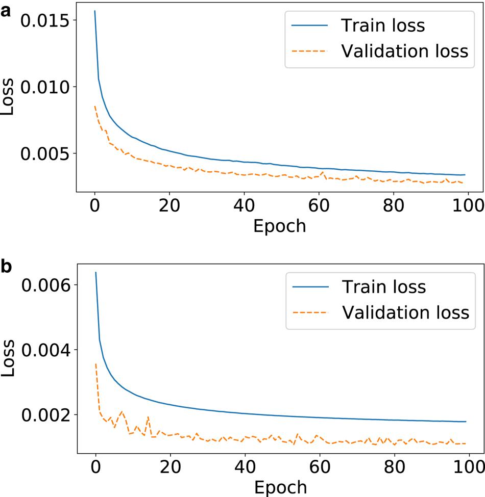
We conducted several experiments with various network parameters to seek for the optimal parameters in terms of model accuracy versus model evaluation costs. For that purpose, we split our dataset in two parts: one for training and one for validation. Appendix D shows the evolution of training and validation losses with respect to epochs. Unless specified differently, we always reserved Icefield A (resp. Aletsch and Rhone glacier with c = 12) for validation and take the others for training for icefield (resp. glacier) simulations. Note that the validation loss is always lower than the training loss demonstrating that our choice of validation data remains safely within the hull of the training dataset (Appendix D).
Fidelity
The fidelity is measured by taking the rescaled L 1 validation loss (Eqn. (4)) between the predicted ice flow field $\bar {\bf u}_{\rm P}$ and the reference one $\bar {\bf u}_{{\rm R}}$
 , as well as the L 1 relative error (taken only where the L 1 norm of the ice velocity is above 10 m a−1):

Table 1 displays the fidelity results of the trained ice flow emulator to reproduce the ice flow of Icefield A performed with PISM and of Aletsch glacier (with fixed sliding parameter c = 12) performed with CfsFlow varying network parameters such as the number of layers N lay, output filters N feat or kernel size N ker. It shows that increasing the number of filters N feat improves the fidelity of the solution. This is also true for the number of layers, however, only up to N lay = 16 layers as the fidelity deteriorates when deepening the network. Last, increasing the kernel size N ker from 3 (the most common value, see Fig. 4) does not improve the solution in all cases. Opting for large N lay, N ker and N feat numbers increases the number of network parameters, and thus the computational cost. Therefore, we selected two optimal parameter sets (one for each kind of dataset) that lead to fidelity levels above 90% while keeping low evaluation costs: (i) the parameter set (N feat, N ker, N lay) = (32, 3, 8) for PISM icefield data leads to a neural network that has ≈65 k trainable parameters (it stores into a 880 KB file), and (ii) the parameter set (N feat, N ker, N lay) = (32, 3, 16) for CfsFlow glacier data leads to a neural network that has ≈140 k trainable parameters (it stores into a 2 MB file).
Figures 9 and 10 compare the flow speeds of Icefield A and Aletsch glacier at the maximum ice extent to the reference simulations with the respective selected models. The fidelity of the emulated solution, compared to the reference PISM or CfsFlow solutions (which were not used in the training stage), is high and of the same order in all cases with mean relative errors below 9% (Table 1). This shows the neural network's ability to learn from data from different topographies and to apply this knowledge to new ones, even with a relative small model size (65 and 140 k of trainable parameters, respectively).
Vertically-averaged ice flow magnitude of Icefield A at its maximum state: PISM reference solution (a), IGM solution trained without (b) and with (c) the solution, and the difference between IGM and PISM solutions (d and e).

Vertically-averaged ice flow magnitude of the Aletsch glacier at its maximum state: CfsFlow reference solution (a), the IGM solution trained without (b) and with (c) the solution, and the difference between IGM and CfsFlow solutions (d and e).

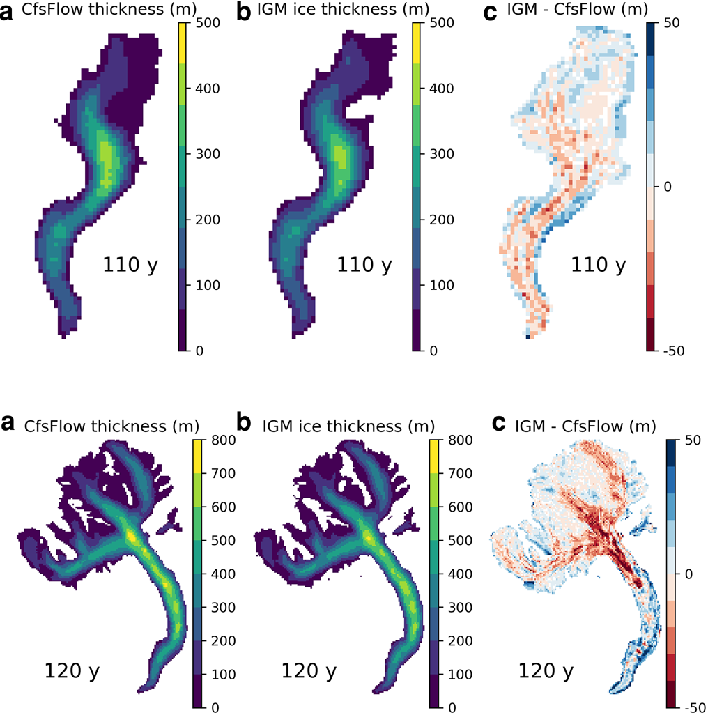
A closer look at the emulated ice flow field of Aletsch glacier (Fig. 10) shows that the ice flow is well reproduced for the three accumulation basins, however, larger discrepancies occur on the tongue and at Konkordiaplatz where the three tributary basins merge into a single tongue. While the training dataset generated by CfsFlow contains many examples of single channelized flow (Fig. 6), merging ice flows of similar sizes such as at Konkordiaplatz as well as thick ice (up to 800 m) is much less common in the training dataset, explaining why the flow in this region is less well reproduced than anywhere else. By contrast, single-branch and thinner valley glaciers such as Rhone Glacier are much more common and better represented in the training dataset. As a result (Fig. 11) the emulated ice flow is in better agreement with the reference CfsFlow one.
Vertically-averaged ice flow magnitude of the Rhone glacier at its maximum state: CfsFlow reference solution (a), IGM/test solutions (b), and the difference between IGM and CfsFlow solutions (c).

The L 1 error (or loss) between a predicted and a reference ice flow has two components, a ‘network’ component that measures the performance of the network to compress and recover solutions and a ‘data’ component that measures the error related to the abundance/lack of relevant training data. These two components can be distinguished by including the solution we wish to predict to the training dataset to measure the sole ‘network’ component (or compression error). Here we found that this error component is ${\sim }7\percnt$ in both cases, which is ${\sim }1\text {-}2\percnt$
 less than the L 1 original validation loss (${\sim }8\text {-}9\percnt$
 ). We therefore attribute the $7\percnt$
 to network errors and the remainder (${\sim } 1\text {-}2\percnt$
 ) to a lack of representative data. The reference solution, and the predicted solutions with or without the reference in the training are displayed in Figures 9 and 10. In the case of Aletsch glacier, the spatial error patterns show that including the reference solution in the training locally resolves the discrepancy at the convergence area (Konkordiaplatz) of the three ice flow branches (Fig. 10), confirming that this particular source of error mostly lies on the data side (i.e. the absence of analogues in the training dataset) unlike the remaining errors on the main glacier trunk.
Up to now, we have tested the learning of ice flow from different geometries, but leaving the sliding coefficient c unchanged (c = 12 km MPa−3 a−1). Table 2 gives the L 1 validation loss (m a−1) at the maximum extent of Rhone and Aletsch glacier simulations with different sliding coefficients c, including the values used for training {0, 6, 12, 25}, as well as intermediate values {3, 9, 18} to assess the interpolation accuracy. As a result, the values used for training yield to similar fidelity levels (${< }9\percnt$ ) while intermediate values yield to slightly deteriorated levels (${< }13\percnt$
 ).
).
L 1 validation loss (m a−1) and relative misfit (in %) defined by Eqn. (7) for Rhone and Aletsch glaciers with different sliding coefficients h including values that have been used for training (in bold), as well as intermediate values

Computational performance
Along with the fidelity results, Table 1 also displays the time needed to evaluate a single full ice flow field (after training) with the neural network and varying parameters using both computational resources of the same laptop (Thinkpad Lenovo P52): a GPU (NVIDIA Quadro P3200 GPU card with 1792 1.3 GHz cores) or a CPU (Intel(R) Core(TM) i7-8850H CPU with 6 2.6 GHz cores). For convenience, all CPU and GPU performance results given in this paper relate to this hardware. As a result, GPU and CPU show dramatically different performances. GPU always outperforms CPU (speed-ups between 2 and 8), however, the increasing computational cost coming from the model size and the domain resolution (larger for icefield than for glaciers) scales differently between GPU and CPU. While GPU and CPU have close performance for models with few trainable parameters and small domains, the GPU is especially advantageous for complex models (with many weights) and for large size domains.
While a key advantage of neural networks is their low evaluation cost, their training necessarily comes with substantial upstream computation costs, which must be invested for each set of ice flow settings. Table 3 lists these upstream costs for generating the data from traditional models and training the model itself. As a result, the generation of the full dataset was the most computationally expensive task: ≈7–26 days for icefield simulations with PISM and glacier simulations with CfsFlow on CPU, respectively, while the training of the optimal models took 8–24 h on GPU.
Computational costs required for the generation of all datasets on the CPU and for the training of the emulator on the GPU

Icefield and glacier evolutions
We now assess the fidelity and performance of the time-evolution model (Fig. 1) by replicating Icefield A, Aletsch and Rhone glacier transient simulations with IGM. It must be stressed that none of original Icefield A, Aletsch and Rhone glacier simulations were used for training IGM.
Fidelity
Overall, IGM shows good skill at reproducing ice thickness of Icefield A (Fig. 12), and Aletsch and Rhone glaciers at maximum ice extent (Fig. 13). The time-integrated root-mean-square error in terms of ice thickness is ≈20 m in all cases. IGM also reproduces the evolution of ice volume, ice extent and mean ice flow speed with high fidelity (Fig. 14) although small discrepancies arise, e.g. the ice flow of Aletsch Glacier is slightly overestimated with IGM. In the latter case, the cumulative errors remain very limited despite systematic errors in the ice flow (e.g. at the convergence area of the three ice flow branches, Fig. 10).
Maximum ice thickness of Icefield A modelled with PISM (a) and IGM (b), and the difference between the two (c).

Ice thickness fields of Rhone (top panels) and Aletsch (bottom panels) glaciers after 110 and 120 years with CfsFlow (a) and IGM (b), as well as the difference between the two (c).
Modelled evolution of ice volume, glaciated area and mean velocity field for Icefield A (a) and Aletsch glacier (b) simulations performed with IGM, PISM and CfsFlow.

Computational performance
Table 4 compares the computational times required for Icefield A and Aletsch glacier simulations with all models on CPU and GPU. Note that a direct comparison is only possible on CPU as none of PISM or CfsFlow runs on GPU. Additionally, we forced IGM to use a single core for comparison with CfsFlow as the latter only runs in serial. It must be stressed that the given speed-up does not include the training costs (data generation and training itself summarized in Table 3).
Overall computational time to achieve the simulation of Icefield A with PISM and IGM using CPU and GPU at 2 km resolution (top table) and of Aletsch glacier with CfsFlow and IGM using CPU and GPU (middle table). The bottom panel compares the computational times to simulate the retreat of Aletsch glacier for 150 years from today's state with another Stokes model Elmer/Ice and IGM, which was trained from Elmer/Ice simulations. The proportion of this time taken by the ice flow and mass-balance model components is additionally given when they are significant
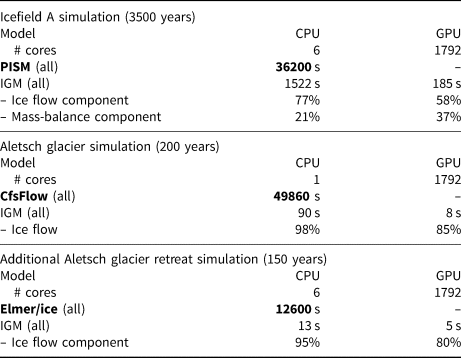
Table 4 shows that IGM outperforms PISM for the Icefield A simulation by a factor of ~20 on CPU, with an additional ~ 10 × speed-up on GPU. Here, the high resolution of the icefield computational domain (512 × 512) takes full advantage of the parallelism and explains the superiority of the GPU over the CPU. Note that while most of the time is taken by the ice flow model in glacier simulations, the PDD mass-balance model (Appendix B) in the icefield simulation requires significant aside computational effort (even on the GPU) as it loops over each grid cell at short time-scale intervals.
On the other hand, IGM outperforms CfsFlow for the simulation of Aletsch Glacier by a factor of ~600 on CPU (using a single core), with an additional ~ 10 × speed-up on GPU, but only ~ 2 × when comparing to a six-core CPU run (not shown). Here, the GPU remains superior due to the large size of the Stokes ice flow neural network as noted before, however, the added value is less important than before as the size of the computational domain is much lower (185 × 121). As an additional benchmark in Table 4, we have compared the computational time to simulate the full retreat of Aletsch glacier for 150 years from today's state with another Stokes model – Elmer/Ice (Gagliardini and others, Reference Gagliardini2013) – and IGM, which was trained from Elmer/Ice simulations. As a result, we found a ~ 1000 × speed-up when comparing IGM and Elmer/Ice runs on CPU (both using all six cores), with an additional speed-up of ~ 2 × on GPU.
Discussion
In ice flow modelling, the choice of a stress balance model is often the result of a compromise between mechanical complexity, spatial resolution and computational affordability. Shallow models rely on simplifications to make them computationally tractable but at the expense of mechanical loss of accuracy (e.g. Greve and Blatter, Reference Greve and Blatter2009). In contrast, the Stokes model is computationally expensive, and it is therefore challenging to use it for large domains and long time scales. The transfer of these models directly to GPUs offers promising speed-ups (Räss and others, Reference Räss, Licul, Herman, Podladchikov and Suckale2020), however this usually requires a full reimplementation of the numerical model. As an added value to traditional modelling, our results demonstrate that substituting a well-trained neural network emulator running on GPUs for a traditional hybrid or Stokes solver permits to speed up by several orders of magnitude if one excludes a minor loss in accuracy and training costs, which are invested a single time for a given ice flow setting.
Network compression capability
We find that a relatively simple CNN composed of tens of layers is capable of learning from realizations of two ice flow models of different complexity levels and of retrieving composite solutions with high and similar fidelity (above 90%) with respect to the instructor models. The model size in terms of trainable parameters (105–106) – or equivalently in terms of data storage (1–2 MB) – is very small compared to the amount of data that was used for training (above 1 GB). The misfit between emulated and reference solutions due to the neural network itself (i.e. the compressibility error) is close to 7–8% for the emulation of both CfsFlow and PISM. This is likely much smaller than data and model uncertainties for many glaciological applications. By contrast, the error related to the richness of the dataset to include a large diversity of relevant dynamical states is fairly small (${< }2\percnt$ ). This therefore demonstrates the ability to learn the relationship between topographic and ice flow variables in a generic manner, i.e. to translate the knowledge acquired on some glaciers to others. Most importantly, a model as complex as the 3-D Stokes equations can be learnt and emulated very efficiently by a neural network, which maps 2-D fields.
Because using standard network parameters already results in a high fidelity emulator, we have not explored further parameter choices, thus leaving room for future improvements. For instance, we used the L 1 norm as our loss function, which is a common choice in deep learning accelerating CFD (Kim and others, Reference Kim, Azevedo, Thuerey, Kim, Gross and Solenthaler2019; Thuerey and others, Reference Thuerey, Weißenow, Prantl and Hu2020), future studies could explore other loss/misfit functions such as L 2, L p, … or other gradient-based norms such as W 1,p with p = 1 + 1/n, which is the natural norm in which to analyse the existence and uniqueness of solutions of the Stokes problem in its variational (or minimization) form (Jouvet and Rappaz, Reference Jouvet and Rappaz2011).
Optimality of the dataset
We have found that our original dataset made of arbitrarily chosen glacier/valley topographies to train IGM was far from optimal (e.g. containing redundant data). Criteria for the optimality of the dataset (in terms of model fidelity to data size) were investigated. First, we attempted (not shown) to use principal component analysis to preprocess and reduce the dimensionality of data while preserving the original structure and relevant relationships (e.g. Brinkerhoff and others, Reference Brinkerhoff, Aschwanden and Fahnestock2021). However, our iterative selection scheme was found to be more efficient to filter non-relevant data: the glacier dataset was reduced by ≈75% without affecting the emulator accuracy.
Varying basal sliding conditions
Real-world glacier modelling requires the tuning of ice flow parameters to observational data. For that purpose, our Stokes emulator can take the basal sliding coefficient as input thanks to an exploration of this parameter in the training dataset. Our results have shown that the interpolation errors between the training states remain fairly low (Table 2). Note that while we used spatially constant sliding coefficients for training, our emulator can take a spatially variable sliding coefficient (e.g. resulting from surface data assimilation) as input field. In such a case, it would be desirable to assess the emulator accuracy against reference solutions based on spatially sliding coefficients to evaluate whether the training data should be augmented with such solutions.
Embedding into the time evolution model
While even a small ${< }10\percnt$ inaccuracy of the ice flow emulator could raise concerns of cumulative errors in the time evolution model due to the feedback between ice flow and elevation-dependent mass balance, the good match between time evolution variables (Figs 12–14) suggests instead that the errors compensate. Additional investigations have shown that the errors of the divergence of the ice flux (not shown), which matters in the time-advancing scheme, are much more unevenly distributed than ice flow errors, leading to probable error compensation. This suggests that embedding our neural network emulator iteratively into the mass conservation equation is a safe operation, which keeps a high level of fidelity.
Speed-ups
The significant speed-up obtained here is the combined result of two key ingredients: (i) neural networks (once trained) are very cheap compared to the direct solving of non-linear diffusion equations describing the ice flow; (ii) the evaluation of such a neural network, as well as other expensive IGM model component tasks (like the PDD mass balance) runs well in parallel and can therefore take advantage of GPUs. Our performance results demonstrated that (i) a direct speed-up of ≈20 and 600–1000 for hybrid and Stokes mechanics on our examples related to CPUs, (ii) GPU can give another substantial speed-up, which is harder to quantify as it depends on modelling features and GPU performance. Indeed, GPUs outperform CPUs in general for large computations when all GPU cores available are used. Here, GPUs will show great advantage when the neural network size is large (such as the one selected to emulate Stokes) or/and when the size of the modelled domain is high. We can therefore anticipate a great added value of GPU for emulating Stokes and/or large size computations (e.g. the modelling of large ice sheets in high resolution). Finally, we used here a single laptop integrated GPU card (NVIDIA Quadro P3200 GPU), which features moderate performance (<2000 1.3 GHz cores and 6 GB of memory). There is therefore room for further speed-up by switching to the latest available GPUs, considering that the price performance of GPUs currently doubles roughly every two years.
Advantages and limitations of IGM
Besides the computational efficiency to obtain the ice flow solution at near Stokes accuracy, IGM has a certain number of practical advantages:
(1) Although it can be trained on 3-D ice flow models, IGM deals with 2-D regular grids facilitating the management of input and output data.
(2) IGM only takes gridded bedrock and surface elevations as topographic inputs, and does not require to identify any catchment or centre flow line, in contrast to flowline-based models.
(3) IGM users can directly do simulations by picking already trained model emulators (which vary according to spatial resolution) from a model collection library that comes along IGM's code.
(4) Although IGM performs better on GPU, it runs across both CPU and GPU, and switching from one to another architecture is trivial.
On the other hand, IGM has the following limitations, which call for further development:
(1) One must keep in mind that the applicability of IGM is dictated by the dataset used for training the emulator. For instance, the CfsFlow-trained emulator presented here will not be able to model the ice flow of glaciers, whose dimensions exceed the hull defined by the set of training glaciers (Fig. 6).
(2) The current emulator assumes isothermal ice for simplicity, i.e. it ignores the effect of ice temperature on ice deformation and basal sliding.
(3) In our approach, we have natural inflow and outflow conditions at the border of the computational domain, and no specific other boundary conditions can be prescribed.
(4) IGM's ice flow emulator works only with regular gridded data, and using unstructured meshes is incompatible with this strategy.
Perspectives
Potential for applications
The computational efficiency of IGM opens perspectives in paleo ice flow modelling, which involves very long time scales and relatively high-resolution computational domains such as: (i) the simulation of large icefields for multi-glacial cycles for reconstruction purposes (Seguinot and others, Reference Seguinot2018) or to study glacial erosion and landscape evolution (Egholm and others, Reference Egholm2017) – an application that requires high-order mechanics to capture basal sliding, (ii) the inference of paleo climatic patterns from geomorphological evidence using an inverse modelling (Višnjević and others, Reference Višnjević, Herman and Prasicek2020).
The ability of IGM to learn ice mechanics from an ensemble of glaciers simulated with a state-of-the-art physical instructor model and translate knowledge acquired from some glaciers may also be exploited in global modelling. Indeed, today's global models all rely on highly simplified SIA-based models contributing to model uncertainties. Providing a training set over a representative sample of glaciers with a range of ice flow parameters, IGM would permit to model a massive number of glaciers with a near Stokes accuracy.
Generalizing the emulator
It is straightforward to generalize our CNN (Fig. 3) with further relevant spatially variable inputs (e.g. ice hardness) to emulate a more generic ice flow model. In the same way, adding information on buoyancy as input would permit to learn from an ice shelf dynamical model, and then generalize the emulator to floating ice. Instead, the main challenge here is to provide a larger ensemble of training data.
Data assimilation
While the current paper focussed on emulating a cheap ice flow emulator from a mechanical model, it does not overcome the necessary step of calibrating ice flow parameters to observational data. Besides their low computational evaluation costs, neural networks rely on automatic differentiation, which is a strong asset for inverse modelling. The optimization of basal conditions (bedrock location and basal sliding) from surface observations through the inversion of an ice flow emulator such as the one we used should be investigated.
In contrast, training a network similar to ours with real observations is a tempting alternative to directly include data assimilation. However, this strategy comes with a number of challenges that should be tackled, including (i) the availability of abundant observational data necessary for training a deep network (especially for the ice thickness) (ii) the embedding of possibly contradictory observational data (explaining real ice flow requires more than ice thicknesses and surface slopes, i.e. basal data which are hard to observe) and (iii) the effect of the data noise due to contradictory observational data on the iterative time evolution scheme. Future research is therefore needed to explore this potential.
Conclusions
We have introduced a new type of glacier model, which computes the ice flow using a deep learning emulator trained from hybrid SIA + SSA or Stokes mechanical models. Our strategy permits us to compress the dynamical states produced by these models and to use this information to substitute the expensive ice flow model by a cheap emulator and therefore speed up the overall time evolution model considerably. We have demonstrated that the resulting model IGM, after appropriate training, models the flow and evolution of large icefields over millennia and of individual mountain glaciers over centuries up to 20 and 1000 faster than traditional hybrid and Stokes on CPUs with fidelity levels above 90%, and up to 200 and 2000 faster by switching to GPUs. IGM has potential for application in global glacier modelling as well as in paleo and modern ice-sheet simulations. The IGM code and the trained ice flow emulators are publicly available at https://github.com/jouvetg/igm.
Acknowledgements
We acknowledge Ed Bueler, Fabien Maussion and an anonymous referee for their valuable comments on the original manuscript. We are thankful to Constantine Khroulev and Olivier Gagliardini for support with PISM and Elmer/Ice, respectively. The Python code PyPDD by J. Seguinot has greatly helped the integration of the PDD model in IGM. The emulator was originally motivated to speed-up an ice flow model within the framework of project 200021-162444 supported by the Swiss National Science Foundation (SNSF). Michael Imhof is acknowledged for providing the script that served to produce Fig. 5.
Author contributions
G.J. conceived the study, performed the simulations, designed the ice flow emulator with support from G.C. and B.K., wrote the paper with support from all co-authors, and wrote the IGM code with contributions and support from G.C. for the Tensorflow implementation.
Appendix A: Solving mass conservation
The mass conservation equation (1) is solved using a first-order upwind finite-volume scheme similar as the one described in Lipscomb and others (Reference Lipscomb2019). Here we use a staggered grid, i.e. the ice thickness is defined at the centre of each grid cell, but the ice flow velocities used in the scheme are defined at the middle of the grid edges by a simple averaging. The key advantage of using such a staggered grid is that solving Eqn. (1) by finite volumes becomes natural as mass of ice is allowed to move from cell to cell (where the thickness is defined) from edge-defined fluxes (inferred from depth-average velocities). The transport of mass is governed following an upwind scheme for stability reasons. The resulting scheme is fully explicit (and therefore runs well in parallel), however, subject to CFL condition (2). Further details about this scheme can be found in Lipscomb and others (Reference Lipscomb2019, Section 5.5.3).
Appendix B: Icefield simulations with PISM
To generate icefield simulation data, we selected five 1024 km × 1024 km tiles of existing topographically diverse mountainous environments worldwide (Table 5 and Fig. 5). For each tile, we extracted the publicly available NASA Shuttle Radar Topographic Mission (SRTM, http://srtm.csi.cgiar.org/) Digital Elevation Model (DEM), resampled at 2 km resolution to be used as basal topography in PISM. Details about the ice flow and mass-balance models used in PISM are now described in turn:
(1) Basal sliding was modelled with law (6) with parameter c = 70 km MPa−3 a−1, which was chosen so that a basal shear stress of 80 kPa corresponds to a sliding velocity of ≈35 m a−1 (Pattyn and others, Reference Pattyn2012).
(2) Surface mass balance (difference between accumulation and ablation) is calculated from the monthly mean surface air temperature, monthly precipitation and daily variability of surface air temperature. Accumulation is equal to solid precipitation when the temperature is below 0°C, and decreases to zero linearly between 0 and 2°C. Ablation is computed proportionally to the number of positive degree days (Hock, Reference Hock2003) with factors f i = 8 mm K−1 d−1 w.e. for ice and f s = 3 mm K−1 d−1 w.e. for snow, which are taken from the EISMINT intercomparison experiments for Greenland (MacAyeal, Reference MacAyeal1997).
As today's climate forcing, we took the monthly temperature and precipitation from the WorldClim dataset (Fick and Hijmans, Reference Fick and Hijmans2017). Starting from ice-free conditions, we linearly decreased temperature at a rate of 1°C per century until a large icefield covering the tile was built. Then, the cooling was reversed symmetrically into warming at the same rate until the ice has completely disappeared.
List of tiles used to generate icefields simulations with PISM at 2 km resolution. The longitude and the latitude correspond to the location of the centreof each squared tiles

Appendix C: Glacier simulations with CfsFlow
To generate glacier simulation data, we have picked 41 diverse existing valleys from the European Alps and from New Zealand with drainage basins ranging from 80 to 700 km2. For each one, we have extracted the publicly available NASA Shuttle Radar Topographic Mission (SRTM, http://srtm.csi.cgiar.org/) Digital Elevation Model (DEM) to be used as bedrock, and built a 100 m resolution two-dimensional structured mesh of the DEM. A three-dimensional mesh was then vertically extruded with 100 of 10 m thick layers. In more detail, we use CfsFlow with the following specific settings:
(1) Basal sliding was modelled by (6) with constant coefficient c taken among {0, 6, 12, 25, 70} km MPa−3 a−1.
(2) As mass balance, we use a simple parametrization based on given Equilibrium Line Altitude (ELA) z ELA, accumulation β acc and ablation β abl vertical gradients, and maximum accumulation rates a max:
$${\rm SMB}( z) = \left\{\matrix{ \min( \beta_{{\rm acc}} ( z - z_{{\rm ELA}}) ,\; a_{{\rm max}}) ,\; \hfill & \text{if } z \geq z_{{\rm ELA}} \hfill \cr \beta_{{\rm abl}} ( z - z_{{\rm ELA}}) ,\; \hfill & \text{otherwise.} \hfill }\right.$$with β abl = 0.009 a−1, β acc = 0.005 a−1, and a max = 2 m a−1.

We initialized the model with ice-free conditions. For the first 100 years, the ELA was chosen constant with the 20% quantile value of the original glacier top surface elevation to allow for glacier advance. For the next and last 100 years, the ELA was raised linearly until it reached the 90% quantile value of the original glacier top surface elevation to allow for glacier retreat.
Appendix D: Learning curve
Figure 15 shows the learning curve, i.e. the evolution L 1 loss/misfit function against the number of epochs (an epoch corresponds to one pass over the entire training dataset), during the training of the two datasets. As a result, the convergence of the training was always found efficient and fairly smooth. The validation loss was always found below the training loss.
Evolution of the train and the validation loss while training the ice flow emulator from the data generated with PISM (top) and CfsFlow (bottom).
Appendix E: Digest of artificial neural networks
Artificial neural networks approximate a mathematical function that maps input to output variables through a sequence of layers that contain nodes (or neurons). Mathematically, the output of each neuron is computed by some non-linear function (called activation) as the sum of its inputs. Neurons and connections have weights that are adjusted during the training (i.e. learning) stage. The optimal weights of the network are found by minimizing a certain cost function (often referred as loss function), which is most often defined as the misfit between the ground truth of the training data and the output of the network. As the number of weights of an effective neural network can be very high (typical 106 − 108), the availability of a large data set is the key to determine the optimal weights and prevent against underdetermined systems. The optimization (or training) of the neural network often relies on a batch gradient descent method, which consists of sequentially adjusting weights by computing descent directions on small subsets (called batches) of the training data from the error between the model and data outputs. While the model evaluation happens sequentially from the first to the last layer (feed forward), the training happens sequentially in the opposite direction (back propagation) from the error computed at the last stage to the first input layer. In that case, the gradients required to optimize each weight are computed by the simple chain rule for derivatives. We refer to LeCun and others (Reference LeCun, Bengio and Hinton2015) for an in-depth review on deep learning.


 Open access