


Introduction
The ice sheets are the biggest freshwater reservoirs of the earth system and thus are a significant factor for the future evolution of sea level (Stocker and others, Reference Stocker2013; Shepherd and others, Reference Shepherd2019; Tapley and others, Reference Tapley2019; Edwards and others, Reference Edwards2021). Thus, understanding the behaviour of the ice sheets in response to changes in climate is essential for improving predictions for the future projections. Radio-echo sounding (RES) of ice and the mapping of internal reflections can provide valuable insights into the history of ice streams, accumulation patterns and the physical properties of internal layers in Greenland and Antarctica (e.g. Fujita and Mae, Reference Fujita and Mae1994; Fujita and others, Reference Fujita1999; Eisen and others, Reference Eisen, Hamann, Kipfstuhl, Steinhage and Wilhelms2007; Urbini and others, Reference Urbini2008; Rodriguez-Morales and others, Reference Rodriguez-Morales2014; MacGregor and others, Reference MacGregor2015; Cavitte and others, Reference Cavitte2016, Reference Cavitte2018; Winter and others, Reference Winter2017; Kjær and others, Reference Kjær2018; Schroeder and others, Reference Schroeder2019). Investigating physical properties of ice sheets and understanding complex ice flow behaviours (e.g. effects from anisotropy) can provide more insights to acquire missing process knowledge of ice stream dynamics in the ice sheet and glacier models. The speed of flow in the anisotropy of the ice is faster than isotropic ice, thus, anisotropic ice can enhance the speed of flow (Glen, Reference Glen1958; Thorsteinsson and others, Reference Thorsteinsson, Waddington, Taylor, Alley and Blankenship1999). Most ice-sheet and glacier models assume the ice to be isotropic. Therefore, understanding ice flow behaviours can thus reduce model uncertainty and increase prediction accuracy for the future behaviour of sea level projections.
Together, the three locations comprise the three main dynamic flow regimes in northern Greenland: divide, flank and streaming flow. An overview of the Greenland ice core sites in relation to the dynamic setting of the Greenland Ice Sheet is shown in Figure 1. The drill site of the North Greenland Eemian (NEEM) core, which provided the oldest reconstructed record from folded layers in a core (Dahl-Jensen and others, Reference Dahl-Jensen2013), is located on the north-eastern ice divide of Greenland. The North Greenland Ice Core Project (NGRIP) yielded an ice core with the oldest undisturbed record in Greenland back to 122 ka b2k (years before the year 2000 CE) (Wolff and others, Reference Wolff, Chappellaz, Blunier, Rasmussen and Svensson2010). It is located on the central divide, about 200 km west-southwest of the East Greenland deep Ice-core Project (EGRIP) drill site, where flow velocities are about 1.3 m a−1. The drill site of the EGRIP is located in the region of the NEGIS, where the ice is currently moving at ~55 m a−1 to the north–northeast (NNE) (Hvidberg and others, Reference Hvidberg2020).
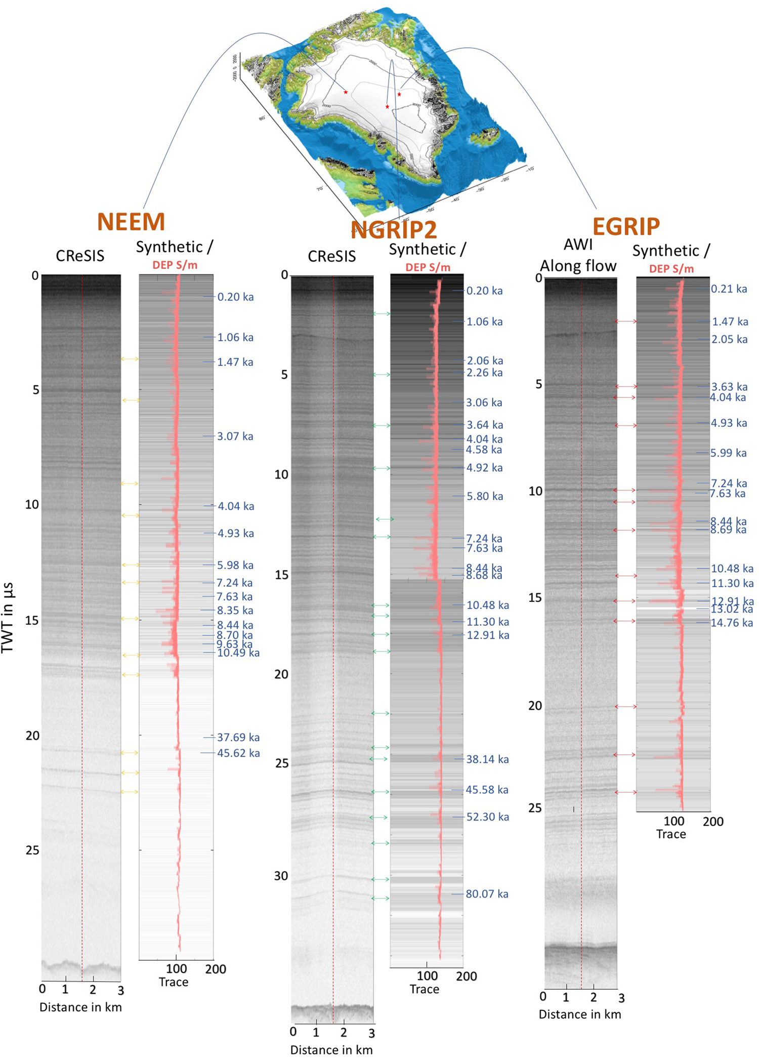
(a) Locations of deep ice-core drill sites in Greenland Ice Sheet. (b) Focus on ice core locations in the vicinity of NEGIS and northern Greenland used in this study. (c) NEEM drill site with the RES profile line from CReSIS flight 20110329_02_028. (d) NGRIP drill site with the RES profile line of CReSIS flight 20120330_03_014. (e) EGRIP drill site with the RES profile line of AWI flights 20180508_06_004 and 20180512_01_001. The red crosses mark the traces closest to each drill site which we use in our analysis (single traces in Fig. 2). The red cross on the cross-flow line at EGRIP in panel (e) is the closest point to the drill site based on the space between each trace that is 15 m for the AWI radar measurement. The panels (c) and (e) are strongly zoomed in (scale bar in meters), compared to panel (d) with the scale bar covering a few km. Colours show surface flow velocities from satellite data (Joughin and others, Reference Joughin, Smith and Howat2018). Projection: WGS 84/NSIDC Sea Ice Polar Stereographic North (EPSG:3413).

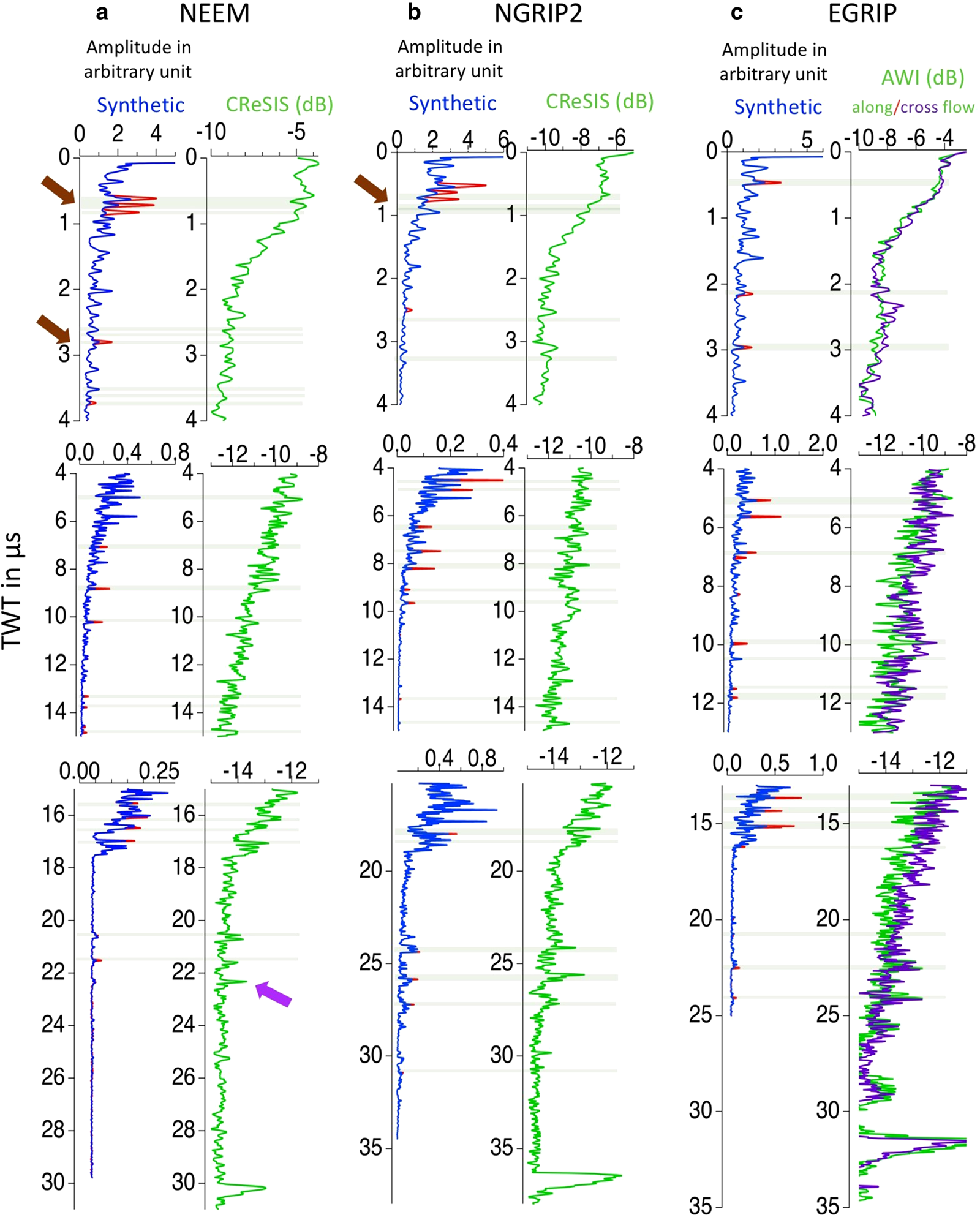
A-scopes for traces of the radar systems (green) at (a) NEEM, (b) NGRIP2 and (c) EGRIP (along-flow in green and cross-flow in purple (positions indicated by red crosses in Fig. 1)) and the synthetic traces (blue). The surface reflection of each trace is shifted to time zero. The reflections used for synchronization are marked by grey bands. The synthetic peaks highlighted in red cause the identified dated reflections (Table 3) which are observed both in the synthetic and RES traces. The coloured arrows highlight IRHs that are described in detail in the Results section. For better graphical representation, we split each trace into three TWT intervals, as the amplitude decays with depth.
The matched layers of synthetic and real radargrams with TWTs at the ice core sites, depth ranges of their reflecting conductivity/permittivity sections of DEP and corresponding ages from the GICC05 (depth, age) timescale taken from Mojtabavi and others (Reference Mojtabavi2020) and Rasmussen and others (Reference Rasmussen2013).

To understand the interplay between the catchment areas and their outflow, we need to study regions of increased ice flow velocities. The Northeast Greenland Ice Stream (NEGIS) is the largest ice stream in Greenland, draining about 12% of the Greenland Ice Sheet (Fahnestock and others, Reference Fahnestock, Bindschadler, Kwok and Jezek1993, Reference Fahnestock2001; Vallelonga and others, Reference Vallelonga2014; MacGregor and others, Reference MacGregor2015; Joughin and others, Reference Joughin, Smith and Howat2018; Larsen and others, Reference Larsen2018). The drill site of the EGRIP is located in the region of the NEGIS, where the ice is currently moving at ~55 m a−1 to the NNE (Hvidberg and others, Reference Hvidberg2020). The ice-dynamic regime of the NEGIS is complex and, interpolating the surface velocity into depth, all ice entering the ice stream seems passing through its well developed shear margins (Christianson and others, Reference Christianson2014; Franke and others, Reference Franke2020a).
Over the past 20 years, multi-channel ultra-wide band (UWB) radar systems (MacGregor and others, Reference MacGregor2015; Hale and others, Reference Hale2016; Franke and others, Reference Franke2020b) have provided high-resolution data sets, and offered opportunities to understand the physics of internal stratigraphy from the local scale to large areas of the ice sheet. Synthetic modelling of RES data has previously been applied to the Greenland and Antarctic records from the GRIP ice core, EPICA Dome C (EDC) and the EPICA Dronning Maud Land (EDML) ice cores (Hempel and others, Reference Hempel, Thyssen, Gundestrup, Clausen and Miller2000; Eisen and others, Reference Eisen, Nixdorf, Wilhelms and Miller2004, Reference Eisen, Wilhelms, Steinhage and Schwander2006; Winter and others, Reference Winter2017). Winter and others (Reference Winter2017) used this technique to compare data in the vicinity of EDC, where they investigated how different radar systems image changes from physical properties in internal reflection horizons (IRHs) and the differences of the radar systems in bed topography, penetration depth and capacity of imaging the basal layer. Applying a comparable approach to Greenland radar records will help to understand the physical properties and thus inform ice flow models as well as contribute to process understanding of ice dynamics. Combining the local results from modelled radargrams, on the basis of ice core data from different regimes, with the IRHs in regionally distributed profiles of airborne RES provide the opportunity to upscale local measurements of physical properties. Most IRHs in the ice sheet can be considered isochrones (Siegert and others, Reference Siegert, Hodgkinst and Dowdeswell1998; Fujita and others, Reference Fujita1999; Eisen and others, Reference Eisen, Wilhelms, Nixdorf and Miller2003; Cavitte and others, Reference Cavitte2016). Therefore, combining the synthetic radar modelling with a depth–age relationship form the northern Greenland ice cores (Rasmussen and others, Reference Rasmussen2013; Mojtabavi and others, Reference Mojtabavi2020) can allow the dating of the IRHs in northern Greenland.
Regarding the physical origin of IRHs, conductivity can explain the majority of the radar returns in ice sheet (Fujita and others, Reference Fujita1999; Hempel and others, Reference Hempel, Thyssen, Gundestrup, Clausen and Miller2000; Miners and others, Reference Miners, Wolff, Moore, Jacobel and Hempel2002; Eisen and others, Reference Eisen, Wilhelms, Steinhage and Schwander2006). In general, it can be stated that for the upper ~100 m of ice sheet, the reflections are mostly based on permittivity and density contrasts (Paren and Robin, Reference Paren and Robin1975; Arcone and others, Reference Arcone, Spikes, Hamilton and Mayewski2004; Eisen and others, Reference Eisen, Nixdorf, Wilhelms and Miller2004). Below 100 m depth, the variability of the density-based permittivity decreases and reflections dominated by permittivity contrasts which are in few cases related to changes in crystal orientation fabric (COF), which affects the real part of permittivity (Eisen and others, Reference Eisen, Hamann, Kipfstuhl, Steinhage and Wilhelms2007). The deformation of an ice crystal depends on the direction and magnitude of stress and strain in the ice sheet (Gusmeroli and others, Reference Gusmeroli, Pettit, Kennedy and Ritz2012; Faria and others, Reference Faria, Weikusat and Azuma2014; Llorens and others, Reference Llorens2016; Qi and others, Reference Qi2019). Random orientation of all ice crystals indicates the COF is isotropic. If a large number of c-axes align (e.g. parallel), it results in an anisotropic COF (Gusmeroli and others, Reference Gusmeroli, Pettit, Kennedy and Ritz2012). In some cases, IRHs can be caused by sudden changes in COF. Anisotropy-derived IRHs will be characterized either by polarization-dependent variations in the wave propagation speed or by anisotropic backscatter. The anisotropy in terms of permittivity of a monocrystal of ice has been determined as Δɛ′ = 0.34 (Matsuoka and others, Reference Matsuoka, Fujita, Morishima and Mae1997). For an anisotropic fabric, the size of fabric eigenvalues and orientation of eigenvectors determine the effective permittivity and thus wave speed in a particular polarization plane.
As the first step, we apply a numerical model for electromagnetic wave propagation (Eisen and others, Reference Eisen, Nixdorf, Wilhelms and Miller2004) to records of dielectric properties to calculate synthetic radargrams. Dielectric observations are taken from the three northern Greenland deep ice cores: EGRIP, NEEM and NGRIP. We compare the synthetic radargrams and the multi-channel UWB radar data in order to match common IRHs between airborne RES data and synthetic radargrams and identify the physical processes that cause the reflections (i.e. the physical properties of a certain IRH). As a second step, we determine ages for the reflectors that can be considered as isochrones. The IRHs are assigned ages from the depth–age relationship (Rasmussen and others, Reference Rasmussen2013; Mojtabavi and others, Reference Mojtabavi2020) of the northern Greenland ice cores. Finally, for the EGRIP drill site, we also investigate polarization-dependent traveltime differences in the ice stream to infer the potential distribution of the anisotropic fabric.
Method
Airborne radar data
In May 2018, the Alfred Wegener Institute (AWI) collected the extensive airborne radar survey EGRIP-NOR-2018 on the NEGIS in the vicinity of the EGRIP drill site with an eight-channel radar system (MCoRDS5) mounted on AWI's Polar6 aircraft (Franke and others, Reference Franke2021). The EGRIP drill site (75.38°N, 35.60°W) and the location of selected RES profiles that are located along the upstream part of the NEGIS are shown in Figure 1e. The radar sounder was developed at the Centre for Remote Sensing of Ice Sheets (CReSIS) at the University of Kansas and was designed for sounding ice thickness, internal layering and the basal unit of ice sheets. A detailed description of the radar system is given by Hale and others (Reference Hale2016) and Franke and others (Reference Franke2020b). The radar system uses different transmit pulse durations as well as different receiver gains for different parts of the ice column to increase the dynamic range of the system. The recording parameters for the survey are shown in Table 1. For the comparison with the synthetic radargrams we use a single trace from the SAR processed data product of the EGRIP-NOR-2018 campaign (for details of the survey see Franke and others, Reference Franke2020b, Reference Franke2021). The main processing steps of the UWB radar data include presumming (incoherent averaging) during RES data acquisition, pulse compression, f-k migration-based SAR processing as well as channel and waveform combination during the processing (for more details see Franke and others, Reference Franke2020b). The diameter of the Fresnel zone is ~60 m based on the bandwidth of 180–210 MHz and the ice thickness range of 2–3 km (Franke and others, Reference Franke2020a). The SAR processing algorithms compute a one-dimensional layered dielectric model, based on the location of the ice surface, with a dielectric constant of 3.15 for ice (Rodriguez-Morales and others, Reference Rodriguez-Morales2014). For details of the radar processing see Rodriguez-Morales and others (Reference Rodriguez-Morales2014) and Franke and others (Reference Franke2020b). We selected the traces closest to the EGRIP drill site from one profile oriented along ice-flow direction (profile 20180512_01_001) and a second profile oriented across ice-flow direction (profile 20180508_06_004) (Fig. 1). The distance of the traces oriented along and across ice flow to the EGRIP drill site is ~30 and ~12 m respectively.
Summary of the RES systems and modelled data.

The NEEM and NGRIP drill sites are shown in Figure 1, panels c and d. For comparison of the synthetic radargrams at the location of the two ice cores, we used two radar profiles (profile 20110329_02_028 for NEEM and profile 20120330_03_014 for NGRIP) from the operation ice bridge (CReSIS, 2016). We used the ‘csarp_standard’ data product, which represents SAR processed radar data downloaded from the CReSIS website (www.cresis.ku.edu). The recording parameters for the survey around the NEEM and NGRIP with the Multi-Channel Coherent Radar Depth Sounder (MCoRDS2) mounted on NASA's P-3 aircraft are shown in Table 1. A detailed description of the CReSIS data product and processing parameters is available on the CReSIS website. The closest trace's distance to the NEEM drill sites is ~34 m, while the closest trace distance to the drill site of the NGRIP core is ~2.75 km (Fig. 1). To compare the measured airborne RES data with the modelled synthetic data, we shifted the zero time of the airborne RES data to the surface reflection (air–ice interface). In this way, the RES data and synthetic trace surfaces are aligned.
Dielectric profiling (DEP) and ice core data
The dielectric properties (Moore and Paren, Reference Moore and Paren1987) of the EGRIP, NEEM and NGRIP ice cores were obtained with a DEP (dielectrical profiling) bench at a frequency of 250 kHz and a vertical resolution of 5 mm as described by Wilhelms and others (Reference Wilhelms, Kipfstuhl, Miller, Heinloth and Firestone1998), Wilhelms (Reference Wilhelms1996, Reference Wilhelms2005), Mojtabavi and others (Reference Mojtabavi2020). To yield the best possible interpretation of the DEP data, ice core breaks, missing pieces and differing overall quality of the ice core sections were logged during the processing. Slight capacitance/conductance variations due to deformation of the cables of the DEP device were corrected by the use of calibration data. A detailed description of DEP data processing of the EGRIP, NEEM and NGRIP ice cores is given by Mojtabavi and others (Reference Mojtabavi2020). At the time of this study, the EGRIP drilling campaign has not yet reached bedrock, therefore we present and analyse only the available DEP data, which correspond to the upper ~2122 m of the ice column that were profiled during the 2017–19 field seasons. For the NEEM core, we supplemented the topmost 100 m of the main core record with the NEEM-2008-S1 firn core record (Karlsson and others, Reference Karlsson2016) which originates from the NEEM access hole. The DEP data of the main NEEM ice core reach down to a depth of ~2537 m, which is about 20 m above the bedrock, and were recorded over several field seasons between 2008 and 2012. As the first NGRIP coring (here referred to as ‘NGRIP1’) terminated at ~1372 m depth due to a jammed drill, a second hole was restarted a few metres away, here referred to as ‘NGRIP2’. The DEP data from the NGRIP2 ice core reach down to 2930 m and were measured during the 1998–2004 field seasons. The data from the upper part of NGRIP2 down to 1298.705 m are published in this study for the first time, while data from the deeper part were presented by Rasmussen and others (Reference Rasmussen2013). Table 2 summarizes the unpublished and published DEP data sources used in this study.
Summary of the DEP data sets.

It should be noted that all DEP data are not corrected for the temperature difference between the deep ice in-situ and during the measurements in the field. However, according to Winter and others (Reference Winter2017), temperature should not alter the signature of conductivity and permittivity reflection patterns, as temperature affects the amplitude of the reflections which has no incidence on the depth of IRHs which is the main parameter of our comparison. The ice cores are drilled in a trench, which implies that the DEP records start at a depth of 13.77, 6.55 and 11.02 m for the EGRIP, NEEM and NGRIP2 ice cores, respectively. To compare modelled and observed results, we extrapolate the DEP data up to the surface, using a relative permittivity of 1.55 and an electric conductivity of 4 μS m−1 as surface values (Winter and others, Reference Winter2017). The values are the density and conductivity mixed permittivity (DECOMP) (Wilhelms, Reference Wilhelms2005) of the measured pure ice conductivity (20 μS m−1), the assumed surface firn density (300 kg m−3) and the ordinary relative pure ice permittivity (3.15), as determined below.
Modelling of synthetic radar traces and the depth of IRHs
Following the approach in Winter and others (Reference Winter2017), we used the conductivity and permittivity records, measured through DEP as described above as input for the 1D-FDTD numerical model (One-Dimensional Finite Difference Time Domain) ‘emice’ (Eisen and others, Reference Eisen, Nixdorf, Wilhelms and Miller2004) to calculate synthetic radar traces. A detailed description of the calculation and calibration to the DEP data is given by Mojtabavi and others (Reference Mojtabavi2020). Following Eisen and others (Reference Eisen, Wilhelms, Steinhage and Schwander2006), we tested different wavelets and chose a Ricker wavelet for this study, which is short and thus favourable to determine the depth of the reflectors’ origin at high resolution. The envelope of the synthetic traces, which is related to the reflected energy, is obtained by applying a Hilbert magnitude transformation (e.g. mimic rectification) (Eisen and others, Reference Eisen, Wilhelms, Steinhage and Schwander2006). Finally, the model outputs are smoothed with a Gaussian running mean of 100 ns (Winter and others, Reference Winter2017). That way the resolution of the filtered model output is in the range of the observed data, and the response to certain reflectors can be compared to events recorded in the measurements.
To assign conductivity variations in the DEP record to the IRHs, we mute selected conductivity peaks (Eisen and others, Reference Eisen, Wilhelms, Steinhage and Schwander2006; Winter and others, Reference Winter2017) in our DEP data (red peaks highlighted by grey bands in Fig. 2). By comparison of the recorded radar trace with the synthetic trace, we can attribute the origin of a certain IRH if it changes in the synthetic trace, when being muted in the DEP record. Ultimately, the established dating for the DEP records (Mojtabavi and others, Reference Mojtabavi2020) is transferred to the identified IRHs. Therefore, we are generating two main outcomes: we identify the physical origin for the radar reflection and provide a revised age for the IRHs. Details on the modelling of synthetic radar traces and the depth of IRHs are laid out in Appendix A (‘Details on the modelling of synthetic radar traces’).
Anisotropy analysis at EGRIP
Two radar profiles, one along flow ($\parallel$ ) and another one cross-flow (⊥), cross the vicinity of the EGRIP drill site within few tens of metres from the borehole. These provide us with the opportunity to investigate bulk anisotropy by comparing the TWT of reflections originating from the same reflector at depth. A similar approach was performed by Dall (Reference Dall2010) for the Greenland Ice Sheet. For EGRIP we record the depth s of certain peaks, which can be verified by the above described muting approach, in the DEP record, and the measured TWT t of the corresponding IRH in the along–flow and cross-flow direction in Table 4 in Appendix B (‘Anisotropy’). We compare the traces in the immediate vicinity of the intersection point to investigate the impact of inclined internal layers, and access how a possible slope can effect the estimated permittivity (ɛ) and anisotropy analysis. We specifically looked out for time shifts of the used wiggles, which would indicate the influence of a sloped reflection horizon. As the diameter of the Fresnel zone is ~60 m (Franke and others, Reference Franke2020a), we have extracted respectively two neighbouring traces ±30 m from before and after the main trace (along/cross-flow traces in Fig. 2 closest to the EGRIP drill site) which we used for the anisotropy analysis. It should be noted that the trace spacing is 15 m. We investigated the potential effect of non-negligible slopes of the internal layers. The neighbouring traces within the diameter of one Fresnel zone exhibit a very consistent depth response of the IRH signatures. We did not find any significant shift of the neighbouring traces and therefore, exclude inclined layers as the reason for our observed time shifts between the two polarization directions. Solving Maxwell's relation (refer to Eqn (A.1) in Appendix A) for the permittivity along/cross-flow and computing the propagation speed in the ice from the TWT and the reflector distance in the core:

where $d \in {\parallel ,\; \perp }$ , yields a direct way to compute the permittivity in the polarization directions along the flight lines (along/cross-flow). The standard error is then calculated following:

where the depth error is very small compared to the time error as the DEP record is resolved in 5 mm increments, while the radar trace is only sampled in 0.033 μs intervals. The uncertainty for the definition of a reflector we therefore estimate to be Δt = 0.01665 μs for the error calculation. For the permittivity analysis we choose a clearly identifiable reflector for both polarization directions, which is recorded at a depth s 0 = 190.415 m in the DEP profile (the maximum amplitude in the DEP signal) and corresponds to synchronous IRH at the TWT t 0 = 2.1 μs. From a certain depth the IRHs of both polarization shift apart in TWT, indicating bulk anisotropy. The upper part of Table 4 (Appendix B ‘Anisotropy’) compiles the observations for the along and cross profiles of EGRIP, compared to the DEP record. The permittivity difference between the two polarization directions (Eqn (3)) follows immediately, while treating the shared – common – error of the synchronous reference horizon in an analysis of systematic errors yields the error of the permittivity difference along and cross-flow (Eqn (4)). The permittivity difference between along and cross-flow directions only sets on at 849.98 m resp. 9.9500 μs.


This means the calculated difference over the interval from the shallow layer is smaller than in reality. Therefore, we calculate the permittivity difference from intervals in between the just mentioned deeper IRH at 849.98 m and the IRH below. For short intervals the error is bigger than the signal, but the deeper layers suggest a difference $\varepsilon '_\perp -\varepsilon '_\parallel \approx 0.03$ in the interval 850–2000 m.
Results
To accomplish our goal to identify the physical origin of a certain IRH, and determine ages for those reflections which can be identified as IRHs, we used single-trace ‘A-scopes’ (e.g. Figs 2, 5) and radargrams (or ‘Z-scopes’, e.g. Figs 3, 4) for the comparison between synthetic radar and airborne RES data over larger regions.
Z-scopes for synthetic and RES data at the NEEM, NGRIP2 and EGRIP ice cores. The surface reflection of each measured radargram is shifted to time zero. The coloured double arrows indicate the corresponding reflections between synthetic and RES radargrams. The vertical red dashed lines mark the positions of the traces of Figure 2, which correspond to the location of the traces closest to the the borehole locations. The age–depth scale (Rasmussen and others, Reference Rasmussen2013; Mojtabavi and others, Reference Mojtabavi2020) is based on IRHs in Table 3. The Greenland map is based on the GEBCO (2014) data.
Example of the reflection for potential crystal orientation fabric (COF) at the NEEM drill site. From left to right: DEP data (conductivity); A-scopes for traces of the synthetic (blue) and measured (red) traces at NEEM of Figure 2; fabric data along the NEEM ice core (Eichler and others, Reference Eichler, Weikusat and Kipfstuhl2013; Montagnat and others, Reference Montagnat2014), orientation-tensor eigenvalues (λ1: black triangle, λ2: red triangle, λ3: blue triangle); segmentation of the fabric image (Eichler and others, Reference Eichler, Weikusat and Kipfstuhl2013; Montagnat and others, Reference Montagnat2014) with colour-coded c-axes orientations of the reflection section; dashed horizontal line connect the RES reflector with the depth of changes in COF (~1900 m depth). A sudden change in eigenvalues of the distribution of c-axes and segmentation of the fabric image show the IRH observed in RES at ~1900 m depth could be caused by slight changes in COF.

Figures 2 and 3 accentuate the excellent agreement between the synthetic radargrams (SYN) and the identified in the radargrams IRHs. Even when correcting for the temperature effect in the DEP data, it is not to be expected that the forward modelling could exactly reproduce the observed amplitudes. Figure 2 presents the peaks (grey bands) of IRHs as observed in A-scope representation we use for synchronization between radar measurements and synthetic traces, which are computed based on the DEP record of the ice core and the short Ricker wavelet as source signal. As discussed in more details in the Method section, the synthetic traces have a higher temporal (vertical) resolution compared to the radar measurements. For better graphical representation we therefore split each trace into three travel time (depth) segments (synthetic in blue and RES in green), to adjust the dynamic range of the reflections, as the RES amplitude is decaying over travel time. Figure 3 compares the measured radargrams close to the drill sites and synthetic radargrams (z-scope) from modelled traces (Fig. 2), which are derived by plotting the synthetic trace 200 times with amplitudes in grey scale shades. The ages in Figure 3 indicate some of the IRHs in the radargrams that correspond to a reported match points between EGRIP, NGRIP and NEEM ice cores by Mojtabavi and others (Reference Mojtabavi2020). The timescale was transferred from the ice cores to several key IRHs by synchronization of the synthetic and RES radargrams, following the procedures of Winter and others (Reference Winter2017, Reference Winter, Steinhage, Creyts, Kleiner and Eisen2019). After the depth-to-TWT conversion of the DEP data, we mute certain conductivity and permittivity peaks from the DEP data to identify their precise depth in synthetic radargrams. We then use the depth–age relation to transfer age to the IRH depths from the Greenland Ice Core Chronology 2005 (GICC05) timescale for the EGRIP, NEEM and NGRIP2 ice cores (Mojtabavi and others, Reference Mojtabavi2020; Rasmussen and others, Reference Rasmussen2013). The matched IRHs of synthetic and real radargrams that are sensitive to muting conductivity peaks in the DEP record are listed in Table 3. In the following paragraphs we describe the key features of the comparison for each site separately.
EGRIP
The two deepest peaks in the RES data at ~22.5 and 24.0 μs TWT, just at the bottom of the available ice core and ~8 μs TWT above the bedrock reflection at the EGRIP drill site, are highlighted in Figure 2 and can be unambiguously matched between data and model. In the interval between ~4 and 16 μs TWT, a number of other reflections can be matched. The reflections at 5, 10 and 15 μs TWT are other examples of the upper part of EGRIP drill site, which appear to have their representation in the synthetic trace. The climatic transition from Holocene to the last glacial (Fig. 3) is characterized by a change from darker to lighter shades of grey (~ 15 μs TWT in EGRIP). This is a widespread signal in radar sections all over Greenland (e.g. MacGregor and others, Reference MacGregor2015).
The specific ice-stream flow regime of the NEGIS motivates us to investigate the potential effects of anisotropy in the RES data. We define two reference depths: a shallow one at s 0 = 190.415 m, and a deep one at 849.98 m (9.9500 μs) to more easily focus on the deeper part of the ice. In the upper and lower halves of Table 4 (Appendix B ‘Anisotropy’) the anisotropy is shown which was calculated with respect to the upper and lower reference depth, respectively. It is evident that the anisotropy derived from the time difference of reflections in the along- and cross-flow profiles, originating from the same physical reflector, is consistently smaller in the upper 850 m of the ice stream than below and $\varepsilon '_\perp -\varepsilon '_\parallel$ is always positive.
NEEM
At NEEM, the ice core was drilled to the bedrock and the DEP record terminates a few meters above the bedrock. In the first and second panel of Figure 2, a number of distinct reflectors match between measured and synthetic traces. In some sections, the synthetic peaks are very close to each other (brown arrows in Fig. 2), for example, around 0.7 and 2.7 μs TWT. Due to the different time resolution of modelled and measured data, it is difficult to unambiguously assign conductivity peaks to the corresponding radar reflections. Eisen and others (Reference Eisen, Wilhelms, Steinhage and Schwander2006) and Winter and others (Reference Winter2017) show that sometimes several peaks need to be muted from DEP data in order to remove a single reflection peak in model results, indicating that a particular reflection can be the result of interferences of DEP peaks. It has to be noted that the RES reflector at 22.2 μs is not reproduced with the same relative amplitude in our model results (purple arrow in Fig. 2), indicating that this reflection might be caused by a different process than conductivity. This is further investigated in the Discussion section. We highlight several distinct reflections from the NEEM drill site with orange double arrow indicators (Fig. 3).
NGRIP2
We highlight 21 IRHs in NGRIP2 (Fig. 2) which can be matched between the synthetic trace and RES data set. The events match very well below 18 μs TWT (Figs 2, 3), not only in depth, but also in the characteristic shape of the signal. We also have clearly matched IRHs (green double arrow) within the top part of the ice column, as seen in Figure 3. Some reflections, e.g. the signal around 31 μs, can be better identified and matched in the Z-scope records (Fig. 3) than in the single-trace A-scopes (Fig. 2).
Discussion
Origin of radar IRH
In our results, we showed that a number of reflections are reproduced by forward modelling, based on the electric conductivity of the ice core DEP signal. This is in accordance with previous studies (Hempel and others, Reference Hempel, Thyssen, Gundestrup, Clausen and Miller2000; Miners and others, Reference Miners, Wolff, Moore, Jacobel and Hempel2002; Eisen and others, Reference Eisen, Wilhelms, Steinhage and Schwander2006) which have shown that conductivity can explain the majority of reflections in the radar signals in ice sheets. The COF of the ice, which is stronger at the base of the ice sheets, also has an influence on the radar wave propagation as well as on reflectivity in ice (Eisen and others, Reference Eisen, Hamann, Kipfstuhl, Steinhage and Wilhelms2007). In several occasions, such changes seem to coincide with changes of the ice's impurity content, e.g. caused by volcanic impurities or fundamental changes of the climate system (e.g. glacial transitions and DO events), which are closely related to the conductivity changes (Fujita and Mae, Reference Fujita and Mae1994; Fujita and others, Reference Fujita1999; Hempel and others, Reference Hempel, Thyssen, Gundestrup, Clausen and Miller2000; Eisen and others, Reference Eisen, Wilhelms, Steinhage and Schwander2006). As an example, at 17 μs TWT (Fig. 3, NEEM), we can detect the climatic transition in both modelled and measured radargrams. This transition manifests itself in lower overall backscatter in the glacial period (below 17 μs TWT), caused by higher alkalinity due to increased dust content (similar to the NGRIP, Ruth and others (Reference Ruth, Wagenbach, Steffensen and Bigler2003)), which in turn at least partly neutralizing acids, which are responsible for the electric conductivity. We identify a strong reflection at ~ 4.49 μs TWT, i.e. around 390 m in NGRIP2, in particular in the Z-scopes (Fig. 3) most likely caused by a historical and massive eruption of Alaska's Okmok volcano around 2543 a b2k (McConnell and others, Reference McConnell2020).
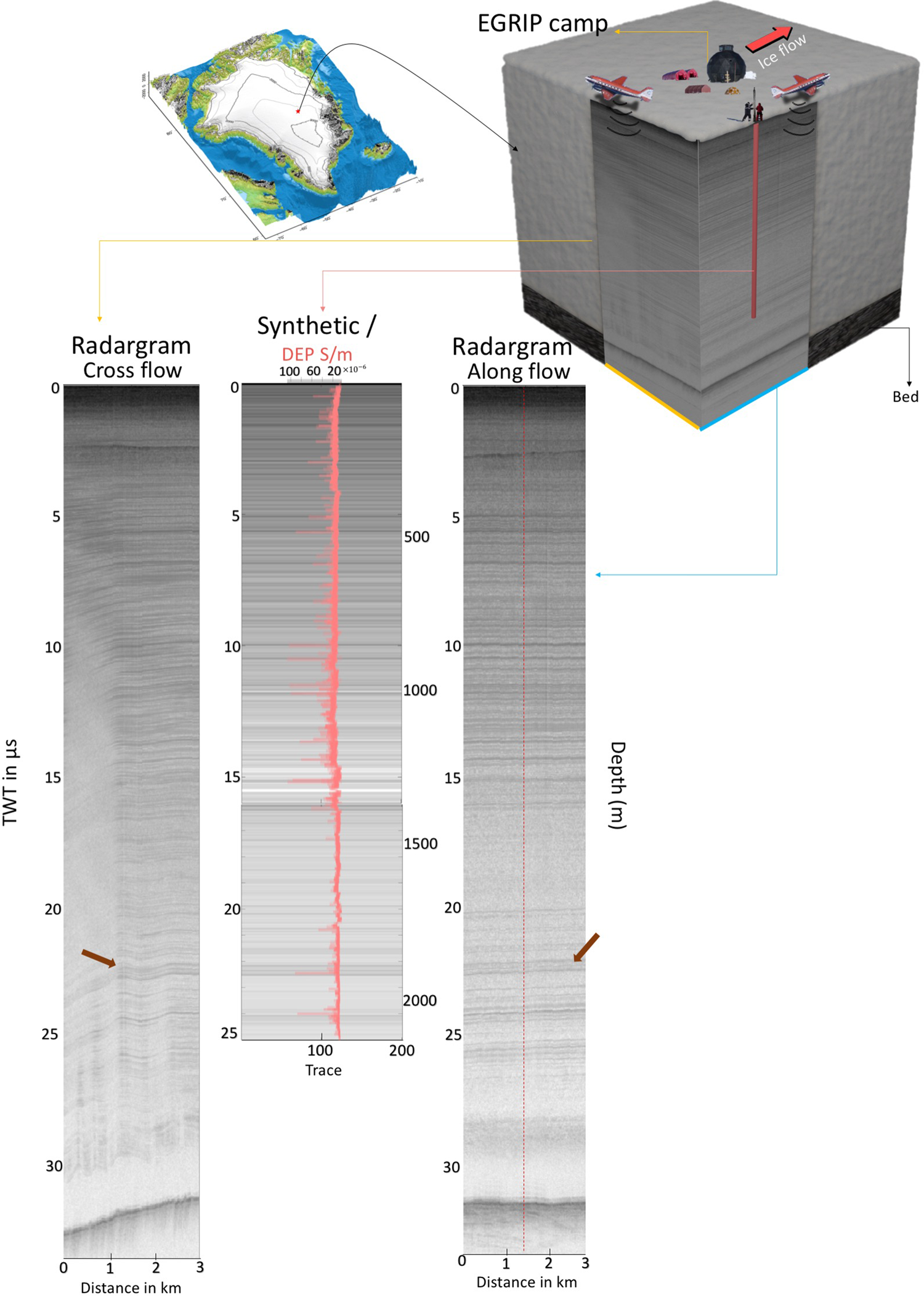
To underline the direct connection between ice-core dielectric properties and radar signals further, but also to illustrate the direction-dependent depth of IRHs in radargrams, Figure 4 shows a modelled radargram based on EGRIP DEP data, and two RES profiles oriented along and across-flow direction (see cartoon in Fig. 4). Conductivity changes can explain most of the IRHs at the EGRIP drill site. It also shows an effect of the flow velocity changes in the shear margins of NEGIS, which causes folding (Robert and others, Reference Robert, Anthony, David, Steven and David1993) (Fig. 4) in the profile oriented across ice-flow. The folding is apparent in the stratigraphy by strongly inclined reflections, which have a much larger spatial gradient than along-flow which results in weak signals (brown arrows in Fig. 4). In the case that only a single radar profile near a core site is available, such variations in the radar signatures (see RES cross-flow profile in Fig. 4), which depend on the direction of the profile, have to be considered when matching radar observations and ice-core data.
Previous studies (Dahl-Jensen and others, Reference Dahl-Jensen2013; Eichler and others, Reference Eichler, Weikusat and Kipfstuhl2013; Montagnat and others, Reference Montagnat2014; Li and others, Reference Li2018) showed that the NEEM core is a folded core with a strong change in the COF at 2200 m depth (Fig. 5). As mentioned above, we identify a strong reflection at ~ 22.2 μs i.e. around 1889 m depth that is only reproduced with a small signal in our synthetic result. The faint signals in the synthetic trace indicate that there is a small signal linked to the conductivity in the DEP data. The observed large peak at 22.2 μs in the RES data could indicate that the source of the IRH is not only due to a change in conductivity, as we observed it in the DEP data. At that depth, another possibility for the source of the IRH is the sudden change of COF. The change of eigenvalues and fabric images (c-axes) (Eichler and others, Reference Eichler, Weikusat and Kipfstuhl2013) correspond to this depth at 22.2 μs in Figure 5. Our interpretation is therefore similar to the one by Eisen and others (Reference Eisen, Hamann, Kipfstuhl, Steinhage and Wilhelms2007), who also indicated that a radar reflection at ~2040 m depth at the EDML drill site in Antarctica resulted from changes in crystal-orientation fabric.
At two ice-core sites, we have deep sections without any significant reflections: at NGRIP2 below 30 μs TWT, and at NEEM below 25 μs TWT. In Antarctica, the deepest part of the ice sheet is described as an echo-free zone (EFZ) (e.g. Fujita and others, Reference Fujita1999; Drews and others, Reference Drews2009; Winter and others, Reference Winter2017) which is characterized by a sudden drop of returned power in the RES data. A study by Drews and others (Reference Drews2009) shows disappearance of continuous IRHs in deeper sections of the Antarctic EDML drill site, related to changing physical properties. As the NEEM ice core has a continuous DEP record down to the bedrock (Dahl-Jensen and others, Reference Dahl-Jensen2013) we can conclude for the Greenland sites that the origin of these low-backscatter zones is rather related to low variability in dielectric properties and lower sensitivity of the radar system in use.
Possible across-flow concentrated fabric at EGRIP
We analysed the differences in the traveltime of unambiguously identifiable reflections in two perpendicular profiles near EGRIP, one along-flow, the other cross-flow. We translated these into the bulk anisotropy of permittivity (Table 4 in Appendix B ‘Anisotropy’), which is inherently related to the COF. Evidently, below a depth of 980 m down to our last matching IRH at 2041 m depth, the permittivity shows the strongest possible difference between cross and along flow. However, as also shown in Table 3, the relative error ($\sigma ( \varepsilon _\perp -\varepsilon _\parallel ) ) / ( \varepsilon _\perp -\varepsilon _\parallel )$ ranges between 30 and 70%, with an average of 56%. This error comes along with uncertainties in TWT determination and is too large to make strong quantitative conclusions about the type of fabric (e.g. horizontally transverse isotropic single maximum versus strongly aligned girdle), its exact orientation or its evolution with depth. Nevertheless, our analysis is robust enough to make two statements: first, the fabric shows a strong anisotropy in the horizontal plane, indicating at least a girdle fabric; second, given that the permittivity cross-flow is larger than the permittivity along flow, this implies that the c-axes are concentrated in the plane perpendicular to the flow direction. In a flow regime with uniaxial extension, a fabric with c-axes concentrated in the plane perpendicular to extension direction develops. Our interpretation of the RES-based analysis of anisotropy is in agreement with the finding observed in the EGRIP ice core (Westhoff and others, Reference Westhoff2021), who place the c-axes in the regional reference frame in a plane roughly northwest-southeast. Both results are supporting a fabric which is consistent with horizontal extension in flow direction at the EGRIP site. Methodologically, it is attractive to apply this approach on a routine basis to those regions where several crossing radar profiles are available in order to determine the horizontal anisotropy of the bulk fabric. Increasing the number of crossover points in such an analysis, as for instance available for the EGRIP-NOR-2018 survey, would also reduce the overall influence of the relatively large uncertainty from deducing horizontal anisotropy from single IRHs only. As ice-stream dynamics induces particular fabric patterns, the application of our approach described here as well as other approaches (e.g. Young and others, Reference Young2021) have the potential to eventually a more consistent way to characterize ice stream properties on a regional scale and not only at point locations.
Age stratigraphy
By linking the dated events from DEP records at the locations of three deep ice cores to reflections in airborne RES data, we are able to provide a more accurate dating of the radar IRHs, which can then be extended along the radar lines over large parts of northern Greenland (e.g. MacGregor and others, Reference MacGregor2015). Using our forward modelling approach, the depth uncertainties of the IRHs are reduced compared to the common TWT-to-depth conversion with a constant electromagnetic wave speed approach. With the forward DEP modelling approach, the depth uncertainties are related to the DEP measurements and the width of the reflection-causing conductivity peaks (Winter and others, Reference Winter, Steinhage, Creyts, Kleiner and Eisen2019). Our age stratigraphy with a direct connection of different deep ice cores can be used to better understand internal processes (i.e. ice deformation) in the Greenland Ice Sheet. It could also provide an improved assessment of age accuracy in northern Greenland, as the one provided by MacGregor and others (Reference MacGregor2015) for the Greenland Ice Sheet.
Conclusions
We have characterized the origin of the IRHs inside the Greenland Ice Sheet by radar forward modelling. In order to understand physical processes that cause the IRH and identify ages for the reflectors causing the layers, we rely on the airborne radar measurements and modelling of synthetic radar traces that were fed by conductivity and permittivity data from EGRIP, NEEM and NGRIP2 ice cores in Greenland. Our results show excellent agreement for most of the IRHs between the synthetic results and the RES measurements. From the comparison between the measured and modelled traces, we conclude that conductivity peaks are responsible for most radar IRHs. Overall, the modelling results demonstrate that the internal reflections of the ice sheet are due mostly to conductivity changes. In some cases, however, conductivity plays only a minor role and the dominant reflection mechanisms seem to be anisotropic backscatter at interfaces where the bulk fabric changes. IRHs in the observed radargrams have been dated by means of the presented sensitivity studies with the DEP record using the GICC05 time scale. For EGRIP our comparison of along and cross-flow wave propagation speeds suggests a concentration of the c-axes in a girdle perpendicular to the flow direction (below 980 meters). Based on this analysis, we are able to orient the observed fabric in the ice core in the absolute reference frame of the ice sheet and support the discussed flow regime of uniaxial extension. This approach could be extended to map the horizontal anisotropy in larger regions where numerous radar lines crossovers are available. Given that our thorough understanding of complex ice-stream dynamics is a key requirement to improve paleo-reconstruction and prognoses of future ice-stream behaviour, especially for sea-level projections. Unfortunately, the current horizontal anisotropy does not represent into ice-sheet models, while anisotropic ice can enhance the speed of ice flow (Glen, Reference Glen1958). We recommend extending our approach to more thoroughly map horizontal anisotropy in regions where numerous crossing of radar lines are available and plan future surveys accordingly.
Data availability
-
Specific conductivity measured with the dielectric profiling (DEP) technique on the EGRIP ice core, 1383.84-2122.445 m depth (https://doi.pangaea.de/10.1594/PANGAEA.922285).
-
Permittivity measured with the dielectric profiling (DEP) technique on the EGRIP ice core, 1383.84-2122.445 m depth (https://doi.pangaea.de/10.1594/PANGAEA.922299).
-
Specific conductivity measured with the dielectric profiling (DEP) technique on the NEEM ice core (1493.297-1757.310 m depth) (https://doi.pangaea.de/10.1594/PANGAEA.922303).
-
Permittivity measured with the dielectric profiling (DEP) technique on the NEEM ice core (1493.297-1757.310 m depth) (https://doi.pangaea.de/10.1594/PANGAEA.922305).
-
Specific conductivity measured with the dielectric profiling (DEP) technique on the NGRIP2 ice core (down to 1298.555 m depth) (https://doi.pangaea.de/10.1594/PANGAEA.922306).
-
Permittivity measured with the dielectric profiling (DEP) technique on the NGRIP2 ice core (down to 1298.555 m depth) (https://doi.pangaea.de/10.1594/PANGAEA.922308).
-
AWI ultra-wideband (UWB) airborne radar data around the EastGRIP drill site at the onset region of the Northeast Greenland Ice Stream (https://doi.pangaea.de/10.1594/PANGAEA.932334).
Acknowledgements
We thank three anonymous reviewers for fruitful comments that improved the paper a lot. EGRIP is directed and organized by the Centre for Ice and Climate at the Niels Bohr Institute, University of Copenhagen. It is supported by funding agencies and institutions in Denmark (A. P. Møller Foundation, University of Copenhagen), USA (US National Science Foundation, Office of Polar Programs), Germany (Alfred Wegener Institute, Helmholtz Centre for Polar and Marine Research), Japan (National Institute of Polar Research and Arctic Challenge for Sustainability), Norway (University of Bergen and Bergen Research Foundation), Switzerland (Swiss National Science Foundation), France (French Polar Institute Paul-Emile Victor, Institute for Geosciences and Environmental research) and China (Chinese Academy of Sciences and Beijing Normal University). We acknowledge the use of data from CReSIS generated with support from the University of Kansas, NASA Operation IceBridge grant NNX16AH54G, NSF grants ACI-1443054, OPP-1739003, and IIS-1838230, Lilly Endowment Incorporated, and Indiana METACyt Initiative. Dorthe Dahl-Jensen acknowledges Villum Investigator IceFlow (grant nr16572). We thank Sepp Kipfstuhl, Nanna B. Karlsson, Sergio Henrique Faria, Vasileios Gkinis and Helle Astrid Kjær for helping to measure DEP data during 2017 and 2018 seasons in EGRIP camp. We thank Eliza Cook, Tobias Erhardt and all people involved in ice-core processing, drilling and logistics in the field. We thank Tobias Binder, who helped with the radar measurements and the crew of the aircraft Polar6 and system engineer Lukas Kandora during the AWI flight campaign 2018. We thank Sepp Kipfstuhl for assistance with the NGRIP2 DEP data.
Author contributions
SM wrote the manuscript and conducted the main part of analysis; figures were created by SM; synthetic radar modelling was done by SM using the emice model implemented by OE; DEP measurements in the field were done by SM; DEP data processing was done by SM and FW; selection and compilation of radar data sets were done by SM, SF; AWI UWB radar processing was done by SF, DS; AWI (Polar6 aircraft, 2018) measurements in the field were done by DJ, JP; EGRIP anisotropy analysis was done by SM, FW; NEEM COF data processing was done by IW and JE; data interpretations were done by SM, OE, FW; all authors contributed to improving the writing and discussing of paper.
Appendix A.
Details on the modelling of synthetic radar traces
In order to convert the depth of DEP data to the two-way travel time (TWT) domain of the RES data, we need to determine the electromagnetic wave speed in firn and ice c z with the speed of light in a vacuum c 0 and the real component ɛ′ of the complex relative dielectric permittivity, $\varepsilon ^\ast$ ,
,

In these equations, ɛ″ is the imaginary component of the complex relative dielectric permittivity, σ is the electric conductivity, ɛ 0 the dielectric permittivity of the vacuum and ω the circular frequency.
Firn in the uppermost fraction of the core is a two-phase system, being composed of ice and air. Air has a relative permittivity of 1 and basically zero conductivity (free-air conductance, as determined from an empty DEP device (Mojtabavi and others, Reference Mojtabavi2020)), while the ice phase of pure glacier ice exhibits the relative permittivity ɛ ice′ and the conductivity σ ice, which is determined by the chemical impurity load and the temperature of the ice. The complex relative dielectric permittivity $\varepsilon ^\ast$ of the mixture further depends on the volume fraction of the ice phase, here being expressed as the fraction of firn density ρ and pure ice density ρ ice. The dielectric property of the firn is well described by the density and conductivity mixed permittivity (DECOMP) equation (Wilhelms, Reference Wilhelms2005):

Thus, we determine density and conductivity, which are frequency independent, from the DEP measurements and calculate the input to our model at the central frequency of the radar system by means of the DECOMP formula (Eisen and others, Reference Eisen, Wilhelms, Steinhage and Schwander2006).
The imaginary and real parts of the complex dielectric permittivity were measured directly in the field with a DEP bench at a frequency of 250 kHz for all ice cores. The ‘emice’ model basically translates their variability with depths into reflection signatures of the impulse response of the subsurface. However, general amplitude decay with depth is not reproduced by the model as it operates in 1D only.
We used 0.02 m as model depth resolution and 0.02 ns for the time increment. These values are based on the stability of the numerical calculations (Eisen and others, Reference Eisen, Wilhelms, Steinhage and Schwander2006). The maximum depth varies for each ice core. We used a physical model domain equivalent to 35 and 36 μs TWT for the NEEM and NGRIP2 ice cores, respectively, to cover reflection in our model domain. The final logging depth for EGRIP is 2122.445 m which was drilled in field season 2019, i.e. not yet reaching bedrock. Therefore, we used 30 μs TWT to cover reflection in our synthetic model domain for the EGRIP ice core. The time ranges and the upper boundary of the model were selected sufficiently large to only cover reflections from the model boundaries based on the ice core depths, but to avoid artificial reflections from the model boundaries. Radar measurements suggest the ice thickness likely exceeds 2550 m (Vallelonga and others, Reference Vallelonga2014). Due to the integration over kilometres, the average dielectric permittivity for a depth interval may be determined even more precisely from the radar sounding than the estimated 1–2% error of the DEP measurement (Wilhelms and others, Reference Wilhelms, Kipfstuhl, Miller, Heinloth and Firestone1998; Wilhelms, Reference Wilhelms2005; Mojtabavi and others, Reference Mojtabavi2020). For sections below 100 m depth, we compared the synthetic traces calculated with varied real part of permittivity (3.15, 3.16, 3.17, 3.18 and 3.19) with observational radar traces TWT to find the best electromagnetic wave speed c z which results in the best match or synthetic and observed radar reflections, where c z and ɛ′ are closely related through Eqn (A.1). The real permittivity of the DEP record varies within the estimated 1–2% error. Apart from this methodological limitation of DEP, the permittivity offset along the symmetry axis of an ice crystal and perpendicular to it is close to 1% as well (Fujita and others, Reference Fujita, Mae and Matsuoka1993). Site-dependent evolution of the crystal orientation fabric (COF) together with the lacking knowledge about the orientation of the cores (Westhoff and others, Reference Westhoff2021), may also explain the observed variation on the permittivity records’ real part. The correspondence of modelled and measured radar-traces is improved when replacing the measured dielectric permittivity's real part with a fixed average value. Therefore, an average value of permittivity can produce the reflections caused by variation in conductivity at the accurate TWT and avoids interference from reflections due to noise in the real part's record. Winter and others (Reference Winter2017) found a best match for a dielectric permittivity constant of 3.17 for the modelling based on the EDC ice core in Antarctica. In this study, we determined a value of 3.15 value for all ice cores which represents the best correspondence between model and measured traces for the glacial ice sections below 100 m.
Appendix B.
Anisotropy
The recorded depth of the DEP conductivity peaks s, the TWT $t_\parallel$ along flow, the TWT t ⊥ cross-flow, the permittivity $\varepsilon '_\parallel$
 in polarization direction along flow, the permittivity $\varepsilon '_\perp$
 in polarization direction cross-flow, the difference $\varepsilon '_\perp -\varepsilon '_\parallel$
 and the average permittivity $( {\varepsilon '_\perp + \varepsilon '_\parallel }) /{2}$
 , the errors of the calculated permittivities $\sigma ( \varepsilon '_{\parallel })$
 and $\sigma(\varepsilon '_\perp)$
 and the error of the difference$.$


 Open access