


Impact Statement
Digital twins are increasingly discussed to optimize urban energy use and agriculture, and we suggest they are particularly suited to bespoke environments, for which conventional “one size fits all” models cannot cater to their changing operational conditions. We present the development of a digital twin for an urban-integrated hydroponic farm, situated in repurposed WW2 air raid shelters in London. We show how a digital twin can faithfully represent the reality of the environment through real-time streams of data, making it a useful representation for an operator of the farm. Digital twins are not easy to develop in unique environments, and we present the challenges and opportunities through the three crucial elements of a digital twin. (a) Data Creation: an extensive monitoring system that combines wireless sensors with manual data records to create a virtual representation of the farm through data. (b) Data Analysis: key influencing variables on energy use and crop yield can be identified by analyzing the relationships between the broad data collected. (c) Data Modeling: the digital twin is an opportunity to apply site-specific modeling to forecast potential future operational scenarios, and provide feedback on the influence of recent events on farm environment.
1. Introduction
As wireless sensor technology, large cloud databases, and computer processing power become more available (Qi et al., Reference Qi, Tao, Hu, Anwer, Liu, Wei, Wang and Nee2019), data-centric solutions in the form of digital twins are attractive to improve performance and efficiencies of built environments both of innovative and traditional enterprises alike (Kaewunruen et al., Reference Kaewunruen, Rungskunroch and Welsh2018; Ruohomaki et al., Reference Ruohomaki, Airaksinen, Huuska, Kesaniemi, Martikka and Suomisto2018). As we will demonstrate in this paper, the benefits of a digital twin are especially pronounced in built environments that are bespoke and where standard asset management and control systems provide limited utility. Although digital twins are still in the process of being defined by scholars (Jones et al., Reference Jones, Snider, Nassehi, Yon and Hicks2020), they are broadly understood to be virtual representations of an existing object or process, including continuously monitored data that provides feedback for optimal management of the twinned object or process.
This paper presents the development of a digital twin of a unique hydroponic underground farm in London. Growing 12 times more per unit area than traditional greenhouse farming in the UK, the farm also consumes four times more energy per unit area (Milà Canals et al., Reference Milà Canals, Muñoz, Hospido, Plassmann, McLaren, Hounsome, Milà, Ivan, Almudena, Katharina and Sarah McLaren2008; The Carbon Trust, 2012). Key to the ongoing operational success of this farm and similar enterprises is finding ways to minimize the energy use while maximizing crop growth by maintaining optimal growing conditions.
As such, the farm belongs to the broad class of Controlled Environment Agriculture (CEA), where indoor environments are carefully controlled to maximize crop growth by using artificial lighting and smart heating, ventilation, and air conditioning (HVAC) systems (van Straten and Henten, Reference van Straten and Henten2010). There is a vast literature on monitoring and optimizing CEA environments and recently digital twins have started to be implemented in smart farming to identify pests and diseases, animal feed availability, or track machinery in fields through telemetry (Verdouw and Kruize, Reference Verdouw and Kruize2017). In Japan, the use of the “SAIBAIX” dashboard is starting to be used in smart plant factories, where real-time sensor information can keep farmers informed about the current farm productivity and resource use efficiency (Sakaguchi, Reference Sakaguchi2018). However, using the data for analysis and modeling is error prone owing to quality of data, and the authors conceded further work was needed to make robust data-learning models. The few examples of digital twins that exist in CEA environments “mostly focus on basic monitoring capabilities or they virtualize objects at a high granularity level” (Verdouw and Kruize, Reference Verdouw and Kruize2017). For example, Alves et al. (Reference Alves, Souza, Maia, Tran, Kamienski, Soininen, Aquino and Lima2019) presented their initial development of a digital twin for smart farming, where they could visualize data of a soil probe on a dashboard but were not at the stage of a fully operating digital twin with feedback and analytics. Hemming et al. (Reference Hemming, De Zwart, Elings, Righini and Petropoulou2019) presented the results of a competition on the use of Artificial Intelligence (AI) to optimize the controls of a greenhouse by linking sensor data to operable controls. They showed that artificial neural networks have great potential to optimize crop growth, but the trials were conducted on an ideal testbed greenhouse.
The farm which is the subject of this paper is unique because unlike traditional CEA, it is 33 m underground in tunnels where the environment cannot be precisely controlled. Whilst the ground surrounding the tunnels does provide constant boundary conditions (unlike standard CEA, which are subjected to fluctuations of outdoor weather), the limited access to ventilation and constrained access for farm operations poses challenges. Furthermore, the farm is entirely reliant on LED (Light Emitting Diode) lights to activate the photosynthesis process for plant growth. Finally, the practical challenges of setting up a monitoring network in the continuously changing environment of urban integrated or innovative farms are poorly reported, but a crucial element to the success of such endeavors, especially as cities are demonstrating an increased interest in urban agriculture.
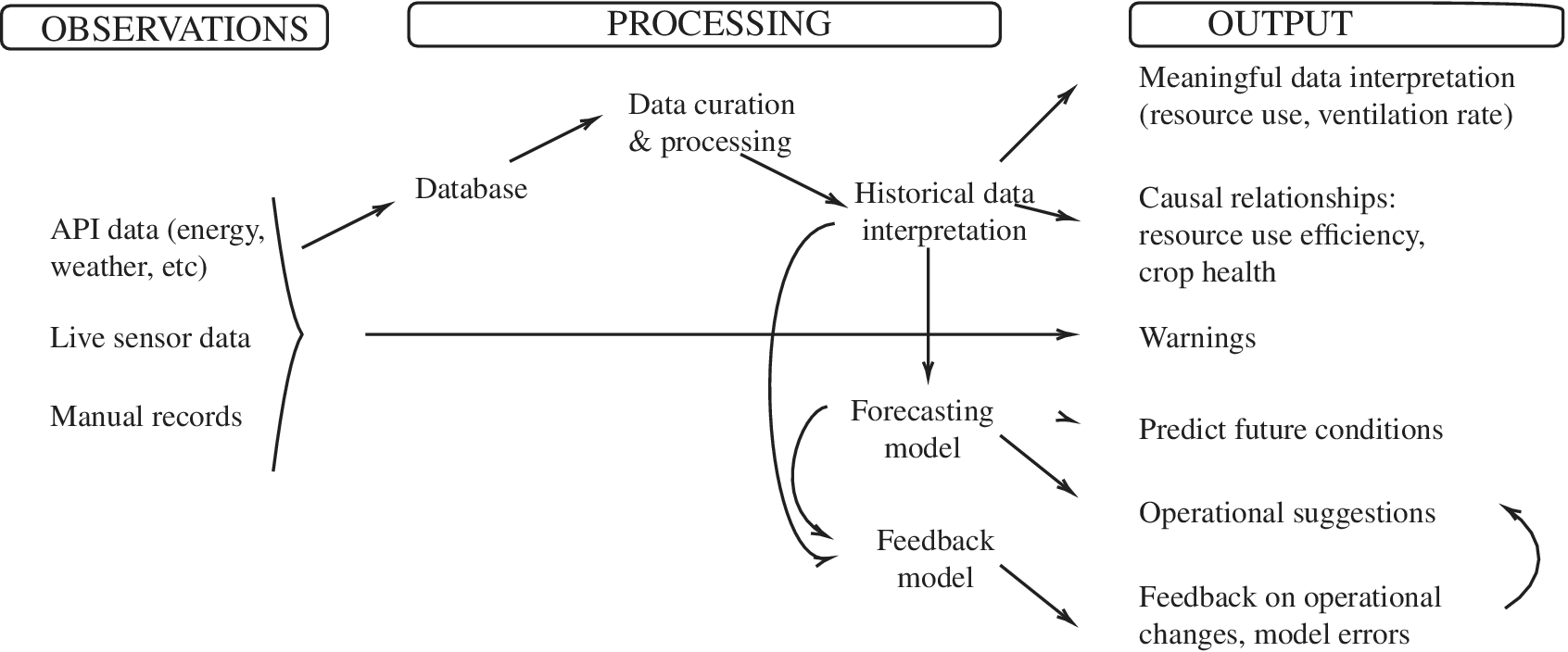
The overarching objective of this paper is a digital twin of the underground farm that faithfully represents the reality of the environment through real-time streams of data, making it a useful representation for an operator of the farm. This includes three crucial elements: (a) Data Creation: An extensive and robust monitoring system that tracks the observable environmental conditions in the underground farm. This is supported by data curation that ensures quality and tractability of data. (b) Data Analysis: Using observable data in conjunction with information reported by farm operators to identify key influencing variables of the farm environment and thereby on crop yield. (c) Data Modeling: We investigate techniques most suitable for identifying critical trends and changes, forecast potential future operational scenarios, and provide feedback on the influence of recent events on farm environment.
Despite the upcoming body of literature on digital twins, examples of digital twins that successfully and seamlessly integrate these elements in a fully operational and complex environment are rare, and thus this paper fills this important gap in academic literature. As we will show in Section 6, a second novel feature of this paper is the forecasting model that is easily implementable with as little as temperature and energy meter readings, and flexible to the addition of more data as it becomes available.
The structure of the paper follows the representation of the digital twin in Figure 1. We first present the monitoring process and the key data challenges of monitoring in a continuously operated environment. In Sections 4 and 5, we present the data analysis that includes: (a) the influence of the farm environment on crop growth, (b) the influence of operable controls on the environment, and (c) the influence of manual changes on the operational controls. Within the limitations of the data, this exercise identifies the variables which are crucial to track and forecast. We then present the data model, which is essentially a forecasting model that predicts extreme temperatures and provides feedback on operational changes that can reduce energy use and control the farm environment more effectively. We conclude with a discussion on further development of this digital twin.
The three integrated stages of a digital twin applied to GU.
2. Brief Overview of the Underground Farm
Growing UndergroundFootnote 1 (GU) is an unheated hydroponic farm producing microgreens. It is situated in derelict tunnels designed as a WW2 air raid shelter in the 1940s, 33 m below ground. The tunnels had not been used since they last housed the Windrush generation of migrants in the 60s, until the farm opened in December 2015. The farm initially catered to hotels and restaurants and has expanded to become a supplier of large UK food retailers such as M&S and Ocado. The main crops are peashoots, basil, coriander, parsley, salad rocket, pink radish, and mustard plants.
The site consists of two parallel tunnels, running on two levels and spanning approximately 400 m (Figure 2). Currently, only half the upper tunnel is used for growing crops, in an area of 528 m2 and is projected for major extensions from August to December 2020.
Map of the tunnels onto London. In red, the currently occupied tunnels 1–3. In blue, the tunnels 5–8 are planned for the extension. The current farm is in tunnel 3, as shown in the picture “Farm.” The two entrances to the farm, CP and Clapham Common (CC), are also shown with pictures and linked to the location on the map.
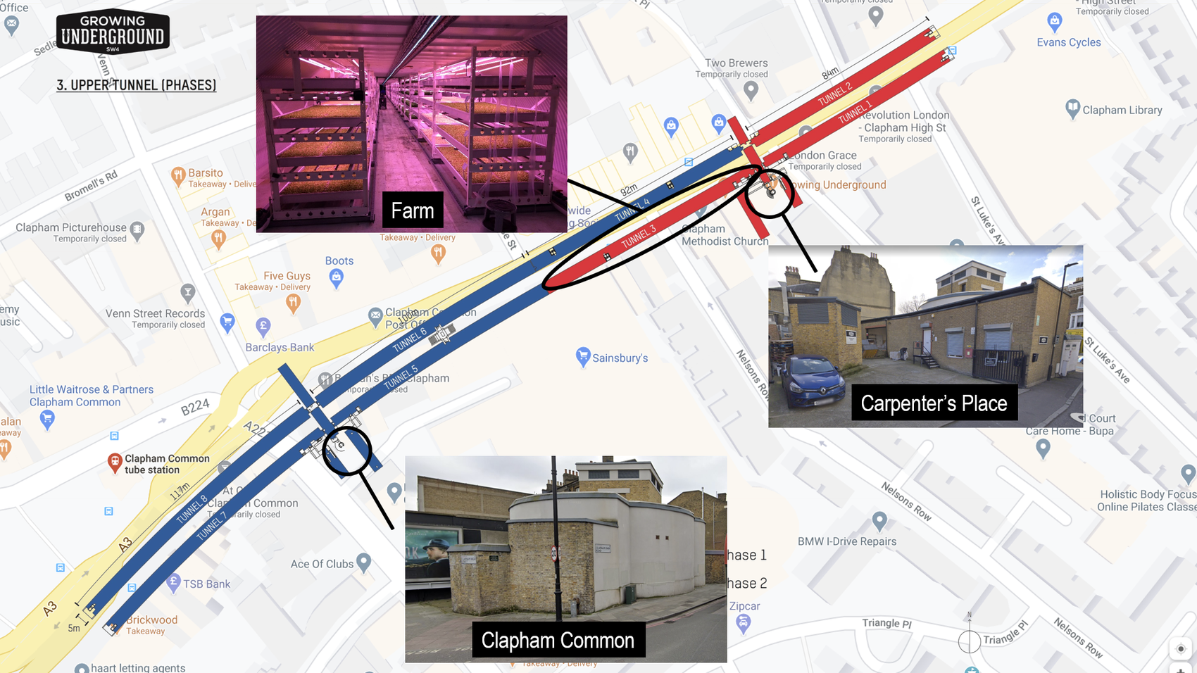
The current farm is located in the upper tunnel of Tunnel 1 (circled tunnel in Figure 2), near the Carpenter’s Place (CP) entrance. The lower tunnel contains 20 irrigation tanks of 1 m3 each, 10 with fresh water, and 10 with recycled water. The fresh water tanks irrigate the farm in the upper tunnel twice a day using an ebb and flow mechanism which floods the trays for 15 min. The water that is not absorbed by the mats on the benches gets recirculated to the recycled water tanks. The water that circulated through the zones containing allergens is removed due to the risk of contamination.
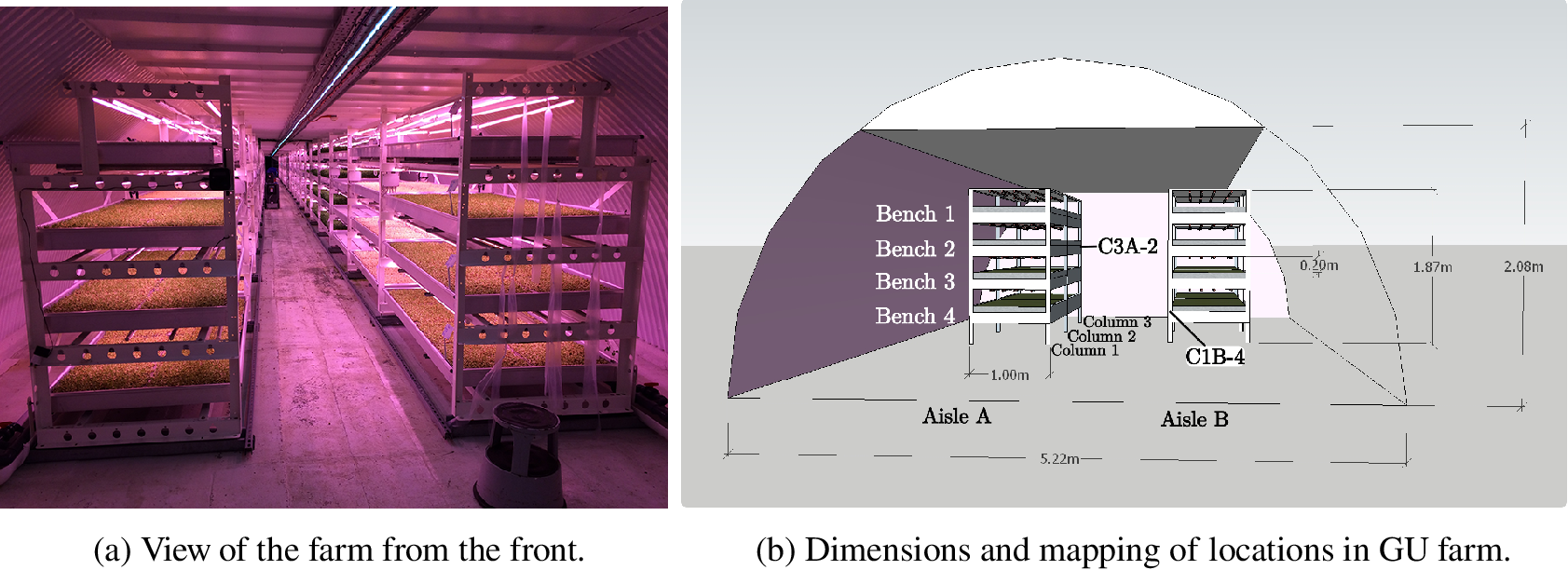
The farm itself consists of two areas hereafter called the “original farm” installed in January 2016 and the “extended farm,” installed during January 2018, and is organized in terms of aisles, columns, stacks, and benches (see Figure 3). This brings the total farm area to 528 m2, with 460 m2 in the original farm, and 68 m2 in the extended farm. The tunnel footprint itself is 519 m2, making an area efficiency ratio of 1.03, which is very high for an indoor farm including passage space. Despite the tunnel only having a ceiling height of 2.08 m, each stack is 1.87 m high and houses four benches, spanning 2 m in width, with a surface area of 2 m2. The stacks are aligned in two parallel aisles, known as aisle A and aisle B. There are 24 columns surrounding 23 stacks in each aisle in the original farm, and 10 columns with nine stacks per aisle in the extended farm. The relative locations in the farm will henceforth be denominated as such: C3A-2 will refer to Column 3, aisle A, bench 2, as marked in the diagram in Figure 3.
Photograph and 3D drawing of the front of the farm.
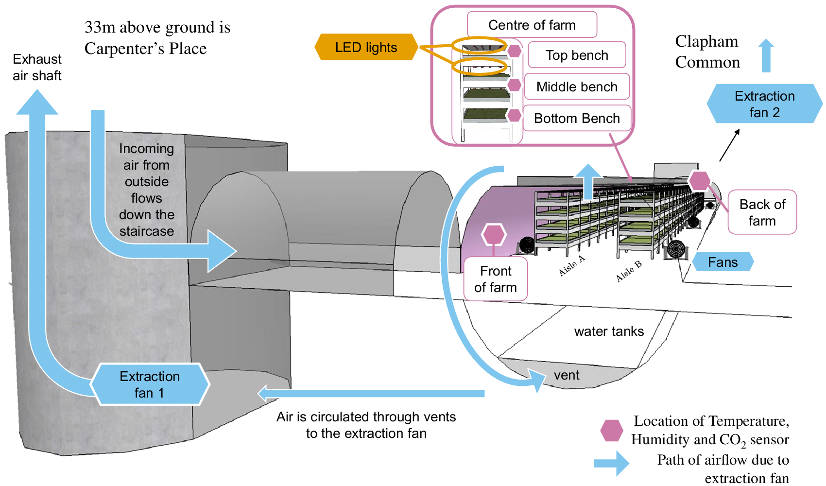
The entrance to the tunnel is in CP, depicted in Figure 2. A spiral staircase surrounds the lift that brings the staff down to the farm, but which is also the main ventilation axis. Indeed, the air is drawn in through the staircase and circulated through the tunnels with vents in the ceiling of the upper tunnels, and in the floor of the lower tunnels. This air is drawn by a 30 kW extraction fan located in the lower tunnel. The extraction fan unit consists of two fans which alternate to prevent overheating. The air is drawn out through a parallel vertical shaft to the staircase, and the vents are visible opposite the CP entrance in Figure 2. An identical fan is located below CC (also illustrated in Figure 2), which draws the air down the CC staircase, and is designed to circulate the air through tunnels 5–8, and extracts back up a ventilation shaft. Each fan has its designated tunnels (CP is for tunnels 1–4 and CC is for tunnels 5–8), but the effect of the fan at CC is felt in the farm as well because the tunnels 4–8 are currently completely empty.
The farm tends to be occupied in the mornings (6–8 am) to harvest the fresh produce, and in the evenings (3–4 pm), to exchange the crops. GU also regularly organizes tours of the farm where groups of 4–15 visit for approximately 1 hr at varying times of the day. The farm is less busy at weekends.
By virtue of being underground, the farm is artificially lit, giving the operators more control over when to start the photoperiod than in conventional greenhouses. Each bench in the farm is lit by four LED growing lights, of length 1.5 m, named AP673L from the manufacturer Valoya, with a photosynthetically active radiation intensity of 1.9 μmol W−1 s−1 (Valoya, Reference Valoya2016). In the original farm, the lights are AP673L 30 W and AP673L 40 W in the extended farm. While the lighting schedule has varied across the monitoring period between 14 and 18 hr, the target duration of the photoperiod is 18 hr with a night period of 6 hr when the lights are turned off. As energy is cheaper at night, the target farm daytime is between 5 pm and 11 am. If on for 18 hr, this corresponds to a daily light integral of 9.8 and 13 mol m−2 day, which is within the target range of environmental PAR integral defined for lettuce by Ferentinos et al. (Reference Ferentinos, Albright and Ramani2000) of 11–17 mol m−2 day.
3. The Monitoring Network
A prerequisite of digital twinning is an appropriate monitoring network that provides relevant information exchange between the system and its virtual counterpart. Indeed, a robust and efficient monitoring network is a key element that drives a digital twin and sustaining it through the life cycle of a system is often challenging. Sensors that constitute the monitoring network are known for their limitations with respect to low battery power, limited computational capability, and small memory (Aqeel-ur-Rehman et al., Reference Aqeel-ur-Rehman, Abbasi, Islam and Shaikh2014). In addition, underground tunnels present issues of communication across a fragile wireless network. Finally, human factors and operational constraints can pose limitations with respect to appropriately locating sensors and communication lines.
Consequently, a range of sensors were trialed to ensure that the information from the monitoring network is accurate, relevant, and continuous. This in principle constitutes the design of a wireless sensor network (WSN) which sends data in real time to a server. The WSN consists of 25 sensors, monitoring a total of 89 variables, which transmit data to eight Raspberry Pi (Raspi) loggers. These loggers in turn transfer the data to servers in the Cambridge University Engineering Department (server) over WiFi. The loggers also store the data on SD cards when the wireless service goes down. Each data logger (Raspi 1–8) is connected to sensors with a unique identifier, categorized as “Sensor Name” in Figure 4. The five environmental variables that are continuously monitored are temperature, relative humidity (RH), CO2 concentration, air velocity, and light levels. Some of these, such as temperature are monitored by several sensors, linked to different data loggers (e.g., Raspi 1, 6, 7, and TinyTag). The reader is referred to Jans-Singh et al. (Reference Jans-Singh, Fidler, Ward and Choudhary2019) for detailed information about each type of monitored variable.
Diagram of the data collection and storage network, showing the automatic wireless (dotted lines), automatic wired (dashed) data transfers, and data which need manual data collection (full line). See text for details.
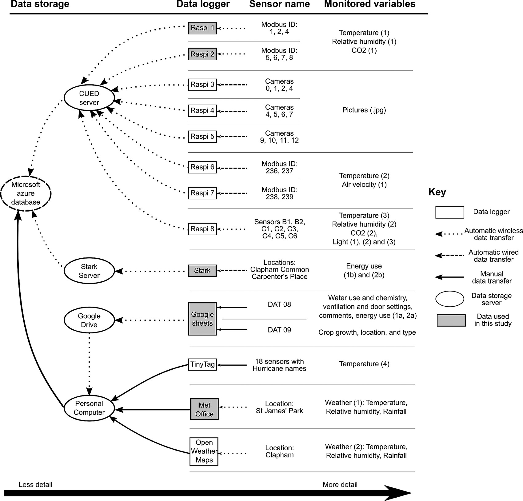
At the same time, information that can be feasibly obtained from the wireless network is only partial. Therefore a system was created for manually logging operational conditions such as ventilation settings or lighting schedules (Jans-Singh et al., Reference Jans-Singh, Fidler, Ward and Choudhary2019). The observations of the farm thus fall into two categories: the structured data, consisting of the WSN, and continuous data from energy meter readings from Stark and weather from the MetOffice; and “unstructured data,” which are manually recorded observations.
Data from these different sources are stored in a Microsoft Azure database, as summarized in Figure 4. To the left of the diagram are the servers storing the data, and to the right are the monitored variables recorded by each data logger–sensor combinations. The line type of arrows indicates the type of data transmission (wireless or wired, manual, or automatic). A web platform is under development to visualize in real-time the data acquisition and historical data. Both the raw real-time data and curated historical data are used for data analytics and data modeling.
The five sets of data presented in this paper are marked in Figure 4 by greyed boxes. The data were chosen because they had the longest data range available and because they represented a wide range of data collection methods and variables. The period over which records now exist is shown in Figure 5 up to summer 2016, with hourly weather conditions data accessed for St James’ Park from the UK Met Office.
Data availability for monitored variables used in this study.

The sensors linked to the Raspi 1 and 2 data loggers are wireless Advanticsys IAQM-THCO2 motes (Advanticsys, 2017), which log temperature, humidity, and CO2. Five of the seven sensors were installed in the farm, and their locations are marked in Figure 6 with pink hexagons. For this paper, we focus on temperature and humidity readings as the CO2 data are unreliable due to sensor drift (Jans-Singh et al., Reference Jans-Singh, Fidler, Ward and Choudhary2019). The data are almost complete since September 2016 (Figure 7).
Location of sensors in GU. The side view of a typical bench is indicated for the centre of the farm, showing how four LED lights span the length of each bench. The blue arrows indicate the air circulation throughout the farm caused by EF1 at CP.
Missing sensor data by location by hour over monitoring period used in this study. Left: black lines signify a missing data point for the hour on the x-axis. Right: percentage summary of missing points for the given sensor.

Energy use is recorded at half-hourly intervals using 2 meters located at the two ends of the tunnel, named CP and CC (Figure 2), and is accessed from the Stark server (Stark ID, Reference Stark2020). CP powers one extraction fan (called extraction fan 1) of 30 kW, and the 1024 LED lights in the farm of 30 W each. The energy signal thus primarily represents these two objects (fan 1 and lights), but also includes energy used for the office, package and processing, propagation, refrigeration, and lift. The reading at CC only measures the energy use of extraction fan 2 (fan 2, which is identical in specification to fan 1). The data for meter 1 became available from July 28, 2017, and meter 2 from January 26, 2018 (Figure 5).
Since it was not possible to automatically log crop data and individual actions in the farm, we assembled, together with GU, a set of manually recorded variables. Although the lights have an automated control board with two settings (on/off), the extraction fan has a manual control dial. The setting on the manual dial represents the ventilation rate of the extraction fan. The operators do not know to what extent they are modifying their energy use when changing the dial setting. The farm operators were instructed to record the ventilation setting whenever it is changed on a Google Spreadsheet (DAT 08 in Figure 4). This was done daily since January 26, 2017. Further manually recorded data include comments from the farm operators, such as records of whether doors were open or shut, addition of new fans, or moving any sensor from its original location.
Crop growth is recorded since March 2016, by crop type, mass, and area harvested. The location of each crop is tracked since March 2017 for each bench and column, according to the layout illustrated in Figure 3. These data are manually recorded by farmers processing the crop (DAT 09 in Figure 4), so in the midst of operations, it is prone to human error. Nonetheless, such data can give an indication of how environmental conditions influence crop growth.
In order to have a complete dataset which can be used for the development of the digital twin, any missing data must be regularly imputed. While linear interpolation suffices for the relatively small data gaps in some observations (e.g., the energy meter readings and Met Office weather data), the sensor data measuring temperature and humidity in the farm needed a more detailed imputation procedure. The prevalence of missing points for the five sensors of interest is illustrated in Figure 7. The data are missing at random and in blocks, indicating that missing data were more likely linked to general sensor failure due to unplugging, loss of internet connection, connectivity with the data logger, and not due to individual sensors on the monitors. The sensor locations with least missing values are connected to the same data logger, at the “Top bench” and “Front of the farm” (Figure 6) with around 8% missing data over the 907 days considered in this study, while the sensor with most missing values was located at the “Back of the farm.”
Sensor data were analyzed from September 2016 to February 2019, when there is almost always data from at least one sensor. The missing temperature measurements are imputed using a random forest algorithm with neighboring sensor data, outside weather conditions, and the hour of day, with 100 trees. More normally distributed, the humidity missing data are imputed using normal multivariate regression using neighboring humidity sensor values and external humidity, without including the hour of day. Both were performed with the mice package.
4. Data Analysis of Environmental Conditions
When given enough nutrients in a hydroponic system, crop growth is limited by three environmental factors: temperature, visible radiation, and CO2 levels (Blackman, Reference Blackman1905). As the farm is artificially lit for 18 hr a day, and the CO2 levels are roughly constant around 400 ppm due to ventilation, temperature is likely the most significant limiting factor for crop growth. Humidity is also a concern as levels over 70% can affect yields due to lower leaf resistance to pathogens (Stine et al., Reference Stine, Song, Choi and Gerba2005), but higher humidity can speed up the production of crops with a higher water content in shorter period of time (Tibbitts and Bottenberg, Reference Tibbitts and Bottenberg1976). This is expected to be a secondary factor as humidity in the farm is managed well with dehumidifiers.
Crop performance is assessed for nine of the most grown crops in the farm. Crop growth refers to the yield divided by the number of days the crop was in the farm. Crop performance is calculated as crop growth divided by its average crop growth. Thus a crop performance of 1.05 suggests that the crop grew 5% better than its average performance.
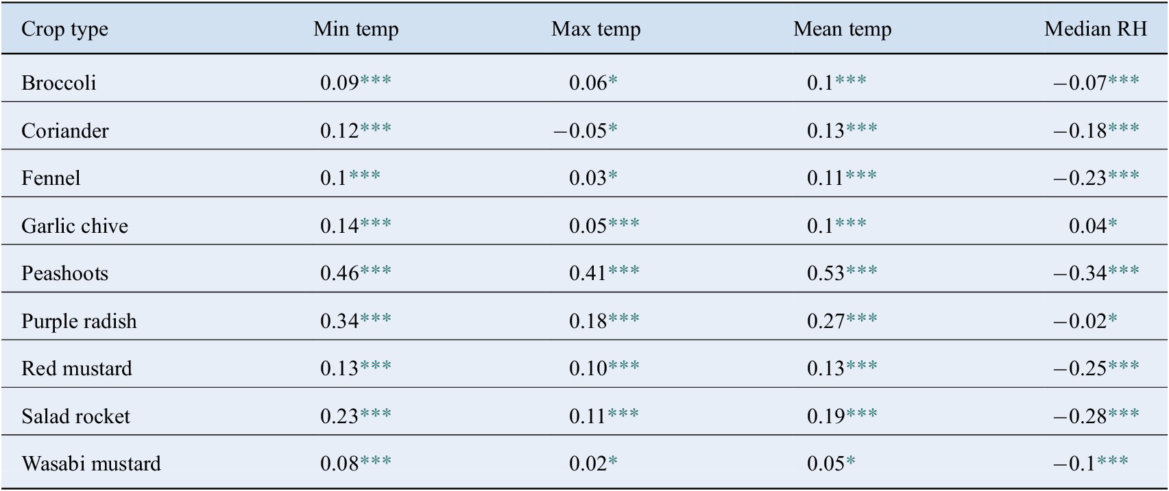
The correlation table (Table 1) shows the relationship between each crop’s performance and the minimum, maximum, and mean temperature during the crop’s time in the farm, and the median RH value. The correlation ( $ r $) and p-values ( $ p $) indicate the strength of the relationship between temperature and RH with crop growth. A high p-value ( $ p>.05 $, denoted by * in Table 1) signifies that there is not enough data to establish a strong relationship. High correlations with low p-values ( $ p<.05 $) indicate that there is significant evidence that crops grow better if temperature or humidity are increased/decreased. According to Table 1, most crops have a significant relationship with the mean and minimum temperature observed, and the median RH while they were in the farm. However, this relationship is stronger for some crops than others. For example, peashoots have high correlation and significant p-value ( $ r=0.53 $ with mean temperature and $ r=-0.34 $ with RH), showing that environments with higher temperatures and lower humidity are much more suited for growing a lot of peashoots rapidly. Inversely, some crops have lower correlations suggesting that the range of temperatures and RH experienced by the crop while in the farm did not significantly influence their growth (e.g., garlic chive has a correlation of 0.1 with temperature and 0.04 with RH, with high p-values). Wasabi mustard, broccoli, and fennel have low correlations with temperature. In particular, fennel varied more with median RH (−0.23) than with mean temperature (0.11). Purple radish, peashoots, and salad rocket have high correlation with minimum temperature (0.23, 0.34, 0.46) suggesting that when temperatures were colder in the farm, crop yield was slower and less big.
Pearson correlation coefficients  $ r $ of crop performance with the minimum, maximum and mean temperature, and median humidity of the top bench data during the crop’s growing period in the tunnels.
*  $ p<.1 $.
*** Indicates p-value  $ p<.05 $.
Figure 8 illustrates the results from the correlation table: that there is not always a significant relationship between crop performance and temperature, and different crops showed more individual behavior with respect to temperature. Broadly, all crops performed well within 18 and 24°C which are in line with values reported in the literature (Thompson and Langhans, Reference Thompson and Langhans1998). In Figure 8a, mean crop performance is plotted against the minimum, mean, and maximum temperature experienced while the crop was in the farm over three panels (A, B, and C). In general, it shows the similar correlation between improved performance and warmer environments (Table 1), but that for some crops there is no clear relationship (reflecting the p-values  $ >.05 $). For instance, peashoots (blue triangles) show that the crop performance consistently increases with higher minimum, mean, and maximum temperatures, while for garlic chives and coriander, the crop performance seemed to vary randomly between temperature bands, suggesting that factors other than temperature impacted the crop growth. Not all crops performed better at warmer temperatures: from panel C, it seems that wasabi mustard performance declines if the temperature reached over 25°C during its growing period.
Mean crop performance plotted against temperature indicators in the farm.

However, looking at minimum and maximum limits the analysis to the 1 hr when temperature peaked and fell most during the crop growth period. Mean temperature is also not so suited because it could be the mean from a small or large range of temperatures. An alternative analysis comes from plotting crop performance against the number of hours temperature was under 18°C and over 24°C during the growing period (Figure 8b). This figure again shows the trend that peashoots grow better in warmer conditions. Some crops’ performance does not seem to depend on the number of hours temperatures were under 18°C (such as red mustard, coriander, or garlic chive), while others (purple radish, peashoots) do. Knowing which crops’ performance will vary as a result of farm temperature can be used to inform where to grow crops based on the likelihood a certain zone will be colder or warmer.
The digital twin can provide a virtual representation of the spatial variations of crop performance. In Figure 9b, the annual cultivated area for each crop at each column along the farm is shown as a percentage of the total cultivated area for the given year, 2017 (top) and 2018 (bottom). In general, each column (summing across all benches and aisles), represents 4% of the annual crop yield of the farm in 2017, but 3% in 2018. In 2018 compared to 2017, the extra cultivated area between columns 24 and 33 represents the extended farm. While in 2017, the distribution of crops throughout the year was even, in 2018, more crops were grown at the front of the farm. In Figure 9a, the mean crop performance for groups of columns is shown for each year for these same crops.
Spatial variation of crop growth for 2017 (top) and 2018 (bottom).
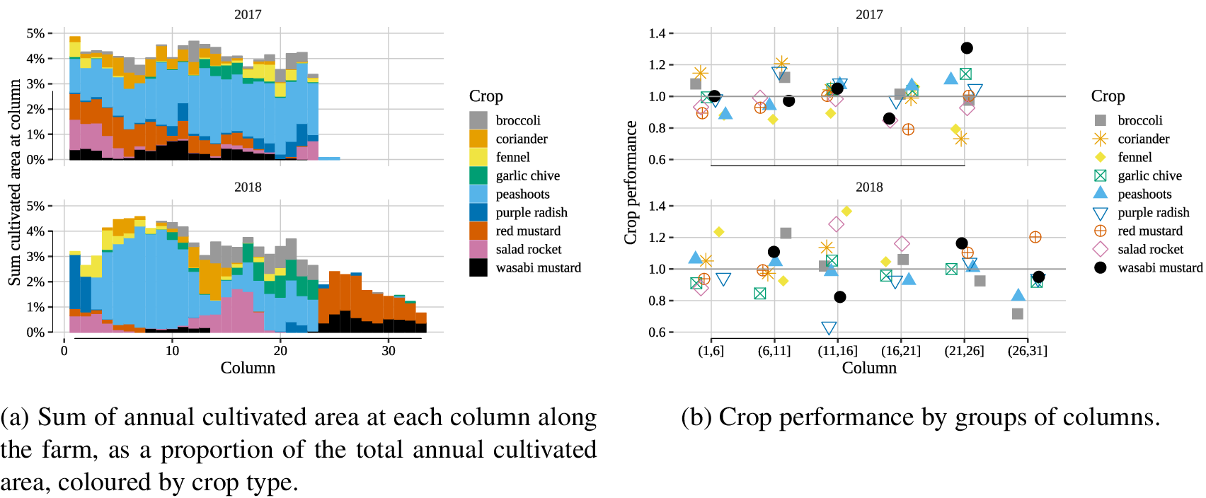
By analyzing the crop yield performance with crop location at the end of 2017, the crop performance could be judged in comparison with the crop location, and adjusted accordingly to place them in their most suited environment. For instance, salad rocket (pink), was mostly grown between columns 1 and 6 in 2017, but its crop performance was 0.93, while performance between columns 11 and 16 was 1. Consequently the following year, more salad rocket was grown between columns 11 and 16, yielding a crop performance for that zone of 1.4. Similarly, red mustard (red) had a performance of 1 at columns 21–24 in 2017, but 0.89 at columns 1–6. They were therefore likely to be suited to the back of the farm, which is warmer, so they were located at columns 25–33 in the extended farm, where they achieved a performance of 1.2 in 2018. Combining this information with an understanding of the optimal conditions, and real-time forecasts of temperatures in the farm can help GU farm operators optimize the location of each crop, and maximize the use of cultivated area.
5. Influence of Lights and Fan on Farm Environment
5.1. Heat gains from the LED lights
The LED lights have the greatest influence on daily temperature fluctuations in the farm. The temperature and RH variation between the sensors shown in Figure 10 is representative of a typical day in the farm. At the front of the farm, temperature readings are most similar to the external weather conditions as they are the closest to the incoming air. The data captured by the other four sensors located more centrally within the farm are much more similar to each other, and the temperatures follow a clear increasing pattern when the lights are switched on (5 pm), and decrease when they are switched off (11 am). The mean difference between temperature readings when the lights were on is 2.4°C as opposed to 1.1°C when the lights were off, suggesting the lights affect the temperatures in a more localized manner, but that during the day (farm night-time), there are no local heat sources and the air is sufficiently mixed. There was no such clear difference between night and day for humidity, where the difference between the sensors was on average 4.5%. There is not enough information to ascertain whether this difference in the humidity readings from different sensors is due to uneven drift of the RH sensor, or local differences in RH (Both et al., Reference Both, Benjamin, Franklin, Holroyd, Incoll, Lefsrud and Pitkin2015).
Temperatures and relative humidity measured by the five sensors and outside on 1 day (November 15, 2018). The shaded zone represents the period when the LED lights were on.

The right side of Figure 10 shows that the RH peaks to 82% when the temperatures drop during the farm nighttime. As crop transpiration rate is normally proportional to its received photosynthetically active radiation from the LED lights (Stanghellini, Reference Stanghellini1987), the lack of peak observed during the crop photoperiod suggests that transpiration levels in the farm are low. Humidity levels in the tunnel could thus be dominated by the evaporation from the irrigation process that occurs in the morning (8–10 am) and in the evening (5–7 pm) rather than transpiration. Low transpiration rates are likely because the crops grown are microgreens, with lower Leaf Area Index than mature crops (Boulard and Wang, Reference Boulard and Wang2000).
Furthermore, the high correlation of temperature with humidity (= −0.38 for top bench sensor) suggests that the air moisture content is relatively constant throughout the day (as warm air can contain more air moisture). Consequently, it seems that temperature is more important variable to control in this farm than RH.
The influence of the LED lights on temperature varies with average external temperature. Figure 11 shows the daily change in top bench temperature compared to its daily minimum as a function of the day’s average external temperature (separated in half-degree bands), estimated using kernel regression on the detrended temperature records. When the temperatures outside are colder the lights “warm” up the farm to a greater extent, and over a longer period, which can be up to 13 hr after the lights came on. For example, when external temperatures are <7°C (blue in Figure 11), the temperature inside the farm increases by over 5°C. When external temperature was over 20, temperatures in the farm would not increase by more than 5°C, and temperature increase plateaus after 4 hr. This daily shape was very similar for each sensor, but the magnitude of heating varied for each location.
Daily change of temperature from the daily minimum, for every half-degree of average daily external temperature from −5 to 30°C.

Owing to their significant influence on indoor temperatures, a useful component of the digital twin would therefore be a warning system when any additional hours of lighting would result in increasing the indoor temperatures beyond the optimal range. As aforementioned, the LED lights within the tunnel are expected to be on for 18 hr a day, and switched off for 6 hr during the day. Although this is what happens most days, there can be some variations as the farm operators will occasionally turn on the lights for additional hours to show visitors the farm, to check the lights are all working, or to clean the farm. Sometimes they will be left on by mistake.
There are no light sensors currently in the farm. Thus the actual period when the LED lights are switched on needs to be inferred from the daily energy use. A light proxy is created by assuming the lights are on if the energy use is over 0.9 times the days’ mean energy use (where a day is defined as 5 pm–11 am to correspond with the lighting period), and the energy demand is over 30 kW. The hour before the first hour the lights are on is also indicative: if energy use in any hour increases by more than 0.4 times its preceding hour, that hour is defined as the first hour of the photo-period. Based on these criteria, we estimate that the lights were turned on for the expected 18 hr photoperiod for 94% of all days monitored, and were off for 6 hr during the daytime for 13% of all days monitored (Figure 12). The duration of the photoperiod was on average 18 hr, with a standard deviation of 2.19 hr, which shows that the schedule was followed, if not exactly.
Proportion of 560 today days that the light is on according to our measure derived from energy readings, and the expected schedule.

5.2. The extraction fan
The extraction fan is controlled by an analog control dial, as shown in Figure 13a. The settings on the control dial range between 7 (off) and 5 (full power), which corresponds to air changes per hour (ACH) between 0 and 4.5. The fan settings are recorded by the farm operators daily for the last 2 years. Since the meter reading at Clapham Common only measured the energy use of fan 2, the power use ( $ P $) for each ventilation setting ( $ x $) could be derived using a power curve by analyzing the energy use at each known ventilation setting, reported in Equation (1), which has a close fit of $ {R}^2=0.95 $.
 $$ P={10}^{x/5.772}. $$
 Figure 13b shows the relationship between the energy use from the fan and the setting read from the dial. On the top x-axis, the ventilation rate in ACH is estimated using the specific fan power of 2.39, and total volume  $ \left({V}_{tot}\right) $ of tunnels the fan is connected to, and given in Equation (2). The red line in Figure 13b shows the mode of ACH for each reported ventilation setting, and how close it is to the best fit line. The advantage of a digital twin combining historic manually recorded data of the farm settings and the energy readings is apparent here: the dashboard can output ventilation rates rather than energy consumption, and advice on ventilation change can be translated into settings on the dial.
 $$ ACH={E}_{\mathrm{CC}}/ SFP\times 3600/\left({V}_{tot}/2\right). $$
The extraction fan.

Although the recorded fan settings enable us to infer the effect of changing the control setting on the energy use of the fan, the influence of the fan on the internal environment is not so clear because the fan power has been consistently changed with external temperature. This is shown in Figure 14 for temperature and RH, where the “Top bench” sensor represents conditions in the farm against Met Office weather data for St James’ Park. The x-axis shows the different ranges of energy use of the extraction fan 2 at Clapham Common between 11 am and 5 pm when the lights are off, which can be related to the speed of the fan with Equation (2). The extraction fans in the farm are generally set at lower speed (3–6 kWh) only when the external temperature is under 5°C and the RH is over 75%. The fans are on high power ( $ > $24 kWh) when the daytime external temperatures exceed 20°C. Despite this confounding effect, the results show that the fans influence internal conditions: the fan on full power ( $ > $30 kWh) controls overheating during periods of high external temperatures, as mean temperatures in the farm were on average 2 cooler than outside, with corresponding humidity levels.
Temperatures and humidity on the top bench and at St James’ Park between 10 am and 4 pm for different ranges of energy use of extraction fan 2°C at Clapham Common.

6. Data Models: Forecasting and Feedback of Farm Temperature
The added value of a digital twin over a simple monitoring and enriched data visualization system is the ability to integrate forecasting models onto the data platform. Rather than giving a simple reactive warning based on threshold temperature or energy readings, the tool can suggest targeted operational changes for the next 12 and 24 hr, and feedback on causes and effects of the farm performance and operations (Figure 1). Specifically, forecasting internal temperatures could enable the farm operators to dynamically reduce the ventilation if the farm is likely to be too cold, temporarily add a heater in a specific location, or trial different light settings. In turn, the digital twin can provide feedback on the effectiveness of the measures taken.
This differentiates from typical CEA predictive control models where the modifications to the control processes (heating, ventilation), are automatically regulated as a response to short-term temperature forecasts (Coelho et al., Reference Coelho, De Moura Oliveira and Cunha2005). Whereas this digital twin will not actuate any equipment, it can transparently provide longer term forecast and decision-making assistance with control processes that are not available in the control system (such as in this case the ventilation system and mobile heaters), and that are robust to human error (i.e., control panel being inadvertently switched off). Advice can be specific to the needs of the farm, which as we have seen in Section 4, for GU this is when temperatures are likely to exceed the temperatures of 18, 24°C.
6.1. Brief review of temperature forecasting
Until the late 90s, temperatures in greenhouses were kept at fixed setpoints, in order to keep the mean temperature within range. Chalabi et al. (Reference Chalabi, Bailey and Wilkinson1996) proposed the first real-time control algorithm to minimize energy use by combining weather forecasts with a heat and mass balance model. For typical greenhouses, Litago et al. (Reference Litago, Baptista, Meneses, Navas, Bailey and Sánchez-Girón2005) found temperatures correlated most with solar radiation, external air temperature, and ventilation rate, while humidity was most related to evapotranspiration, ventilation rate, and external relative humidity. Litago et al. (Reference Litago, Baptista, Meneses, Navas, Bailey and Sánchez-Girón2005) used these correlations to inform a statistical model of the heat and mass balance equations. Indoor “online” short-term temperature forecasts (2–3 hr) have been developed successfully for buildings using time series data, particularly with auto-regressive integrated moving average models with exogenous inputs (ARX with Moving Average [ARIMAX]) (Kramer et al., Reference Kramer, van Schijndel and Schellen2012). For greenhouses, AutoRegressive with exogenous inputs (ARX), ARMAX have been demonstrated to have good accuracy over 2–3 hr windows (3°C) (Uchida Frausto et al., Reference Uchida Frausto, Pieters and Deltour2003; Patil et al., Reference Patil, Tantau and Salokhe2008), with an external temperature being more influential than solar radiation.
More recently, neural network-based nonlinear autoregressive models were found to be more accurate than ARX in Uchida Frausto and Pieters (Reference Uchida Frausto and Pieters2004) (root mean squared error [RMSE] of 1.7°C for 1 hr horizon) and Mustafaraj et al. (Reference Mustafaraj, Lowry and Chen2011) for short-term forecasting of greenhouses and office buildings, respectively. In a more recent application to a greenhouse, Francik and Kurpaska (Reference Francik and Kurpaska2020) used Artificial Neural Networks (ANN) to forecast temperatures to reduce energy use, and achieved average RMSE values of 2.9°C over a 1 hr forecasting horizon. Zamora-Martínez et al. (Reference Zamora-Martínez, Romeu, Botella-Rocamora and Pardo2014) found that online-learning of temperature forecasts using complex ANN models had worse behaviors than with simpler models with less parameters.
The most important temperatures to predict in GU are when temperatures cross optimal bounds. Gustin et al. (Reference Gustin, McLeod and Lomas2018) showed that ARIMAX models could give reasonably accurate forecasts for extreme temperatures (RMSE = 0.82°C for a 72 hr forecast horizon) when forecasting temperatures inside a house for heat waves, to warn occupants to open windows. On the other hand, Ashtiani et al. (Reference Ashtiani, Mirzaei and Haghighat2014) compared ANN and ARX models for extreme temperatures in dwellings in Montreal and had an RMSE of 1.76 and 2.1°C, respectively, as neither model could fully capture all the parameters explaining why temperature would peak.
Although the forecasting accuracy of the models developed in the studies was good (Uchida Frausto et al., Reference Uchida Frausto, Pieters and Deltour2003; Ríos-Moreno et al., Reference Ríos-Moreno, Trejo-Perea, Castañeda-Miranda, Hernández-Guzmán and Herrera-Ruiz2007; Mustafaraj et al., Reference Mustafaraj, Chen and Lowry2010), they have been primarily developed to improve HVAC system control in air-conditioned spaces where there is detailed information available regarding their operation, and they have access to expensive variables such as transpiration rate and solar radiation to complete heat and mass balance based forecasts. As such their use cannot be directly transposed to urban-integrated farms such as GU, where space conditioning is used but operation schedules are far more unpredictable than in conventional greenhouses.
6.2. Forecasting methodology
As the farm managers tend to check the dashboard and sensor data at the beginning and end of the work-day, these are the two best times to provide a forecast. Thus, the forecasts are generated at 4 am for the first workers who arrive at 6 am to aid in decision-making of the farm operations of the day; and at 4 pm to warn and inform about the possible conditions that would happen overnight just before the workers leave while maintaining a 12 hr difference between the two forecasts. Although there are sensors in many different locations in the farm, in this demonstration stage we limit the selection of the forecasting methodology on the temperatures of the sensor at Column 18, top bench. Hereafter referred as the “farm temperature”  $ {T}_f $, this is the location with the least missing data for the entire monitoring period. The forecasting models are fitted with 1 year of the available data, as this captures the yearly and daily seasonal effects. For each new forecast, the model coefficients are thus newly fitted to the latest data available, with up to 1 year.
In this section, two forecasting models are compared: static seasonal autoregressive moving average models (SARIMA), and dynamic linear models (DLM). SARIMA models are parsimonious and have been shown to be effective in similar settings, that is, for forecasting extreme temperatures (Gustin et al., Reference Gustin, McLeod and Lomas2018). In comparison, DLM utilizes far more parameters which adds flexibility in the modeling, but may result in less stable forecasts. The SARIMA model is only trained on farm temperature data, while the DLM model also uses energy use data from the CP meter to derive the lights proxy. We compare these models to identify their suitability and fitness for the underground farm temperature prediction and feedback system on a test dataset of 24 days, evenly spread across 2018. The forecasts are only evaluated for the test datasets.
6.2.1. Static seasonal model
The SARIMA models are a family of time series models which fit linear coefficients to a time series using the Maximum Likelihood method. A SARIMA model is of the form (p,d,q) × (P,D,Q), where p is the number of auto-regressive terms, d is the order of differencing, and q is the number of moving average terms. The seasonal component captures the seasonal dynamics of the model, here set to a 24 hr period, where (P,D,Q) are the seasonal equivalents to (p,d,q). SARIMA models use differencing (terms d and D) to give a series that is stationary in mean and autocovariance. Removing the daily seasonal pattern in  $ {T}_f $ by taking one 24-hr seasonal difference, the data passed the Augmented Dickey–Fuller Test. The optimal model order for each day was identified using the auto.arima function from the forecast package (Hyndman and Khandakar, Reference Hyndman and Khandakar2008), where the model order was chosen for each version to minimize the Akaike Information Criterion (AIC). The most common order identified over 400 daily forecasts was SARIMA(3,0,2)[24](2,1,0), but this varied depending on the AIC for different model orders.
We note that as this model uses only the temperature information, it could be used when data are not captured from other sensors and monitors.
6.2.2. Dynamic linear models
SARIMA models work well in instances where the data follow a strict seasonal pattern. In this case, although the lighting schedule is designed to repeat daily, there are changes to this pattern as discussed in Section 5.1. As the data do not follow the strict seasonal pattern expected in SARIMA modeling, we also develop a bespoke modeling solution that incorporates additional data recorded in the farm.
Thus, we consider a DLM that uses a state-space approach and can explicitly allow for data-driven seasonal components. We employ a DLM with time-varying mean and changing seasonal component of the form:
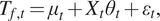 $$ {T}_{f,t}={\mu}_t+{X}_t{\theta}_t+{\varepsilon}_t, $$
where  $ {T}_{f,t} $ is the farm temperature at time $ t $. The mean varies according to a random walk $ {\mu}_t={\mu}_{t-1}+{\nu}_t $ with $ {\nu}_t\sim N\left(0,{\sigma}_{\mu}^2\right) $, as do each of the seasonal state variables, $ {\theta}_{t,i}={\theta}_{t-1,i}+{u}_{t,i} $ with $ {u}_{t,i}\sim N\left(0,{\sigma}_i^2\right) $. For a comprehensive introduction to dynamic modeling of time series see West and Harrison (Reference West and Harrison1997).
The time-varying mean,  $ {\mu}_t $, represents a base temperature within the farm which we expect to be related to external temperature and ventilation. Generally, a DLM features a seasonal component with a fixed frequency contribution, such as a 24-hr cycle similar to the SARIMA model. Rather than using a traditional fixed frequency seasonal component, we apply a data-driven component, $ {X}_t $, that contains the information about the lighting schedule inferred from the energy meter readings, without referring to the time of day or expected photo-period cycle. $ {X}_t $ has entries indicating the hour in the photo-period to which $ t $ corresponds to (i.e., the $ n $th hour that the lights are on or off). This allows for changes to the scheduled lighting such as the lights being switched on earlier, or for longer, to be explicitly modeled in this DLM. The inferred lighting schedule is generated using the energy meter readings, as described in Section 5.1. This Lights proxy can also be used to forecast future temperatures under different conditions, either with the typical lighting schedule or the actual lighting settings that occurred in that time period, inferred from the energy readings. Although in reality, the future energy readings are not available, changes to the lighting schedule may be known in advance so that this type of forecast can be generated.
Bayesian inference was used for fitting this model and generating predictions. Conjugate inverse-Gamma prior distributions are used for the variance components  $ {\sigma}_{\mu}^2 $ and $ {\sigma}_i^2 $ and MCMC inference is performed using the bsts package (Scott, Reference Scott2020). Inference on the state components is performed using 1,000 iterations of the chain, and the first 200 iterations are discarded as burn-in.
By allowing the state components in  $ {\theta}_t $ to evolve over time we can capture the behavior shown in Figure 11, as the lights cause different rates of increase and decrease in $ {T}_f $ according to the external temperature. If $ \theta $ were constant then features such as a plateau in temperatures being reached quicker in summer would not be captured, as in that case the daily component would not change through the year.
Using output of the DLM we can thus investigate the posterior distribution of these lighting components at different times of year. In Figure 15 the change of temperature from the previous hour is plotted for the following cases: after the lights have been turned on for one, and for 5 hr (left and middle panels), and in the first hour of being turned off (right panel). They are separated for the months of February, June, and October 2018, where the corresponding average outdoor are 6.7, 18.6, and 11.1°C. From this plot, the different effects over the year of the lights on temperature can be seen, which is in agreement with Figure 11. The model fits a greater increase in temperature for the first hour the lights are on in June compared to the other months. The change of temperature for the fifth hour the lights are on is less on the warmer days compared to February, as when it is colder the farm temperature takes a greater number of hours after the lights are turned on to reach a plateau. In contrast, the decrease in temperature on the first hour the lights are switched off is greater in February than in the warmer months. Using a model with changing lighting component parameters thus allows for these changes to be modeled.
Temperature changes from the previous hour when the lights have been on for 1 hr (left), 5 hr (middle), and for the first hour without lighting (right), for February, June, and October.

This model is flexible and able to accommodate changes in the operating conditions, such as external temperature and ventilation settings, without explicitly modeling them.
6.3. Evaluation criteria
The model is evaluated on a test dataset of 24 days, the 1st and 15th of every month in 2018. The test dataset is chosen to be evenly spread out over the year to check if the performance changes despite the different conditions in the farm over the year (i.e., different ventilation, lighting schedules, and weather). Only 24 forecasts are generated because the average running time of the DLM model is 25 min, even though the SARIMA model is much faster (2.8 min on average). The focus of the statistics is on the forecasting horizon to assess the performance of the models had they been implemented in real-time. The different forecasts from the DLM models are thus compared with forecasts from the SARIMA model for each of these days. We also compare the forecasts from the two models against a naive forecast repeating the previous day’s observations. The summary statistics are reported in Table 2, over a 48 hr forecasting horizon, for the morning and afternoon forecasts. The prediction performance of the models is evaluated in terms of general fit using the RMSE, mean absolute error (MAE), mean bias error (MBE), and coverage rate (CR) when estimating whether the temperatures on the following day will escape the desired 18–24°C interval.
Mean statistic of 24 daily forecasts of the four following models (1st and 15th of every month in 2018): (a) the previous 24 hr as forecast, (b) Seasonal Arima model, (c) DLM model using observed light pattern, (d) DLM model using the typical light pattern expected for the given day. Bold values highlight the statistic suggesting the most accurate model type. Standard deviation from the mean of the statistic across forecasting days are included in parentheses.
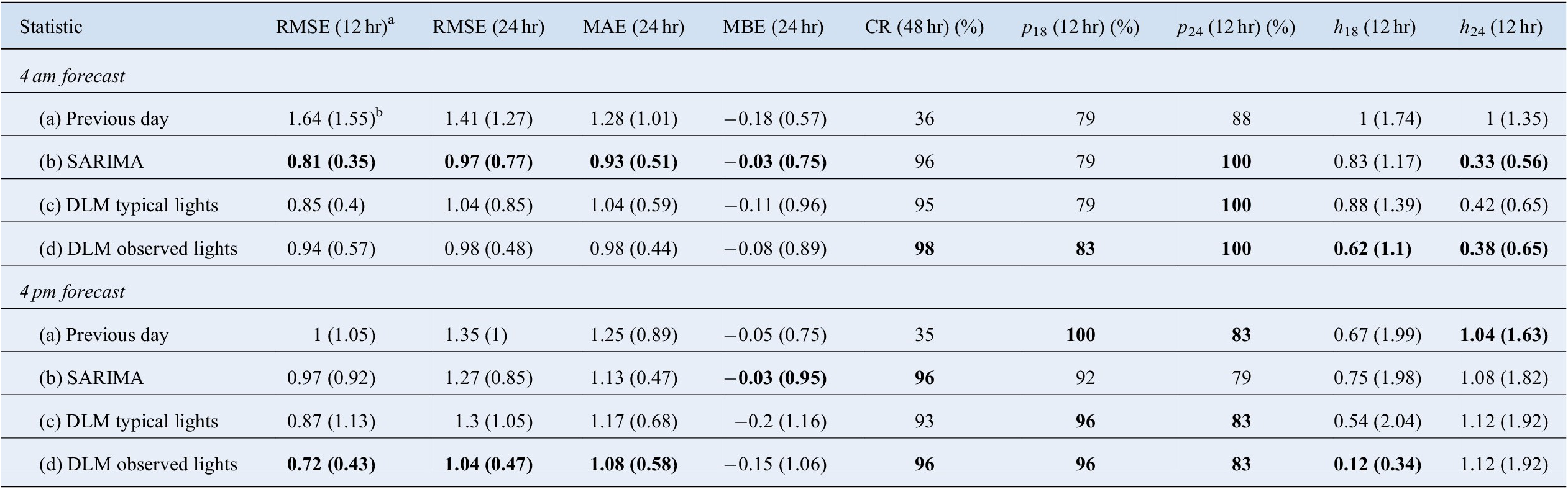
Note. Units in °C.
Abbreviations: CR, coverage rate; DLM, dynamic linear models; MAE, mean absolute error; MBE, mean bias error; RMSE, root mean squared error; SARIMA, seasonal autoregressive moving average models.
a Forecast horizon over which statistic was calculated.
b Standard deviation from the mean of statistic over forecasted days.
The metrics are defined in Equations (4)–(6), where  $ {y}_p $ denotes the predicted temperature and $ {y}_o $ the observed temperature, and $ N $ is the number of hours over which the statistic is computed. RMSE is the most commonly reported metric for assessing model performance. It gives more weight to the largest errors by taking the square of the residuals, which is desirable in this case as the focus is on capturing extreme temperatures as accurately as possible.
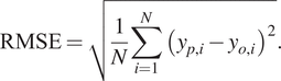 $$ \mathrm{RMSE}=\sqrt{\frac{1}{N}\sum \limits_{i=1}^N{\left(\hskip0.1em {y}_{p,i}-{y}_{o,i}\hskip0.1em \right)}^2}. $$
Some analysts judge the MAE, which represents the average magnitude of the residuals, to be a more precise performance indicator (Willmott and Matsuura, Reference Willmott and Matsuura2005; Chai and Draxler, Reference Chai and Draxler2014).
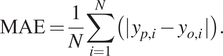 $$ \mathrm{MAE}=\frac{1}{N}\sum \limits_{i=1}^N\left(|\hskip0.1em {y}_{p,i}-{y}_{o,i}\hskip0.1em |\right). $$
The MBE indicates the systematic error of the model to over or under forecast.
 $$ \mathrm{MBE}=\frac{1}{N}\sum \limits_{i=1}^N\left(\hskip0.1em {y}_{p,i}-{y}_{o,i}\hskip0.1em \right). $$
 The CR corresponded to the percentage of estimated points which fell within the 95% confidence or credible interval (CI). For the naive forecast using the previous day, the CI is estimated using  $ \sigma $ the standard deviation of the temperatures from the previous day as $ \pm 1.96\sigma /\sqrt{48} $ from the forecast temperature.
For GU it is also important to know whether the temperatures will escape the desired temperature interval, when, and for how long. To predict these probabilities, for the SARIMA model, we forecast using bootstrapped values of the error distribution, and averaged the number of these bootstrapped forecasts that were over 24°C and under 18°C. We could thus compare the forecasts with the mean number of hours that were predicted wrongly to be under 18°C  $ \left({h}_{18}\right) $, or over 24°C $ \left({h}_{24}\right) $. These could be also estimated from the probability distribution output from the DLM forecasts. To compare the calibration of this probability, we report the proportion of forecasts where a probability greater than 0.7 correctly predicted that the temperature crossed 24°C $ \left({p}_{24}\right) $, or 18°C $ \left({p}_{18}\right) $, and that a probability less than 0.7 gave a true negative. For the naive forecast, the probability is taken as 1 if the temperatures on the previous day crossed either threshold within the same 12 hr window as the forecast.
6.4. Model comparison
The accuracy of temperature predictions based on the DLM with inferred photo-period is compared with the predictions of the DLM using the fixed lighting schedule. We also compare the predictions against the SARIMA model presented in the previous section (Figure 16). The statistics taken on the prediction errors for each of these forecasts are presented in Table 2.
Plot of 24-hr forecast from 4 pm (hour 0), with 24 hr preceding, for lowest and highest RMSE values. Top: Hourly external temperature (orange), overlayed with 24 hr average (black). Middle: Predictions against observed data, with annotated message output for farmers, indicating if temperature was higher or lower than expected in 12 hr forecast horizon. Bottom: Values of fan 1 and 2 are estimated ACH (Equation (2)). Lights proxy and energy from lights are dimensionless.

The performance of the SARIMA model and the DLM with typical lights (models b and c respectively in Table 2) is quite similar, and the model fit for 24 hr performed well compared with previous forecasting models for greenhouse temperatures, with an average RMSE under 1.3°C for all predicted days. For the 12-hr morning forecasts, SARIMA (RMSE = 0.81°C) outperformed the DLM model with observed lighting (RMSE = 0.94°C). On the other hand, this DLM improved upon the SARIMA model for the afternoon forecast (RMSE = 0.72 compared with 0.97°C). As the DLM explicitly uses the lighting schedule, it is fitting that the DLM should be better than SARIMA in the afternoon forecast, just before the lights are expected to turn on at 5 pm.
Both SARIMA and DLM models had significantly better fits than the naive forecast, which has comparatively high RMSE values. Only 36% of observed temperature fell within the CI with the naive method, compared to 94% on average for all the other models. This demonstrates both the SARIMA and DLM models add valuable accuracy to the temperature forecasts.
Comparisons between the SARIMA and DLM forecasts for days with the five lowest RMSE values (<0.56°C) in Figure 16a, and for the 5 days with the highest RMSE values (RMSE > 1.94°C) in Figure 16b. Each figure is divided into three panels, A, B, and C. The x-axis denotes the hour count from 4 pm, where 0 is the first hour of the forecast. Panel A shows the hourly external temperature in orange, with its average daily mean in black. Panel B presents the farm temperature (black dashed line), and the forecasts from the three different models: SARIMA, DLM typical lights (with the typical light schedule), and DLM observed lights (with the inferred light schedule from the lights proxy). The interpretations of lights and fan power from the energy meter readings are plotted in panel C. The black and orange lines are the estimated ACH of fan 1 and fan 2, respectively, calculated from Equation (2). Their extent is marked on the y-axis, from 0 ACH (no ventilation) to 4.5 ACH (max ventilation). The lights pattern is also indicated on panel C, where 4 on the y-axis indicates the lights are on (lights proxy in pink). The estimated energy use of the lights is also plotted, where 30 kWh is normalized to 4 to show how the lights proxy captures the lighting condition from the meter readings (see Section 5 for details).
The similarity between the SARIMA and DLM models in Figure 16a shows that when the lighting schedule is close to what is expected, the simpler SARIMA model would suffice for prediction. However, on January 15, 2018, plotted in Figure 16b, the benefit of the added complexity of DLM can be seen, as there is the ability to closely forecast the effect of turning the lights on later than expected. Indeed, the lights proxy in panel C shows the lights were off for 18 hr rather than the typical 6 hr. The difference between predictions based on inferred lighting from observed data and the typical lighting schedule shows that the data-centric lighting component is utilized in the dynamic model. The inferred lighting schedule improves the accuracy of the prediction compared to the observed values in almost all statistics of Table 2 (model d).
While the forecast is close to the observed temperatures for typical days across all models, the predictions from the dynamic model are better at capturing the extreme temperatures reached in the farm, exemplified by the  $ {p}_{18} $ and $ {p}_{24} $ statistics giving more accurate temperature warnings than the SARIMA model.
In general, the forecasting performance of the SARIMA and DLM modeling are similar. However on days with atypical lighting (or in the days following atypical lighting) the DLM approach gives more accurate prediction. In addition, this model could be used to simulate the effect of different lighting schedules without carrying out the experiment in practice.
6.5. Application of forecasting model to aid decision-making
Whilst the temperature forecasting alone is useful, more insight can be gained when combined with a feedback system in this digital twin framework. The forecasts and live temperature readings can be compared, and discrepancies identified in real-time. For instance, when running the SARIMA forecasts for 400 consecutive days, we found that all days where temperatures were uncharacteristically badly predicted were linked to an uncharacteristic change of external temperature, energy use, or door setting. This is shown in Figure 16b in the subplots for January 15, 2018, when the bias (−5.46°C) was significantly larger than the next largest bias (−0.83°C), and is linked to an extended nighttime period in the farm.
Feedback would include a warning that temperatures are lower than the forecast and therefore changes to heating and ventilation should be made so crop growth is not impacted, such as the bias messages in panel B of Figure 16. For illustration, in the subfigure of Figure 16a for 1st November October 2018, the forecast issued at 4 am would include a warning message that temperatures were 0.31°C lower than forecast in the previous 12 hr, despite a 2.5°C increase in external temperature, and no apparent change in controls (fan 1 and fan 2 have constant ACH and the lighting pattern was as scheduled). While this shows the models captured the increasing trend in external temperature, the forecast error shows that some farm controls were not predicted. In this case, the lower temperatures could be due to inadvertently open doors somewhere in the farm, and thus trigger a warning. Over time, additional variables can be incorporated into the forecast model according to the feedback generated by comparing the forecasts and observed temperatures.
Various operational processes in the farm changed throughout the model testing period (see Section 5) which have excited the training data, but the data-centric modeling has shown to be resilient to such change, as the forecast error did not vary significantly over the testing period. As such, the dynamic model is particularly valuable in this start-up environment, as it is flexible to the changing operations due to its time-varying mean  $ {\mu}_t $, which can account for the varying external temperature and ventilation. By separating the trend with the effect from the lights, the DLM methodology can also be used to test the effect of different lighting schedules, enabling farm operators to make better-informed decisions. This overcame one of the limitations of the dataset, where the effect of weather and ventilation appeared to be correlated. Although the growing lights were on for 18 hr the majority of days, there was variation of the time at which the lights came on and off. For instance, our lights proxy estimates the lights came on an hour later than planned 26% of the time, and came off with an hour earlier 46% of the time (Figure 12). As such, the training data were excited to a reasonable extent to assume the robustness of this methodology to predict typical conditions.
The conditions in the farm are not subject to an automatic control system, but managed manually by farm operatives. Therefore information such as the power increase of using the extraction fan and the probability of high temperatures can be used in combination to make informed decisions about what changes should be made in the farm. As these changes can only be applied during the working day in the farm, the model can also aid decision-making about whether automating certain equipment would be worth the additional cost, as then changes could occur when operatives are not present. Furthermore, as in the case of January 15, 2015 when the lighting system was left on “manual” by mistake, the model can warn the user about the failure of the control system, as well as its effect on environmental conditions, and relate these to the potential crop growth outcome. Although automation helps, having this extra level allows to catch and understand the implications of inevitable manual errors and unprecedented change.
7. Discussion
The digital twin presented here proposes a framework for urban-integrated farms to collect data and use it meaningfully. Unlike current visualization dashboards or CEA systems, we presented an integrated system linking a broad data collection system, with tailored data analytics and modeling.
A key challenge for a successful digital twin is continuous data collection. However, not all information can be tracked with sensors, and we presented a method for combining data from different sources into a database, and inferring operational changes in GU. We then showed how historic data could create a virtual representation of the farm operations and environment. Previous models forecasting environmental conditions in greenhouses tend to show much more yearly seasonal variation with external weather conditions, but in GU, the artificial lighting has the strongest influence on temperature, causing an indoor diurnal pattern opposite to the external daily temperature pattern, which complicates the use of traditional seasonal decomposition techniques as many explanatory variables are confounded. The buffer effect of depth further meant that the influence of external temperature was less than conventionally found. We found that forecasting temperatures in the farm were best achieved with a DLM featuring a time-varying mean with a data-centric lighting component. Although there is a vast literature in temperature forecasting, the variety in performance of different models for similar environments highlights the need to create bespoke models that are suited to the specific environment, user needs, and data available.
Digital twins rely on a constant stream of input data, and thus robust network connectivity, a long-term sensor maintenance plan, and a diverse data collection system. Innovative projects, such as this urban-integrated hydroponic farm, are unlikely to have fully controlled systems as farm operators learn how to use their unique environments. This leads to changes which can be tracked through observed data. For example, the base energy usage increased in 2018 as the farm was extended, and more lights became “online.” Monitoring a few variables from the beginning allows to identify other key variables that would be useful at a later stage: here, further sub-meters could improve forecasting accuracy. Digital twins thus need to be built with resilience and flexibility in mind, to add new sensors as funding and technology become available. For instance, future work will include incorporating light sensors that were added at a later date in the farm, to replace the light proxy used in the DLM forecasts.
The main limitation of data-centric models in commercial environments is that they can only forecast and feedback on eventualities that have happened. Were the farm to test different lighting regimes at different times of day, and different ventilation rates over prolonged periods of time in different weather conditions, more could be learned about the response of the farm environment to controls. However, the realities of a commercial CEA imply that operators will always try to keep conditions within their optimal ranges, whether this is done automatically through control systems, or partially manually as in this case. The benefit of digital twins is to provide an “extra level,” where unexpected changes can be tracked, as well as their effect on other variables (e.g., ventilation on too high). By being a virtual extension of the reality in the farm, it also allows to compare current conditions with historical data to provide meaningful information to assist in decision-making.
In this paper, we showed the challenges and opportunities of creating a digital twin, which lie in data collection, data interpretation, and tailored modeling. As opposed to simple data visualization, digital twins provide an opportunity to enhance the data by outputting inferred data fields. Bespoke models can be implemented on a platform that can harness the breadth of data collection, be it structured or unstructured. While this prototype is addressed to urban-integrated farming, it serves as an example for digital twins of non-standard physical environments and processes. We argue that more standard environments, such as traffic systems or construction processes, may benefit more from off-the-shelf software which represents the process well. Digital twins are particularly useful in environments where the specifics of the process are not so well understood (e.g., in buildings, for representations of a street). In such cases, data-centric methods are pertinent because they can represent the unobservable states through data streams, and thus provide additional insight. The framework described here is suited to mid to large scale processes, often seen in civil engineering, where sensor maintenance will also be an issue and several processes will be of concurrent interest. As every environment is different, digital twins are an opportunity to move away from “one size fits all” approaches and tailor the information display to match needs and available data.
Funding Statement
This work was supported by the Engineering and Physical Sciences Research Council grant EP/L016095/1. KL carried out this work at the University of Warwick and was supported by Engineering and Physical Sciences Research Council grant EP/R034710/1. This work was also supported by AI for Science and Government (ASG), UKRI’s Strategic Priorities Fund awarded to the Alan Turing Institute, UK (EP/T001569/1), and the Lloyd’s Register Foundation program on Data-Centric Engineering.
Competing Interests
The authors declare no competing interests exist.
Data Availability Statement
The temperature data can be accessed upon request. However, the crop growth, operational controls, and energy use data are proprietary of Growing Underground for commercial purposes. Please contact the authors if you would like a copy of synthetic data in order to replicate the findings.
Author Contributions
Conceptualization, R.C., M.J.-S., and K.L.; Methodology, M.J.-S. and K.L.; Software, M.J.-S. and K.L.; Validation, M.J.-S. and K.L.; Formal analysis, M.J.-S. and K.L.; Investigation, M.J.-S. and K.L.; Resources, M.J.-S.; Data curation, M.J.-S.; Writing original draft, M.J.-S. and K.L.; Writing revision and editing, R.C., M.J.-S., and K.L.; Visualization, M.J.-S. and K.L.; Supervision, R.C. and M.G.; Project administration, R.C. and M.G.; Funding acquisition, R.C., M.G., and M.J.-S.
Acknowledgments
We would like to thank Paul Fidler, for his invaluable assistance setting up the WSN, and the staff at GU, for their long-standing collaboration and enthusiastic support throughout the entire project and beyond.


 Open access
Comments
No Comments have been published for this article.