


1. Introduction
Mortality forecasting is central to actuarial science, public health,and policy planning. Traditional methods such as the Lee–Carter model (Lee & Carter, Reference Lee and Carter1992) relied on historical mortality rates in an autoregressive setting to capture long-term trends. Although these conventional approaches have proven valuable at an annual and country-level scale, they remain less equipped to handle the spatial heterogeneity and rapid changes that arise from short-term environmental variations.
The escalating concern surrounding climate change by regulators has demonstrated the need to integrate climate variables into mortality models (EIOPA, 2021). Environmental factors such as temperature, humidity, and precipitation can significantly influence weekly mortality rates (Carleton et al., Reference Carleton, Jina, Delgado, Greenstone, Houser, Hsiang, Hultgren, Kopp, McCusker, Nath, Rising, Rode, Seo, Simcock, Viaene, Yuan and Zhang2022). Yet, their explicit integration into short-term actuarial contexts remains relatively limited. To address this gap, Robben et al. (Reference Robben, Antonio and Kleinow2024) introduced a fine-grained death rate modeling approach that used XGBoost to link anomalies to weekly death deviations from a Serfling-type baseline. This approach demonstrated the critical role of temperature extremes; however, it also revealed two main challenges. First, the Serfling approach predefined the pattern; the baseline model relies on fixed Fourier series for seasonality and trends. Second, the Serfling plus XGBoost framework still depends on manually engineered features.
In this paper, we introduce MortFCNet, a deep-learning method designed to forecast weekly death rates from region-specific weather inputs, to address the two challenges. Deep neural networks can be particularly well-suited to automatically extracting patterns from time-series data and capturing complex non-linear relationships between death rates and external factors. MortFCNet is capable of learning these complex relationships directly from data and, moreover, achieves this without manual feature engineering. This is a crucial consideration as effective feature engineering can be very hard to accomplish manually. In addition, we demonstrate the consistency of MortFCNet performance.
Experiments are conducted on the data from over 200 NUTS-3 regions in France, Italy,and Switzerland. The Nomenclature of Territorial Units for Statistics (NUTS) is a hierarchical system for dividing up the economic territory of the European Union for statistical purposes, and NUTS-3 represents the smallest regional level. First, we demonstrate that MortFCNet outperforms both a standard Serfling-type baseline and XGBoost, yielding superior predictive performance in mean squared error (MSE) on weekly death rates overall and per country. Second, our ablation study confirms that MortFCNet can automatically learn and transform relevant inputs from raw time-series data, thus avoiding the heavy overhead of manual feature creation. Additionally, ablation shows that MortFCNet is reliable with different hyperparameter settings.
The remainder of this paper is organized as follows. Section 2 provides an overview of existing mortality models and their extensions involving environmental variables. Section 3 introduces the notation and data sources used. Section 4 details the methodology, focusing on the MortFCNet architecture and how it compares to the baseline and a machine learning method (XGBoost). Section 5 discusses the experimental setup and key results, with an emphasis on model performance and ablation studies. Finally, Section 6 summarizes the main findings and discusses some future work.
2. Related work
Mortality forecasting models have historically relied on long-term historical mortality data to capture broad demographic trends. One of the most influential approaches is the Lee–Carter model (Lee & Carter, Reference Lee and Carter1992), which uses an autoregressive structure on single country-level mortality rates. While highly effective at modeling mortality, Lee–Carter does not incorporate region-specific or external factors, which may influence mortality prediction. More recently, researchers have developed extensions of Lee–Carter that better handle age-cohort interactions. For example, Cairns et al. (Reference Cairns, Blake and Dowd2006) introduced cohort effects and Plat (Reference Plat2009) proposed a model that integrated age, period,and cohort effects to improve mortality projections.
In actuarial research, there has been a growing interest in leveraging deep learning to enhance forecasting accuracy and flexibility. For instance, Richman & Wüthrich (Reference Richman and Wüthrich2021) extended the Lee-Carter model by introducing neural networks for multiple-population mortality data, thereby automating feature extraction and simplifying model deployment. Likewise, Perla et al. (Reference Perla, Richman, Scognamiglio and Wüthrich2021) demonstrated that neural networks, including a shallow 1D Convolutional Neural Network, effectively capture complex temporal dependencies in mortality rates. Zhang et al. (Reference Zhang, Chen and Liu2022), Scognamiglio (Reference Scognamiglio2024), Euthum et al. (Reference Euthum, Scherer and Ungolo2024), and Hsiao et al. (Reference Hsiao, Wang, Liu and Kung2024) have also applied neural networks to model and predict mortality rates across various populations.
The interpretability of deep learning applications in mortality forecasting has been explored by Hainaut (Reference Hainaut2018) using a neural-network autoencoder, where the decoder reconstructed age profiles that closely resemble the Lee-Carter coefficients. Building on this theme, Richman & Wüthrich (Reference Richman and Wüthrich2023) proposed LocalGLMNet, which retains the additive form of a Generalized Linear Model while allowing non-linear weight estimation. The LocalGLMNet model was subsequently applied to mortality forecasting by Perla et al. (Reference Perla, Richman, Scognamiglio and Wüthrich2024). While the above work focuses on all-cause mortality, Tanaka & Matsuyama (Reference Tanaka and Matsuyama2025) introduced an interpretable neural network for cause-of-death mortality forecasting, substituting the Lee-Carter tensor factorization with a one-dimensional convolutional autoencoder. This convolutional design allows parameter sharing and enables the model to learn dependencies between multiple causes of death. These approaches have demonstrated enhanced interpretability and an improved ability to capture complex patterns in mortality data. For a review of mortality forecasting using deep models, see Zheng et al. (Reference Zheng, Wang, Zhu and Xue2025), which summarizes developments by model architecture and discusses both performance and interpretability.
Despite these improvements, the role of environmental factors in mortality forecasting remains relatively understudied in the actuarial domain. Emerging evidence suggests that variables such as temperature, precipitation, and air quality significantly influence mortality risk, particularly among older populations (Carleton et al., Reference Carleton, Jina, Delgado, Greenstone, Houser, Hsiang, Hultgren, Kopp, McCusker, Nath, Rising, Rode, Seo, Simcock, Viaene, Yuan and Zhang2022). This aligns with directives from regulatory bodies, which encourage insurers to integrate climate change scenarios into risk assessments (EIOPA, 2021). In parallel, tools such as the Actuaries Climate Index (https://actuariesclimateindex.org) provide a means of assessing climate-related risks but often lack the granularity needed for precise mortality analysis. This shows the potential to combine higher-resolution datasets and advanced modeling techniques to better understand the relationship between environmental factors and mortality.
Several studies have begun exploring ways to incorporate exogenous predictors into multi-population mortality models. Dimai (Reference Dimai2025) aimed to enhance mortality forecasting by developing a multi-population mortality model that integrates environmental, economic and lifestyle factors. The study leveraged annual mortality data from the Human Mortality Database (www.mortality.org) alongside detailed socio-economic indicators and environmental variables (including temperature anomalies and air quality metrics). Robben et al. (Reference Robben, Antonio and Kleinow2024) investigated weekly mortality rates across more than 500 NUTS-3 regions in 20 European countries, augmenting a Serfling-type seasonal baseline with XGBoost to model deviations driven by weather and pollution anomalies. They used high-resolution datasets from the Copernicus Climate Data Store (Cornes et al., Reference Cornes, van der Schrier, van den Besselaar and Jones2018) and the Copernicus Atmospheric Monitoring Service (https://atmosphere.copernicus.eu), ensuring region-specific seasonal mortality trends were captured. Although their approach successfully identified short-term deviations from the baseline, it tended to overestimate mortality in certain regions (generalization challenge). Furthermore, while Robben et al. (Reference Robben, Antonio and Kleinow2024) included environmental data (weather and pollution variables) through an XGBoost extension of the Serfling baseline, the baseline model itself did not incorporate these inputs. Thus, the overall framework still relied heavily on pre-engineered features and a separate baseline calibration stage.
Building on the work of Robben et al. (Reference Robben, Antonio and Kleinow2024), we aim to explore how deep learning can enhance mortality rate forecasts using exogenous predictors, and learn patterns directly from time-series inputs, reducing the need for manual feature design and additional calibration steps. Considering computational constraints, we will focus on weather data, as the hourly air pollution data employed by Robben et al. (Reference Robben, Antonio and Kleinow2024) involved substantial processing overhead. We will focus on 3 European countries (around 200 NUTS-3 regions). Nevertheless, we will ensure consistency in datasets to enable a fair comparison across methods during experiments.
3. Notation and data
3.1. Notation
To formalize the discussion on weekly death rate forecasting, we introduce the following notations. Let $y_{a,t,v}^{(g)}$
be the observed death count in region
$y_{a,t,v}^{(g)}$
be the observed death count in region $g$
and age group
$g$
and age group $a$
during ISO week
$a$
during ISO week $v$
of year
$v$
of year $t$
, and let
$t$
, and let $N_{a,t,v}^{(g)}$
represent the exposure-to-risk, which quantifies the population at risk in region
$N_{a,t,v}^{(g)}$
represent the exposure-to-risk, which quantifies the population at risk in region $g$
and age group
$g$
and age group $a$
over the same week. The ISO week date system defines a week as starting on Monday and ending on Sunday, with the first week of the year being the one that contains the first Thursday of the year (International Organization for Standardization, 2004). This ensures consistent week numbering across years between different data sources.
$a$
over the same week. The ISO week date system defines a week as starting on Monday and ending on Sunday, with the first week of the year being the one that contains the first Thursday of the year (International Organization for Standardization, 2004). This ensures consistent week numbering across years between different data sources.
We assume each region $g$
belongs to a set of NUTS-3 regions
$g$
belongs to a set of NUTS-3 regions $\mathcal{G}$
. Each year
$\mathcal{G}$
. Each year $t$
belongs to a set
$t$
belongs to a set $\mathcal{T}$
, and each ISO week
$\mathcal{T}$
, and each ISO week $v$
is an element of a set
$v$
is an element of a set $\mathcal{V}_t$
(52 or 53 weeks per year).
$\mathcal{V}_t$
(52 or 53 weeks per year).
3.1.1. Weekly death rate
The weekly death rate, denoted by $r_{a,t,v}^{(g)}$
, is defined as
$r_{a,t,v}^{(g)}$
, is defined as
 \begin{equation} r_{a,t,v}^{(g)} = \frac {y_{a,t,v}^{(g)}}{N_{a,t,v}^{(g)}}. \end{equation}
For consistency with Robben et al. (Reference Robben, Antonio and Kleinow2024), we focus on older age groups (i.e., 65+ years) and drop the $a$
subscript later where data are aggregated.
$a$
subscript later where data are aggregated.
3.1.2. Weekly mortality rate
The mortality rate, $q_{a,t,v}^{(g)}$
, represents the probability that an individual in region
$q_{a,t,v}^{(g)}$
, represents the probability that an individual in region $g$
and age group
$g$
and age group $a$
, alive at the start of week
$a$
, alive at the start of week $v$
, will die during the week. Assuming a constant force of mortality within the week,
$v$
, will die during the week. Assuming a constant force of mortality within the week, $q_{a,t,v}^{(g)}$
can be estimated as
$q_{a,t,v}^{(g)}$
can be estimated as
 \begin{equation} q_{a,t,v}^{(g)} \approx 1 - \exp \left ( -\mu _{a,t,v}^{(g)} \right ), \end{equation}
where the force of mortality, $\mu _{a,t,v}^{(g)}$
, is defined as the instantaneous rate of death at any given point in the week, conditional on surviving up to that point.
$\mu _{a,t,v}^{(g)}$
, is defined as the instantaneous rate of death at any given point in the week, conditional on surviving up to that point.
3.1.3. Relationship between death rate and mortality rate
Under standard assumptions (constant risk of death during the week), when weekly death rates are small, the approximation $\mu _{a,t,v}^{(g)} \approx r_{a,t,v}^{(g)}$
is often sufficient. Hence, one may apply
$\mu _{a,t,v}^{(g)} \approx r_{a,t,v}^{(g)}$
is often sufficient. Hence, one may apply
 \begin{equation} q_{a,t,v}^{(g)} = 1 - \exp \left ( -r_{a,t,v}^{(g)} \right ), \end{equation}
to convert from the weekly death rate to the weekly probability of mortality.
3.2. Data sources
For consistency with Robben et al. (Reference Robben, Antonio and Kleinow2024), we use the same data sources for Death Counts, Exposure-to-Risk, Weather Data, and Geographical Coordinates in this study. Note that the hourly Pollution data are excluded from this study due to computational constraints. Specifically, we use data from three countries: Switzerland (CH), France (FR), and Italy (IT). The three selected countries share boundaries for models to incorporate potential neighborhood effects and provide sufficient regions (200+) for experimentation. In particular, Italy with 98 regions, France with 96 regions, and Switzerland with 23 regions. We will conduct the same pre-processing on the data and use the same dataset for our models to keep a fair comparison. In addition, our dataset spans from 2013 to 2019, and is divided into the training data covering 2013–2018, and the test data for the year 2019.
3.2.1. Death counts
Death counts were obtained from Eurostat (https://doi.org/10.2908/DEMO_R_MWEEK3), covering weekly deaths by sex, 5-year age group, and NUTS-3 region across three European countries: Switzerland, France, and Italy. We use death counts for individuals aged 65+ and aggregate the data across sexes (unisex). These weekly counts form $y_{t,v}^{(g)}$
in our notation.
$y_{t,v}^{(g)}$
in our notation.
3.2.2. Exposure-to-risk
Weekly exposure is denoted as $N_{t,v}^{(g)}$
for individuals aged 65+ in each NUTS-3 region. We use two main data sources for the population.
$N_{t,v}^{(g)}$
for individuals aged 65+ in each NUTS-3 region. We use two main data sources for the population.
Firstly, for the calculation of weighted weather-related variables, we leverage high-resolution gridded population data from the Socioeconomic Data and Applications Center (Center for International Earth Science Information Network, CIESIN) as the weighting factor. Specifically, we employ the population count dataset at a spatial resolution of 2.5 arc-minutes (approximately 5 km). This fine-scale grid allows us to construct population weights that reflect the spatial distribution of inhabitants within each NUTS-3 region, ensuring that regional weather averages are representative of where people actually live.
Secondly, to derive the denominator for death rates in each region, we rely on annual population counts from Eurostat. Rather than assuming a uniform population distribution over the year as was used by Robben et al. (Reference Robben, Antonio and Kleinow2024), we adopt a simple weekly update mechanism as a more practical approach used in the industry. At the start of each ISO week $v$
(for
$v$
(for $v \ge 2$
), we update the population as
$v \ge 2$
), we update the population as
 \begin{equation} \text{population}_{t,v}^{(g)} = \text{population}_{t,v-1}^{(g)} - y_{t,v-1}^{(g)}, \end{equation}
where $y_{t,v-1}^{(g)}$
denotes the total deaths in region
$y_{t,v-1}^{(g)}$
denotes the total deaths in region $g$
during the previous week
$g$
during the previous week $v-1$
. Given the relatively large population sizes and typically low weekly death counts, this method yields mortality rates extremely close to those derived from a purely uniform approach. Hence, any discrepancy in calculating weekly exposures is negligible.
$v-1$
. Given the relatively large population sizes and typically low weekly death counts, this method yields mortality rates extremely close to those derived from a purely uniform approach. Hence, any discrepancy in calculating weekly exposures is negligible.
Finally, the total person-weeks at risk of death are approximated as
 \begin{equation} N_{t,v}^{(g)} = \frac {\text{population}_{t,v}^{(g)} + \text{population}_{t,v-1}^{(g)}}{2 \times 52.18}. \end{equation}
Here, 52.18 represents the assumed number of weeks in a year, accounting for the fact that exposure is measured in weekly units.
3.2.3. Weather data
Weather data are from the Copernicus Climate Data Store (CDS) (Cornes et al., Reference Cornes, van der Schrier, van den Besselaar and Jones2018). Weather variables include daily maximum, average, and minimum temperature ( $T_{\text{max}}, T_{\text{avg}}, T_{\text{min}}$
), relative humidity (Hum), total daily precipitation (Rain), and wind speed (Wind). A summary of weather variables is provided in Table 1.
$T_{\text{max}}, T_{\text{avg}}, T_{\text{min}}$
), relative humidity (Hum), total daily precipitation (Rain), and wind speed (Wind). A summary of weather variables is provided in Table 1.
Weather variables retrieved from the E-OBS gridded meteorological dataset on the CDS

Table 1 Long description
A table with two columns and six rows. The first column is labeled Weather variables and the second column is labeled Descriptions. Row 1: Tmax, Highest air temperature observed each day (degrees C) recorded 2 m above ground level. Row 2: Tavg, Daily mean air temperature (degrees C) recorded 2 m above the ground level. Row 3: Tmin, Lowest air temperature reached during the day (degrees C) recorded 2 m above the ground level. Row 4: Hum, Daily average relative humidity, measured at 2 m above the ground level. Relative humidity is defined as the percentage of actual humidity relative to saturation humidity. Row 5: Rain, Total daily precipitation for the day (mm), reported as liquid-water equivalent and encompassing rain, snow, and hail per square meter. Row 6: Wind, Daily mean wind speed in (m s-1), measured at 10 m above ground level.
3.2.4. Geographical coordinates
We derive geographical location data by associating each NUTS region with its corresponding centroid coordinates. We utilize Eurostat’s publicly available shapefiles (https://ec.europa.eu/eurostat/web/gisco/geodata), which provide detailed geometries for NUTS regions. By processing these shapefiles, we extract the centroid (i.e., the geographical center) of each NUTS region to obtain precise latitude and longitude. These centroid coordinates were then integrated into our dataset, enabling the model to incorporate spatial information effectively.
3.3. Data pre-processing
We strictly follow the approach used by Robben et al. (Reference Robben, Antonio and Kleinow2024) in merging data sources. Additionally, we apply the same feature engineering pipeline to prepare weather data for predicting weekly death rates.
3.3.1. Data aggregation
To align the weather data with the mortality data, the following two aggregation methods are applied:
-
• Spatial Aggregation: Weather data are aggregated from gridded formats to the NUTS-3 level using population-weighted averages. This method ensures that regions with higher population densities contribute more significantly to the derived weather conditions.
-
• Temporal Aggregation: Daily weather features are combined into weekly averages to match the temporal resolution of the mortality data.
Population Weights. Population weights are obtained by overlaying high-resolution population data on NUTS-3 boundaries and discarding grid cells that fall outside the boundaries. For each grid cell $(x,z)$
in region
$(x,z)$
in region $g$
, with population
$g$
, with population $P_{(x,z)}$
, the weight is calculated as
$P_{(x,z)}$
, the weight is calculated as
 \begin{equation} \omega _{(x,z)} = \frac {P_{(x,z)}}{\sum _{(x',z') \in g} P_{(x',z')}}, \end{equation}
ensuring $\sum _{(x,z) \in g} \omega _{(x,z)} = 1$
. These weights reflect the relative contribution of each grid cell to the region’s total population. This approach accounts for localized population distribution when aggregating data within each region.
$\sum _{(x,z) \in g} \omega _{(x,z)} = 1$
. These weights reflect the relative contribution of each grid cell to the region’s total population. This approach accounts for localized population distribution when aggregating data within each region.
Population Weighted Weather Data Aggregation. Weather data (e.g., temperature, humidity, and precipitation) are aggregated into population-weighted regional metrics by first spatially assigning each weather grid point to its corresponding NUTS-3 region. In very small regions without their own weather grid points, values from the nearest available point are used. Population weights for each grid cell are then merged with the weather data. For a given weather variable $\psi$
(e.g., temperature), the population-weighted value is obtained by
$\psi$
(e.g., temperature), the population-weighted value is obtained by
 \begin{equation} \textrm{weighted} \_{\textrm{value}} = \psi \times \omega , \end{equation}
and the regional population-weighted mean is
 \begin{equation} \textrm{weighted} \_{\textrm{average}}_g = \frac {\sum (\textrm{weighted} \_{\textrm{value}})}{\sum (\omega )}, \end{equation}
ensuring that grid cells with higher population densities exert a proportionally greater influence on the regional average. Finally, daily weather variables are aggregated into weekly values.
3.3.2. Feature engineering
We further perform feature engineering to create additional variables related to weather. Table 2 lists weekly averages of daily weather variables and Table 3 presents weekly extreme indices and seasonal indicators. Weekly region-specific environmental features are calculated at the NUTS-3 geographical level. The terms used are defined as follows: “w_avg” indicates the weekly average, “anom” refers to daily anomalies, and “ind95” and “ind5” represent extreme indicators at the 95th and 5th percentiles, respectively. Lagged weather features are also included to capture delayed weather effects.
Weekly averages of daily weather variables

Table 2 Long description
A table titled 'Weekly averages of daily weather variables' with two columns: Feature and Weekly. The table has seven rows, each describing a different weather variable. Row 1: Feature, w_avg_tg; Weekly, Average of the daily mean temperature. Row 2: Feature, w_avg_tx; Weekly, Highest daily maximum temperature. Row 3: Feature, w_avg_tn; Weekly, Lowest daily minimum temperature. Row 4: Feature, w_avg_hu; Weekly, Average of the daily relative humidity. Row 5: Feature, w_avg_rr; Weekly, Average of the daily precipitation. Row 6: Feature, w_avg_fg; Weekly, Average of the daily wind speed.
Weekly averages of daily extreme weather variables and seasonal indicators

Table 3 Long description
A table comparing weekly averages of daily weather variables and seasonal indicators. The table has 19 rows and 2 columns. The first column is labeled 'Feature' and the second column is labeled 'Weekly average of the daily'. Row 1: w_avg_tg_anom, Mean temperature anomalies. Row 2: w_avg_tx_anom, Maximum temperature anomalies. Row 3: w_avg_tn_anom, Minimum temperature anomalies. Row 4: w_avg_hu_anom, Relative humidity anomalies. Row 5: w_avg_rr_anom, Precipitation anomalies. Row 6: w_avg_fg_anom, Wind speed anomalies. Row 7: w_avg_Tind95, High temperature index. Row 8: w_avg_Tind5, Low temperature index. Row 9: w_avg_hu_ind95, High humidity index. Row 10: w_avg_hu_ind5, Low humidity index. Row 11: w_avg_rr_ind95, High precipitation index. Row 12: w_avg_rr_ind5, Low precipitation index. Row 13: w_avg_fg_ind95, High wind speed index. Row 14: w_avg_fg_ind5, Low wind speed index. Row 15: Seasonal Indicators, Spring. Row 16: Seasonal Indicators, Summer. Row 17: Seasonal Indicators, Autumn. Row 18: Seasonal Indicators, Winter.
Extreme Indices. Extreme weather indices quantify the frequency of unusual conditions:
-
• Hot-Day Index ( $T_{\text{ind95}}$
): average number of days in a week when at least one of the mean, maximum, or minimum temperature exceeds its 95th percentile.
$T_{\text{ind95}}$
): average number of days in a week when at least one of the mean, maximum, or minimum temperature exceeds its 95th percentile. -
• Cold-Day Index (
$T_{\text{ind5}}$
): average number of days in a week when at least one of the mean, maximum, or minimum temperature falls below the 5th percentile. -
• Derive indices for high (95th percentile) and low (5th percentile) wind speed and precipitation.


Daily Weather Anomalies. We also engineer deviations from daily baseline conditions. Variables such as temperature $\bigl (T_{\max }, T_{\min }, T_{\textrm{avg}}\bigr )$
and relative humidity
$\bigl (T_{\max }, T_{\min }, T_{\textrm{avg}}\bigr )$
and relative humidity $\bigl (H_{\textrm{avg}}\bigr )$
exhibit clear seasonal patterns. For these variables, region-specific baselines are constructed using linear regression with sine and cosine Fourier terms to capture the annual cycle. For a region
$\bigl (H_{\textrm{avg}}\bigr )$
exhibit clear seasonal patterns. For these variables, region-specific baselines are constructed using linear regression with sine and cosine Fourier terms to capture the annual cycle. For a region $g$
and an ISO date described by
$g$
and an ISO date described by $(t, v, d)$
, where
$(t, v, d)$
, where $t$
denotes the year,
$t$
denotes the year, $v$
the ISO week, and
$v$
the ISO week, and $d$
the day within that week, we define
$d$
the day within that week, we define $\hat {\alpha }_{t,v,d}^{(g)}$
as the model-predicted baseline for daily weather conditions, which captures the typical daily weather pattern in region
$\hat {\alpha }_{t,v,d}^{(g)}$
as the model-predicted baseline for daily weather conditions, which captures the typical daily weather pattern in region $g$
using seasonal sine and cosine terms
$g$
using seasonal sine and cosine terms
 \begin{equation} \hat {\alpha }_{t,v,d}^{(g)} = \beta _{0}^{(g)} + \beta _{1}^{(g)} \sin \Bigl (\tfrac {2\pi \, \textrm{DOY}_{t,v,d}}{365.25}\Bigr ) + \beta _{2}^{(g)} \cos \Bigl (\tfrac {2\pi \, \textrm{DOY}_{t,v,d}}{365.25}\Bigr ) + \epsilon _{t,v,d}^{(g)}, \end{equation}
where $\textrm{DOY}_{t,v,d}$
represents the day of the year, taking integer values from 1 to 365 (or 366 in leap years). Note that
$\textrm{DOY}_{t,v,d}$
represents the day of the year, taking integer values from 1 to 365 (or 366 in leap years). Note that $d$
indexes the day within an ISO week (i.e.,
$d$
indexes the day within an ISO week (i.e., $d \in \{1, \ldots , 7\}$
), whereas
$d \in \{1, \ldots , 7\}$
), whereas $\textrm{DOY}_{t,v,d}$
refers to the absolute day number within the year.
$\textrm{DOY}_{t,v,d}$
refers to the absolute day number within the year. $\beta _{0}^{(g)}$
represents the region-specific baseline level;
$\beta _{0}^{(g)}$
represents the region-specific baseline level; $\beta _{1}^{(g)}$
scales the sine term to capture the amplitude of seasonal variation;
$\beta _{1}^{(g)}$
scales the sine term to capture the amplitude of seasonal variation; $\beta _{2}^{(g)}$
scales the cosine term to adjust for any phase shift in the cycle; and
$\beta _{2}^{(g)}$
scales the cosine term to adjust for any phase shift in the cycle; and $\epsilon _{t,v,d}^{(g)}$
is the residual term.
$\epsilon _{t,v,d}^{(g)}$
is the residual term.
The daily anomaly $\Delta \alpha _{t,v,d}^{(g)}$
is then computed by subtracting the modeled baseline from the observed value:
$\Delta \alpha _{t,v,d}^{(g)}$
is then computed by subtracting the modeled baseline from the observed value:
 \begin{equation} \Delta \alpha _{t,v,d}^{(g)} = \alpha _{t,v,d}^{(g)} - \hat {\alpha }_{t,v,d}^{(g)}. \end{equation}
In cases where a feature does not exhibit a strong seasonal pattern (e.g., $\textrm{rain}$
or
$\textrm{rain}$
or $\textrm{wind}$
), we assume a zero baseline, and the anomaly is given by
$\textrm{wind}$
), we assume a zero baseline, and the anomaly is given by
 \begin{equation} \Delta \alpha _{t,v,d}^{(g)} = \alpha _{t,v,d}^{(g)}. \end{equation}
Weekly Aggregation and Lagging. Daily weather anomalies and extreme indices are aggregated to a weekly resolution to align with the temporal granularity of mortality data. Lagged features are introduced to capture the delayed effects of weather conditions on mortality.
Seasonal Indicator. We also derive seasonal indicators by assigning each week number to a specific season. This classification is based on predefined ranges of week numbers corresponding to each season. Weeks 1–13 are designated as Winter, weeks 14–26 as Spring, weeks 27–39 as Summer, and weeks 40–52 as Autumn.
4. Methodology
4.1. Baseline model
The baseline approach described by Robben et al. (Reference Robben, Antonio and Kleinow2024) fits the overall seasonal trend observed in the historical mortality rates of a given region and age group. The baseline was a Serfling-type mortality model, incorporating sine and cosine Fourier terms to capture weekly seasonality (Serfling, Reference Serfling1963).
Specifically, the observed weekly death counts $y_{t,v}^{(g)}$
for region
$y_{t,v}^{(g)}$
for region $g$
, year
$g$
, year $t$
, and week
$t$
, and week $v$
are assumed to be realisations from a Poisson distributed random variable
$v$
are assumed to be realisations from a Poisson distributed random variable $Y_{t,v}^{(g)}$
, with mean (
$Y_{t,v}^{(g)}$
, with mean ( $N_{t,v}^{(g)} \cdot \mu _{t,v}^{(g)}$
). We incorporate
$N_{t,v}^{(g)} \cdot \mu _{t,v}^{(g)}$
). We incorporate $N_{t,v}^{(g)}$
as an offset in the log-linear predictor.
$N_{t,v}^{(g)}$
as an offset in the log-linear predictor.
The mortality rate for region $g$
, year
$g$
, year $t$
and week
$t$
and week $v$
is modeled as
$v$
is modeled as
 \begin{align} \log \mu ^{(g)}_{t,v} &= \theta ^{(g)}_0 + \theta ^{(g)}_1 t + \theta ^{(g)}_2 \sin \left ( \frac {2\pi v}{52.18} \right ) + \theta ^{(g)}_3 \cos \left ( \frac {2\pi v}{52.18} \right ) + \theta ^{(g)}_4 \sin \left ( \frac {2\pi v}{26.09} \right )\nonumber \\ &\quad + \theta ^{(g)}_5 \cos \left ( \frac {2\pi v}{26.09} \right ), \end{align}
where $\theta ^{(g)}_l$
denotes region-specific coefficients for level (
$\theta ^{(g)}_l$
denotes region-specific coefficients for level ( $\theta ^{(g)}_0$
), trend (
$\theta ^{(g)}_0$
), trend ( $\theta ^{(g)}_1$
) and seasonality (
$\theta ^{(g)}_1$
) and seasonality ( $\theta ^{(g)}_2$
through
$\theta ^{(g)}_2$
through $\theta ^{(g)}_5$
).
$\theta ^{(g)}_5$
).
The expected weekly death counts are expressed as
 \begin{equation} \hat {E}[Y_{t,v}^{(g)}]=\hat {b}^{(g)}_{t,v} = N^{(g)}_{t,v} \cdot \hat {\mu }^{(g)}_{t,v}. \end{equation}
The fitted baseline death counts, $\hat {b}^{(g)}_{t,v}$
, will be used as an offset in the XGBoost model.
$\hat {b}^{(g)}_{t,v}$
, will be used as an offset in the XGBoost model.
4.1.1. Baseline calibration
To enforce smooth transitions in the region-specific parameters $\theta _l^{(g)}$
across neighboring regions, we introduce a quadratic penalty term in the objective function. Let
$\theta _l^{(g)}$
across neighboring regions, we introduce a quadratic penalty term in the objective function. Let $K$
be a penalty matrix defined over all regions in
$K$
be a penalty matrix defined over all regions in $\mathcal{G}$
. For each parameter
$\mathcal{G}$
. For each parameter $l \in \{0,1,\ldots ,5\}$
, the smoothing penalty is
$l \in \{0,1,\ldots ,5\}$
, the smoothing penalty is
 \begin{equation} \lambda _l \,\theta _l^{\top } \,K\, \theta _l, \end{equation}
where $\theta _l$
is the vector of parameter values
$\theta _l$
is the vector of parameter values $\theta _l^{(1)}, \theta _l^{(2)}, \ldots , \theta _l^{(G)}$
for all
$\theta _l^{(1)}, \theta _l^{(2)}, \ldots , \theta _l^{(G)}$
for all $G$
regions, and
$G$
regions, and $\lambda _l$
is the smoothing parameter controlling the degree of spatial smoothness. The entries of the penalty matrix
$\lambda _l$
is the smoothing parameter controlling the degree of spatial smoothness. The entries of the penalty matrix $K$
are given by
$K$
are given by
 \begin{equation} K_{cj} \;=\; \begin{cases} |N_c|, & \text{if } c=j,\\[0.5em] -1, & \text{if } c \neq j \text{ are neighbours},\\[0.5em] 0, & \text{otherwise}, \end{cases} \end{equation}
where $N_c$
denotes the set of neighbors of region
$N_c$
denotes the set of neighbors of region $c$
, and
$c$
, and $|N_c|$
is its cardinality. Intuitively,
$|N_c|$
is its cardinality. Intuitively, $K$
penalizes the squared differences
$K$
penalizes the squared differences $\bigl (\theta _l^{(c)}-\theta _l^{(j)}\bigr )^2$
whenever
$\bigl (\theta _l^{(c)}-\theta _l^{(j)}\bigr )^2$
whenever $c$
and
$c$
and $j$
are neighboring regions, encouraging smooth variation in the estimated coefficients across adjacent areas.
$j$
are neighboring regions, encouraging smooth variation in the estimated coefficients across adjacent areas.
We estimate the parameters by minimizing a penalized negative log-likelihood:
 \begin{equation} \theta \;=\; \arg \min _{\theta }\; \Bigl [-\Gamma (\theta ) \;+\; \sum _{l=0}^{5} \lambda _l \,\theta _l^{\top }\,K\,\theta _l\Bigr ], \end{equation}
where $\theta$
collectively denotes all region-specific parameter vectors
$\theta$
collectively denotes all region-specific parameter vectors $\{\theta _l\}_{l=0}^5$
;
$\{\theta _l\}_{l=0}^5$
;
 \begin{equation} \Gamma (\theta ) \;=\;\sum _{g\in \mathcal{G}} \sum _{t\in \mathcal{T}} \sum _{v \in \mathcal{V}} \Bigl [ \,y_{t,v}^{(g)}\cdot \left (\log \mu _{t,v}^{(g)} + \log N^{(g)}_{t,v}\right ) \;-\; N^{(g)}_{t,v}\cdot \mu _{t,v}^{(g)} \Bigr ] \end{equation}
is the Poisson log-likelihood for the observed death counts $y_{t,v}^{(g)}$
given the modeled rates
$y_{t,v}^{(g)}$
given the modeled rates $\mu _{t,v}^{(g)}$
; and the penalty term
$\mu _{t,v}^{(g)}$
; and the penalty term $\lambda _l \theta _l^{\top } K \theta _l$
encourages neighboring-region parameters to be similar, thereby imposing the desired smoothness on the baseline mortality model.
$\lambda _l \theta _l^{\top } K \theta _l$
encourages neighboring-region parameters to be similar, thereby imposing the desired smoothness on the baseline mortality model.
4.2. XGBoost model
Robben et al. (Reference Robben, Antonio and Kleinow2024) proposed integrating an XGBoost model into the weekly mortality modeling framework to improve calibration, by capturing complex interactions between environmental factors and deviations from the baseline mortality model. While traditional mortality models, such as the Serfling model, provide a seasonal baseline, they fail to account for short-term impacts of extreme environmental events. The XGBoost, as an additional calibration step, provided a more flexible approach to estimate the excess mortality from baseline, particularly in response to environmental anomalies. This is particularly important as these anomalies are becoming more frequent, and responsive mortality prediction models play an increasingly important role in public health assessment.
The input variables $\xi ^{(g)}_{t,v}$
include environmental features, anomalies, extreme indices, lagged variables, and region-specific spatial (longitude, latitude, and NUTS-3 identifiers), as well as temporal features (seasonality), as described in Section 3.3. These features are derived from fine-grained weather to ensure that the model can capture short-term, region-specific environmental impacts on mortality.
$\xi ^{(g)}_{t,v}$
include environmental features, anomalies, extreme indices, lagged variables, and region-specific spatial (longitude, latitude, and NUTS-3 identifiers), as well as temporal features (seasonality), as described in Section 3.3. These features are derived from fine-grained weather to ensure that the model can capture short-term, region-specific environmental impacts on mortality.
The weekly death counts are modeled as
 \begin{equation} Y^{(g)}_{t,v} \sim \text{Poisson} \left ( \hat {b}^{(g)}_{t,v} \cdot \phi ^{(g)}_{t,v} \right ), \end{equation}
where $\hat {b}^{(g)}_{t,v}$
represents the baseline death counts predicted by the baseline model, and
$\hat {b}^{(g)}_{t,v}$
represents the baseline death counts predicted by the baseline model, and $\phi ^{(g)}_{t,v}$
is the multiplier that adjusts the baseline counts based on environmental anomalies, computed as
$\phi ^{(g)}_{t,v}$
is the multiplier that adjusts the baseline counts based on environmental anomalies, computed as $\phi ^{(g)}_{t,v} = \eta (\xi ^{(g)}_{t,v})$
.
$\phi ^{(g)}_{t,v} = \eta (\xi ^{(g)}_{t,v})$
.
The function $\eta (\xi ^{(g)}_{t,v})$
is learnt using the XGBoost algorithm, which minimizes the negative Poisson log-likelihood
$\eta (\xi ^{(g)}_{t,v})$
is learnt using the XGBoost algorithm, which minimizes the negative Poisson log-likelihood
 \begin{equation} \sum _{g,t,v} \left [ \hat {b}^{(g)}_{t,v} \cdot \eta (\xi ^{(g)}_{t,v}) - y^{(g)}_{t,v} \cdot \left ( \log \eta (\xi ^{(g)}_{t,v}) + \log \hat {b}^{(g)}_{t,v} \right ) \right ]. \end{equation}
4.3. MortFCNet
Predicting weekly death rates is challenging due to complex temporal (time-related) patterns and non-linear relationships between environmental features and death rates. Baseline and XGBoost models rely on predefined Fourier terms and manual feature engineering, encoding temporal dependencies through lagged variables and seasonal indicators.
Deep learning methods offer two main advantages for weekly mortality prediction. First, they can automatically extract temporal dependencies from sequential data without requiring predefined structures, unlike the baseline model. Second, they eliminate the need for extensive manual feature engineering, which is often a challenging and time-consuming task in practice.
4.3.1. Model architecture
The proposed model, MortFCNet, as shown in Figure 1, predicts weekly mortality rates using both temporal and spatial features. It has three core modules: Temporal Feature Extraction, Feature Transformation, and Prediction. Each module is designed to address specific challenges in time-series and weather data modeling.
Diagram of MortFCNet. The model consists of a gated recurrent unit (GRU) followed by three fully connected layers. The inputs $\xi _{t,v}^{(g)}$
and
$\xi _{t,v}^{(g)}$
and $\xi _{t,v-1}^{(g)}$
are processed by the GRU, producing the hidden state
$\xi _{t,v-1}^{(g)}$
are processed by the GRU, producing the hidden state $h_v$
. The fully connected layers sequentially transform
$h_v$
. The fully connected layers sequentially transform $h_v$
into
$h_v$
into $f^1$
,
$f^1$
, $f^2$
, and
$f^2$
, and $f^3$
; a final linear layer then generates the output
$f^3$
; a final linear layer then generates the output $\hat {r}_{t,v}^{(g)}$
. Here,
$\hat {r}_{t,v}^{(g)}$
. Here, $C_{\xi }$
represents the input feature dimension,
$C_{\xi }$
represents the input feature dimension, $C_m$
is the feature dimension after transformation, and
$C_m$
is the feature dimension after transformation, and $R$
represents the domain.
$R$
represents the domain.

Features ( $\xi ^{(g)}_{t,v}$
). Temporal features capture time-dependent patterns and relationships within sequential data, including weather variables (and their lagged variables) and seasonal indicators to account for periodic fluctuations. Time indices (i.e., year-week combinations) ensure proper tracking of time progression. Spatial features (e.g., the NUTS-3 region identifier) allow the model to recognize geographic variations in mortality trends.
$\xi ^{(g)}_{t,v}$
). Temporal features capture time-dependent patterns and relationships within sequential data, including weather variables (and their lagged variables) and seasonal indicators to account for periodic fluctuations. Time indices (i.e., year-week combinations) ensure proper tracking of time progression. Spatial features (e.g., the NUTS-3 region identifier) allow the model to recognize geographic variations in mortality trends.
Temporal Feature Extraction Module This module focuses on learning temporal relationships, which are crucial for predicting weekly death rates. Such relationships capture how recent weather conditions and other temporal factors shape outcomes from one week to the next. To model these dependencies, a gated recurrent unit (GRU) (Cho et al., Reference Cho, Van Merriënboer, Gulcehre, Bahdanau, Bougares, Schwenk and Bengio2014) is used. Although spatial features do not have a temporal dimension, we include them in the GRU input so the network can learn how regional differences in weather conditions interact with time to affect mortality trends. By incorporating an update gate and a reset gate, the GRU mitigates issues like vanishing gradients, enabling it to regulate information flow through time, as shown in Figure 2.
Structure of the gated recurrent unit (GRU) (Riaz et al., Reference Riaz, Nabeel, Khan and Jamil2020). The input consists of feature vectors from the previous and current time steps, denoted as $\xi _{v-1}$
and
$\xi _{v-1}$
and $\xi _{v}$
, respectively. At time step
$\xi _{v}$
, respectively. At time step $v$
, the GRU processes
$v$
, the GRU processes $\xi _{v}$
and the previous hidden state
$\xi _{v}$
and the previous hidden state $h_{v-1}$
using the update gate
$h_{v-1}$
using the update gate $z_{v}$
and the reset gate
$z_{v}$
and the reset gate $r_{v}$
to regulate information flow, ultimately producing the updated hidden state
$r_{v}$
to regulate information flow, ultimately producing the updated hidden state $ h_{v}$
. The candidate’s hidden state is indicated as
$ h_{v}$
. The candidate’s hidden state is indicated as $\hat {h}_{v}$
. Here,
$\hat {h}_{v}$
. Here, $\sigma$
represents the sigmoid activation function, and
$\sigma$
represents the sigmoid activation function, and $\tanh$
is the hyperbolic tangent function.
$\tanh$
is the hyperbolic tangent function.

Figure 2 Long description
A diagram of the structure of the gated recurrent unit (GRU). The input consists of feature vectors from the previous and current time steps, denoted as xi sub v-1 and xi sub v, respectively. At time step v, the GRU processes xi sub v and the previous hidden state h sub v-1 using the update gate z sub v and the reset gate r sub v to regulate information flow, ultimately producing the updated hidden state h sub v. The candidate hidden state is indicated as h hat sub v. The sigmoid activation function is represented by sigma, and the hyperbolic tangent function is represented by tanh.
For the purpose of the GRU demonstration, we ignore $g$
and
$g$
and $t$
for simplicity. At each time step
$t$
for simplicity. At each time step $v$
, the input
$v$
, the input $\xi _v$
is processed as follows:
$\xi _v$
is processed as follows:
-
• The update gate is defined as
$z_v = \sigma (W_z [h_{v-1}, \xi _v])$
, where
$\sigma (\cdot )$
is the sigmoid function,
$W_z$
is the weight matrix for the update gate and
$[\cdot ]$
is the concatenation operation.
$z_v$
controls how much of
$h_{v-1}$
is retained, effectively summarizing past information and updating the memory. -
• The reset gate is defined as
$r_v = \sigma (W_r [h_{v-1}, \xi _v])$
, where
$W_r$
is the corresponding weight matrix.
$r_v$
decides how much past information to combine with the current input when computing a new candidate hidden state
$\hat {h}_v$
, thereby allowing the model to selectively ignore irrelevant history. -
• The candidate hidden state is a preliminary computation of the updated memory, which will be selectively incorporated into the final hidden state. It is computed as
(20)where
\begin{equation} \hat {h}_v = \tanh \Bigl (W_h \bigl (r_v \odot h_{v-1}\bigr ) + W_\xi \, \xi _v\Bigr ), \end{equation}
$W_h$
is the weight matrix for the candidate state,
$W_\xi$
is the weight matrix for the input transformation, and
$\odot$
denotes element-wise multiplication.
-
• The hidden state at time
$v$
is computed as a weighted combination of the previous hidden state and the candidate state:(21)
\begin{equation} h_v = (1 - z_v) \odot h_{v-1} + z_v\odot \hat {h}_v. \end{equation}


The update gate $z_v$
controls the balance between old and new information, allowing the GRU to adapt dynamically to changing temporal patterns. The final hidden state serves as a temporal summary of the input sequence.
$z_v$
controls the balance between old and new information, allowing the GRU to adapt dynamically to changing temporal patterns. The final hidden state serves as a temporal summary of the input sequence.
Feature Transformation Module Although the GRU captures sequential dependencies, it may not fully capture all non-linear interactions among the features. The Feature Transformation Module addresses this by applying a stack of dense layers with non-linear activations, layer normalization, and dropout. These layers refine the GRU’s final hidden state into a richer representation that integrates temporal and spatial information, making it more predictive of death rates.
The feature vector from the GRU’s final time step is sent into a stack of three fully connected (FC) layers. Each layer applies the following operations:
-
• Linear Transformation, which projects the input features to a new space.
-
• Layer Normalization, which normalizes the activations for improved training stability (Ba et al., Reference Ba, Kiros and Hinton2016).
-
• Leaky ReLU, which introduces non-linearity while avoiding zero gradients for small inputs (Maas et al., Reference Maas, Hannun and Ng2013).
-
• Dropout, which randomly drops neurons to reduce overfitting (Srivastava et al., Reference Srivastava, Hinton, Krizhevsky, Sutskever and Salakhutdinov2014).
The $k$
-th layer’s operation is defined as
$k$
-th layer’s operation is defined as
 \begin{equation} f^{(k+1)} = \text{Dropout}\Bigl (\text{LeakyReLU}\bigl (\text{LayerNorm}(\text{Linear}(f^{(k)}))\bigr )\Bigr ), \end{equation}
where $f^{(k)}$
is the input to the
$f^{(k)}$
is the input to the $k$
-th layer and
$k$
-th layer and $f^{(k+1)}$
is its output. We initialize
$f^{(k+1)}$
is its output. We initialize $f^{(0)} = h_v$
with the GRU’s final hidden state, which captures the temporal features from the input sequence. All subsequent activations
$f^{(0)} = h_v$
with the GRU’s final hidden state, which captures the temporal features from the input sequence. All subsequent activations $f^{(k)}$
for
$f^{(k)}$
for $k \geq 1$
are computed by the dense layers in the Feature Transformation Module.
$k \geq 1$
are computed by the dense layers in the Feature Transformation Module.
Prediction Module. A final linear layer transforms the feature vector into the predicted weekly death rate, denoted as $\hat {r}_{t,v}^{(g)}$
:
$\hat {r}_{t,v}^{(g)}$
:
 \begin{equation} \hat {r}_{t,v}^{(g)} = \text{Linear}\bigl (\,f^{(3)}\bigr ). \end{equation}
Our deep learning model is trained byminimizing the MSE:
 \begin{equation} MSE(\hat {r}, r) = \frac {1}{V} \sum _{v=1}^V (r_v - \hat {r}_v)^2, \end{equation}
where $r_v$
are the actual weekly death rates and
$r_v$
are the actual weekly death rates and $\hat {r}_v$
are the weekly model predictions.
$\hat {r}_v$
are the weekly model predictions.
5. Experiments
5.1. Experiment settings
5.1.1. XGBoost
The XGBoost model is tuned using 6-fold cross-validation to find the optimal hyperparameters while employing regularization to ensure generalized mortality predictions. Tuning is performed in two stages: first, adjusting core parameters that primarily influence performance; and second, refining regularization parameters once the core structure is set (Appendix B). Parameter sets with the lowest total Poisson deviance are chosen.
5.1.2. MortFCNet
For MortFCNet, we input two categorical variables, "NUTS_ID" (regional identifiers) and "Country_Code" (derived from the first two characters of "NUTS_ID"), and transform them using one-hot encoding.
We train MortFCNet with a sequence length of 2, meaning the model receives 2 consecutive weeks of data at a time to learn relationships between them. The GRU is a single layer with a hidden dimension equal to the input size ( $C_{\xi }$
=252).
$C_{\xi }$
=252).
Following the GRU, three FC layers are sequentially applied, consisting of 256 ( $C_m$
), 128, and 64 neurons, respectively. Each FC layer is followed by a LeakyReLU activation function with a negative slope of 0.3 and a dropout layer with a rate of 0.1.
$C_m$
), 128, and 64 neurons, respectively. Each FC layer is followed by a LeakyReLU activation function with a negative slope of 0.3 and a dropout layer with a rate of 0.1.
The network is trained for 80 epochs with a batch size of 8. The Adam optimizer (Kingma & Ba, Reference Kingma and Ba2014) is used with a learning rate of $3\times 10^{-5}$
. We also employ a learning rate scheduler (PyTorch’s StepLR Paszke et al., Reference Paszke, Gross, Massa, Lerer, Bradbury, Chanan, Killeen, Lin, Gimelshein, Antiga, Desmaison, Kopf, Yang, DeVito, Raison, Tejani, Chilamkurthy, Steiner, Fang, Bai and Chintala2019), which halves the learning rate every 20 epochs. This strategy allows the model to make larger updates at the start for rapid learning and smaller adjustments later for fine-tuning, thereby promoting stable convergence.
$3\times 10^{-5}$
. We also employ a learning rate scheduler (PyTorch’s StepLR Paszke et al., Reference Paszke, Gross, Massa, Lerer, Bradbury, Chanan, Killeen, Lin, Gimelshein, Antiga, Desmaison, Kopf, Yang, DeVito, Raison, Tejani, Chilamkurthy, Steiner, Fang, Bai and Chintala2019), which halves the learning rate every 20 epochs. This strategy allows the model to make larger updates at the start for rapid learning and smaller adjustments later for fine-tuning, thereby promoting stable convergence.
We use weight decay with a value of 2e-4 to penalize large weights during training. Thisregularization technique helps prevent overfitting and improves the model’s performance on unseen data.
We select the final model configuration based on empirical testing on the validation set and ablation studies. During tuning, we experiment with various architectures and conduct a manual hyperparameter search through trial and error on the validation set (for hyperparameter selection, training: 2013–2017; validation: 2018). To support the chosen configuration, we demonstrate through ablation studies (Section 5.4). This approach reflects a practical balance between computational constraints and model accuracy. Nonetheless, a more exhaustive search (e.g., grid-based tuning) could be used when computationally possible.
Regarding the model complexity, MortFCNet has about 15% more parameters than the combined baseline and XGBoost model (Appendix A).
5.2. Main results
This section presents a comprehensive evaluation of MortFCNet against the baseline and XGBoost models, and we also benchmark against the Lee-Carter model.
The classical Lee-Carter approach (Lee & Carter, Reference Lee and Carter1992) models the logarithm of mortality rates as a linear decomposition involving a single time-varying factor, typically used for long-term analyses (e.g., annual data). For a given week $v$
, the model can be written as:
$v$
, the model can be written as:
 \begin{equation} \ln \bigl (r_v^{(g)}\bigr ) = \varphi ^{(g)} + \vartheta ^{(g)} \cdot \kappa _v + \varepsilon _v, \end{equation}
where $\varphi ^{(g)}$
captures the average log-mortality level for region
$\varphi ^{(g)}$
captures the average log-mortality level for region $g$
,
$g$
, $\vartheta ^{(g)}$
reflects the sensitivity to temporal changes, and
$\vartheta ^{(g)}$
reflects the sensitivity to temporal changes, and $\kappa _v$
is the single factor that evolves over time. Since our analysis focuses only on the age group 65+, we omit any separate age dimension.
$\kappa _v$
is the single factor that evolves over time. Since our analysis focuses only on the age group 65+, we omit any separate age dimension.
We report quantitative results in terms of MSE metrics and supplement these with ablation studies. We also provide additional evaluations on Poisson deviance in Appendix C for mortality rate prediction. Furthermore, the results of using the Poisson loss function to predict death counts can be found in Appendix D.
5.2.1. MSE of mortality rates
As shown in Table 4, MortFCNet achieves consistently lower MSE than both the baseline and XGBoost, demonstrating robust performance in both training and test.
MSE results for Lee-Carter, baseline, XGBoost, and MortFCNet (seed = 1996). The training years 2013–2018, the test year 2019, for CH (Switzerland), FR (France), and IT (Italy)

Table 4 Long description
A table comparing mean squared error (MSE) results for different models across countries. The table has 12 rows and 4 columns. The columns are labeled 'Countries', 'Models', 'Training (2013-2018)', and 'Test (2019)'. The row labels under 'Countries' are CH, FR, IT, and Overall. The row labels under 'Models' are Lee-Carter, Baseline, XGBoost, and MortFCNet. The values in the 'Training (2013-2018)' and 'Test (2019)' columns are provided in scientific notation. Row 1: CH, Lee-Carter, 0.0434, 0.0340. Row 2: CH, Baseline, 0.0294, 0.0231. Row 3: CH, XGBoost, 0.0286, 0.0239. Row 4: CH, MortFCNet, 0.0271, 0.0225. Row 5: FR, Lee-Carter, 0.0153, 0.0180. Row 6: FR, Baseline, 0.0131, 0.0126. Row 7: FR, XGBoost, 0.0117, 0.0128. Row 8: FR, MortFCNet, 0.0108, 0.0112. Row 9: IT, Lee-Carter, 0.0170, 0.0202. Row 10: IT, Baseline, 0.0147, 0.0128. Row 11: IT, XGBoost, 0.0122, 0.0133. Row 12: IT, MortFCNet, 0.0114, 0.0124. Row 13: Overall, Lee-Carter, 0.0181, 0.0201. Row 14: Overall, Baseline, 0.0150, 0.0134. Row 15: Overall, XGBoost, 0.0131, 0.0138. Row 16: Overall, MortFCNet, 0.0123, 0.0125.
We introduce the Lee-Carter model here as a benchmark, which has the highest overall and per-country MSE values on both training and test sets. As shown in Equation (25), Lee-Carter models log-mortality rates with a single time-varying factor ( $\kappa _v$
) that captures long-term trends. However, fitting
$\kappa _v$
) that captures long-term trends. However, fitting $\kappa _v$
with a random walk with drift (ARIMA(0,1,0)) smooths out short-term fluctuations and weekly seasonal effects. The model is usually applied to annual data and hence overlooks pronounced seasonal variations such as winter peaks and summer troughs when used with weekly data. Although the Lee-Carter method is a foundational technique in mortality modeling, its inability to capture finer dynamics leads to higher MSE. This highlights the need for more flexible, seasonally aware models.
$\kappa _v$
with a random walk with drift (ARIMA(0,1,0)) smooths out short-term fluctuations and weekly seasonal effects. The model is usually applied to annual data and hence overlooks pronounced seasonal variations such as winter peaks and summer troughs when used with weekly data. Although the Lee-Carter method is a foundational technique in mortality modeling, its inability to capture finer dynamics leads to higher MSE. This highlights the need for more flexible, seasonally aware models.
In training, MortFCNet outperforms the baseline by about 8% in Switzerland, 18% in France, and 22% in Italy, and shows improvements of 5% over XGBoost in Switzerland, 8% in France, and 7% in Italy. When aggregated across all three countries, these gains translate to approximately an 18% reduction in MSE compared to the baseline and a 7% reduction relative to XGBoost.
This advantage persists in the test set as well. The MortFCNet has around 3% lower MSE than the baseline and 6% lower than XGBoost in Switzerland, 11% (baseline) and 13% (XGBoost) in France, and 3% (baseline) and 7% (XGBoost) in Italy. Overall, MortFCNet achieves about 7% lower test MSE than the baseline and 9% lower than XGBoost, underscoring its strong predictive performance.
Furthermore, to assess the model’s robustness to seed choice, we present boxplots of MortFCNet’s test MSE in Figure 3 across 15 different random seeds. The variation across seeds is small, with variance no greater than 1.2% in each country and overall. The average test MSEs over these seeds are $0.0225$ $(\!\times 10^{-6})$
for CH,
$(\!\times 10^{-6})$
for CH, $0.0113$ $(\!\times 10^{-6})$
for FR,
$(\!\times 10^{-6})$
for FR, $0.0125$ $(\!\times 10^{-6})$
for IT, and
$(\!\times 10^{-6})$
for IT, and $0.0126$ $(\!\times 10^{-6})$
overall. In all cases, the MortFCNet boxplot lies below both the baseline and XGBoost lines, demonstrating its consistent outperformance.
$(\!\times 10^{-6})$
overall. In all cases, the MortFCNet boxplot lies below both the baseline and XGBoost lines, demonstrating its consistent outperformance.
The boxplots of test MSE by country for MortFCNet, compared with baseline and XGBoost, over 15 random seeds.

Figure 3 Long description
The image contains four box plots comparing test MSE values for MortFCNet, baseline, and XGBoost across different countries. Panel A: CH Test MSE. The box plot shows the test MSE values for MortFCNet across 15 random seeds. The baseline and XGBoost values are represented by dashed lines. Panel B: FR Test MSE. The box plot shows the test MSE values for MortFCNet across 15 random seeds. The baseline and XGBoost values are represented by dashed lines. Panel C: IT Test MSE. The box plot shows the test MSE values for MortFCNet across 15 random seeds. The baseline and XGBoost values are represented by dashed lines. Panel D: Overall Test MSE. The box plot shows the overall test MSE values for MortFCNet across 15 random seeds. The baseline and XGBoost values are represented by dashed lines. Each panel includes a legend indicating MortFCNet (seeds), Baseline, and XGBoost.
We also observe that test MSEs are sometimes lower than the training MSEs. One reason may be that the 2019 test data are smoother and less variable than the training data. For example, the training set includes a noticeable spike in 2017, which may be linked to the European measles outbreak that affected all three countries. The period of anomalously high mortality rates likely made it harder for the models to capture the true pattern, resulting in higher errors during training. In contrast, the smoother test data allowed for a better model fit and lower errors.
5.2.2. A detailed analysis on a few example regions
To comprehensively evaluate our approach, we selected regions from each of the three countries under study, namely ITC18 (Italy), FRK25 (France), and CH011 (Switzerland). The selected regions are shown in Figure 4. The corresponding plots in Figures 5–7 provide a detailed comparison of test data on mortality rates and squared errors (SE) across weeks.
Map of mainland regions of France, Italy, and Switzerland. The colors indicate the country-specific regions (peach for France, green for Italy, and blue for Switzerland), while the pink highlights denote the selected regions.

Side-by-side mortality and squared error comparison for region ITC18.

Side-by-side mortality and squared error comparison for region CH011.

Figure 6 Long description
Panel A: A line graph compares mortality rates for region CH011 in 2019. The x-axis represents the week of the year, ranging from 0 to 50. The y-axis represents the mortality rate per 1000, ranging from 0.55 to 0.90. The graph includes multiple lines representing actual mortality rate, Lee-Carter mortality rate, baseline mortality rate, XGBoost mortality rate, and MortFCNet mortality rate. The actual mortality rate fluctuates throughout the year, while the other models attempt to follow this trend with varying degrees of accuracy. Panel B: A line graph compares the weekly squared error for the same region and year. The x-axis represents the week of the year, ranging from 0 to 50. The y-axis represents the squared error multiplied by 10^6, ranging from 0 to 0.04. The graph includes multiple lines representing the squared error for Lee-Carter, baseline, XGBoost, and MortFCNet models. The squared error varies across weeks, with notable peaks indicating periods where the models deviate significantly from the actual mortality rates.
Side-by-side mortality and squared error comparison for region FRK25.

Table 5 illustrates how MortFCNet consistently outperforms both the baseline and XGBoost across multiple regions. For instance, in ITC18, MortFCNet’s test MSE is approximately 46% lower than the baseline’s and 19% lower than XGBoost’s. In CH011, MortFCNet offers around a 16% improvement over the baseline and 14% over XGBoost. Finally, for FRK25, MortFCNet achieves roughly 11% lower MSE than the baseline and 5% lower than XGBoost.
Test (2019) MSE for the Lee-Carter, baseline, XGBoost, and MortFCNet models across regions

Table 5 Long description
The table presents mean squared error values for the Lee-Carter, baseline, XGBoost, and MortFCNet models across three regions: ITC18, CH011, and FRK25. The table has four columns and three rows. Column headers are Regions, Lee-Carter, Baseline, XGBoost, and MortFCNet. Row labels are ITC18, CH011, and FRK25. Row 1: ITC18, Lee-Carter 0.0177, Baseline 0.0127, XGBoost 0.0084, MortFCNet 0.0068. Row 2: CH011, Lee-Carter 0.0082, Baseline 0.0057, XGBoost 0.0056, MortFCNet 0.0048. Row 3: FRK25, Lee-Carter 0.0077, Baseline 0.0044, XGBoost 0.0041, MortFCNet 0.0039.
When benchmarking against the Lee-Carter model, MortFCNet’s MSE is substantially smaller in all three regions, ranging from about 41% lower in CH011, around 49% lower in FRK25, and approximately 61% lower in ITC18. This highlights the limitations of Lee-Carter’s single-smoothed trend in capturing finer, region-specific mortality patterns.
Additionally, we examine several detailed observations that emerge from the side-by-side plots in Figures 5–7. In ITC18 around week 26, mortality rates rise sharply, XGBoost overshoots these surges, creating large SE spikes. MortFCNet adapts better and tracks the rise more accurately. Lee-Carter remains smooth, reflecting long-term trends but not catching the sudden changes during the year. The baseline occasionally fits the general patterns but is not flexible enough for rapid fluctuations. In CH011, all models find it difficult to handle the sudden changes in mortality trends closely. This may be because Switzerland uses fewer training samples (around 20 regions) than Italy or France (around 100), which makes it harder to learn patterns. Overall, MortFCNet still outperforms the others, though none perfectly captures these fluctuations. In FRK25, Lee-Carter’s forecasts again stay too smooth and fail to reflect sudden seasonal swings. XGBoost and MortFCNet follow similar trends, but both miss a drop around week 12. XGBoost’s SE jumps briefly around week 27, while MortFCNet remains steadier, showing its reliability.
These comparisons show that the single-factor Lee-Carter model misses high-frequency fluctuations and seasonal components, making it unsuitable for short-term or highly seasonal data without adjustments. The baseline model captures seasonal components but lacks the flexibility to respond effectively to sharp fluctuations. While both XGBoost and the baseline model occasionally approximate the actual mortality rate during stable periods, MortFCNet consistently offers a closer match, especially during periods of rapid change, where XGBoost tended to overestimate during mortality peaks. However, we have also seen the example where neither of the models fully generalizes across all periods.
Furthermore, we present Figure 8, which shows heatmaps of MSE performance on the test dataset across all NUTS-3 regions, comparing the baseline, XGBoost, and MortFCNet models. In the baseline and XGBoost plots, certain regions stand out with notably higher error (darker red), indicating a poorer fit. Meanwhile, the MortFCNet model shows improved performance (lighter shading) in some of these high-error regions.
MSE for log of mortality by NUTS3 region for France, Italy, and Switzerland.

Overall, the detailed analysis of example regions confirms MortFCNet’s superior ability to capture both gradual seasonal trends and sudden mortality fluctuations, resulting in consistently lower error profiles.
5.3. Interpretability of mortFCNet
We leverage the SHapley Additive exPlanations (SHAP) (Lundberg & Lee, Reference Lundberg and Lee2017) to provide model interpretability for MortFCNet, as actuaries need to understand how each input contributes to the model output.
We compute the SHAP values for 100 random individual predictions from the test dataset by using KernelExplainer (Lundberg & Lee, Reference Lundberg and Lee2017), a model-agnostic method for estimating how much each input feature contributes to the model’s output. For each prediction, the explainer first generates 200 different masking patterns, where each pattern selects a subset of features to mask. When a feature is masked, its value is replaced with one from a set of 50 background examples, randomly taken from the training data. The model’s responses to these masked inputs are subsequently used to estimate the effect of each feature. Finally, the resulting SHAP values show how much each feature increases or decreases the prediction, and together they sum to the model’s original output.
Figure 9 and Table 6 show the importance of input features for the predicted mortality rates, based on the top 10 SHAP values from MortFCNet. We can see that the most influential variables are region-specific identifiers (NUTS_ID_FR103, NUTS_ID_FR102), country-level information (Country_Code_IT), and geographic location (latitude). Key weather-related features such as temperature (tg_mean, tx_mean, tn_mean), humidity (hu_mean), and the seasonal indicator is_Winter also contribute significantly. The inclusion of Year suggests that temporal trends are also important to the model predictions.
SHAP summary plot for MortFCNet predictions, computed by using Kernel SHAP. The color gradient represents the feature value, and the position along the x-axis reflects the impact on the model output.

Top 10 features ranked by mean absolute SHAP values for MortFCNet

Table 6 Long description
A table titled 'Feature' and 'Mean|SHAP' with ten rows and two columns. The columns are labeled 'Feature' and 'Mean|SHAP'. The rows are as follows: Row 1: Feature, NUTS_ID_FR103; Mean|SHAP, 0.0706. Row 2: Feature, NUTS_ID_FR102; Mean|SHAP, 0.0411. Row 3: Feature, latitude; Mean|SHAP, 0.0328. Row 4: Feature, Country_Code_IT; Mean|SHAP, 0.0263. Row 5: Feature, tg_mean; Mean|SHAP, 0.0253. Row 6: Feature, hu_mean; Mean|SHAP, 0.0081. Row 7: Feature, is_Winter; Mean|SHAP, 0.0045. Row 8: Feature, fg_mean; Mean|SHAP, 0.0035. Row 9: Feature, hu_mean_anom; Mean|SHAP, 0.0035. Row 10: Feature, tx_mean; Mean|SHAP, 0.0030.
5.4. Ablation studies on MortFCNet
5.4.1. Impact of individual modules and hyperparameters
We conduct ablation experiments to study the contribution of each component and the impact of hyperparameters on MortFCNet, as shown in Table 7.
MSE performance summary for ablation studies. The best-performing setting on the test data is in bold

Table 7 Long description
A table comparing the performance of different experimental settings on MortFCNet using training and test MSE values. The table has 15 rows and 3 columns. The columns are labeled Experiment, Training MSE (x10^6), and Test MSE (x10^6). Row 1: MortFCNet (original settings), 0.0123, 0.0125. Row 2: LSTM instead of GRU, 0.0125, 0.0128. Row 3: Remove GRU, 0.0121, 0.0129. Row 4: Remove FC Layers, 0.0124, 0.0127. Row 5: Seq Length = 1, 0.0127, 0.0129. Row 6: Seq Length = 3, 0.0120, 0.0123. Row 7: Dropout = 0, 0.0108, 0.0140. Row 8: Dropout = 0.2, 0.0126, 0.0127. Row 9: Negative Slope = 0.2, 0.0118, 0.0127. Row 10: Negative Slope = 0.4, 0.0126, 0.0126. Row 11: Epochs = 60, 0.0125, 0.0126. Row 12: Epochs = 100, 0.0122, 0.0126. Row 13: Hidden Size [512,"256", 128], 0.0123, 0.0127. Row 14: Hidden Size [128,"64", 32], 0.0124, 0.0127. The best-performing setting on the test data is in bold.", "EDH": "MSE performance summary for ablation studies. The best-performing setting on the test data is in bold.
We first explore replacing the GRU with an LSTM (Hochreiter & Schmidhuber, Reference Hochreiter and Schmidhuber1997), another widely used architecture for modeling temporal data, but find that the LSTM shows slightly worse test MSE. This indicates that given the short input sequences (seq length = 2), the additional gating mechanism in the LSTM offers little benefit, while the GRU genralizes better. Removing the GRU leads to an increase of about 3% in test MSE but a decrease in training MSE, indicating that the GRU helps the model genralize. Similarly, removing the FC layers results in roughly a 2% rise in test MSE with a negligible change in training MSE, suggesting these layers capture non-linear relationships and improve overall performance. Using a sequence length of three provides the best test performance, which means the model has seen more historical data and captures a longer temporal relationship. Removing dropout entirely (dropout = 0) drastically reduces training MSE but increases test MSE by about 12%, highlighting the importance of regularization. Adjusting the Leaky ReLU negative slope (e.g., to 0.2 or 0.4) provides only minor performance changes. Finally, increasing training epochs brings only minor improvements, and changing the hidden layers had negligible impacts.
Overall, the best configuration is using Seq Length = 3, balancing performance and generalization. In previous sections, for consistency with baseline and XGBoost models, we kept the sequence length as 2 (one week of lag information).
Additionally, regardless of parameter changes, the test MSE consistently outperforms the calibrated XGBoost model, except in the case where MortFCNet had noregularization (dropout = 0). The ablation results also demonstrate that the model exhibits consistency across various hyperparameter modifications. Despite changes in sequence length, dropout rate, negative slopes, number of epochs, and hidden layer sizes, the test MSE remains consistently around 0.0123–0.0140. Overall, these findings confirm that the model’s predictive accuracy is stable and resilient to a range of hyperparameter settings.
5.4.2. Impact of using geographically heterogeneous training data
So far, we have explored three countries (FR, IT, and CH) in this study; we will now examine the impact on model performance if geographically more different countries (i.e., Scandinavian) are included. Scandinavian countries include Denmark (DK), Norway (NO), and Sweden (SE). As shown in Table 8, the number of unique regions varies considerably across these countries. Table B1 in Appendix B shows the optimal hyperparameters from XGBoost cross-validation on the expanded dataset.
Per-country counts of total rows and unique NUTS_ID regions in the merged France–Italy–Switzerland and Scandinavian dataset

Table 8 Long description
The table presents data on total rows and unique regions for several countries. It has six rows and four columns, including a total row. The columns are labeled Country, Total rows, Unique regions, and TOTAL. The row labels are country codes: CH, DK, FR, IT, NO, SE, and TOTAL. The values in the table are as follows: Row 1: CH, 7063, 23. Row 2: DK, 4800, 11. Row 3: FR, 47924, 96. Row 4: IT, 42312, 98. Row 5: NO, 1549, 9. Row 6: SE, 10429, 21. Row 7: TOTAL, 114077, 258. The table shows the number of unique regions varying considerably across these countries.
Table 9 shows that although MortFCNet achieves better overall performance, it does not always outperform the baseline and XGBoost at the country level. This difference reflects an inherent property of MortFCNet, which was trained jointly across all countries to minimizea global loss rather than adapting to country-specific patterns. In contrast, the baseline model is trained separately for each region (with smoothing across regions) and serves as a backbone for XGBoost. While XGBoost is trained as a single model, it retains region-level flexibility from the baseline inputs. These design differences contribute to MortFCNet’s weaker performance in some countries, highlighting the trade-off between global and local optimization.
MSE for baseline, XGBoost, and MortFCNet by country and overall on the training data (2013–2018) and the test data (2019) of the merged data. The lowest MSE is in bold

Table 9 Long description
A table comparing mean squared error (MSE) values for baseline, XGBoost, and MortFCNet models across different countries and overall. The table has 9 rows and 7 columns. The columns are labeled as follows: Country, Training (2013-2018) Baseline, Training (2013-2018) XGBoost, Training (2013-2018) MortFCNet, Test (2019) Baseline, Test (2019) XGBoost, and Test (2019) MortFCNet. The rows are labeled with country codes: CH, DK, FR, IT, NO, SE, and Overall. Each cell contains MSE values for the respective model and country. The lowest MSE values are bolded. Row 1: CH, 0.0290, 0.0285, 0.0272, 0.0234, 0.0239, 0.0228. Row 2: DK, 0.0167, 0.0165, 0.0163, 0.0160, 0.0163, 0.0162. Row 3: FR, 0.0129, 0.0118, 0.0110, 0.0110, 0.0109, 0.0111. Row 4: IT, 0.0146, 0.0128, 0.0114, 0.0130, 0.0131, 0.0124. Row 5: NO, 0.0161, 0.0174, 0.0161, 0.0160, 0.0165, 0.0154. Row 6: SE, 0.0170, 0.0170, 0.0166, 0.0157, 0.0160, 0.0157. Row 7: Overall, 0.0151, 0.0139, 0.0129, 0.0132, 0.0133, 0.0130.
5.5. XGBoost and MortFCNet without engineered features
To further demonstrate the potential of MortFCNet, we experiment with the removal of feature-engineered variables. We remove the feature-engineered weather variables, namely the weather anomalies, extreme indices, and seasonal indicators, from Table 3. We retain the weekly averages in Table 2 to still incorporate the weather features for predictions.
From Table 10, we see that MortFCNet without feature engineering has a higher training MSE than MortFCNet with feature engineering. Nevertheless, on the test set, MortFCNet without feature engineering outperforms both XGBoost variants by approximately 9% and slightly surpasses MortFCNet MSE with feature engineering. This shows that MortFCNet can maintain the robust predictive accuracy even with a simpler input feature set.
Overall performance comparison with and without engineered features

Table 10 Long description
A table comparing the performance of different models with and without feature engineering. The table has four rows and three columns. The columns are labeled Model, Training/Test years, and MSE(x10^6). The rows are as follows: Row 1: Model, XGBoost with feature engineering; Training/Test years, 2013-2018, 2019; MSE(x10^6), 0.0131, 0.0138. Row 2: Model, XGBoost without feature engineering; Training/Test years, 2013-2018, 2019; MSE(x10^6), 0.0130, 0.0139. Row 3: Model, MortFCNet with feature engineering; Training/Test years, 2013-2018, 2019; MSE(x10^6), 0.0123, 0.0125. Row 4: Model, MortFCNet without feature engineering; Training/Test years, 2013-2018, 2019; MSE(x10^6), 0.0128, 0.0123.
Deep without feature engineering hyperparameters: sequence length = 2, dropout rate = 0.1, learning rate = 0.00003, epoch = 80, hidden_size_1 = 128, hidden_size_2 = 64, hidden_size_3 = 32; and optimal XGBoost hyperparameters (from cross validation): nrounds = 1200, eta = 0.01, max_depth = 5, min_child_weight = 100, subsample = 0.6, colsample_bytree = 0.4.
Furthermore, the XGBoost variant without feature engineering displays an improvement in training MSE relative to XGBoost with feature engineering. However, removing feature engineering leads to a slight increase in the test MSE for XGBoost. This highlights the role of feature engineering in achieving good generalizationfor XGBoost, even if it does not always enhance training performance.
Overall, MortFCNet achieves reliable performance without extensive manual feature engineering, a benefit that XGBoost cannot match.
6. Conclusion
In this paper, we present MortFCNet, a deep-learning method that predicts fine-grained weekly mortality rates using region-specific weather inputs. Our method builds on existing mortality forecasting literature by emphasizing regional heterogeneity and incorporating weather-related factors that drive short-term variations in death rates. Through comprehensive experiments conducted on data from France, Italy, and Switzerland across more than 200 regions, we found that MortFCNet outperformed both a Serfling-type baseline and an XGBoost approach in MSE. Crucially, the deep model demonstrated the ability to uncover complex relationships directly from raw data without feature engineering, and its consistency against hyperparameter variations.
The MortFCNet model presents some trade-offs. First, as shown in Appendix A, it has about 15% more parameters than the combined baseline and XGBoost model, reflecting a trade-off between improved predictive accuracy and increased model complexity. Second, its global optimization approach reflects a trade-off between global consistency and local adaptability (Section 5.4.2); by relying on shared representations, MortFCNet can underperform in some regions.
Despite these promising results, future research may focus on further expanding the geographic scope and integrating additional predictors. Expanding the geographic scope to include a broader set of European regions or data from multiple continents would offer additional insights into the generalisability of MortFCNet. Incorporating other external variables, such as air pollution indicators and socioeconomic factors, could also improve performance if computationally allowed.
Data and code availability statement
The datasets used in this study are publicly available; see Section 3.2 for details. Code can be accessed from GitHub: https://github.com/Icecream-maker/MortFCNet.
Funding statement
No funding was received to support this project.
Competing interests
None.
Ethical standards
The research meets all ethical guidelines, including adherence to the legal requirements of the study country.
Appendix A. Comparison of the Number of Parameters
Table A1 shows the total number of parameters in each model. The baseline has 1,302 parameters, with each of the 217 regions contributing six coefficients. The baseline+XGBoost model, which uses the baseline as an offset during training, has a total of approximately 426,831 parameters (1,302 from the baseline, and 425,529 leaf weights across 1,000 XGBoost trees). The MortFCNet model contains 489,417 parameters, including GRU weights, fully connected layers, and layer normalization. Overall, MortFCNet has around 15% more parameters than baseline XGBoost combined, highlighting the trade-off between improved accuracy and model complexity.
Total number of parameters in the models

Table A1 Long description
The table presents the total number of parameters in each model. It has two columns: Model and Total parameters. The rows are as follows: Row 1: Model, Baseline; Total parameters, 1,302. Row 2: Model, Baseline + XGBoost; Total parameters, 426,831. Row 3: Model, MortFCNet; Total parameters, 489,417.
Appendix B. XGBoost Hyperparameter Tuning
Two stages of cross-validation are used, based on the hyperparameters in Table B1.
The description of XGBoost hyperparameters

Table B1 Long description
A table with two columns and ten rows. The first column is labeled 'Hyperparameters' and the second column is labeled 'Description'. Row 1: nrounds, Number of boosting rounds (i.e., the number of trees built). Row 2: max_depth, Maximum depth of each tree; higher values allow more complex models. Row 3: eta, Learning rate (shrinkage); scales the contribution of each tree. Row 4: min_child_weight, Minimum sum of instance weights (Hessian) in a child node; helps control overfitting. Row 5: subsample, Fraction of the training data used for growing each tree; reduces variance. Row 6: colsample_bytree, Fraction of the features sampled for each tree; further reduces overfitting. Row 7: lambda, L2 regularization term on weights; penalizes large weights to improve generalization. Row 8: alpha, L1 regularization term on weights; promotes sparsity in the model. Row 9: gamma, Minimum loss reduction required to make a split; acts as a tree split penalty.
Stage 1: Optimizing Core Parameters. After initial trial and error, we define the parameter grid to perform cross-validation for years 2013 to 2018 (training data): nrounds = [900, 950, 1000, 1050, 1100], max_depth = [2, 3, 4], eta = [0.003, 0.005, 0.007], min_child_weight = [100, 150, 200], subsample = [0.4, 0.5, 0.6], and colsample_bytree = [0.4, 0.5, 0.6].
Initial cross-validation identified the following optimal values: nrounds = 1100, max_depth = 4, eta = 0.007, min_child_weight = 100, subsample = 0.6, and colsample_bytree = 0.4.
During the experiments, we observed signs of overfitting; therefore, we expanded the tuning grid further in stage 2.
Stage 2: Advanced Regularization. To reduce the risk of overfitting, a second grid search was performed with regularization parameters. The six optimal parameters from Stage 1 were used, and cross-validation was conducted on lambda = [0, 50, 100, 200, 300], alpha = [0, 50, 100, 200, 300], and gamma = [0, 50, 100, 200, 300].
The optimal regularization parameters were lambda = 100 (L2 regularization), alpha = 50 (L1regularization), and gamma = 0 (tree split penalty). Early stopping with 50 rounds was retained throughout the process to reduce the risk of overfitting.
The same process was repeated for the expanded dataset in ablation studies (Section 5.4.2), and optimal hyperparameters are summarized in Table B2.
XGBoost CV hyperparameters on the expanded dataset (CH, DK, DT, IT, NO, SE)

Table B2 Long description
A table summarizing optimal hyperparameters for XGBoost CV on an expanded dataset across multiple countries. The table has two columns: Parameter and Value. It contains 10 rows with the following data: Row 1: Parameter, nrounds; Value, 500. Row 2: Parameter, max_depth; Value, 9. Row 3: Parameter, eta; Value, 0.05. Row 4: Parameter, min_child_weight; Value, 200. Row 5: Parameter, subsample; Value, 0.75. Row 6: Parameter, colsample_bytree; Value, 0.75. Row 7: Parameter, lambda; Value, 200. Row 8: Parameter, alpha; Value, 100. Row 9: Parameter, gamma; Value, 100.
Appendix C. Poisson Deviance of MortFCNet (MSE Loss Function)
Poisson Deviance. The Poisson deviance measures the discrepancy between observed and predicted count data (Nelder & Wedderburn, Reference Nelder and Wedderburn1972). It is defined as
 \begin{equation} PD(y, \hat {y}) = 2 \sum _{v=1}^{V} \left [ y_v \log \left (\frac {y_v}{\hat {y}_v}\right ) - (y_v - \hat {y}_v) \right ], \end{equation}
where $y_v$
represents the weekly observed count (deaths), and
$y_v$
represents the weekly observed count (deaths), and $\hat {y}_v$
denotes the weekly predicted count.
$\hat {y}_v$
denotes the weekly predicted count.
Table C1 shows a consistent conclusion with Robben et al. (Reference Robben, Antonio and Kleinow2024), that adding weather features through XGBoost is beneficial for the training performance, which can be seen from overall lower Poisson deviance (17.39% reduction from baseline). More specifically, XGBoost outperformed the baseline model in 148 regions (68.20%) and underperformed in 69 regions (31.80%) for the training data.
Poisson deviance for Lee-Carter, baseline, XGBoost, and MortFCNet models (training 2013–2018 and test 2019)

Table C1 Long description
The table presents Poisson deviance values for different models across three countries (CH, FR, IT) and overall. It includes data for training (2013-2018) and test (2019) periods. The table has 4 rows and 5 columns. Column headers are Models, Countries, and Poisson deviance with subheaders Training (2013-2018) and Test (2019). Row labels include different models: Lee-Carter, Baseline, XGBoost, MortFCNet, and Overall. Each row provides Poisson deviance values for the specified models and countries. Notable trends include lower Poisson deviance values for XGBoost and MortFCNet models compared to Lee-Carter and Baseline models, indicating better performance.
However, on the test data, XGBoost outperformed the baseline model only in 103 regions (48.58%) but underperformed in 109 regions (51.42%). This demonstrates that although XGBoost achieves a closer fit to the training data than the baseline model, this advantage does not extend to unseen data. In all three countries examined, XGBoost shows improved performance on the training set, yet its test performance is worse than that of the baseline model. This discrepancy indicates that the model does not genralize well to new data. These findings differ slightly from those reported by Robben et al. (Reference Robben, Antonio and Kleinow2024), although a direct comparison was not feasible due to differences in the raw datasets used.
Our XGBoost experiment also indicates signs of overfitting, and the issue persisted even after the addition of simple regularizationparameters and early stopping (which were not used by Robben et al. (Reference Robben, Antonio and Kleinow2024)), as shown in Appendix B. This overfitting may arise because the model is capturing noise specific to the training data, which is not present in the test data, thereby limiting its generalization. This effect is potentially inflated because we have only used 200+ regions, whereas Robben et al. (Reference Robben, Antonio and Kleinow2024) used 500+ regions.
MortFCNet demonstrates the lowest overall Poisson deviance in both training and test compared to XGBoost and the baseline models, though its generalizationon test data varies by country. In Switzerland, MortFCNet reduces training deviance by 16% relative to the baseline and by 9% relative to XGBoost, while for the test is 4% higher than the baseline and 1% lower than XGBoost. For France, MortFCNet achieves 22% reduction in training and a 6% reduction in test relative to the baseline, outperforming XGBoost by 9% in training and 7% in test. In Italy, MortFCNet shows the greatest improvement over the baseline, with a 30% reduction in training and a 3% reduction in test, and it outperforms XGBoost by 11% in training and 6% in test.
We also see that overall Lee-Carter as the benchmark model does not perform well on both the training and test sets compared to other models, for the same reasons described in Section 5.2.
Appendix D. Poisson Deviance of MortFCNet (Poisson Loss Function)
The MortFCNet results in Appendix C are obtained from training with the MSE loss function, as our aim is to predict mortality rates, and MSE directly optimizes errors on the target scale. We also re-conduct the experiment with the Poisson loss function to predict death counts, for consistency with the baseline and XGBoost models. For simplicity, we avoid further tuning and keep the model hyperparameters unchanged. Although the Poisson-loss trained MortFCNet in Table D1 shows slightly higher training and test deviances than the MSE-loss trained MortFCNet in Table C1, it still outperforms both the baseline and XGBoost in all countries and overall.
Poisson deviance for MortFCNet with Poisson loss function (training 2013–2018 and test 2019)

Table D1 Long description
The table presents Poisson deviance for MortFCNet with Poisson loss function across different countries during training (2013-2018) and testing (2019). It has four rows and three columns. The columns are labeled Countries, Models, and Poisson deviance. The Poisson deviance column is further divided into Training (2013-2018) and Test (2019). The row labels are CH, FR, IT, and Overall. Row 1: CH, MortFCNet, Training: 4,580, Test: 810. Row 2: FR, MortFCNet, Training: 31,783, Test: 6,052. Row 3: IT, MortFCNet, Training: 29,271, Test: 5,609. Row 4: Overall, MortFCNet, Training: 65,634, Test: 12,472.
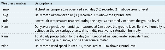
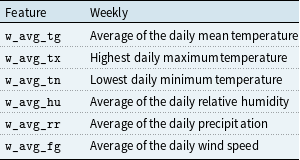
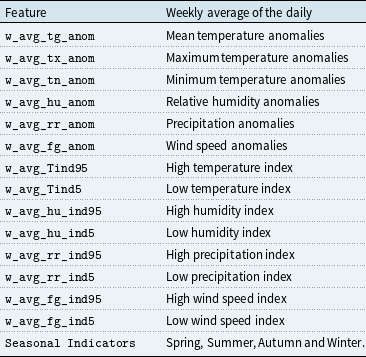
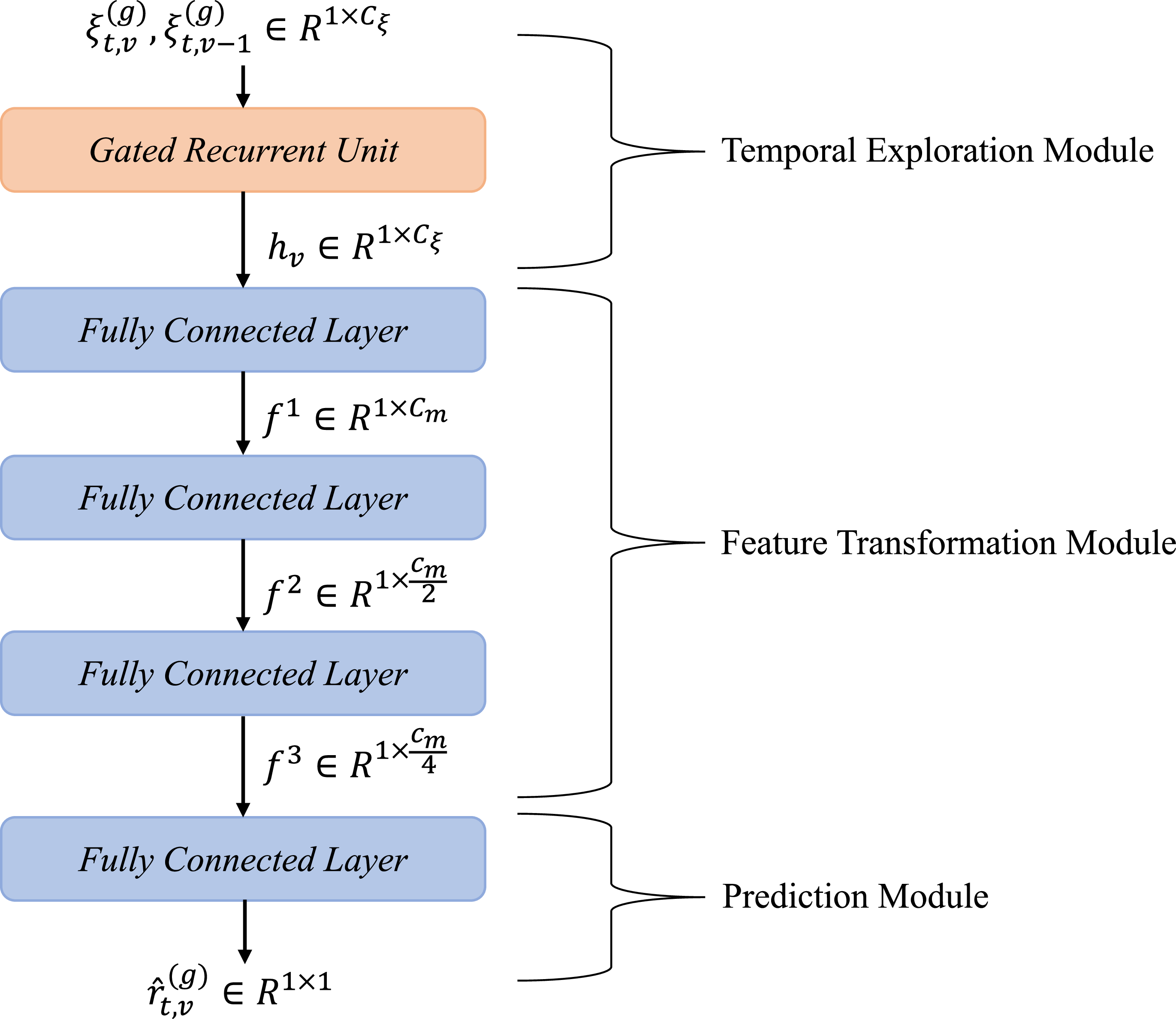
 ξt,v(g)
 ξt,v−1(g)
 hv
hv hv
hv f1
f1 f2
f2 f3
f3 r^t,v(g)
 Cξ
Cξ Cm
Cm R
R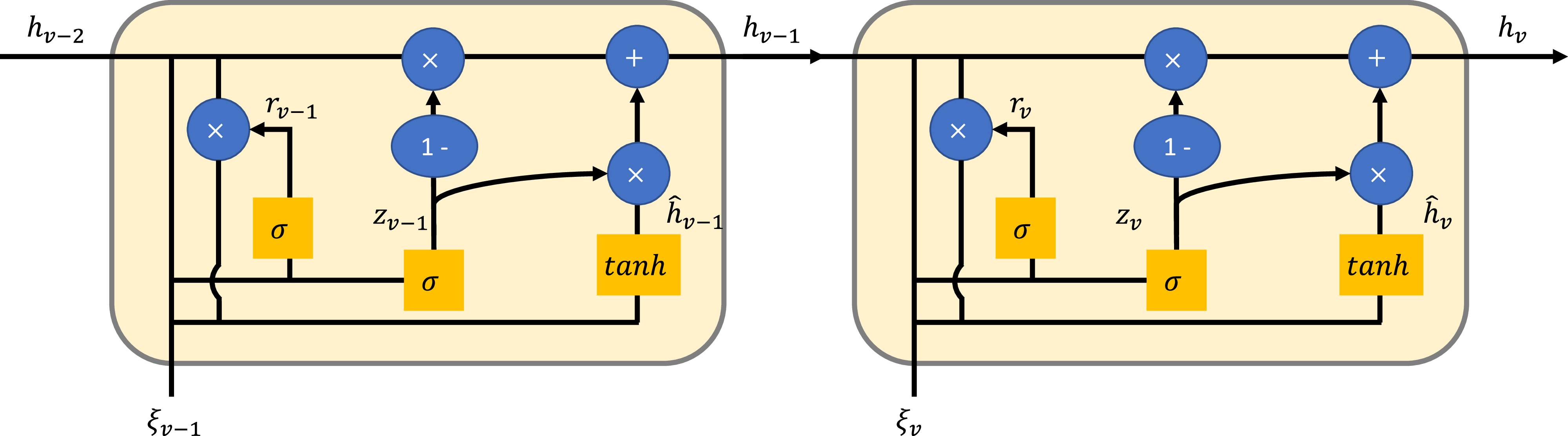
 ξv−1
ξv−1 ξv
ξv v
v ξv
ξv hv−1
hv−1 zv
zv rv
rv hv
hv h^v
h^v σ
σ tanh
tanh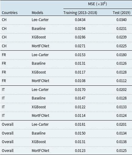
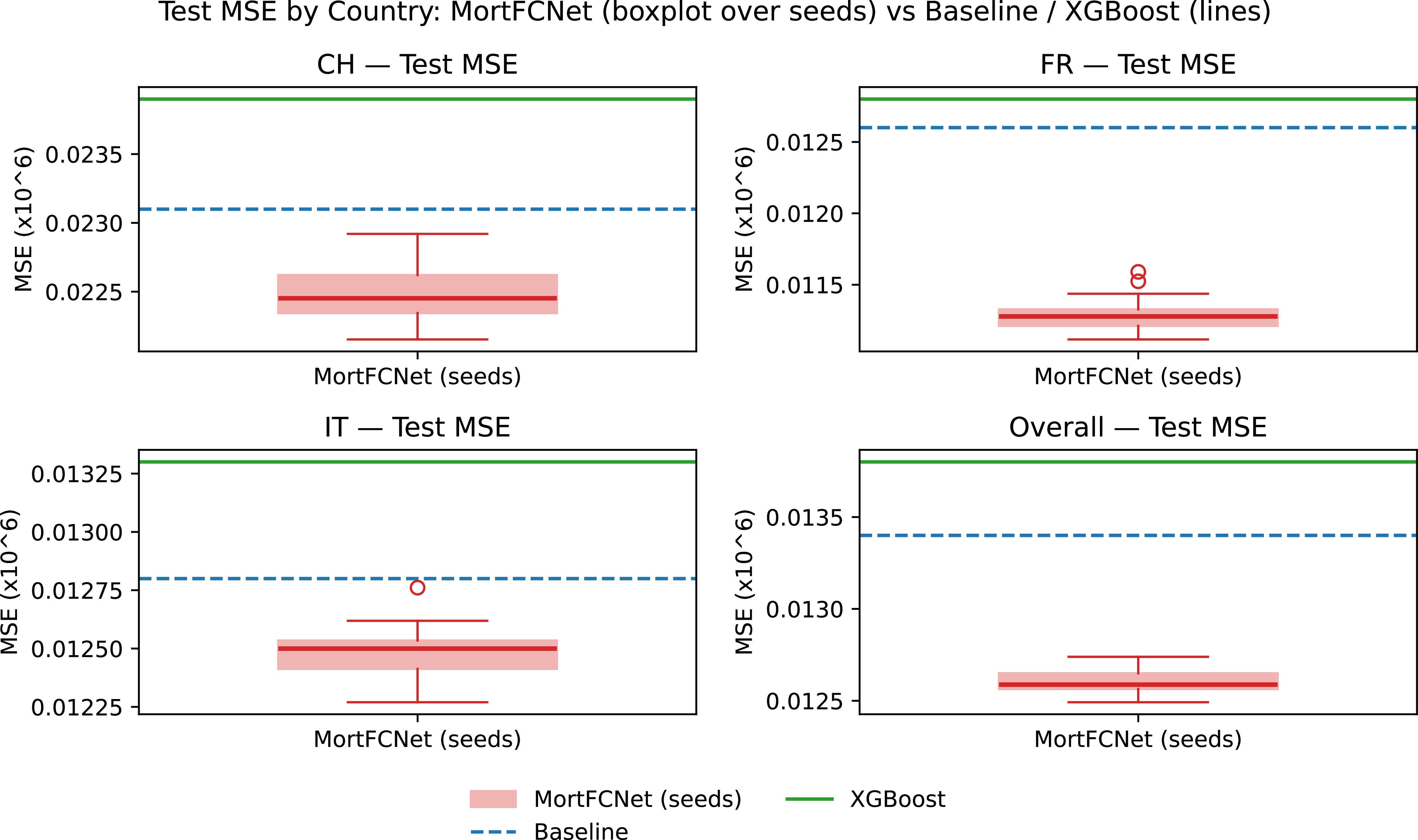


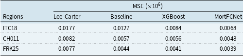


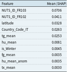
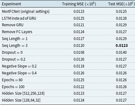
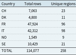
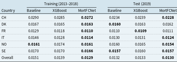
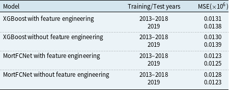

 Open access