Introduction

The evolution of glacier volume and area can be estimated by employing the volume–area scaling approach (Reference Bahr, Meier and PeckhamBahr and others, 1997) during surface mass-balance modelling (e.g. Reference Van de Wal and WildVan de Wal and Wild, 2001; Reference Radić, Hock and OerlemansRadić and Hock, 2007). If the studied glacier or ice cap is not in steady state, this method requires information on the initial surface area and ice volume to adjust the volume–area relation to the specific ice body (e.g. Reference Radić, Hock and OerlemansRadić and Hock, 2007). However, as absolute volumetric data on glaciers and ice caps are very rare, the applicability of volume–area scaling is limited. Data regarding glacier area are available much more readily.

We present a new method to calibrate the volume- area relation applied in volume- and area-change modelling on the basis of areal data only and no absolute volumetric data. This makes it possible to extend the use of volume–area scaling to less intensively studied glaciers.

To calibrate the volume–area relation, it is necessary to know the surface areas at different dates in combination with the surface topography at the first date. A surface mass-balance model extended to incorporate changing glacier area by using the volume–area scaling approach is repeatedly run over the calibration period. The volume–area relation implemented in the model is then changed until the calculated surface area evolution reaches the best possible approximation of observed glacier changes.

The method is applied to an outlet glacier of Gran Campo Nevado (GCN) ice cap in southernmost Chilean Patagonia, unofficially named Glaciar Noroeste (Fig. 1; Reference Schneider, Schnirch, Acuña, Casassa and KilianSchneider and others, 2007b). Its volume–area relation was calibrated using known glacier surface extents from 1984, 1986, 1998, 2002 and 2007. The derived volume–area relation was used to estimate future volume and area changes of Glaciar Noroeste by employing statistically downscaled general circulation model (GCM) data.

Fig. 1.

Location of Glaciar Noroeste and overview of its different glacier extents. Coordinates correspond to Universal Transverse Mercator (UTM) zone 18S. The contour interval is 100 m. Dark grey shading represents the sea.

Recent mass-balance and glacier change throughout Patagonia has been studied intensively during the past decade (e.g. Reference Casassa, Sepúlveda and SinclairCasassa and others, 2002; Reference Rivera, Acuña, Casassa and BownRivera and others, 2002; Reference Rignot, Rivera and CasassaRignot and others, 2003; Reference Stuefer, Rott and SkvarcaStuefer and others, 2007). Most of the studies focused on the Northern and Southern Patagonia Icefields. There are few studies of smaller glaciers of Patagonia and Tierra del Fuego. The regional focus is placed on Cordillera Darwin (e.g. Reference Porter and SantanaPorter and Santana, 2003), the Cordillera Fueguina Oriental on Tierra del Fuego (e.g. Reference Strelin and IturraspeStrelin and Iturraspe, 2007) and GCN ice cap in southernmost Patagonia (e.g. Reference Möller, Schneider and KilianMöller and others, 2007; Reference Schneider, Kilian and GlaserSchneider and others, 2007a,Reference Schneider, Schnirch, Acuña, Casassa and Kilianb; Reference Möller and SchneiderMöller and Schneider, 2008), which forms the largest Patagonian ice mass outside the Northern and Southern Patagonia Icefields (190.5 km² in 2007). However, to our knowledge, there is no reliable estimation of possible future changes in surface area or ice volume for Patagonian ice caps and glaciers. Hence, we aim not only at introducing a new methodology for glacier volume assessment, but also at presenting a contribution to the assessment of glacier change during the 21st century in Patagonia.

Data

The glacier outlines of Glaciar Noroeste used in this study (Fig. 1) were digitized from aerial photographs taken in 1942, 1984 and 1998, from Landsat Thematic Mapper images taken in 1986 and 2002 and from an Advanced Spaceborne Thermal Emission and Reflection Radiometer (ASTER) image acquired in 2007. Drainage basin boundaries correspond to glacier inventory data presented by Reference Schneider, Schnirch, Acuña, Casassa and KilianSchneider and others (2007b). The surface area of Glaciar Noroeste shows a continuous decline (Table 1).

Table 1.

Observed and modelled surface extents of Glaciar Noroeste

The glacier surface topography of Glaciar Noroeste is represented by a digital elevation model (DEM) based on topographic maps produced from 1984 airborne photographs (Reference Schneider, Schnirch, Acuña, Casassa and KilianSchneider and others, 2007b). Local reference data needed for statistical downscaling and set-up of the surface mass-balance model, which is based on the degree-day method, were provided by air-temperature and precipitation measurements from an automatic weather station (AWS) operated at Puerto Bahamondes about 7.5 km to the east of Glaciar Noroeste and 3.5 km from the eastern ice margin of GCN ice cap at 28 m a.s.l. (Reference Schneider, Glaser, Kilian, Santana, Butorovic and CasassaSchneider and others, 2003). Daily measurements of the AWS cover the period September 2000–August 2005.

The 1984–2099 monthly climate-data time series (Fig. 2) used as input for the modelling procedure were created from gridded surface air-temperature and precipitation data. For the period 1984–2006 we used monthly US National Centers for Environmental Prediction (NCEP)/US National Center for Atmospheric Research (NCAR) reanalysis data (resolution 2.5° × 2.5°; Reference KalnayKalnay and others, 1996) provided by the Climate Diagnostics Center, National Oceanic and Atmospheric Administration Cooperative Institute for Research in Environmental Sciences (NOAA-CIRES), Boulder, Colorado, USA (http://www.cdc.noaa.gov/). These data served as the basis for calibration of the volume–area relation (Equation (7)). Output from the third UK Meteorological Office Hadley Centre coupled ocean–atmosphere GCM (HadCM3) was used for the remaining period (2007–99) of the climate-data time series. The HadCM3 datasets (resolution 3.75° × 2.5°; J.A. Lowe, http://cera-www.dkrz.de/WDCC/ui/Compact.jsp?acronym=UKMO_HadCM3_SRESA2_1; J.A. Lowe, http://cera-www.dkrz.de/WDCC/ui/Compact.jsp?acronym=UKMO_HadCM3_SRESB1_1) represent SRES (Special Report on Emissions Scenarios) scenarios A2 and B1 of the Intergovernmental Panel on Climate Change (IPCC) Fourth Assessment Report (Reference SolomonSolomon and others, 2007). Data were provided by the Hadley Centre. All gridded climate data were reduced to subsets of four gridpoints located near GCN ice cap. Data were statistically downscaled according to a combined method (Reference Möller and SchneiderMöller and Schneider, 2008) employing ‘local scaling’ (Reference Widmann, Bretherton and SalathéWidmann and others, 2003; Reference SalathéSalathé, 2005) for adjustment of the annual cycles to local conditions at GCN ice cap and multiple linear regression analysis for creating best-fit combinations of the four gridpoints. NCEP/NCAR reanalysis and HadCM3 A2 time series are the same as in Reference Möller and SchneiderMöller and Schneider (2008), while the HadCM3 B1 time series were created accordingly. The similarity between the downscaled scenarios A2 and B1 is a result of the shift of the different initial air-temperature levels of both scenarios to local conditions at GCN ice cap during the downscaling procedure. As the long-term trends of both scenarios show only small differences, this leads to comparable future time series. A quality assessment of the downscaling procedure based on data from AWS Puerto Bahamondes is presented in Table 2. Results indicate a good performance of the downscaling procedure, with the explained variances of all surface air-temperature time series amounting to at least 84%. Even the synthetic HadCM3 precipitation time series account for explained variances of up to 33% after the downscaling. Hence, all climate data used are considered an appropriate basis for future glacier evolution modelling.

Fig. 2.

Downscaled air-temperature and precipitation time series for 1984–2099. The period 1984–2006 is covered by NCEP/NCAR reanalysis data, the period 2007–99 by different HadCM3 data.

Table 2.

Performance of the combined downscaling procedure of air-temperature and precipitation data. Measurements at the AWS during September 2001–August 2005 serve for comparison. Significance levels according to Student’s t test refer to linear correlations between downscaled and measured data

Methods

Surface mass-balance model

The modelling of glacier volume and area changes builds upon an altered version of the surface mass-balance model described by Reference Möller, Schneider and KilianMöller and others (2007). Within the model, ablation is calculated using the degree-day method (e.g. Reference BraithwaiteBraithwaite, 1981; Reference OhmuraOhmura, 2001; Reference HockHock, 2003) and accumulation results directly from altitude-dependent sums of solid precipitation. The computation of ablation, a, at a specific altitude, z, is based on the positive degree-day sum, DD ⁺ of the considered month, i, and an empirically derived degree-day factor, f. It is calculated as

(1)

Following Reference BraithwaiteBraithwaite (1984) and Reference Marshall and KnightMarshall (2006), the calculation of is based upon the integral over the positive interval of the probability density function of air temperature (PDF _T ) of the respective month, p_i(T_z ); (Fig. 3; Equation (4)):

(2)

D_i is the number of days of the respective month. is the mean of all positive monthly air temperatures. It is calculated by solving

(3)

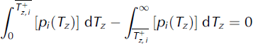
for (Fig. 3). The employed PDF _T is the normal distribution

(4)

with σ representing the standard deviation of air temperature and the mean monthly air temperature.

Fig. 3.

PDF _T for GCN ice cap for any given mean monthly air temperature, . Grey areas mark the cumulated probability of positive air temperature. subdivides the cumulated probability of positive air temperature into parts of equal size indicated by light grey and dark grey areas. Standard deviations of the PDF _T are based on measurements carried out at AWS Puerto Bahamondes between September 2000 and August 2005.

The accumulation, c, at a specific altitude, z, during a specific month, i, likewise depends on the PDF _T (Equation (4)). It is calculated as the proportion of solid precipitation of the monthly precipitation sum (P_z , _i ) according to Reference Marshall and KnightMarshall (2006) as

(5)

It thus features the probability of negative air temperatures as scaling factor, so that solid precipitation is limited to air temperatures below 0°C.

To obtain the specific mass balance at each altitude, ablation is subtracted from accumulation. To convert the specific mass balance into volume changes, the model is extended to a surface mass-balance model according to Reference Braithwaite and ZhangBraithwaite and Zhang (2000) on the basis of the DEM representing the glacier surface, A. Volume changes, ΔV, are calculated by integrating the specific mass balance over all altitudes:

(6)

with ρ _Ice, the density of glacier ice, set to 0.9 (Reference PatersonPaterson, 1994; Reference Möller, Schneider and KilianMöller and others, 2007). At this stage (Equations (1–6)) the surface mass-balance model architecture lacks any dynamic adjustment of the glacier surface area to volume changes.

Volume–area scaling

According to Reference Bahr, Meier and PeckhamBahr and others (1997), the volume, V, of any glacier or ice cap is related to its surface area, A, by a simple power-law equation based on a dimensionless scaling exponent, γ, that depends on glacier type:

It is extended by a scaling coefficient, sc, to account for any glacier, either in steady state or not (Reference Van de Wal and WildVan de Wal and Wild, 2001; Reference Radić, Hock and OerlemansRadić and Hock, 2007):

(7)

In steady state, sc = 1. Otherwise, sc has to be obtained for each glacier individually. This can be done either by calculating it from the glacier’s known initial surface area and ice volume (Reference Radić, Hock and OerlemansRadic’ and Hock, 2007) or by applying the method presented here.

Area- and volume-change modelling

Based on the volume–area relation, and according to a method outlined in Reference Van de Wal and WildVan de Wal and Wild (2001) and Reference Radić, Hock and OerlemansRadić and Hock (2007), the surface mass-balance model is augmented by an area- and volume-change model. It employs the volume–area scaling equation (Equation (7)) for continuous adjustment of glacier surface area to computed volume changes. During model runs, the monthly changes of glacier volume calculated by the area- and volume-change model, ΔV, are summed at the end of each year, y. This sum is then added to the existing glacier volume, V, in order to calculate a new glacier area, A, for the following year according to

(8)

For areas smaller than the initial glacier area, the lower ice margins are moved upwards until the remaining surface extent equals the previously calculated new glacier area. This method is similar to an approach used by Reference Paul, Maisch, Rothenbühler, Hoelzle and HaeberliPaul and others (2007) who carried out glacier area modelling depending on varying accumulation-area ratios. During model runs, the glacier area is reduced by cutting off pixels of the DEM in order of increasing altitude. Calculation of ΔV for the particular year is then based on the reduced DEM. In case of positive mass balance, the enlargement of the glacier area is performed by extending it to formerly ice-covered regions (Fig. 1). During model runs, this expansion of glacier area is done by adding pixels to the DEM in order of decreasing altitude.

Model Calibration

We introduce a new method to calibrate the volume–area relation (Equation (7)) of a specific glacier that is not in steady state. The basic idea is to run the area- and volume-change model from a known initial state over a certain period featuring one or, ideally, more known surface extents of the respective ice body. Referring to Reference Bahr, Meier and PeckhamBahr and others (1997), we assume (see below) a fixed value for the scaling exponent, γ (Equation (7)), and during calibration runs we alter the factor sc iteratively to seek the best fit between modelled glacier area change and observed glacier-extent records by minimizing the root-mean-square (RMS) difference.

For the volume–area scaling equation (Equation (7)), Reference Bahr, Meier and PeckhamBahr and others (1997) obtained a dimensionless scaling exponent of γ = 1.375 for valley glaciers. They also outline that other studies resulted in slightly different scaling exponents, which is in good agreement with findings by Reference PatersonPaterson (1972), Reference Chen and OhmuraChen and Ohmura (1990) and Reference Radić, Hock and OerlemansRadić and others (2007). Considerations by Reference Van de Wal and WildVan de Wal and Wild (2001) suggest an error range for γ of ±0.125. Accordingly, in this study, γ for Glaciar Noroeste is assumed to be 1.375 ± 0.125, which combines the scaling exponent given by Reference Bahr, Meier and PeckhamBahr and others (1997) and the error range of Reference Van de Wal and WildVan de Wal and Wild (2001).

The 1984 glacier surface extent (Fig. 1) and topography were used as initial conditions for the area- and volume-change model runs. The remaining boundary and starting conditions of the model were chosen according to Reference Möller, Schneider and KilianMöller and others (2007) and Reference Schneider, Kilian and GlaserSchneider and others (2007a). The degree-day factors (Equation (1)) of the surface mass-balance model were set to f = 7.0 mm w.e. K⁻¹ d⁻¹ for ice surface and f = 3.5 mm w.e. K⁻¹ d⁻¹ for snow surface. An initial snow-cover pattern ranging between 0 mm w.e. thickness below 300 m a.s.l. and 500 mm w.e. thickness above 700 m a.s.l. was included. A further increase of snow depth above this altitude has no influence on model results. Therefore, it is kept constant in favour of model simplicity. Air-temperature and precipitation lapse rates were set to 0.63 K (100 m)⁻¹ and 5%(100 m)⁻¹ respectively, as estimated from different AWS measurements documented by Reference Schneider, Glaser, Kilian, Santana, Butorovic and CasassaSchneider and others (2003). The standard deviation of mean daily air temperature at GCN ice cap (σ = 3.5°C) required for set-up of the PDF _T (Equation (4)) is calculated from the mean daily temperatures of the AWS (September 2000–August 2005).

The known glacier surface extents of 1986, 1998, 2002 and 2007 serve as benchmarks for the best-fit calibration procedure. Model runs are driven by downscaled NCEP/NCAR reanalysis data of the period 1984–2006 (Fig. 2).

Results yield sc = 0.311 m ^3−2γ, and Equation (7) thus becomes

(9)

for Glaciar Noroeste. Table 1 presents the modelled and observed glacier extents, providing an overview of the model performance, and showing that modelled glacier changes provide a reasonable estimate of the surface extents observed within the calibration period. The RMS error between observed and modelled values amounts to just 0.24 km², indicating a good overall reliability of the area-and volume-change model.

Error Assessment

For assessment of the error range of both area- and volume-change modelling, three different sources of errors have to be considered. The set is formed by (1) the RMS difference of the best-fit calibration procedure; (2) an additional error range resulting from the ±0.125 uncertainty of the scaling exponent of the volume–area relation itself; and (3) possible inaccuracies of the degree-day model calibration.

The RMS error of the best-fit calibration procedure was calculated using observed and modelled extents of Glaciar Noroeste in 1986, 1998, 2002 and 2007 (Table 1). It amounts to ±0.24 km² for area-change modelling, E_{A , 1}, and is assumed to be constant in time. The associated error range in volume-change modelling, E_{V , 1,} is thus calculated to be ±0.04 km³ according to the volume–area relation (Equation (9)).

For assessment of the error resulting from the ±0.125 uncertainty of the scaling exponent of the volume–area relation (Equation (9)), the area and volume changes of Glaciar Noroeste during the 21st century were computed repeatedly using not only Equation (9) for the area- and volume-change model but also Equation (7) calibrated for γ = 1.25 and γ = 1.5. The differences between the resulting three modelled area-change time series show clearly progressive characteristics. Maximum differences are reached in 2099 and amount to ±0.22 km² (B1) and ±0.24 km² (A2). The deviations of volume-change modelling prove to vary only slightly with time. Starting with a value of ±1.21 km³ in 1984, they show an increase to slightly higher maximum values during the first three decades of the 21st century. Afterwards, deviations drop continuously until 2099. Minimum values are reached at ±1.19 km³ (B1) and ±1.18 km³ (A2) respectively. The corresponding error ranges result from the maximal deviations of each year, E(y) _{A , 2} and E(y) _{V , 2}.

The impacts of calibration inaccuracies of the degree-day model, i.e. of the degree-day factors, were also analysed by performing additional area- and volume-change model runs. For error assessment the degree-day factors, f _ice = 7.0 mm w.e. K⁻¹ d⁻¹ and f _snow = 3.5 mm w.e. K⁻¹ d⁻¹, were varied by ±1.0 and ±0.5 mm K⁻¹ d⁻¹ respectively. Results of area-change modelling yield a continuous but decreasing progression of deviations throughout the modelling period. Maximum values are reached in 2099 and amount to ±3.1 km² (B1) and ±3.2 km² (A2). The uncertainty in the modelled volume-change time series shows similar characteristics, with deviations of up to ±0.9 km³ (B1 and A2). Maximum deviations of each respective year are taken as error ranges E(y) _{A , 3} and E(y) _{V , 3}.

The total error ranges of the area- (Equation (10a)) and volume-change (Equation (10b)) time series can be described by

(10a)

and

(10b)

The total error ranges of the area-change time series show a continuous increase with time. They reach maximum uncertainties of ±3.2 km² (B1 and A2) in 2099 (Fig. 4). This corresponds to values of not more than ±9% for any specific year. Regarding the error ranges of the volume-change time series, only a slight increase with time is evident. Uncertainties increase continuously from ±1.2 km³ in 1984 to ±1.5 km³ (B1 and A2) in 2099 (Fig. 5). Thus, they increase from consistent values of ±9% in 1984 to 20% (B1) and 21% (A2) in 2099.

Fig. 4.

Evolution of the surface area extent of Glaciar Noroeste for the period 1984–2099.

Fig. 5.

Volume-change evolution of Glaciar Noroeste for the period 1984–2099.

The accuracy of modelled area changes proved to be highly reliable. This is documented by an RMS error of just 0.24 km². Moreover, the maximum deviation between modelled and observed glacier areas throughout the calibration period (i.e. the years 1986, 1998, 2002 and 2007) amounts to no more than 0.3 km², i.e. <0.5%.

Results and Discussion

Future glacier evolution

The results of modelling future ice evolution yield values of probable glacier surface area reduction by 2099 ranging from 18.9 km² (B1) to 19.4 km² (A2). This results in the surface area of Glaciar Noroeste being reduced to 34.9 ± 3.2 km² at the end of the 21st century for A2 (Fig. 4). In scenario B1, Glaciar Noroeste shrinks to 35.4 ± 3.2 km² (Fig. 4). This loss in area corresponds to between 35% (B1) and 36% (A2) when compared with the initial surface area in 1984. Volumetric results (Fig. 5) reveal a probable ice volume loss ranging from 5.9 km³ (B1) to 6.1 km³ (A2). The calibrated initial ice volume of 13.4 ± 1.2 km³ is estimated to decrease to 7.4 ± 1.5 km³ (B1) and 7.3 ± 1.5 km³ (A2). This implies a loss of ice volume of >40% in both cases.

The associated recession of the lower ice margins was estimated to altitudes of 539 ± 37 m a.s.l. (B1) and 546 ± 40 m a.s.l. (A2). Figure 6 shows the different estimates of surface extent of Glaciar Noroeste in 2099. The modelling procedure does not account for lowering of the glacier surface. The potential elevation feedback (e.g. Reference Raymond, Neumann, Rignot, Echelmeyer, Rivera and CasassaRaymond and others, 2005) resulting in altered ablation and accumulation amounts is thus neither considered nor quantified. The resulting additional error range of unknown magnitude due to feedback mechanisms should not be ignored when the presented area and volume changes are interpreted. Nevertheless, the small differences between the B1 and A2 time series in either case suggest only a weak dependency of Glaciar Noroeste on the intensity of oncoming climate change.

Fig. 6.

Estimated extents of Glaciar Noroeste in 2099 resulting from climate forcing according to IPCC SRES scenarios B1 (left) and A2 (right). Coordinates correspond to UTM zone 18S. The contour interval is 100 m. Dark grey shading represents the sea. Given uncertainty ranges correspond to the results of Equation (10a).

Conclusion

We have presented a new method to calibrate the volume–area relation of a specific glacier or ice cap without requiring information regarding absolute ice volume. The only data needed for the calibration process are a DEM representing the terrain at the beginning of a calibration period and several known glacier surface extents.

Calibration results combined with error assessment yield a good model performance. Area changes prove to be modelled with high accuracy within the period 1984–2007. Initial ice volume is estimated with a precision of ±10%. However, this finding is not derived from ice volume observations but is merely based on error propagation. Our method has high potential for estimating the volume of glaciers. The area- and volume-change model also proved to be a useful and reliable means of modelling future glacier evolution. Due to its low requirements regarding input data, the method is especially valuable for studies on remote and thus less intensively studied regions.

The area- and volume-change model was calibrated and tested for Glaciar Noroeste, an outlet glacier of GCN ice cap. The range of future volume and area changes of Glaciar Noroeste until 2099 was estimated. Model results yield a decline of the glaciated area of Glaciar Nooroeste from 54.3 km² in 1984 to between 35.4 ± 3.2 km² (B1) and 34.9 ± 3.2 km² (A2) at the end of the 21st century (Fig. 4). This change will probably be accompanied by a recession of the lower ice margins to altitudes between 539 ± 3 7 m a.s.l. (B1) and 546 ± 40 m a.s.l. (A2) when assuming a hypsometrically consistent retreat in the lowermost glacier regions (Fig. 6). The associated loss of ice volume (Fig. 5) was estimated to range between 5.9 km³ (B1) and 6.1 km³ (A2). The small difference in probable future glacier changes of Glaciar Noroeste suggests a weak dependency on the intensity of oncoming climate change, which in this region is dominated by a temperature increase of <2°C in both B1 and A2 scenarios by the end of the century, with insignificant change in precipitation (Fig. 2).