


1. INTRODUCTION
Hydraulic roughness is a model parameterization that accounts for head losses occurring over unit channel length scale as friction and turbulence dissipate gravitational potential energy of flowing water to heat. Because head losses generate heat, they play a critical role in regulating enlargement of subglacial conduits (Shreve, Reference Shreve1972). Conduits in turn regulate subglacial water pressure and link hydrology and sliding (Bindschadler, Reference Bindschadler1983). Proper parameterization of hydraulic roughness in subglacial hydrological models is therefore critical to correctly simulate timescales of conduit enlargement by melt and the spatial distribution of subglacial water pressure that controls sliding (Gulley and others, Reference Gulley2014). While there has been a proliferation of models of subglacial conduit hydrology, little is known about magnitudes of hydraulic roughness in actual subglacial conduits, or how roughness evolves in response to conduit enlargement and creep closure. This is due to the paucity of direct observations of subglacial conduits and the features in them that contribute to hydraulic roughness.
The importance of head losses and hydraulic roughness in subglacial hydrological systems can be demonstrated by comparing an idealized example of a glacier hydrological system where water is both irrotational and inviscid with actual glacier hydrological systems. The Bernoulli equation expresses conservation of total energy of a parcel of an inviscid and incompressible fluid moving in steady state (Munson and others, Reference Munson, Young, Okiishi and Heubsch2009),
 $$\left( {\displaystyle{\,p \over \gamma} + \displaystyle{{v^2} \over {2 g}} + z} \right) = C,$$
with p pressure, γ the specific weight ( $\rho g$), v velocity, g gravitational acceleration and z elevation. Eqn (1) states that the sum of the pressure head (p/γ), the velocity head (v 2/2g) and the elevation head (z) remain constant (C) along a streamline. Without viscous dissipation, Eqn (1) indicates that 100% of the gravitational potential energy drop would convert to kinetic energy as water flows into a moulin, passes through a subglacial conduit and exits the glacier, resulting in unrealistically high exit velocities of water from subglacial conduits (Liestøl, Reference Liestøl1956). For a glacier that is 100 m thick and where water has backed up in moulins to the ice surface elevation, discharge velocity at the terminus would have to reach 44 m s–1 if there were no head losses. However, water actually exits glaciers in proglacial streams with average velocities ranging from 1 to 10 m s–1 (Chikita and others, Reference Chikita, Kaminaga, Kudo, Wada and Kim2010) and likely lower velocities for submarine discharges (e.g. Mankoff and others, Reference Mankoff2016). The difference between the exit velocities of water from an idealized frictionless system and from actual glaciers indicates that nearly all of the gravitational potential energy available at the surface is dissipated under the glacier.
Hydraulic roughness is commonly parameterized in hydrological models, including glacier drainage models, using the Manning roughness coefficient n, Darcy–Weisbach friction factor f, or Nikuradse roughness k (e.g. Nikuradse, Reference Nikuradse1950; Röthlisberger, Reference Röthlisberger1972; Nye, Reference Nye1976; Hewitt, Reference Hewitt2011; Gulley and others, Reference Gulley2014; Perol and others, Reference Perol, Rice, Platt and Suckale2015). Each of the variables n, f and k has been empirically related to conduit features, such as rocks that protrude into flowing water and contribute to head losses. The size of these protrusions exerts an important control on discharge and head loss, with the impact of those objects on flow decreasing with increasing flow depth (Smart and others, Reference Smart, Duncan and Walsh2002). For conduits filled with water, flow depth is determined by the hydraulic diameter and cross-sectional area. The relationship between the size of roughness elements protruding into the flow and the pipe-full equivalent depth of that flow, is termed relative roughness and defined as,
 $$r_{\rm r} = \displaystyle{r \over {D_{\rm H}}}. $$
In Eqn (2), D H is the hydraulic diameter, defined as
 $$D_{\rm H} = \displaystyle{{4A} \over P},$$
where A is the cross-sectional area and P the perimeter length, for a full pipe. The r variable in Eqn (2) is some measure of the roughness of the bed. This can be the standard deviation of a digital surface model (DSM) (i.e. r = σ z as in Smart and others, Reference Smart, Aberle, Duncan and Walsh2004), a given percentile of the intermediate (b) axis of the rocks (e.g. r = d 50 or r = d 84; Wolman, Reference Wolman1954; Limerinos, Reference Limerinos1970), or some other measure (e.g. Nikora and others, Reference Nikora, Goring and Biggs1998; Smart and others, Reference Smart, Duncan and Walsh2002, Reference Smart, Aberle, Duncan and Walsh2004; Nikora and Walsh, Reference Nikora and Walsh2004).
Manning roughness coefficients and Darcy–Weisbach friction factors can only be directly related to relative roughness where the latter is <5% (Moody, Reference Moody1944). Because relative roughness is a function of r, which is not strictly defined, in practice it is better not to approach the 5% limit. Relative roughness values  ${\rm \ll} 5\% $ are common in the deep rivers, storm drains, man-made channels and pipes for which the Darcy–Weisbach and Manning equations were developed. When relative roughness values exceed ~5%, however, the size of roughness elements becomes large relative to water flow depth. As a result, large roughness elements generate chaotic disruptions in water flow that depend on the size and location of individual roughness elements; consequently, relative roughness cannot be statistically related to head loss. Furthermore, estimates of roughness for Manning's equation were developed for open channel flow. The Darcy–Weisbach equation was derived in pipe-full settings, but under conditions simplified to a straight circular pipe with uniform roughness and cross section (Powell, Reference Powell2014). Applying these equations to a subglacial conduit with high and variable relative roughness and changing cross section and direction, may be outside of their empirically derived bounds (Gulley and others, Reference Gulley2014). Another approach is to perform an inverse estimate of hydraulic roughness from direct measurement of head loss along a flow path (Jarrett, Reference Jarrett1984) but discharge, pressure gradient and hydraulic diameter have to be known at two or more points along a flow path. This hydraulic roughness value can be used to parameterize hydrological models but it is rarely directly attributed to physical features of streams or conduits. Connecting specific physical objects in a pipe to observed head loss is difficult because the head-loss calculations necessarily treat the system between the two head measurement points as a black box. Such inverse calculations ascribe all head losses to the effects of friction, including the ones that are associated with changes in overall conduit geometry (e.g. diameter changes, turns, large obstacles) rather than wall roughness.
Measurements of relative roughness and hydraulic roughness are difficult to obtain in subglacial conduits because the glacier generally prevents access for direct measurement. In addition, the size of conduits and of bed materials (i.e. rocks) that contribute to roughness are below the resolution of indirect measurement techniques such as geophysical instrumentation (e.g. Jezek and others, Reference Jezek, Wu, Paden and Leuschen2013).
There seems to be little hope of relating hydraulic roughness coefficients used in subglacial hydrological models to the physical features of actual subglacial conduits until conduit diameters exceed one to several meters (Gulley and others, Reference Gulley2014). However, parameterization of hydraulic roughness in larger-diameter subglacial conduits can be improved if realistic sizes of roughness elements are known. Currently, few quantitative constraints on roughness element size distributions exist. To address this knowledge gap, our paper presents the first high-resolution survey of roughness elements in a subglacial conduit. Data were acquired through in-situ exploration of a subglacial conduit under Hansbreen, a polythermal glacier in Svalbard, Norway. The conduit was mapped at the end of the 2012 melt season when it was large and minimal water inputs permitted access and direct observation. We used two complementary techniques to quantify elements contributing to conduit roughness: structure-from-motion (SfM) and hand measurements of rock sizes. We use this information to characterize conduit bed roughness heights, alignment of roughness elements, conduit hydraulic diameter and how relative roughness changes as a conduit grows.
1.1. Field site
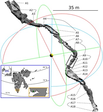
In October 2012 we accessed and mapped a subglacial conduit beneath Hansbreen near 77.03°N, 15.55°E. The conduit extended from the base of a relict hydrofracture located in the wall of an ice marginal lake basin at the eastern edge of the Vesletuva nunatak. A prominent notch in the lake basin indicated that the basin had filled and melting occurred at the water line. We do not, however, know the date of lake drainage, nor do we have any constraints on the volume of water flowing into the conduit during the melt season after lake drainage. In 2015 and 2016, however, high-resolution DigitalGlobe WorldView-2 imagery shows that the lake drained between 1 and 10 July and had a surface area of ~16 000 m2. We estimate an average depth of ~5–10 m and therefore a volume of 80 000–160 000 m3. This particular conduit has been accessed in multiple years and the lengths of the accessible portions of the conduit have changed each year (Gulley and others, Reference Gulley2012). In 2012, the total conduit length was ~600 m. We made high spatial resolution surveys of ~125 m of the conduit beneath a maximum ice thickness of ~100 m (Fig. 1). We focus our analysis on a 9 m long subset, located near the middle of that segment (Figs 2–4).
3-D model of subglacial conduit from SfM. Dark gray is exterior of conduit and light gray is interior where the roof is ‘open’. The conduit roof was not the primary target, and is therefore not captured in all segments. Labels An and dashed lines demarcate approximate locations of GCPs collected with the standard speleological method. Curved solid lines connecting GCPs show where hand-count data were collected. Black rectangle near A9–A11 is examined in detail in subsequent figures. Inset map shows location of Svalbard and the conduit.

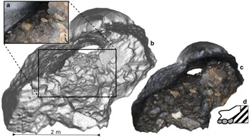
Detailed 3-D model of a subglacial conduit. Observer is near GCP A9 and looking down-conduit toward A10 (distal). (a) Example photograph input to SfM software used to produce (b) meshed grid and (c) photo-realistic model. (d) Previous description of this segment from Gulley and others (Reference Gulley2012), showing schematic of boulders on floor and rocky (striped) wall.

2. DATA COLLECTION AND PROCESSING
We collected data using (1) standard cave survey methods (Gulley, Reference Gulley2009), and (2) photographs combined with SfM (James and Robson, Reference James and Robson2012; Westoby and others, Reference Westoby, Brasington, Glasser, Hambrey and Reynolds2012; Fonstad and others, Reference Fonstad, Dietrich, Courville, Jensen and Carbonneau2013) algorithms to make a three-dimensional (3-D) model of the conduit. Additional data were also collected with the Kinect, a Microsoft XBox video game 3-D camera that can be used as a portable LiDAR-like sensor (Mankoff and Russo, Reference Mankoff and Russo2013). The Kinect is not used in depth in the analysis here, due to large-scale scene reconstruction issues, but is used as a high-resolution (mm-scale) visual of rocks on the conduit floor.
Standard cave survey data were collected at 18 ground control points (GCPs) along ~125 m of conduit and statistical results are presented for the entire conduit length. Photographs for SfM were collected along the entire conduit. A low-resolution SfM model was generated for the entire conduit and is used for the overview Figure 1. A high-resolution SfM segment near the middle of the conduit is analyzed in more detail.
2.1. Conduit mapping
2.1.1. Standard method
Standard cave survey methods (Gulley, Reference Gulley2009) were used to record the maximum conduit width and height at 18 GCPs along 125 m of subglacial conduit, and the orientation between GCPs (labeled A1–A18 in Table 1 and Fig. 1). The location of each GCP was converted to WGS84 latitude, longitude and altitude above sea level based on the approximate position of the top of the moulin, and the position and orientation of each downstream GCP relative to its upstream neighbor.
Data collected by the standard speleological technique (Gulley, Reference Gulley2009)

Distance (d), horizontal angle (α) and elevation angle (θ) are from the GCP on the reported line to the next GCP (on the line below). Width and height describe the cross section at each GCP.
2.1.2. Structure-from-motion
We used SfM to produce a digital 3-D model of the subglacial conduit. Approximately 1200 photographs were taken of the interior of the conduit for the SfM algorithm, which derives 3-D models from photographs. SfM works best with a lot of photographic overlap, heterogeneous scenery and dense GCPs. We had a highly homogeneous surface and few GCPs, and therefore difficulty producing a high quality DSM over the entire conduit length. We grouped photographs into subsets where each subset contained three sequential GCPs, and identified the GCPs in photos when possible, because three GCPs are needed to orient a model in world coordinates. We produced geo-referenced 3-D model segments using Agisoft PhotoScan Pro and then combined segments for the final low-resolution model with ~50 cm resolution in x, y and z. Near the middle of the conduit near station A10, a higher resolution reconstruction succeeded due to the heterogeneous rock wall and more photographs (Fig. 2).
2.2. Conduit roughness measurements
2.2.1. Rock b-axis measurements
We used hand-measurements of the intermediate axis (b-axis) of 100 rocks between seven stations in the conduit (curved lines connecting GCPs in Fig. 1) to define the frequency distribution of roughness heights (Wolman, Reference Wolman1954). Rocks were chosen by one participant crawling and pointing randomly with eyes closed. Another participant then measured the b-axis of the selected rock with a tape measure.
2.2.2. Structure-from-motion
A ~9 m long conduit segment containing the high resolution reconstruction is detailed near GCP A10 (boxed region in Fig. 1). This section corresponds to the schematic labeled A8 in Figure 3a of Gulley and others (Reference Gulley2012), with that schematic reproduced here for comparison (Fig. 2d).

When discussing the 9 m sub-section, we rotate it in 3-D space so that x is along-conduit, y is across-conduit and z is perpendicular to the floor. We then grid only the SfM data points onto a 1 cm grid using the points2grid software (v 1.3.0, Crosby and others (Reference Crosby2011)). Our study focuses on the floor, with the exception of Figure 4a, because the data collection focused on the floor, and the ice roof roughness heights are of order of magnitude less than the floor roughness element heights, and therefore likely to meet the <5% roughness criterion.
Plan view of (a) conduit roof, (b) conduit floor z and floor decomposed into its (c) smoother DSM z s and (d) roughness elements z r (z = z s + z r). Both grayscale shading and contours show elevation above the local z = 0 level, set to the floor minimum in this segment. All values are in m, contour lines are at 10 cm intervals, and for (d), a residual product, the black contour line demarcates 0, solid white +10 cm and dashed white −10 cm. Sample cross section shown in Figure 5 is at the 4 m along-conduit mark. White circle in (b) marks station A10.

2.2.3. Kinect
We used the Kinect to capture small-scale (mm–cm) roughness heights of the rocky floor of the conduit. We scanned ~125 m of the conduit length and captured almost all segments of the floor from a distance of ~1.5 m resulting in ~1 mm resolution in x, y and z. We collected the data following the methods described by Mankoff and Russo (Reference Mankoff and Russo2013) and then used KinFu Large Scale (KFLS, Rusu and Cousins (Reference Rusu and Cousins2011)) to combine individual frames into a larger coherent model. We successfully reconstructed the segment around GCP A10, which overlaps with some of the dense SfM data. Data collection issues prevented reconstruction of other regions, but improved algorithms (Whelan and others, Reference Whelan2012) and better field hardware have overcome these issues in later years. Consequently, Kinect data are only used to provide a visual representation of the rocky floor and to show angularity of the rocks (Fig. 3).
2.3. Calculation of roughness height from DSMs
We use the term ‘roughness’ to describe the protrusions (pebbles, rocks) on the conduit floor. However, the distinction between a roughness element and the floor is not well defined, because the elevation of the floor changes throughout the conduit. DSMs are commonly decomposed into the mean elevation trend and the roughness elements by plane fitting or other low-pass filter methods (e.g. Smart and others, Reference Smart, Duncan and Walsh2002). In this work we use a 30 cm moving-window Gaussian filter over the DSM z (Fig. 4b) to define the conduit floor surface, z s (Fig. 4c) and then define the roughness elements as z r = z − z s (Fig. 4d). A sample cross section showing these different surfaces is shown in Figures 5a, b. The 30 cm size comes from an iterative application of the structure function analysis (see Appendix B), but results are not sensitive to this number (see Appendix C). We iteratively applied the structure function with increasingly large window sizes until the horizontal scales from that analysis were less than the window size.
Sample cross section (4 m into the high-resolution segment) showing (a) roof and floor z, (b) roof and floor decomposed into floor surface z s and floor roughness z r, and (c) three steps from the geometric growth model at this location. Braces at bottom show the width of the z r surface used for calculating the σ z standard deviation at each of the steps.

Probabilistic roughness heights are commonly computed from the standard deviation or a percentile of the b-axis measurements from a sample. We report the 50th (d 50) and 84th (d 84) percentile and standard deviation (σ b) of the diameter of the b axis from hand measurements (Wolman, Reference Wolman1954), and the d 50, d 84 and standard deviation (σ z) of the z r DSM (Smart and others, Reference Smart, Aberle, Duncan and Walsh2004) (Table 2). Because roughness is not strictly defined (Smith, Reference Smith2014), we report multiple values in some locations (Tables 2, 3). However, when performing the numeric analysis which uses the DSM, we use the  $\sigma _z = 0.07 {\rm m}$ from the SfM data. This is the smallest roughness size from our calculations, which means both roughness size and relative roughness values reported here can be considered a lower bound.
Measurements of roughness near GCP A10

σ b from b-axis (Wolman, Reference Wolman1954) and σ z from SfM DSM.
Statistical properties of hand-count b-axis measurements along conduit

Some statistics, such as the standard deviation of the elevations of a surface, are not influenced if the surface is shifted vertically up or down, whereas the other statistics, such as mean elevation, are impacted by a vertical shift. The latter class of statistics should include information about the baseline z = 0. To mitigate this issue, we use σ z (independent of the baseline) when we perform numerical analysis on the DSM, but need to consider the baseline when comparing DSM-generated d 50 and d 84 values with the Wolman method results. We therefore shift the z r surface such that the 5th percentile of the heights is equal to 0. We could set the minimum of z r to 0, but a single outlier would strongly influence the results in this case. By setting the 5th percentile to 0, we reduce the influence of outliers. We then compute d 50 and d 84 of z r.
2.4. Calculation of roughness scales from DSMs
The conduit surface has multi-scale roughness from small-scale grains to larger boulders (Figs 2, 3). The impact of these different roughness element sizes on the hydraulics of the system is difficult to model due to the range of sizes, which is why roughness elements are often parameterized to a friction factor based on the roughness scales. The traditional method for representing a non-uniform roughness field is to use the d 84 or similar measure of the roughness heights. However, for a complex non-uniform roughness field such as this subglacial conduit, more parameters are necessary to reflect the non-uniform distribution and multi-scale roughness. We therefore use three roughness scales, one representing height and two representing along- and across- flow widths, to parameterize the real roughness field.
We use a structure function (Kolmogorov, Reference Kolmogorov1991) to parameterize the roughness scales based on the z r roughness elements. Because small-scale turbulent motions are statistically isotropic (Kolmogorov, Reference Kolmogorov1991), we assume that the z r roughness field of the conduit surface, a water-worked gravel surface, should contain isotropic or approximately isotropic roughness at small scales (Kolmogorov, Reference Kolmogorov1991; Nikora and others, Reference Nikora, Goring and Biggs1998). In this case, the hydraulic influences of those small-scale roughness elements can be parameterized, and larger roughness features should be explicitly resolved in glacier hydrology models. We use the 2-D structure function to separate the scales. We compute both along- and cross- conduit structure functions, and show results first as a function of correlation scales (Fig. 6) and then non-dimensionalized scales (Fig. 7). Details of the structure function implementation are in the Appendix B.
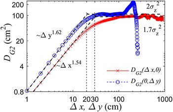
The structure function for the along-conduit (red, x) and cross-conduit (blue, o) direction. X-axis denotes the along-conduit (~9 m) and cross-conduit (~2.8 m) spatial distances, Y-axis is the value of the structure functions.

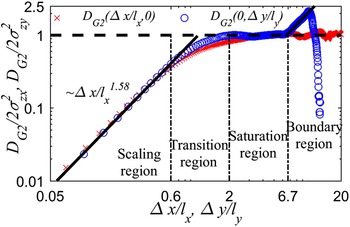
Non-dimensionalized structure function from Figure 6 for along-conduit (red, x) and cross-conduit (blue, o).

2.5. Calculation of slope and aspect from DSMs
Slope and aspect (Fig. 8) are computed from z r at each point in the 1 cm grid using two adjacent along-flow and two adjacent cross-flow points (Hodge and others, Reference Hodge, Brasington and Richards2009).
Polar plot of the slope and aspect at each point in the 9 m conduit segment. Calculations use the four neighboring points of each point. Aspect angle is from 0° to 360° and slope angle is from 0° (center) to 90° (edge). Slopes and aspects are binned into 5° bins and plot is shaded by sample density (dark is high density). Conduit is aligned from 0° aspect (upstream) to 180° aspect (downstream).

2.6. Calculation of relative roughness from DSMs
We compute relative roughness at each cross section (each cm, one shown in Fig. 5) in the 9 m high-resolution segment of the conduit (Fig. 9) from Eqn (2). Roughness r comes from σ z, which is the standard deviation of z r at each cross section, P comes from the path length along the roof and the floor surface z s and A comes from the cross-sectional area calculated by subtracting the z s floor from the roof, and integrating.
Cross-section area A, wetted perimeter P, hydraulic radius D H, standard deviation of roughness heights σ z and relative roughness r r for the 9 m segment shown in Figure 4. The 5% relative roughness threshold is marked as a horizontal gray line in the relative roughness plot.

2.7. Impact of conduit diameter on relative roughness
We use a simple geometric growth model to examine how relative roughness changes in conduits of different diameters. At size s 1cm a conduit with a 1 cm radius is placed at the center of the 3-D model of the conduit floor (z s). At s 2cm, the roof is 2 cm high and twice as wide. Results are not sensitive to the specific shape of the roof, only to its size. This process continues until s 1m, where the roof reaches 1 m high (schematic of three stages of growth is shown in Fig. 5c).
We calculate the relative roughness for each geometry twice, once using a fixed roughness height (the method typically used if a realistic floor surface and roughness model is not available), and once as described in the previous section, but using only the portion of the floor in the conduit (Fig. 5c). We show the mean relative roughness plus and minus one standard deviation as a function of conduit roof height (Fig. 10). The standard deviation comes from the 900 measurements at each geometry step (i.e. 900 cross sections, one at each cm along the 9 m conduit).
Relative roughness verses roof height in cross sections of a ‘growing’ conduit (schematic of growth shown in Fig. 5c). Solid line shows mean (gray band is ±1 standard deviation) relative roughness for roof heights from 0 to 1 m for each cm in Figures 4, 9. Roughness calculated as the standard deviation of the floor elements within the conduit at each geometry step. Dashed line is when roughness heights held constant at 0.07 m.

3. RESULTS
3.1. Conduit description
The 125 m section of subglacial conduit mapped as part of this study begins at the base of the moulin as a large cavern (~6–8 m wide, 2–4 m high, ~30 m long; Table 1). Conduit diameters decreased to 1–2 m a few meters down glacier and conduit widths were slightly less than double the height. The ice roof appeared as a near-perfect Röthlisberger channel (Röthlisberger, Reference Röthlisberger1972) for most of its length, and the floor was almost entirely covered by rocks that ranged in diameter from ~1 cm to 1 m. We did not observe any significant accumulation of particles that were smaller than 1 cm. We observed a few sections of exposed bedrock on the floor.
The downstream portion of the 125 m long conduit segment terminated in a large cavern that was ~15 m wide and ~5 m tall (Table 1). This cavern was the junction of two conduit segments, the other one with a flat ice roof and a near-rectangular shape carved into sediments similar to a Nye channel (Nye, Reference Nye1976). Further downstream, passages became too constricted for human navigation.
Because we do not know when the system was last pipe-full, we do not know the amount of creep closure, although some certainly occurred between the last pipe-full flow and our observations. Our fieldwork did not explicitly measure creep closure, but no closure was noticed during the 10 d span during which we observed the conduit.
3.2. Roughness heights
Near GCP A10, where both hand-count and digital methods were used to define roughness heights, measurements agree within a few cm (a few tens of percent) of each other. Elsewhere, where only the hand-count data were collected, results show no significant change from the A10 region (Tables 2, 3).
3.3. Roughness widths
As discussed in Section 2.4, if the small-scale roughness is isotropic the 2D structure function along any direction, for example. the x- and y-directions in a Cartesian coordinate system, should be identical after non-dimensionalization. Here we report the results of the structure function that tests the hypothesis of isotropic roughness.
Both of the longitudinal (x, along-conduit) and transverse (y, cross-conduit) structure functions follow a power law for small correlation scales, followed by a decrease in the slope before reaching a constant value (Fig. 6). The two power law behaviors are fitted by straight dashed lines with approximately equal powers (difference <4%) and only slightly different constant values. Constant values are  $2\sigma _{zx}^{\rm 2} $ and $2\sigma _{zy}^{\rm 2} $, with σ zx = σ z and σ zy = 0.92σ z with σ z = 7.33 ± 0.47 cm denoting the global standard deviation of the roughness field (see Appendix B).
The nearly equal powers and constants indicate that the roughness field is both approximately isotropic and homogeneous. The intersections of the power law curves and the horizontal constant lines define the correlation scales, denoted by l x and l y, respectively. The oscillation and dip at the end of the transverse (across-conduit) structure function is due to interference when the conduit rock wall in this section, instead of only bed elements, enters the function domain (Fig. 6).
To better understand the characteristics of the structure function, Figure 7 gives the non-dimensionalized (by  $2\sigma _{zx}^2 $ and $2\sigma _{zy}^2 $) structure function with respect to non-dimensionalized (by l x and l y) correlation scales. After non-dimensionalization the two functions overlap except for the boundary region in the transverse direction. We divide the curves into three regions based on their different scaling behaviors. In the scaling region (<0.6), the relationship D G2 (λΔx) = λ 1.58 D G2 (Δx) relates the small-scale to the large-scale features. A transition region from the scaling behavior to the stable value exists between 0.6 and 2. In the final saturation region, the structure function is determined by the DSM boundary. From the above, the non-dimensional curve is uniquely determined by horizontal length scales l x and l y, vertical roughness scales σ zx and σ zy, and a constant power of 1.58 ± 0.04. The constant power is similar to the degree of complexity and irregularity of river beds (Nikora and others, Reference Nikora, Goring and Biggs1998; Aberle and Nikora, Reference Aberle and Nikora2006). The horizontal scales are l x = 29.5 ± 1.5 cm and l y = 20 ± 1 cm (see Appendix B).
3.4. Roughness slope and aspect
Roughness elements (rocks) on the floor appear visually jagged (Figs 2a, 3b) and slopes, mostly <30°, have no apparent preferential alignment (Fig. 8). The region with a high density of large slopes (>60°) facing just downstream of ~ 270° is due to the conduit rock wall near A10 captured near the entrance of this section (Fig. 2).
3.5. Relative roughness
Relative roughness is >5% for >70% of the length of the 9 m conduit segment (boxed region in Fig. 1). Relative roughness variability is primarily controlled by the σ z of the roughness elements, rather than variability in cross-section area and perimeter. A general decrease in cross-section area along the 9 m segment, however, combined with a similar decrease in σ z does move relative roughness from >5% upstream to <5% downstream (Fig. 9).
In this 9 m segment the cross-sectional area changes by a factor of 4 from ~2 to 0.5 m2 over a length equal to a few conduit widths. In other places the channel doubled in height for ~1 m along-conduit and then returned to its previous dimensions.
3.6. Changing relative roughness due to conduit enlargement
When the simple geometric conduit size model is a 1 cm wide and tall conduit, relative roughness has a mean value of ~17% (for 900 cross sections at each cm along the 9 m conduit). However, the range of relative roughness is large (gray band in Fig. 10 denotes 1 standard deviation of the 900 cross sections), including a lower bound of 0 relative roughness for some initial cross sections. Zero percent relative roughness can occur when the conduits are smaller than the size of a roughness element, meaning roughness elements may not be included into the conduit space. Alternatively, the flat surface of a single roughness element may make up the entire conduit floor, and the conduit floor then appears smooth. As the conduit grows and includes roughness elements, the lower bound of relative roughness increases. After the conduit grows to ~20 cm, which is near the roughness element amplitude (Table 2), the standard deviation envelope tightens to within  ${\rm \sim} \pm 5\% $ of the mean. Mean relative roughness is >5% until the conduit roof grows to >1 m high. While the lower bound of the standard deviation envelope is always <5% the upper bound is always >5% for this simplistic growth model in this conduit segment (Fig. 10).
If a constant roughness element size is used regardless of the conduit size (0.07 m, equivalent to the σ z for this region; Table 2), relative roughness is drastically over-estimated during early conduit formation (dashed line in Fig. 10). In fact, when the conduit is <0.07 m high, this simple method estimates >100% relative roughness, or full flow blockage. If the hand-count data were used instead, (0.09–0.22 m, depending on the method used), the results would be similar but the errors even larger.
4. DISCUSSION
Our results show that this subglacial conduit has variable cross-section areas, large roughness elements and high values of relative roughness. This heterogeneity is not captured in existing models that use uniform or spatially smoothed values.
Variability in cross-sectional area determined from cave surveys and photographs suggests variability in heat transfer, melt opening rates, creep closure rates and if mass is conserved, variability in local pressure and velocity. We address the implications of these below. Large changes in cross-sectional area over short distances imply large changes in melt opening via heat production. The processes that led to this inferred localized heat production are not known. We speculate, however, that highly variable cross sections may have formed as a result of turbulent flow structures that are established by very large roughness elements at the glacier bed during pipe-full flow, such as one or more very large rocks. Another possible cause is head losses in currents established by changes in flow direction. In both cases, head losses (and thus heat generation) would be larger in these areas than at other locations downstream. Regardless of the cause, the observation that cross-sectional areas increase and decrease along a conduit contrasts with models that have assumed conduit cross-sectional areas tend toward uniformity.
The presence of constrictions along conduit flow paths would impact patterns of conduit enlargement. From Schoof (Reference Schoof2010),
 $$\displaystyle{{{\rm d}A} \over {{\rm d}t}} \approx c_1 \;Q \Phi - c_2 \;N^n \;A,$$
where dA/dt is the time rate of change of the conduit cross-sectional area A, Q is volumetric flow rate, Φ is hydraulic potential gradient, N is effective pressure and n is a parameter from Glen's law, typically 3 (Cuffey and Paterson, Reference Cuffey and Paterson2010). Constants c 1 (Pa–1) and c 2 (Pa–3 s–1) provide unit equivalency. The two terms on the right-hand side are the melt opening rate and the creep closure rate. Flow constrictions cause higher pressures upstream of the constriction and result in lower pressure downstream, establishing a locally increased pressure gradient across the constricted region. From Eqn (4), sections of a conduit with increased pressure gradient (compared with those with the average gradient) will have increased melt opening. At the same time, the constriction has a decreased area and therefore a decreased creep closure rate. Conversely, the expanded regions of the conduit would open by melting more slowly and close by creep more rapidly. These two complementary processes are generally assumed to create conduits with uniform or slowly varying cross sections. Our observations reveal this is not the case in this conduit, and again suggest that simple treatment of conduits as uniform pipes may not properly capture the likely range and variability of melt opening, creep closure and therefore water pressures in a conduit. The presence of constrictions also highlights the importance of simulating minor head losses, which are typically neglected in models of subglacial conduit hydrology (e.g. Banwell and others, Reference Banwell, MacAyeal and Sergienko2013).
Once established, flow constrictions are likely to migrate. According to Isenko and others (Reference Isenko, Naruse and Mavlyudov2005) and Covington and others (Reference Covington, Luhmann, Gabrovšek, Saar and Wicks2011), heat transfer is not instantaneous in glacier or karst systems. Therefore, excess heat released locally in the water in a constriction would impact the ice farther downstream. Just as the small-scale scallop roughness features on the ice roof migrate downstream (Curl, Reference Curl1974), the large-scale roughness contraction and expansions are likely to migrate too.
Our discovery of flow constrictions implies variability in flow velocity that can impact relative roughness and roughness. Cross-sectional area decreases by a factor of 4 from ~2 to ~0.5 m2, over just a few horizontal meters (Fig. 9). If flux Q is held constant and only a function of velocity, v, and area, A, or Q = v 0 A 0 = v 1 A 1, then a coincident fourfold increase in velocity must occur. This change in velocity may not matter in the context of heat exchange. Covington and others (Reference Covington, Luhmann, Gabrovšek, Saar and Wicks2011) report that increased velocity causes increased turbulent mixing, a smaller convective boundary layer, and increased heat exchange, but this is offset by the shorter residence time due to the increased velocity. Increased velocity, however, increases the ability of the flow to erode, entrain and move sediments and/or roughness elements. Velocity increase through constrictions will remove smaller clasts and increase effective roughness. If large clasts are entrained by flow in constrictions, then they can be moved to locations downstream, where expanded cross-sectional area and decreased flow velocities cause them to accumulate on the floor and increase roughness. Contrary to this, smaller conduits in general have reduced flow compared with larger conduits. However, beyond this speculation, transport is not considered in this work, and our analysis treats the floor as a fixed surface. In reality, both water and ice move roughness elements into and out of the conduit on multiple timescales. It seems reasonable to assume that the smallest grain sizes and sediments not observed were removed by water. The larger elements that were observed may be emplaced and moved by fluvial and/or glacial transport processes.
The roughness widths and comparable d 84 heights reported here are slightly larger than the 15 cm surface roughness height computed from b-axis measurements under a nearby Svalbard glacier reported in Gulley and others (Reference Gulley2014) (our results using the same method are 22 cm (Table 2)). The size of roughness elements was not highly variable along the conduit (Table 3) but large variability in cross-sectional area (Fig. 9 and Table 1), resulted in large changes in relative roughness. An exposed rock wall appears to contribute to the change in area and perimeter in the 9 m high-resolution segment examined in detail here, but elsewhere there is no obvious object that causes the changes in cross-sectional area. Our results suggest therefore that a single roughness element size might be used for parameterization of relative roughness in models of subglacial conduits. Relative roughness values were >5 for >70% of this segment (Fig. 9 bottom), indicating that the radius of a semi-circular conduit would need to exceed 1 m before relative roughness dropped below 5%. One meter is near the size of the conduit we observed, suggesting significant challenges for determining a physical basis for hydraulic roughness evolution in hydrological models of subglacial conduits.
Our results indicate that the distribution of roughness in subglacial conduits is similar to that in rivers. The structure function power law describing roughness has a power of 1.58, which is within the range of 1.5 ~ 1.66 for natural rivers (Nikora and others, Reference Nikora, Goring and Biggs1998). In contrast to most rivers, however, roughness elements do not appear flow-aligned in this conduit. This lack of flow-alignment suggests that the system is fluvially young, which is also supported by the significant angularity of the rocks (Figs 2 and 3). In our case, the angularity of the rocks, lack of imbrication and large variability in clast sizes is most likely a result of clasts derived from winnowing of poorly sorted subglacial diamicts. These clasts accumulate and armor channel floors after removal of finer-grained materials (e.g. Gulley and others, Reference Gulley2014). Other reasons flow-alignment may not occur include high variability in discharge and velocity from a lake drainage event, or conduit closure in winter and ice-induced movement of the rocks. We consider closure unlikely, however, because most of the conduit is under <100 m of ice. Regardless of the cause, angular and non-aligned roughness elements mean that this system is effectively rougher relative to a river that has the same diameter of rocks that are imbricated. The contribution of imbrication to relative roughness is not captured when roughness is calculated by a hand-count method; it is only possible to characterize it using non-disruptive digital scanning methods (Smart and others, Reference Smart, Duncan and Walsh2002).
A simple geometric model used to vary conduit size shows that smaller conduits (representative of earlier in the melt season) are more sensitive to differences in estimates of roughness. The DSM-derived roughness estimates agree with the traditional static roughness estimates. When the conduit is large, relative roughness estimates using either property are similar, and decrease toward 5% as the conduit grows >1 m. However, two differences emerge when conduits are smaller. The first is that a static roughness used in the relative roughness calculation greatly over-estimates relative roughness. When the conduit is less than or equal to the roughness size, this equation predicts 100% relative roughness, implying a blocked conduit. Conversely, the DSM-derived roughness produces relative roughness that remains <35%. The second change is that the range of likely relative roughness increases. In the small conduits examined here, relative roughness may be <35%, but it may be <5%, within 1σ uncertainty. In the larger conduits, uncertainty is only ~5%. This increased uncertainty occurs because there is variability in roughness at each cross section, and results are more sensitive to the roughness property at small scales.
High resolution 3-D representations of subglacial conduits mean that new types of models can be used to examine this system. In addition to applying existing statistical or analytical methods to a new data domain, as was done here, a 3-D representation can be used as the mesh and domain for a computational fluid dynamics (CFD) model. The structure function analysis can help define the mesh resolution and what small-scale objects can be parameterized, versus what objects must be explicitly resolved. One sample application is a simulation to calculate the effective wall roughness term that encapsulates the effects of large relative roughness. This term can then be used in simpler non-CFD models.
Just as our observations have provided evidence of high spatial heterogeneity of conduit cross-sectional area, CFD modeling can move us beyond the assumption of the uniform system commonly modeled. CFD modeling of this system will allow exploration of the effects of small-scale roughness (the individual roughness elements that are discussed throughout this paper) or form roughness (i.e. the 3-D pinch-points, twists and turns in Fig. 1). Distinguishing between these two properties is important because roughness elements are related to the bedrock and likely to be glacier- or region- specific, but form roughness may be related to hydrology and therefore likely to be a more universal feature. Alternatively, at one location roughness elements are approximately steady state on an annual timescale, but form roughness evolves as the conduit melts open.
If we assume the roughness elements observed in the fall were in approximately the same place in the spring, then a CFD model can also improve on our simple geometric model used here and impose a synthetic but reality-based ice roof closer to the floor. It is in this period of early conduit formation, when conduits are small, that additional water is most likely to increase the pressure head, leave the conduit, lubricate the local bed, reduce basal stress, and allow faster ice flow. However, errors in estimated relative roughness are largest when conduits are small. Although existing models using simplified conduits have had great success relating subglacial hydrology to glacier behavior, the transition from non-channelized distributed systems to conduit systems, including the early stages of conduit formation, is not yet fully understood. Roughness elements splitting subglacial flow was suggested as one possible reason for multi-peaked dye-trace curves by Nienow and others (Reference Nienow, Sharp and Willis1998), suggesting that very rough conduits may appear as a distributed system in a dye-trace study. It is likely that proper treatment of the early stages of conduit growth, when relative roughness is large, will require consideration of the spatial heterogeneity of the conduit size, shape and roughness properties presented here.
5. CONCLUSION
We present the first high spatial resolution DSM of a subglacial conduit. The roughness values derived from a digital model are in agreement with traditional hand-count when reduced to a single statistical value. However, a ~9 m long high resolution DSM shows high spatial variability due to the individual rocks on the floor. Analysis of the conduit floor shows no imbrication or flow alignment, yet there appears to be a small difference in along- versus across- flow roughness sizes from a structure function analysis. Relative roughness changes along the conduit were due to both cross-section area changes and to changes in the roughness elements themselves.
In this conduit, relative roughness is >5% in the mature conduit we imaged for >70% of its length, making it difficult to justify use of standard approximations of roughness coefficients from relative roughness, which hold for relative roughness <5%. When the conduit is smaller than what we measured, relative roughness is even larger. The time evolution of the system was not captured in our 3-D representation, which occurred at the end of the melt season. However, we did explore the time evolution using a simple geometric model of conduit sizes. DSM-derived roughness estimate and static roughness estimates produce different results when used in a simple geometric model that explores smaller conduit sizes. When the conduit is smaller than the static roughness size, relative roughness is 100%, which implies flow blockage. When the DSM is used, relative roughness remains well below 100%.
Changes in cross-sectional area along the conduit, including contraction and expansion points and sharp 3-D turns, mean that conduits cannot be easily represented by a straight uniform pipe with uniform wall drag impacting flow. The surface model, deconvoluted roughness field and conduit cross sections presented here show that the standard treatment of roughness parameters is unlikely to be directly related to roughness heights until conduits are large.
ACKNOWLEDGMENTS
K.M., J.G., X.L. and Y.C. were supported by the National Science Foundation (NSF) under Grant No. #1503928. The fieldwork team (K.M., J.G., M.C.) were supported by the Norwegian Arctic Research Council and Svalbard Science Forum, RiS #6106. K.M. was also supported by the National Aeronautics and Space Administration (NASA) Headquarters under the NASA Earth and Space Science Fellowship Program – Grant NNX10AN83H, the University of California, Santa Cruz, and the Woods Hole Oceanographic Institution Ocean and Climate Change Institute post-graduate fellowship. Portions of this work were conducted while J.G. was supported by the NSF EAR Postdoctoral Fellowship (#0946767). S.T. was funded by NASA grant NNX11AH61G. We thank the Polish Research Station and the 2012 winter crew at Hornsund, Svalbard, for their logistical support and hospitality and acknowledge contributions from Mikolaj Karwat and Lucasz Stachnik when hand-counting rocks. Klättermusen provided cold weather gear. We thank Thomsa Whelan for providing a first pass at processing the Kinect data with his Kintinuous algorithm (Whelan and others, 2012), and Raphael Favier for assisting with modifications to KinFu Large Scale. Finally, we thank Anders Damsgaard and the anonymous reviewers who also contributed to the quality of the final manuscript.
APPENDIX A
APPENDIX B
STRUCTURE FUNCTION
To better understand the local roughness scales, the 2-D structure function (Kolmogorov, Reference Kolmogorov1991; Nikora and others, Reference Nikora, Goring and Biggs1998) is introduced to calculate the roughness covariance at two different points. Considering the z s surface and arbitrary boundary, denoted by Γ, of the conduit DSM, and the roughness model z r as a function of space (x,y), the 2-D structure function can be expressed by Eqn (B1) (continuous form),
 $$\eqalign{& D_{{\rm Gp}} (\Delta x,\Delta y) = \langle \vert z_{\rm r} (x + \Delta x,y + \Delta y) \cr & - z_{\rm r} (x,y) \vert ^{\rm p} \rangle, (x + \Delta x,y + \Delta y) \in \Gamma,}$$
and Eqn (B2) (discretized form),
 $$\eqalign{& D_{{\rm Gp}} (\Delta x,\Delta y) = \displaystyle{1 \over N}\sum\limits_i \sum\limits_j \vert z_{\rm r} (x_i + \Delta x,y_j + \Delta y) \cr & \quad - z_{\rm r} (x_i, y_j ) \vert ^{\rm p}, \;(x_i + \Delta x,y_j + \Delta y) \in \Gamma,}$$
where 〈 · 〉 is the mean, p is the order of the structure function, (Δx, Δy) is the correlation location vector and N is the total valid grid points satisfying Eqn (B2).
Equations (B1) and (B2) are equivalent in terms of their physical meaning. The continuous form (Eqn (B1)), is more general but the discrete form (Eqn (B2)) is used here because the roughness field data are discretized.
Generally speaking, the full statistical properties of z r(x, y) can be denoted by the joint probability function (PDF) at all locations. According to previous research in natural rivers (Nikora and others, Reference Nikora, Goring and Biggs1998; Bertin and Freidrich, Reference Bertin and Freidrich2014), the PDFs are close to the Gaussian distribution, and thus, we assume the 2nd-order (p = 2) moment of the roughness height provides the regional scale information.
The global mean and standard deviation of the roughness height r s is  $\overline {z_{\rm r}} = - 1.22 \pm 0.21\;{\rm cm}$ and σ z = 7.33 ± 0.47 cm, respectively. According to the definition of the 2nd-order structure function, $D_{{\rm G2}} (\Delta x \to \infty, \;0) = 2\sigma _{zx}^2 $ and $D_{{\rm G2}} (0,\;\Delta y \to \infty ) = 2\sigma _{zy}^2 $, where σ zx and σ zy are constants. Figure 6 shows the variations of the structure function along x- and y-directions with respect to correlation distances. From Figure 6 the 1-D structure function along x-direction goes to a constant at $1.7\sigma _z^2 $, which means σ zx = 0.9σ z. For the y-direction, the function also tends to a constant (ignoring the boundary-generated noise at the largest scales), and the constant value is $2\sigma _z^2 $, indicating that σ zy = σ z. For the special case of a homogeneous roughness field, σ zx = σ zy = σ z. The current roughness field is therefore not entirely homogeneous. However, considering the possible errors from 3-D DSM construction from 2-D photos, large-scale detrending and sampling and resampling during numerical calculations, we claim the roughness field is approximately homogeneous before it reaches the boundary regions.
APPENDIX C
UNCERTAINTY AND ERRORS
Grid resolution
Results are not sensitive to the grid resolution as seen from the high point density in the gridded product. The average grid cell has a point density of 12 points cm–2 and a standard deviation of 2 cm. The plan-view grid does skew these statistics slightly, because vertical surfaces are ‘collapsed’ and give high point density and high standard deviation (Fig. 11).
Point density (a, b) and standard deviation of values (b, c) of SfM data after on a the 1 cm resolution grid. Panels (a) and (c) show plan view with spatial distribution of density and standard deviation, respectively. Panels (b) and (d) show a histogram of the distribution of the points from (a) and (c), respectively.

Window size
The 30 cm Gaussian window used to deconvolute the DSM into the z s floor and the z r roughness surface has an effect on the z r surface and therefore the analysis. Here we demonstrate that the effect is small by repeating parts of the analysis with the window size changed by  $ \pm 10\% $, from 27 to 33 cm.
1. Impact of window size on the structure function
The correlation scale for the structure function is weakly dependent on the moving window used to deconvolute the floor. The dividing scale defines the value at which the power curves meet the constants of the curves at higher scales.
From Table 4, we compute the uncertainty due to the deconvolution window size w as:
• power (x): 1.52 ± 0.03. Uncertainty <2%.
• power (y): 1.61 ± 0.04. Uncertainty <2.5%
• l x: 30 ± 6 cm. Uncertainty <20% for w ± 10 cm
• l x: 29.5 ± 1.5 cm. Uncertainty <5% for w ± 10%
• l y: 20 ± 3 cm. Uncertainty <15% for w ± 10 cm
• l y: 20 ± 1 cm. Uncertainty <5% for w ± 10%.
Effect of variable Gaussian window size for surface deconvolution. Baseline size is 30 cm, and we examine the impact of  $ \pm 10\% $ and ±10 cm on the power law exponent, l x, l y and structure-function derived σ z and $\overline {z_{\rm r}} $ results

Based on these results, we claim the power laws are not sensitive to the window size as the relative error is within 2.5% for both powers. To accurately determine the horizontal scales, a proper window size should be chosen, which means selecting what portion of the DSM is the ‘surface’ and what portion is the ‘roughness’, which does not have a well-defined solution, especially for complex curved 3-D surfaces. In this paper, the window size of 30 cm is appropriate as the relative errors for all parameters of interest are within 5%, although anything from 25 to 35 would produce similar results.
2. Impact of window size on deconvolution of z s floor and z r roughness
Changing the window size by 10% produces a mean change in the z r roughness surface of 2 mm. A graphical view of the changing deconvolution window is shown in Figure 12. In some places, especially near the vertical wall, the new surface is different by >1 cm. However, this does not represent a ‘new’ 1 cm roughness feature, as the change varies slowly in the spatial dimension due to the window size. This is instead an accumulating trend in the z r surface. Further analysis using this surface, for example the geometric growth model, is not significantly impacted by these 10% changes in window size.
Plan view of conduit floor surface z s and roughness element z r differences based on different smooth window size. (a) and (b) are the change in the z s surface with a ±10% change from the 30 cm moving window size (27 and 33 cm, respectively). (c) and (d) are the residual z r surface differences. Axis units are m as in Figure 4, contour lines and labels are every cm.


 Open access