


Introduction
The potential of the Antarctic Ice Sheet (AIS) to raise global sea levels by up to 58 m (Fretwell and others, Reference Fretwell2013) means that understanding the impacts of a warming climate on the southern polar region is one of the grand scientific challenges of our time (Bell, Reference Bell2008). The extent of the AIS is sensitive to change in both the atmosphere and the ocean (Whitehouse and others, Reference Whitehouse, Gomez, King and Wiens2019). The vulnerability of the AIS underscores the need for more accurate ice-sheet models, these are crucial for understanding ice dynamics and future ice flow variations. Geothermal heat flux (GHF) is an important thermal boundary condition in these models because it affects the temperature at the base of the ice sheet and is the dominant control on basal temperatures in slow-flowing areas (Larour and others, Reference Larour, Morlighem, Seroussi, Schiermeier and Rignot2012; Pittard and others, Reference Pittard, Roberts, Galton-Fenzi and Watson2016). Ice flow is sensitive to the local spatial variation of underlying GHF, especially near ice divides and at the edge of ice streams (Bell and others, Reference Bell, Studinger, Shuman, Fahnestock and Joughin2007; Pittard and others, Reference Pittard, Roberts, Galton-Fenzi and Watson2016). In turn, the heat supplied to the base of the ice sheet influences the rate of internal ice deformation (Budd and Jacka, Reference Budd and Jacka1989; Durand and others, Reference Durand2007). The GHF also modulates the production of basal meltwater that can lubricate the bedrock–ice interface and lead to faster ice velocities and increase discharge (Näslund and others, Reference Näslund, Jansson, Fastook, Johnson and Andersson2005; Pattyn, Reference Pattyn2010). Local GHF is also a first-order consideration in site selection for climate records, especially in the search for ‘old’ (million-year) ice core sites. Locations where ice is at pressure melting point can lead to melt-driven erosion of the glacial stratigraphy, reducing the temporal range of the climate record (Fischer and others, Reference Fischer2013; Liefferinge and Pattyn, Reference Liefferinge and Pattyn2013; Parrenin and others, Reference Parrenin2017; Karlsson and others, Reference Karlsson2018).
GHF is the sum of heat generated by mantle convection and conducted through the lithosphere and the heat generated by radiogenic decay of heat-producing elements within the lithosphere. These elements are mainly uranium, thorium and potassium which together produce 98% of the lithospheric heat from radiogenic decay (Pollack, Reference Pollack1982). With direct access to the bedrock, GHF (q(0)) is estimated by multiplying the vertical temperature gradient of the subsurface (∂T/∂z) and the thermal conductivity of the rock (K) (Turcotte and Schubert, Reference Turcotte and Schubert2014):

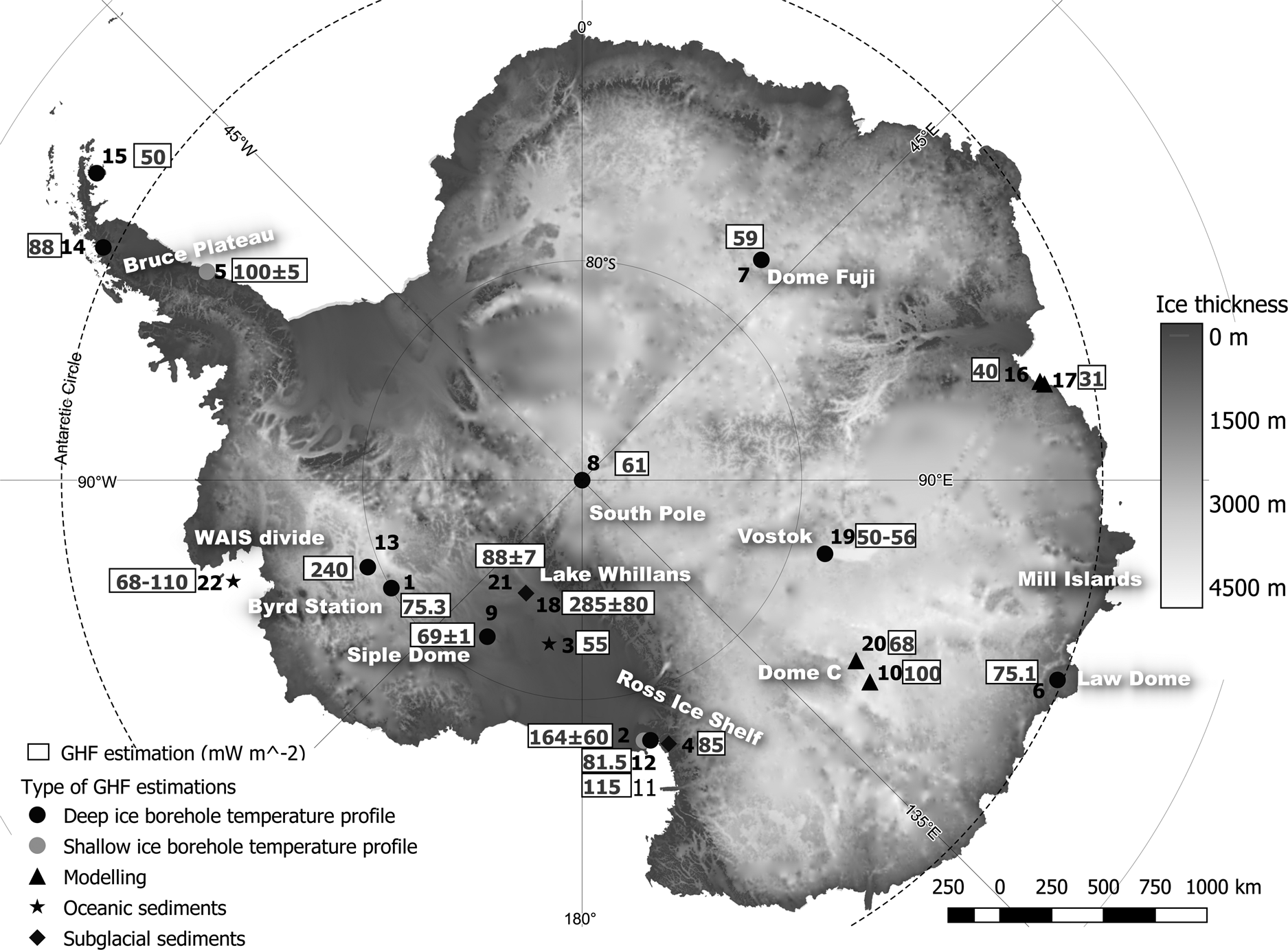
In Antarctica, GHF is one of the most difficult parameters to constrain because accessing subglacial bedrock and continental shelves is logistically challenging due to kilometres-thick ice cover. Few in-situ GHF measurements have been attempted, and all of them are located under the West Antarctic Ice Sheet (WAIS) in subglacial sediments (e.g. Morin and others, Reference Morin2010; Fisher and others, Reference Fisher, Mankoff, Tulaczyk, Tyler and Foley2015; Begeman and others, Reference Begeman, Tulaczyk and Fisher2017) or oceanic sediments (e.g. Dziabek and others, Reference Dziadek, Gohl, Diehl and Kaul2017) (Fig. 1). For East Antarctica, there are GHF estimates derived from ice-borehole temperature profiles (Fig. 1), but no measurements have yet been reported from bedrock or subglacial sediments.
Location of deep temperature profile boreholes and different local GHF estimations. Ice-sheet thickness data from BEPMAP 2 (Fretwell and others, Reference Fretwell2013) and Basemap from Quantarctica and the Norwegian Polar Institute 1: Gow and others (Reference Gow, Ueda and Garfield1968); 2: Risk and Hochstein (Reference Risk and Hochstein1974); 3: Foster (Reference Foster1978); 4: Decker and Bucher (Reference Decker and Bucher1982); 5: Nicholls and Paren (Reference Nicholls and Paren1993); 6: Dahl-Jensen and others (Reference Dahl-Jensen, Morgan and Elcheikh1999); 7: Hondoh and others (Reference Hondoh, Shoji, Watanabe, Salamatin and Lipenkov2002); 8: Price and others (Reference Price2002); 9: Engelhardt (Reference Engelhardt2004); 10: Carter and others (Reference Carter, Blankenship, Young and Holt2009); 11: Morin and others (Reference Morin2010); 12: Schröder and others (Reference Schröder, Paulsen and Wonik2011); 13: Clow and others (Reference Clow, Cuffey and Waddington2012); 14: Zagorodnov and others (Reference Zagorodnov2012); 15: Mulvaney and others (Reference Mulvaney2012); 16 and 17: Carson and others (Reference Carson, McLaren, Roberts, Boger and Blankenship2014); 18: Fisher and others (Reference Fisher, Mankoff, Tulaczyk, Tyler and Foley2015); 19: Dmitriev and others (Reference Dmitriev, Bolshunov and Podoliak2016); 20: Parrenin and others (Reference Parrenin2017); 21: Begeman and others (Reference Begeman, Tulaczyk and Fisher2017); 22: Dziabek and others (Reference Dziadek, Gohl, Diehl and Kaul2017) (26 measurements).
Several studies have attempted to map Antarctic GHF using different methods, including: (1) interpolated geophysical models using either seismic velocities (e.g. Shapiro and Ritzwoller, Reference Shapiro and Ritzwoller2004; An and others, Reference An2015) or magnetic data (e.g. Maule and others, Reference Maule, Purucker, Olsen and Mosegaard2005; Purucker, Reference Purucker2013; Martos and others, Reference Martos2017), (2) geological and structural properties of the bedrock (e.g. Carson and others, Reference Carson, McLaren, Roberts, Boger and Blankenship2014; Burton-Johnson and others, Reference Burton-Johnson, Halpin, Whittaker, Graham and Watson2017), (3) the properties within and at the base of the ice sheet (e.g. Siegert and Dowdeswell, Reference Siegert and Dowdeswell1996; Shroeder and others, Reference Schroeder, Blankenship, Young and Quartini2014) and (4) a combination of available models (e.g. Liefferinge and Pattyn, Reference Liefferinge and Pattyn2013). The maps produced by these models allow us to understand the regional variation in GHF, especially the differences between East and West Antarctica, but they are unable to predict local variations due to a limited resolution typically tens to hundreds of kilometres. Indeed, the actual spatial variation of GHF can be on a scale of few kilometres due to local geological contrasts, hydrothermal circulation and volcanic activity (Carson and others, Reference Carson, McLaren, Roberts, Boger and Blankenship2014; Begeman and others, Reference Begeman, Tulaczyk and Fisher2017). Furthermore, continent-wide geophysical models use simplified lithospheric parameters including laterally homogeneous radiogenic heat production, although this is known to vary with rock type (e.g. Hasterok and others, Reference Hasterok, Gard and Webb2017) and has been estimated to contribute up to 70% of total surface GHF on the Antarctic Peninsula (Burton-Johnson and others, Reference Burton-Johnson, Halpin, Whittaker, Graham and Watson2017). The fact that GHF is currently not well-constrained is evident in the inconsistencies between different GHF models.
GHF estimates from the ice sheet
The temperature of the ice sheet at different depths is a good indicator of past surface temperature variation because, over the years, the heat from the surface is conducted and advected into the ice sheet and this leaves an imprint on the ice temperature (e.g. Dahl-Jensen and others, Reference Dahl-Jensen1998). GHF will also affect the temperature of the ice sheet by providing a source of heat at the bottom of the ice. By measuring the temperature profile of the ice sheet and compensating for heat from the bedrock, it is possible to reconstruct a smoothed version of surface temperature history and estimate GHF. However, using ice-borehole temperature profiles to estimate GHF is challenging because the heat generated at the bottom of the ice sheet can be produced from several sources, especially when the ice sheet is moving horizontally. Ice flow can produce shear heating, heat advection and basal frictional heating which could affect the temperature of the ice sheet (Engelhardt, Reference Engelhardt2004; Pittard and others, Reference Pittard, Roberts, Galton-Fenzi and Watson2016). Bedrock topography also has an impact on GHF magnitude at a specific location by concentrating the heat in an area where there is small-scale sharp variation in the slope of the bedrock, like a narrow deep valley, which focusses and increases the basal temperature (Van der Veen and others, Reference Van der Veen, Leftwich, Von Frese, Csatho and Li2007). In an environment with basal melting, this estimation would be a minimum value because the heat used to melt the ice is lost in our model (see section Assumption). These factors should be considered when GHF is modelled from borehole temperature data.
Deep ice-borehole temperature profiles have been measured across Antarctica (Fig. 1) and GHF has been derived from some of these profiles (e.g. Dahl-Jensen and others, Reference Dahl-Jensen, Morgan and Elcheikh1999; Hondoh and others, Reference Hondoh, Shoji, Watanabe, Salamatin and Lipenkov2002; Engelhardt, Reference Engelhardt2004; Clow and others, Reference Clow, Cuffey and Waddington2012). The differences between these ice-borehole estimations of GHF and available geophysically-derived GHF models are significant. For example, Clow and others (Reference Clow, Cuffey and Waddington2012) calculated a value of 240 mW m−2 (Fig. 1) in the central portion of the WAIS, this is higher than the values modelled by any geophysically-derived models. Martos and others (Reference Martos2017) estimated the highest value for this area at approximately 120 mW m−2. However, Clow and others (Reference Clow, Cuffey and Waddington2012) did not account for horizontal flow effects related to bedrock topography and the GHF estimation could have been lower than the one they produced. Figure 2 shows the differences between estimated GHF from various studies at locations where deep ice-borehole temperature profiles are available (Fig. 1). GHF estimations for the East Antarctic Ice Sheet (EAIS) display a relatively narrow range, standard deviations are between 5.9 mW m−2 for South Pole/Vostok and 7.9 mW m−2 for Law Dome/Dome Fuji. The WAIS displays a larger range of GHD estimates, especially the WAIS divide and Byrd Station, where the standard deviation are 24.5 and 25.1 mW m−2, respectively.
GHF values from available continent-wide GHF maps for deep ice borehole locations in Antarctica (see Fig. 1).

This study provides an understanding of the variation of the GHF estimation as a function of the depth of ice-borehole temperature profile. Here we analyse a 1177 m ice-borehole temperature profile from Law Dome and derive a revised GHF estimate using a heat diffusion-advection equation in the ice sheet integrated into a numerical model which includes a forward and an inverse model. The use of a two-step numerical model to estimate surface temperature history from an ice-borehole temperature profile has been performed previously (e.g. Cuffey and others, Reference Cuffey1995; Dahl-Jensen and others, Reference Dahl-Jensen, Morgan and Elcheikh1999; Muto and others, Reference Muto, Scambos, Steffen, Slater and Clow2011; Orsi and others, Reference Orsi, Cornuelle and Severinghaus2012; Roberts and others, Reference Roberts2013). We then systematically truncate the temperature profile from the base upwards, sequentially calculating a new GHF and its associated uncertainties, until the shallowest hundred metres. We explore how the accuracy of modelled GHF changes with depth, including the minimum depth required to discriminate among available geophysical GHF models at the Law Dome borehole location (Dome Summit South; DSS) (Fig. 2). We then explore the regional applicability of this analysis with comparisons to the Dome Fuji and WAIS divide ice core sites (WDC) (Fig. 1). Finally, the impact of the different assumptions used in the model on the final GHF estimation is assessed.
Measurements
Law Dome
To mitigate the impact of horizontal flow, the Dome Summit South (DSS) profile has been measured 4.6 km from the summit of the Dome (Fig. 1), where the horizontal velocity of the ice sheet is assumed to be minimal and the environment approximates a steady state (Morgan and others, Reference Morgan1997; Dahl-Jensen and others, Reference Dahl-Jensen, Morgan and Elcheikh1999). Furthermore, the DSS borehole has been drilled in an area of relatively level bedrock which limits the impact of topography on GHF measurement (Morgan and others, Reference Morgan1997). In 1996, when the DSS temperature profile was measured, the mean annual air temperature was -21.8oC, this precludes melting of the snow at the surface during summer. The recent average accumulation rate was 0.679 m ice a−1 (Morgan and others, Reference Morgan1997). The thickness of the ice sheet is 1220 ± 25 m (Morgan and others, Reference Morgan1997) and the temperature profile stopped around 20 m above the bedrock (Fig. 3). The ice equivalent thickness of the profile is 1176.8 m (Morgan and others, Reference Morgan1997; Dahl-Jensen and others, Reference Dahl-Jensen, Morgan and Elcheikh1999).
Ice-borehole temperature profiles for Law Dome (DSS site) (Morgan and others, Reference Morgan1997), Dome Fuji (Hondoh and others, Reference Hondoh, Shoji, Watanabe, Salamatin and Lipenkov2002) and West Antarctic Ice Sheet Divide (Clow and others, Reference Clow, Cuffey and Waddington2012).

Dome Fuji
At Dome Fuji, a temperature profile has also been measured on a topographic high and this profile reached the bedrock at an ice thickness of 3090 m. Since 2002, the average accumulation rate is 0.032 m ice a−1 (Hondoh and others, Reference Hondoh, Shoji, Watanabe, Salamatin and Lipenkov2002).
West Antarctic Ice Sheet divide
The WDC temperature profile is located 24 km away from an ice divide where it is also considered to have minimal horizontal velocity. A horizontal velocity of 3 m a−1 has been measured by Koutnik and others (Reference Koutnik2016) and the impact of this on the GHF estimation is discussed in the Assumptions section. The deepest temperature recorded was at 3327 m and ice was recovered up to 3405 m (Buizert and others, Reference Buizert2015). The accumulation rate is 0.3 m ice a−1 (Koutnik and others, Reference Koutnik2016).
Steady-state environment
The assumption of a steady-state flow environment has been tested after the modelling at the three locations by comparing the observed surface to basal temperature difference with a steady-state theoretical thermal estimate (Cuffey and Paterson, Reference Cuffey and Paterson2010),

where ΔT is the temperature difference between the top and the bottom of the temperature profile, h is the vertical distance in metres and K is the thermal conductivity of the ice. θB is a dimensionless parameter for temperature which gives the temperature difference between the surface and the base of the ice sheet using the following equation:

where γ is the advection parameter (Cuffey and Paterson, Reference Cuffey and Paterson2010). K and θB have been calculated using the average temperature (T) measured by the different temperature profiles. The temperatures measured at the base and the surface are also derived from the same profiles. The GHF used in this equation is the one that has been estimated by our model.
At Law Dome, for a perfect steady-state environment, the temperature difference between the beginning and the end of the profile must be 10.42 °C, which is lower than the measured temperature difference of 14.3 °C. It shows that the environment is not in a perfect steady state, but the two values are similar and we use this to justify an assumption of a steady-state flow environment within our model. For Dome Fuji the calculated temperature difference is 49.16 °C which is close to the measured difference of 55.3 °C. For the WDC site, the calculated temperature difference is 32.62 °C and the measured difference is 21.29 °C, clearly the assumption of steady state is less valid at the WDC site. Even if this assumption is not entirely valid, we use it to simplify our model. We assess the impact of this assumption on the model results in the section Assumptions.
Method
Heat flow model
To estimate GHF values, a numerical model has been developed which combines: (1) a forward numerical model that reconstructs an ice temperature profile from a given surface temperature history, GHF, accumulation rate and (2) an inverse model which updates the surface temperature history and GHF to minimise the error between the measured and estimated temperature profile. To analyse how shallow a temperature profile can be while still allowing a sufficiently accurate estimation of the GHF value, we use a temperature profile systematically truncated at increasingly shallower intervals. The top 100 m of the observed temperature profile is not included because it is dominated by recent changes in climate and accounting for this introduces too many additional free parameters in the inverse model with associated significant increases in computational cost.
To solve how heat flows through and in the ice, a series of prescribed surface temperature combinations and GHF values are used as boundary conditions in a heat flow model. A one-dimensional finite difference approximation to the heat diffusion-advection equation is used to estimate the temperature profile in the ice. To minimise the difference between the simulated temperature profile and observed one, the inverse model uses particle swarm optimisation with polishing (see section Inverse model) to minimise the value of the regularised root mean squared error (E rms):

where λ is the regularisation parameter, T m is the temperature simulated by the model and T o the temperature measured in the borehole in kelvin, n is the number of data points and ∂2T/∂t 2 is the second derivative of surface temperature with respect to time. The first term is the usual RMS error and the second term is the regularisation term which enforces a degree of smoothness in the model surface temperature function by reducing the impact of overfitting values. Overfitting values could cause problems because they tend to capture local signal variations and noise in the dataset obscuring a general trend.
The change of temperature over time in the ice sheet is controlled by diffusion, advection, firn densification and a correction to the diffusive term due to variations in the thermal conductivity (Cuffey and Paterson, Reference Cuffey and Paterson2010). The heat flow equation used to simulate the variation in temperature of the ice through time,

does not include horizontal advection because sites chosen have minimal horizontal velocity (Johnsen and others, Reference Johnsen, Dahl-Jensen, Dansgaard and Gundestrup1995; Dahl-Jensen and others, Reference Dahl-Jensen, Morgan and Elcheikh1999).
The specific heat capacity (C) of the ice in J kg−1 K−1,

is dependent on the temperature (T) in kelvin. The firn densification energy term (f) (J m−3 s−1) is given by:

The thermal conductivity, in W m−1 K−1, is also dependent on the temperature. It follows Eqns (8) and (9) for the firn (Cuffey and Paterson, Reference Cuffey and Paterson2010), where K i is the thermal conductivity of the pure ice and ρ is the density in kg m−3,


and Eqn 10 for the ice (Cuffey and Paterson, Reference Cuffey and Paterson2010):

The vertical flow of the ice for DSS site equation (w z,t) is from Dansgaard and Johnsen (Reference Dansgaard and Johnsen1969) and is based on a vertical strain rate which is constant in the upper part of the ice sheet, then decreases linearly towards the bedrock (Morgan and others, Reference Morgan1997; Dahl-Jensen and others, Reference Dahl-Jensen, Morgan and Elcheikh1999):

where H is the thickness of the ice sheet and is assumed to be constant in time. The resulting vertical velocity profile is only dependent on the accumulation rate (a(t)). The accumulation rate for the DSS site, which varies in time depending on the surface temperature (T sur(t)), is based on Dahl-Jensen and others (Reference Dahl-Jensen, Morgan and Elcheikh1999) model:

where the recent average accumulation rate (a 0) and the temperature at the surface (T 0) at the time the temperature profile was measured are 0.69 m ice a−1 and − 21.8 °C, respectively. α is the change of accumulation per °C. According to Dahl-Jensen and others (Reference Dahl-Jensen, Morgan and Elcheikh1999) this value is around 7% for the DSS site, which falls in between the α range in general global circulation models (3–4%) and the one for polar models (10%). We used the same α for Dome Fuji and WDC, because we considered both sites to be in a similar environment.
Initial and boundary conditions
The thermal boundary conditions of the forward model are the GHF and prescribed surface temperature history for a period of 50 ky at the surface of the ice sheet. We use a piecewise linear surface temperature history function composed of five temperature values to produce a general trend of the surface temperature history and to mitigate the impact of non-unique solutions due to the presence of high-frequency variation of surface temperature through time. During a certain time period, the surface temperature diffuses in the ice sheet and affects the temperature profile. At deeper locations, the effect of surface temperatures on englacial temperatures is less intense and the initial high-frequency variations spread out and can be produced by a wide range of values (Dahl-Jensen and others, Reference Dahl-Jensen, Morgan and Elcheikh1999; Roberts and others, Reference Roberts2013).
The bedrock is considered as a granite and its properties are listed in Table 2. The type of rock used in the model and its impact on the final estimation of GHF at Law Dome are assessed in the discussion in section Assumptions. The GHF is a boundary condition at the bottom of a layer of bedrock 1300 m thick where it is assumed to be the only source of heat and the surface temperature variation does not have an impact. To calculate the temperature profile in the 1300 m thick layer of bedrock (Table 2), Eqn (1) is used. GHF of the rock underneath the ice sheet (q(0)) is going to be updated by the inverse model to produce the best temperature profile.
Parameters used for testing the steady-state assumption


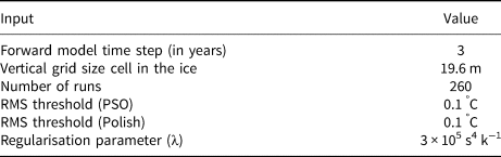
To produce a robust result without being computationally expensive, the model is run several times to optimise the time step, the grid cell size in the ice, the regularisation term (λ) and the number of repetitions during each simulation (Table 3). We picked the value that gave robust results with an acceptable Erms. For λ, the best value is obtained when there is a balance between the regularised and the standard error.
Optimised input values in the ice
Inverse model
In the inverse model, the optimisation is divided into two main steps which are particle swarm optimisations and subsequent steepest descent polish. Particle swarm optimisation improves a set of solution according to a list of criteria by moving particles towards the best solution possible by iteration. It is used to update prescribed temperature history and the GHF value, and to minimise the E rms (Eqn (4)). Particle swarm optimisation allows a good investigation of the search space with a focus on areas that produce the best result possible. For this study, we use 8 swarm members and 250 iterations where each member is assigned a velocity vector which has a random and a momentum component. After evaluating all the criteria for the actual data set, the velocity is adjusted for the next iteration according to how far the particle is from the best solution. The temperature history and GHF that produce the lowest E rms is kept if the E rms is below the error threshold of 0.1 °C, if not the whole iteration process restarts with the same initial boundary conditions. To further minimise E rms we polish the results using direct descent optimisation from the particle swarm optimisation solution results. The steepest descent polish finds the nearest local minimum of a function by computing a new gradient at every iteration to help the model converge. This optimisation is done 100 times, or until the difference between the previous and actual E rms is sufficiently small.
Discussion
For each ice core site, we truncated ice-borehole temperature profiles at different depths. This allowed us to produce several probability distributions of GHF values using a one-dimensional finite difference approximation of the heat diffusion-advection equation. We explore the impact of the depth of a measured ice-sheet temperature profile on the median GHF estimation at specific locations.
Dome Summit South, Law Dome
At DSS, using the whole temperature profile (LD100), the median GHF estimation is 72.0 mW m−2 with a median absolute deviation (MAD) of ± 3.2 mW m−2 (Fig. 4). MAD is a robust estimation of the variability of a probability distribution because it is less impacted by outliers than the standard deviation (SD), which is 1.4826 × MAD if the population follows a normal distribution. We also calculate the percentage of difference between values by using the following equation:

The LD100 value is 4.21% lower than the one estimated by Dahl-Jensen and others (Reference Dahl-Jensen, Morgan and Elcheikh1999) of 75.1 mW m−2, but the difference between the two estimations is within ±1 MAD of LD100 GHF estimation. The differences between the two models are the optimisation technique and the surface boundary conditions. The surface temperature history used in our model follows a piecewise linear function with five points which, combined with the regularisation term added in the E rms equation, decreases the impact of sharp, but short, variation of temperature by smoothing the surface temperature history.
GHF estimation for DSS site from 260 iterations of our model by using a temperature profile of 1176.8 m ice equivalent depth.

To explore the effect of temperature profile depth on acceptable GHF median values we compare the different probability distributions from truncated temperature profiles with the LD100. With a temperature profile depth as shallow as 57% of the thickness of the ice sheet (LD57), the median GHF is 75.5 mW m−2 (Fig. 5). We consider this value to be the shallowest acceptable because it is at the limit of ±1 MAD of the LD100 estimation and more than 60% of the two density distributions overlap. A temperature profile which is half the thickness of the ice sheet gives an estimation of GHF that is 8.13% of LD100 estimation and is within ±2 MAD. The difference increases with shallower temperature profiles, reaching ±9.5 MAD for a temperature profile of 20% total ice thickness (LD20). With LD20, the difference with the GHF median value using the full temperature profile (LD100) is around 35.5% and only 7% of the two probability distributions overlap, indicating that few GHF values from the LD20 models are considered acceptable (Fig. 6).
(A) GHF median values with their MAD for the DSS site using temperature profile truncated at different depths. (B) GHF estimation from Dahl-Jensen and others (Reference Dahl-Jensen, Morgan and Elcheikh1999), Martos and others (Reference Martos2017), Liefferinge and Pattyn (Reference Liefferinge and Pattyn2013), Shapiro and Ritzwoller (Reference Shapiro and Ritzwoller2004).

Comparison between the probability distribution at DSS for the entire temperature profile (LD100) and 20% of the temperature profile (LD20).

Regional applicability
To analyse the regional applicability of the DSS model, we use a modified model at Dome Fuji and WDC to estimate GHF. The ice-borehole temperature profile of Dome Fuji and WDC is located at the summit of a dome and near an ice divide, respectively, where the horizontal velocity is considered to be zero (Fig. 1). The main difference between the DSS model and the one used for the two other locations is the vertical velocity equation:

Also, the E rms thresholds for both locations are higher than DSS. The Dome Fuji threshold is 0.35 °C because the uncertainty of the measured ice-borehole temperature data is approximately 20 times higher for Dome Fuji than for the DSS site. For WDC, it is between 0.9 and 0.2oC, depending on the length of the profile. The WDC site is far enough from the ice divide that some of the assumptions used in the model are not entirely valid, especially the assumption of a steady-state environment.
For DSS, as the temperature profile is truncated, the median GHF shifts to a higher value and the MAD increases; this makes the value less reliable (Fig. 5). At Dome Fuji, GHF estimations decrease with increasing MAD values for shallower temperature profiles (Fig. 7). At WDC, GHF median estimations shift to lower values until approximately half of the temperature profile is used, and then shift to higher GHF values with an MAD following the same behaviour (Fig. 8). The median GHF estimated by our model using the whole temperature profile at Dome Fuji (DF100) is 50.4 mW m−2 with an MAD of 0.9 mW m−2, this is ≈16% lower than that estimated by Hondoh and others (Reference Hondoh, Shoji, Watanabe, Salamatin and Lipenkov2002) of 59 mW m−2. The difference between the two values could be explained by the difference in the method used in our model and that of Hondoh and others (Reference Hondoh, Shoji, Watanabe, Salamatin and Lipenkov2002). In fact, Hondoh and others (Reference Hondoh, Shoji, Watanabe, Salamatin and Lipenkov2002) used a local δ18O record to estimate a GHF value, instead of using the ice-borehole temperature profile. For Dome Fuji, the temperature profile must be at least 90% of the thickness of the ice sheet (DF90) to give an acceptable GHF median value (within ±1 MAD of the DF100 value). For WDC, the median GHF for the whole profile (WDC100) is 90.5 mW m−2 with an MAD of 1.2 mW m−2 and 91% of the whole temperature profile is required in order to be within ±1 MAD of WDC100 value. However, the MAD for DF100 and WDC100 is smaller than LD100. Using the LD100 MAD of 3.2 mW m−2, Dome Fuji requires a temperature profile of at least 80% of the total ice thickness and more than 91% for WDC.
(A) GHF median values with their MAD for Dome Fuji by using temperature profile truncated at different depths. (B) GHF estimation from Martos2017: Martos and others (Reference Martos2017), Liefferinge2013: Liefferinge and Pattyn (Reference Liefferinge and Pattyn2013), Shapiro2004: Shapiro and Ritzwoller (Reference Shapiro and Ritzwoller2004), Hondoh2002: Hondoh and others (Reference Hondoh, Shoji, Watanabe, Salamatin and Lipenkov2002).

(A) GHF median values with their MAD for WAIS divide by using temperature profile truncated at different depths. (B) GHF estimation from Martos2017: Martos and others (Reference Martos2017), Liefferinge2013: Liefferinge and Pattyn (Reference Liefferinge and Pattyn2013), Shapiro2004: Shapiro and Ritzwoller (Reference Shapiro and Ritzwoller2004).

The median GHF behaviour is different at the three locations. The change in surface temperature and accumulation through time has an impact on the ice-sheet temperature profile which might not have reached equilibrium yet (Engelhardt, Reference Engelhardt2004). For example, in an environment with no horizontal velocity, a constant thickness and an accumulation rate of 0.07 m a −1, Cuffey and Paterson (Reference Cuffey and Paterson2010) show than 10 ka after an abrupt but persistent increases of the surface temperature of 15 °C, the ice sheet still contains a signature of the temperature variation at 1000 m below the surface. However, an increase of the accumulation rate to 0.3 m a −1 increases the speed of the propagation of the surface temperature in the ice sheet and the imprint is visible ≈2000 m below surface (Cuffey and Paterson, Reference Cuffey and Paterson2010). At Law Dome, the ice sheet is ≈1200 m thick and the accumulation rate is higher than 0.3 m a −1 (Morgan and others, Reference Morgan1997). The DSS results are considered to be robust because, according to Dahl-Jensen and others (Reference Dahl-Jensen, Morgan and Elcheikh1999), there is no remnant of cold from the past glacial cycle at the bottom of the ice sheet. In several studies δ18O in the ice is used as a proxy for past surface temperature (e.g. Hondoh and others, Reference Hondoh, Shoji, Watanabe, Salamatin and Lipenkov2002). This is achieved by measuring the isotopic ratio oxygen/hydrogen in the ice core and comparing it with a standard value (e.g. Alley and Bentley, Reference Alley and Bentley1988; Dahl-Jensen and others, Reference Dahl-Jensen, Morgan and Elcheikh1999; Watanabe and others, Reference Watanabe2003). Using an ice-borehole temperature profile, instead of δ18O, to analyse past temperature history, limits error to the differing attenuation/suppression of high-frequency information between observations and modelling associated with the calibration of the observed data and past temperature. In contrast, the ice sheets at Dome Fuji and WDC are greater than 3000 m thick (>2.5 times thickness of Law Dome) and likely contain the imprint of multiple glacial cycles that still affects the temperature of the ice at depth. The cold temperatures of the last glacial cycle might still have an impact on the temperature profile at these two locations which would serve to lower temperature values below those assumed in a steady-state environment. In low accumulation rate environments like Dome Fuji (Hondoh and others, Reference Hondoh, Shoji, Watanabe, Salamatin and Lipenkov2002), the vertical strain rate is minimal, and this lowers the advection velocity in the ice sheet. In contrast, the WDC temperature advection velocity is faster, due to a higher accumulation rate (Koutnik and others, Reference Koutnik2016). Consequently, the impact of past glacial cycles decreases more rapidly. At Dome Fuji and WDC, the ice-sheet temperature profiles are more affected by downwelling surface perturbation than at Law Dome, which in turn affects the steady-state thermal regime of the ice sheet at these locations. In the absence of glacial cycles, the reduced advection of cold from the surface at Dome Fuji compared to Law Dome and WDC would result in the GHF dominating the vertical temperature distribution at relatively shallower depths. However, the large glacial cycle variations in surface temperature leave an imprint at Dome Fuji, complicating this interpretation. These factors account for the differences between the three locations and explain why Dome Fuji and WDC require a deeper temperature profile to produce an acceptable GHF value. The estimation of GHF from truncated temperature profiles should therefore be undertaken with caution. Each profile, depending on the maximum depth reached, does not contain the same information. Especially, the surface temperature history and the initial conditions due to the impact of past glacial cycles and intense variation of temperature that could have affected the temperature profile in the ice (Beltrami and others, Reference Beltrami, Smerdon, Matharoo and Nickerson2011).
Assumptions
Our model is a transient model with six main assumptions, these are: (1) thickness does not change over time; (2) no change of ice/snow density over time; (3) vertical velocity is dependent on the accumulation rate only; (4) there is no melt at the bottom of the ice sheet; (5) the environment is at a steady state with no horizontal velocity; and (6) the bedrock is only a granite. To assess the robustness of the results, it is important that the assumptions are approximately valid for each location. Firstly, the ice-sheet thickness might have changed over time, especially in coastal areas which are more sensitive to climate variation (Huybrechts, Reference Huybrechts1990; Levy and others, Reference Levy2016). The whole WAIS thickness is more affected by variations in the climate than the EAIS because the bedrock is mainly below sea level which makes it more vulnerable to change in temperature (Huybrechts, Reference Huybrechts1990; Ritz and others, Reference Ritz, Rommelaere and Dumas2001; Rintoul, Reference Rintoul2018). Law Dome and WDC are in areas that might have been more impacted by climate variation than Dome Fuji because of their locations. However, because the thickness variation of the ice sheet in the past, especially for Law Dome, is in the order of tens of metres, this impacted the model outputs minimally (Huybrechts, Reference Huybrechts1990; Ritz and others, Reference Ritz, Rommelaere and Dumas2001). Secondly, the impact of the ice/snow density variation is minimal in our model because, even if the firn densification is considered in our equation, the temperature profiles we use start below the firn-ice boundary. Thirdly, the rate at which the temperature will sink in the ice sheet is dependent on the accumulation rate, which in turn is affected by the surface temperature. Like the ice thickness, the impact of climate variability, which will affect the accumulation rate, is more important at the coast and for the WAIS. Fourthly, we assume that the temperature at the bottom of the ice sheet is below the pressure melting point. Where the basal ice is at or above pressure melting point, the GHF estimation is only a minimum value, since the latent heat used to melt the ice is lost in the assumption of our model. The effect of each millimetre per year of melting at the base of the ice sheet a year on the GHF estimation is 9.7 mW m−2 a−1. This value is higher than the MAD of any of our locations, which could explain the shifting in some of our values, especially at WDC. At Law Dome, the basal ice is frozen to bedrock (Dahl-Jensen and others, Reference Dahl-Jensen, Morgan and Elcheikh1999). However, this is probably not the case for Dome Fuji and WDC. Koutnik and others (Reference Koutnik2016) report that ice sheet below WDC is probably melting at a rate of few millimetres a year and according to Motoyama and others (Reference Motoyama2008), the ice at the base of Dome Fuji seems to be at pressure melting point, which is also shown in Fig. 3. Fifth, we are assuming that the ice boreholes are drilled in areas where there is minimal horizontal velocity. This is an important assumption because a high horizontal velocity produces shear heating which could affect the temperature profile in the ice, and thereby, the GHF estimation. This assumption has also been made by Dahl-Jensen and others (Reference Dahl-Jensen, Morgan and Elcheikh1999) for the DSS site, even if the surface ice velocity is 2.9 m a−1 (Morgan and others, Reference Morgan1997). It seems representative of the ice state at DSS site because of the frozen basal ice which limits the production of shear heating at the interface ice/rock. Like DSS, WDC site has a horizontal velocity of 3 m a−1, but with an ice sheet at pressure melting point. Dome F has a horizontal velocity in between 0 and 0.2 m a−1, which is considered minimal. Finally, we are assuming that the rock underneath the ice boreholes is granite. The estimated temperature profile in the bedrock, which gives the temperature at the interface ice–bedrock, is affected by the thermal conductivity. After running the DSS model with a gabbro, which has a higher heat capacity (980 J kg−1 K−1) and density (3000 kg m−3), but a lower thermal conductivity (2.57 W m−41 K−1) (Schön, Reference Schön2011) than the granite, we note that the GHF estimation increases with a difference with the granite estimations between 0.6 and 0.8 mW m−2, which is within an MAD of the GHF estimation using granite.
Comparison with geophysically-derived maps
We compare our GHF estimations with Shapiro and Ritzwoller (Reference Shapiro and Ritzwoller2004), Liefferinge and Pattyn (Reference Liefferinge and Pattyn2013) and Martos and others (Reference Martos2017) who modelled GHF and produced maps of the whole Antarctic continent. In their maps, the standard deviation of the GHF can be as high as the GHF estimation itself, which makes some of the estimations unreliable. The WAIS is a critical region with a standard deviation that could be as high as 80 mW m−2 (Shapiro and Ritzwoller, Reference Shapiro and Ritzwoller2004; Liefferinge and Pattyn, Reference Liefferinge and Pattyn2013; Martos and others, Reference Martos2017) but, with an average ice thickness of 2.5 km (Fretwell and others, Reference Fretwell2013), it is almost impossible to get in-situ GHF measurements in the bedrock, except where there are outcrops. Our model allows us to assess the borehole depth required to discriminate between the different GHF maps from available interpolated geophysical models. For Law Dome, the model of Martos and others (Reference Martos2017) yields a GHF estimation that is associated with the smallest MAD (percentage difference of 16%, Table 4). With our model, a temperature profile that is around 42% of the whole ice thickness (LD42) is enough to produce a GHF estimation that is within the same range of error (Fig. 5). However, the value from our model is more than 3 MADs away from LD100 GHF median value. Shapiro and Ritzwoller (Reference Shapiro and Ritzwoller2004) and Liefferinge and Pattyn (Reference Liefferinge and Pattyn2013) accept a higher error (Table 4) and, with our model, only ≈35% of the whole temperature profile is necessary to estimate a GHF which has the same difference (Fig. 5). For Dome Fuji, the lowest accepted error is 21% for the Liefferinge and Pattyn (Reference Liefferinge and Pattyn2013) model, which corresponds to ≈60% of the entire temperature profile using our model (Fig. 7). Finally, for WDC, the percentage difference from the three maps are higher than 30% with a minimum value of 31% for Martos and others (Reference Martos2017) which, with our model, corresponds to a temperature profile of approximately 45% of the whole profile (Fig. 8). As explained above, the WDC temperature profile is more difficult to analyse because of the shift in the variation of GHF depending on the depth of the temperature profile. Like Pattyn (Reference Pattyn2010) and Martos and others (Reference Martos2017), it could be valuable to integrate ice-borehole temperature profiles which will produce localised GHF estimations, to optimise the regional-scale model.
Mean GHF estimations and Median Absolute Deviation (MAD) for Shapiro and Ritzwoller (Reference Shapiro and Ritzwoller2004), Liefferinge and Pattyn (Reference Liefferinge and Pattyn2013) and Martos and others (Reference Martos2017)
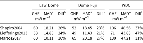
aMedian Absolute Deviation.
bPercentage of difference between the mean GHF and the MAD from the map using Eqn (12).
Notes For this study, the standard deviation values from the models are converted into MAD.
Implications
We have shown that ice-borehole temperature profiles can be used to estimate local GHF values and to discriminate between available GHF maps produced by geophysical models. Our approach could also be useful in assessing the location of potential ‘old’ ice core sites by verifying the required assumption of no melting at the bottom of the ice sheet. In the aim of finding sites that contain million-year-old ice, it is important that melting has not occurred at the base of the ice sheet in the past million years (Fischer and others, Reference Fischer2013; Liefferinge and Pattyn, Reference Liefferinge and Pattyn2013; Parrenin and others, Reference Parrenin2017; Karlsson and others, Reference Karlsson2018). Even if it is possible to identify the current presence of melt water at the ice/bedrock interface by using radio echo sounding (e.g. Pattyn, Reference Pattyn2010), understanding past subglacial conditions of the AIS is possible only by modelling past variations in ice-sheet basal temperature. In regions with negligible dissipative heating, which is a common characteristic of most ice core sites, the main factors that influence the basal temperature are accumulation rate, surface temperature, thickness of the ice sheet and GHF. Even with a temperature profile that is not complete, our model gives a range of likely GHF values. With a range of acceptable GHF produced by the model, the surface temperature history, the variation of ice thickness and the variation of accumulation rate through time, it is possible to produce a range of likely basal temperatures that a specific location could have experienced in the past. Then, it would be possible to assess if the basal temperature had reached the pressure melting point in the past.
Conclusion
Our model is able to assess the variation in GHF estimations from ice-borehole temperature profiles truncated at different depths. At our focus location near the top of Law Dome (DSS), our models suggest that only 57% of the available temperature profile is required to produce an acceptable GHF value (i.e. within 1 MAD of LD100 GHF median value). However, by comparing with Dome Fuji and WDC, which require as much as 80 and 90% of the available temperature profiles, respectively, for the same level of accuracy, we notice that several external factors have an impact on our estimations. First, the six assumptions used in the model, which was designed primarily for the DSS site, could have an impact on the model results for Dome Fuji and WDC, especially the assumption of no horizontal velocity. It is important to build a suitable model for each location. Additionally, depending on the thickness of the ice sheet and the accumulation rate, the temperature of the ice sheet could be affected by past glacial cycles. The WDC ice core site, which arguably does not meet the different assumptions of our model and where the ice sheet is >3000 m thick, produces GHF estimations with a more erratic behaviour when the profile is truncated than the other two locations because WDC seems to have the most complex relationship between temperature and depth.
Depending on the required application of the GHF estimation, we show that it is possible to use relatively shallow temperature profiles to produce satisfying results. At Law Dome, for a GHF value that is less than 10% different from the median GHF using the whole 1177 m, only 50% of the temperature profile is necessary. Comparison of our modelled GHF median and MAD values with those from Shapiro and Ritzwoller (Reference Shapiro and Ritzwoller2004), Liefferinge and Pattyn (Reference Liefferinge and Pattyn2013) and Martos and others (Reference Martos2017) shows that the percentage of the individual temperature profiles (compared to total profile depth available) required to discriminate between the models at the borehole locations are 42% at Law Dome, 60% at Dome Fuji and ≈45% at the WDC.
Finally, by producing a range of likelihood GHF values, our model could be used for other purposes like confirming the assumption that there was no melting at the base of the ice sheet in the past. The values in our method open up the opportunity for fairly accessible GHF estimations across wide areas of ice cover to enable more representative estimates and assess spatial variation, and for targeted use in regions of interest (e.g. old ice sites). Future direct observations of GHF are necessary to produce maps that will be able to represent the actual spatial variability of GHF and minimise the error on the estimations. The use of shallow ice-borehole temperature profiles, and the modelling approach outlined here could aid this process, avoiding the logistical challenges of drilling deep boreholes in ice and bedrock.
Acknowledgments
We thank the members of the ice-sheet group at IMAS, especially Adam Treverrow and Felicity McCormack, for reviewing and improving an earlier version of the manuscript. This research was supported under Australian Research Council's Special Research Initiative for Antarctic Gateway Partnership (Project ID SR140300001).


 Open access