


1. Introduction
Actuaries must understand the mortality characteristics of portfolios they work on, and a key goal of any model is that it must reflect reality. This has two facets. First, a model must not make assumptions that contradict the data. In particular, the analyst should not have to discard data because it is inconvenient for the model; a model should match the data, not the other way around. Second, a model should be capable of reproducing real-world features of the risk. As we will see, continuous-time methods have specific advantages over discrete-time models in both respects.
In their landmark paper, Forfar et al. (Reference Forfar, McCutcheon and Wilkie1988) considered three different metrics for modelling mortality: (i) the discrete-time probability of death, ${q_x}$
, (ii) the central mortality rate,
${q_x}$
, (ii) the central mortality rate, ${m_x}$
, and (iii) the continuous-time hazard rate,
${m_x}$
, and (iii) the continuous-time hazard rate, ${\mu _x}$
. Of the three,
${\mu _x}$
. Of the three, ${m_x}$
has fallen somewhat into disuse, in part because it does not arise as a parameter in a statistical model. The probability
${m_x}$
has fallen somewhat into disuse, in part because it does not arise as a parameter in a statistical model. The probability ${q_x}$
retains an important pedagogical role for students – there is nothing simpler than the idea of mortality viewed as a binomial trial over a fixed period like a year. However, this simplicity often collides with the messier reality of business processes. This paper explores some practical reasons why
${q_x}$
retains an important pedagogical role for students – there is nothing simpler than the idea of mortality viewed as a binomial trial over a fixed period like a year. However, this simplicity often collides with the messier reality of business processes. This paper explores some practical reasons why ${\mu _x}$
is usurping
${\mu _x}$
is usurping ${q_x}$
in actuarial work. The companion paper, Macdonald and Richards (Reference Macdonald and Richards2025), provides some theoretical underpinning.
${q_x}$
in actuarial work. The companion paper, Macdonald and Richards (Reference Macdonald and Richards2025), provides some theoretical underpinning.
The plan of the rest of this paper is as follows. In Section 2 we state assumptions and define some terms. Section 3 compares the ability of discrete- and continuous-time models to represent the data produced by various business processes. Section 4 looks at a variety of mortality features that require greater granularity than a one-year, discrete-time view of risk. Section 5 illustrates the greater flexibility with investigation period offered by continuous-time methods. Section 6 explores the analysis of competing decrements. Section 7 considers the uses of some non- and semi-parametric techniques for data-quality checking, while Section 8 discusses their application for real-time management information. Section 9 discusses the results and Section 10 concludes. Appendix A contains numerous case studies based on actual business experience. Appendix B details the difficulties that discrete-time models have in dealing with fractional periods of exposure. Appendix C considers the bias introduced when discarding data. Appendix D provides a primer in non- and semi-parametric methods for actuaries, while Appendix E outlines some features of grouped-count models.
2. Assumptions and Terminology
We assume that we are primarily interested in the analysis of mortality, although many of the comments apply to other decrements. Mortality is most naturally described in a continuous-time settingFootnote 1 . That said, the most granular measure of time recorded in an administration system is typically a calendar date. This means that “continuous time” is for practical purposes synonymous with “daily.” However, while an individual can die on any date, this information may not always be available for analysis – Case Study A.10 describes an example where only the month of death was available, while in Case Study A.17 only the year of death was available (see Appendix A). Where the date of death is not known exactly, deaths are said to be interval censored; the event is only known to have occurred between two points. In Case Study A.10, the interval is a calendar month, whereas in Case Study A.17 it is a year.
An event is an occurrence at a point in time that is of financial interest, such as a death or policy lapse. Other events are deemed irrelevantFootnote 2 . Events can occur in any order consistent with physical or procedural possibility, e.g. a pension-scheme member cannot retire after dying. Simultaneous events are ruled out by assumption. Note that there is a distinction between an event occurring and when (or if) that event is reported to the insurer or pension administrator; see the discussion of late-reported deaths in Section 4.3.
A discrete-time model for mortality assumes that the life in question exists at the start of a fixed period, such as one year, and is either alive ( $d = 0$
) or dead (
$d = 0$
) or dead ( $d = 1$
) at the end of this period. No other event is permitted, such as an earlier exit. No information is available on the time of the event during the fixed period; we only know whether the life died, not when. Discrete-time models are typically parameterized by
$d = 1$
) at the end of this period. No other event is permitted, such as an earlier exit. No information is available on the time of the event during the fixed period; we only know whether the life died, not when. Discrete-time models are typically parameterized by $q$
or
$q$
or ${q_x}$
. We will call such models “
${q_x}$
. We will call such models “ $q$
-type models.”
$q$
-type models.”
A continuous-time model for mortality assumes that the life in question is aged $x \ge 0$
at the start of observation and is observed for
$x \ge 0$
at the start of observation and is observed for $t \gt 0$
years. At age
$t \gt 0$
years. At age $x + t$
the life is either dead (
$x + t$
the life is either dead ( $d = 1$
) or was alive when last observed (
$d = 1$
) or was alive when last observed ( $d = 0$
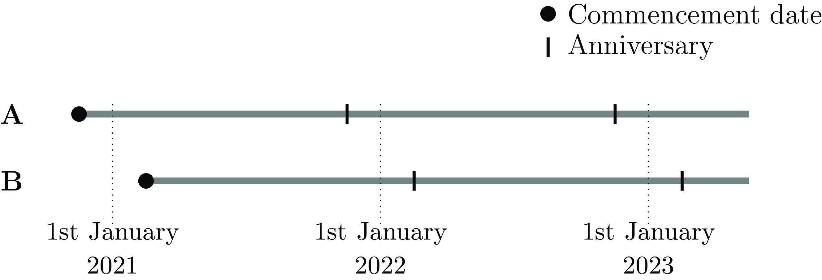
); see Cases A and B in Figure 1. If other events are accommodated by ceasing observation at age
$d = 0$
); see Cases A and B in Figure 1. If other events are accommodated by ceasing observation at age $x + t$
, then the observation is regarded as censored with respect to the decrement of interest, i.e. death. A crucial distinction from discrete-time models is that we know when the event of interest took place. Continuous-time models typically denote the risk by
$x + t$
, then the observation is regarded as censored with respect to the decrement of interest, i.e. death. A crucial distinction from discrete-time models is that we know when the event of interest took place. Continuous-time models typically denote the risk by $\mu $
or
$\mu $
or ${\mu _x}$
.
${\mu _x}$
. ${\mu _x}$
was known to actuaries as the force of mortality, and to engineers as the failure rate. However, we prefer the term hazard rate, as used by statisticians (Collett, Reference Collett2003, Section 1.3). We will refer to such models as “
${\mu _x}$
was known to actuaries as the force of mortality, and to engineers as the failure rate. However, we prefer the term hazard rate, as used by statisticians (Collett, Reference Collett2003, Section 1.3). We will refer to such models as “ $\mu $
-type models.”
$\mu $
-type models.”
Timelines for various annuitant cases with usable exposure time, $t$
, marked in grey. Case A is a survivor administered on the system from the annuity commencement date to the extract date. Case B is an annuity administered on the system from outset, but where death has occurred prior to the extract date. Case C represents an annuity administered on the system until either commutation, transfer to another system or transfer to another insurer. Cases D and E are annuities that were set up on another system or insurer at outset and subsequently transferred onto the current system. Cases with
$t$
, marked in grey. Case A is a survivor administered on the system from the annuity commencement date to the extract date. Case B is an annuity administered on the system from outset, but where death has occurred prior to the extract date. Case C represents an annuity administered on the system until either commutation, transfer to another system or transfer to another insurer. Cases D and E are annuities that were set up on another system or insurer at outset and subsequently transferred onto the current system. Cases with $d = 0$
are all right-censored with respect to mortality.
$d = 0$
are all right-censored with respect to mortality.
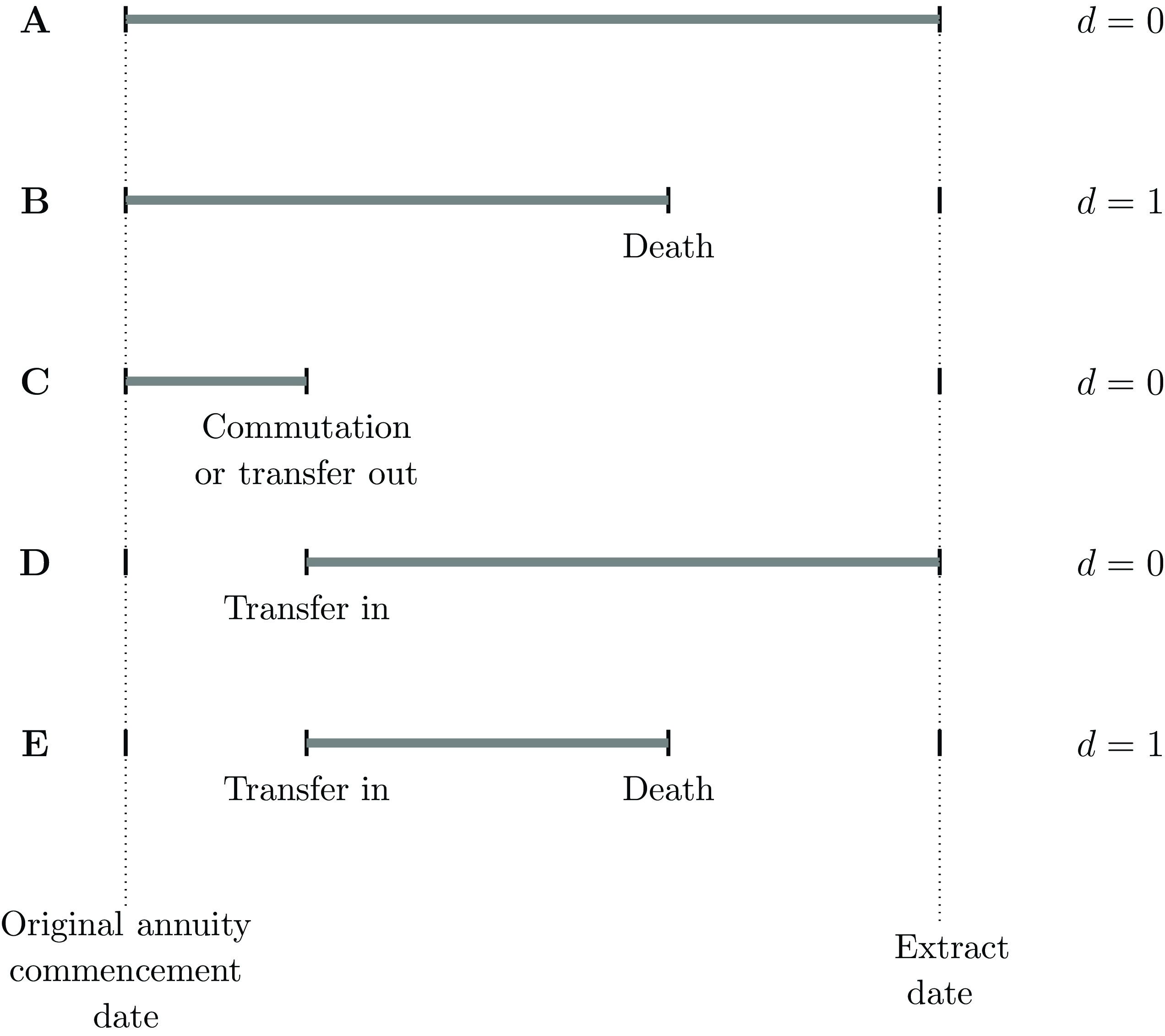
The most common type of censoring is where all that can be said is that death had not been reported at the last point of observation, known as right-censoring. Examples of right-censoring points include the date of extract, the date of transfer out or the date of trivial commutation; in each case, the life under observation was not reported to have died at the point of last observation. Cases A, C and D in Figure 1 are examples of right-censored observations. There are two sub-types of right-censoring: (i) “obligate” right-censoring, where observation ceases at a point in time known in advance, and (ii) random right-censoring, where observation ceases at a point in time not known in advance. The distinction becomes important when the analyst decides to discard data; see Appendix C.
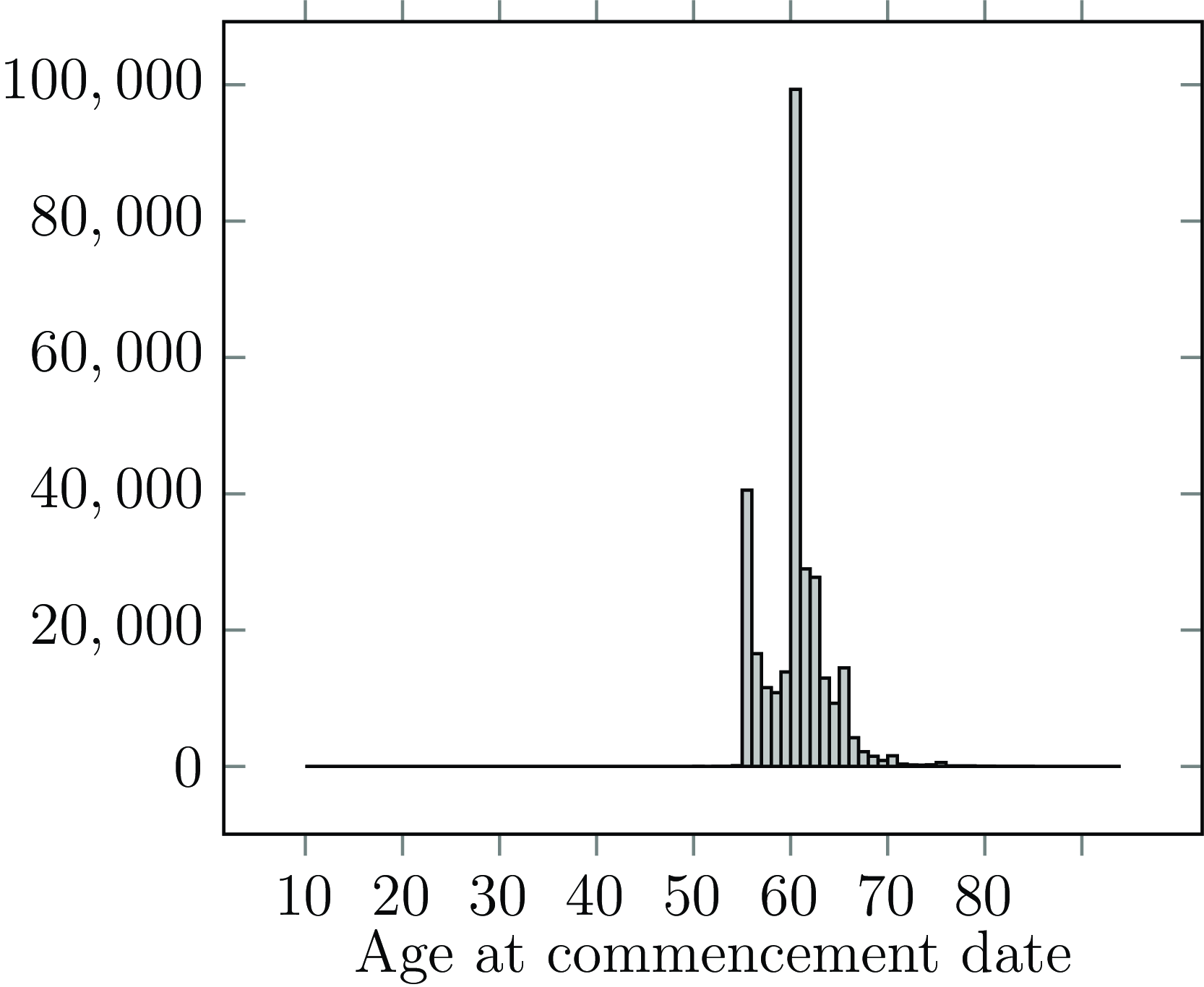
The start of an observation period for a life is qualitatively different from the end of the observation period. In actuarial work, most policyholders only become known to the portfolio well into their adult life; Figure 2 shows the distribution of age at commencement for annuities set up with a French insurer, where almost nobody enters observation before age 55 (an exception is shown in Figure A2). This is left truncation, where the mortality of those not entering observation is by definition unknown. Left truncation is a central feature of actuarial survival analysis, in contrast to, say, medical analysis (Collett, Reference Collett2003). Left truncation arises naturally, such as when a policy first commences or retirement commences (Section 3.2). However, left truncation can also be introduced by business processes (such as the system migrations discussed in Section 3.3) and deliberate analyst decisions (such as described in Section 5).
Histogram of age last birthday at annuity commencement date.
Source: 298,906 annuities for a French insurer.
We assume that we have data on individuals. If we have data on benefits or policies, we will first need to create records for individual lives through a process of deduplication; see Macdonald et al. (Reference Macdonald, Richards and Currie2018, Section 2.5). Deduplication is not merely a prerequisite for the independence assumption underlying statistical modelling, but it also results in a better understanding of risk and can even save money; see Case Study A.1 in Appendix A for an example. Note that having data on individual lives does not presuppose that we must model their risk individually, although this is desirable. However, extracting individual records does enable detailed validation and checking (Macdonald et al., Reference Macdonald, Richards and Currie2018, Sections 2.3 and 2.4).
The preceding descriptions of $q$
-type and
$q$
-type and $\mu $
-type models assume the modelling of individuals for simplicity. However, the analyst also has the option to model grouped counts by allocating individuals to groups and computing appropriate aggregate death counts and exposure measures; see Macdonald and Richards (Reference Macdonald and Richards2025), Appendix A, especially Figure 4, for the details of the splitting of the individual observations and assigning them to rate intervals. The advantages and disadvantages of grouped-count modelling are discussed in Macdonald et al. (Reference Macdonald, Richards and Currie2018, Section 1.7).
$\mu $
-type models assume the modelling of individuals for simplicity. However, the analyst also has the option to model grouped counts by allocating individuals to groups and computing appropriate aggregate death counts and exposure measures; see Macdonald and Richards (Reference Macdonald and Richards2025), Appendix A, especially Figure 4, for the details of the splitting of the individual observations and assigning them to rate intervals. The advantages and disadvantages of grouped-count modelling are discussed in Macdonald et al. (Reference Macdonald, Richards and Currie2018, Section 1.7).
Time periods are often expressed in years. A practical issue is that the difference between two dates is a number of days, but calendar years do not always have the same number of days. Macdonald et al. (Reference Macdonald, Richards and Currie2018, p.38) standardize by dividing the number of days between two dates by 365.242 to account for leap years (Richards (Reference Richards, Urban and Seidelman2012, Table 15.1) gives a value of 365.24219 days for the astronomical cycle for the year 2000).
One question is how to handle dates at the start and end of a period of time. We adopt a policy of assuming that an interval starts at mid-day on the start date and ends at mid-day on the end date. For example, this means that the interval from 1st-31st January 2024 is taken to be 30 days long ( $30 = 31 - 1$
) and not 31 days. This allows us to subdivide intervals without double-counting, e.g. the interval from 1st-16th January 2024 is 15 days long and the interval from 16th-31st January 2024 is 15 days long. Intervals that start and end on the same date have zero length and are excluded from analysis. A death at the end date is assumed to happen at mid-day. Thus, if the exposure period is 1st-31st January 2024 and
$30 = 31 - 1$
) and not 31 days. This allows us to subdivide intervals without double-counting, e.g. the interval from 1st-16th January 2024 is 15 days long and the interval from 16th-31st January 2024 is 15 days long. Intervals that start and end on the same date have zero length and are excluded from analysis. A death at the end date is assumed to happen at mid-day. Thus, if the exposure period is 1st-31st January 2024 and $d = 1$
, then we have 30 days of exposure terminated with a death.
$d = 1$
, then we have 30 days of exposure terminated with a death.
3. Reflecting Reality: Business Processes
A fundamental assumption of a $q$
-type model is that it is a Bernoulli trial, i.e. we observe each individual at the start and end of a complete year only. Otherwise, the complete year may not be interrupted by any right-censoring events, such as lapsing or the end of the investigation.
$q$
-type model is that it is a Bernoulli trial, i.e. we observe each individual at the start and end of a complete year only. Otherwise, the complete year may not be interrupted by any right-censoring events, such as lapsing or the end of the investigation.
Pensions and annuities in payment are nominally a single-decrement risk, i.e. the only way they are supposed to cease is through the death of the recipient. On the face of it, this matches the $q$
-type model in theory. However, in the following examples we will see that
$q$
-type model in theory. However, in the following examples we will see that $q$
-type models often do not match the reality of business practices, and that
$q$
-type models often do not match the reality of business practices, and that $\mu $
-type modelling is a more natural choice.
$\mu $
-type modelling is a more natural choice.
3.1. Bulk Transfers Out of a Portfolio
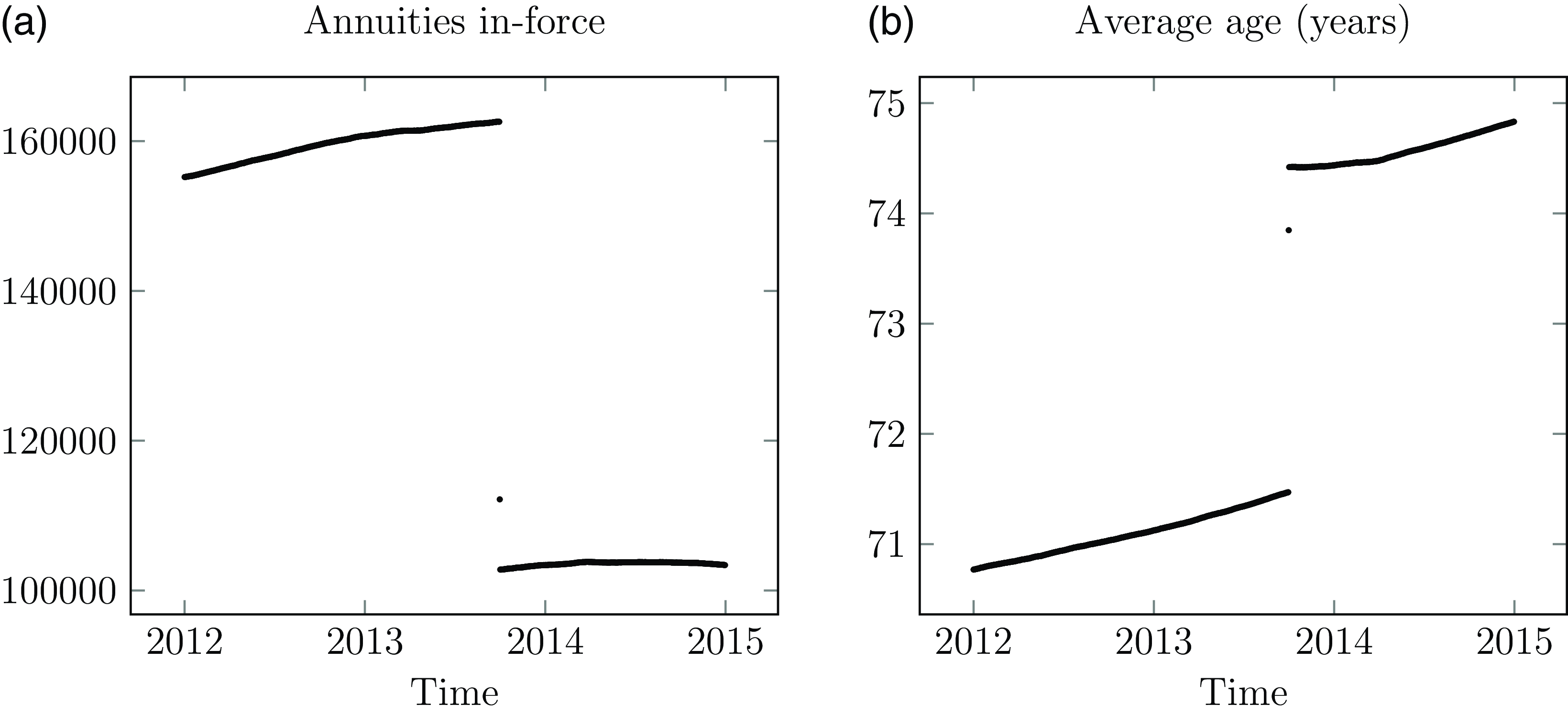
Portfolios can experience mid-year transfers out en masse. Examples include a transfer of annuities to another insurer, the purchase of buy-out annuities in a pension scheme or transfer to another administration system. Figure 3 shows an example for a UK annuity portfolio, where a large block of annuity contracts was moved to another insurer in a Part VII transfer (FSM, 2000, PartVII).
(a) Number of in-force annuities and (b) average age of in-force annuities at each date for a UK insurer. The discontinuities in late 2013 are caused by a transfer of liabilities to another insurer. New annuities are set up on any day, hence the seemingly continuous nature of the in-force annuity count at other times.
Source: Own calculations using experience data for all ages, January 2012–December 2014.
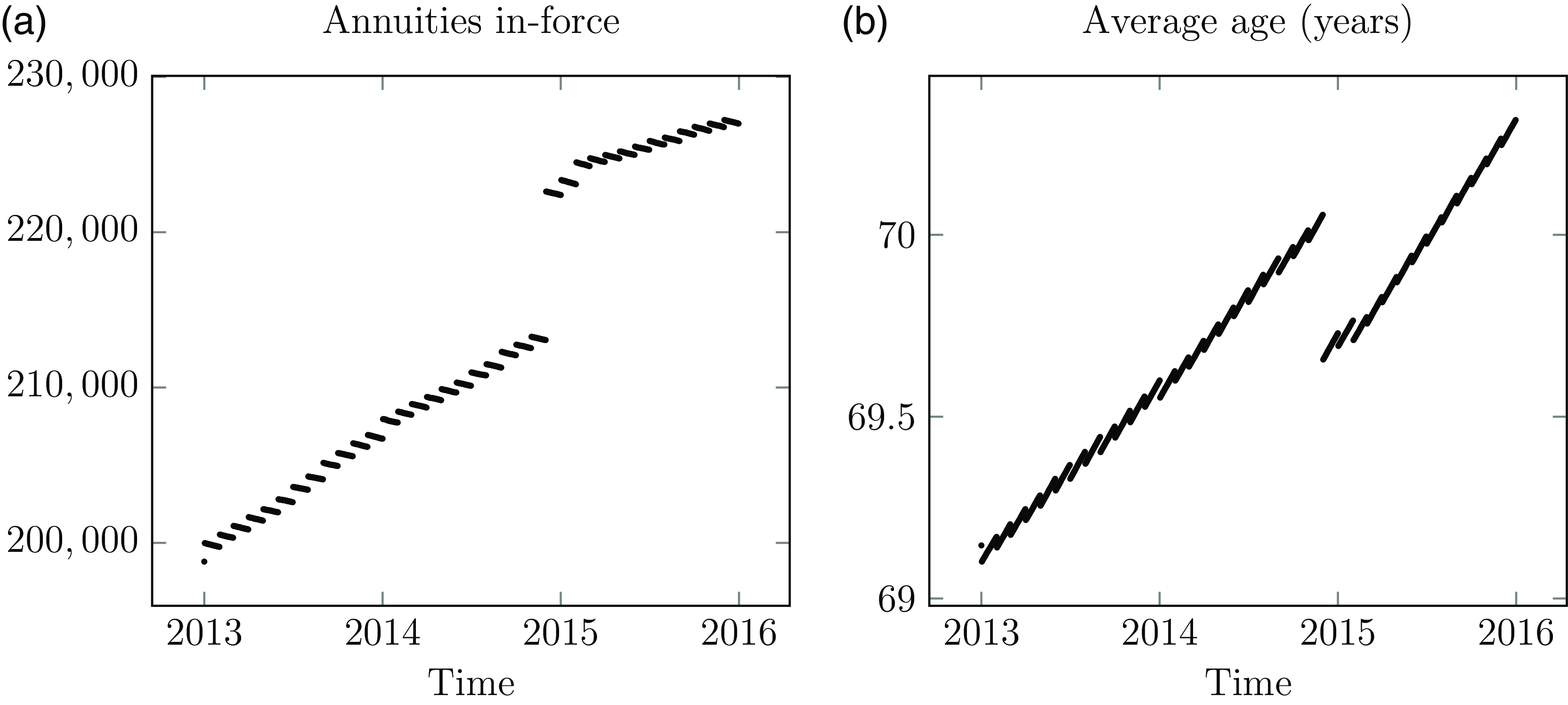
(a) Number of in-force annuities and (b) average age of in-force annuities at each date for a French insurer. The discontinuity in December 2014 was caused by a surge in new business. New annuities are set up on the first of the month, hence the stepped pattern of the annuity in-force count.
Source: Experience data for all ages, January 2013–December 2015.
Mid-year exits like in Figure 3(a) are a problem for $q$
-type models. They violate the assumption that there is no other possible event besides death or survival to the end of the year. In contrast, mid-year exits pose no problem for modelling in continuous time – the transfer out date is the date of last observation, and the indicator variable is set
$q$
-type models. They violate the assumption that there is no other possible event besides death or survival to the end of the year. In contrast, mid-year exits pose no problem for modelling in continuous time – the transfer out date is the date of last observation, and the indicator variable is set $d = 0$
to signify that the life was alive at that date. See Case C in Figure 1, and Case Studies A.1 and A.4 in Appendix A.
$d = 0$
to signify that the life was alive at that date. See Case C in Figure 1, and Case Studies A.1 and A.4 in Appendix A.
3.2. New Business
In addition to mid-year exits, most pension schemes and annuity portfolios also add new liabilities. These can be due to new retirements or spouse’s annuities set up on death of the first life. It is also possible to have a mass influx of new pensions, such as a pension scheme seeing a wave of early retirements due to corporate restructuring. Figure 4 shows an annuity portfolio where new cases are added at the start of each month and where there was a surge in new business in December 2014.
If an analyst is modelling $q$
-type rates aligned on calendar years, then any new records added during the year require special handling because a complete year of exposure is not possible. In contrast, all new business records can be used in a continuous-time model in the same way as in-force records; see Case Study A.8 in Appendix A.
$q$
-type rates aligned on calendar years, then any new records added during the year require special handling because a complete year of exposure is not possible. In contrast, all new business records can be used in a continuous-time model in the same way as in-force records; see Case Study A.8 in Appendix A.
3.3. Bulk Transfers into a Portfolio
For every bulk transfer out of one portfolio in Section 3.1 there will be a corresponding bulk transfer in to another portfolio. Examples include an insurer receiving a Part VII transfer, an insurer writing a large bulk annuity, or an administration system receiving migrated records from another administration system. This is like the new business in Section 3.2, but with the added complication that the receiving system will be missing deaths between annuity commencement and the transfer-in date. This is of course a challenge for $q$
-type models in the same way as for new business, but it is not a problem for continuous-time methods – see Cases D and E in Figure 1 and Case Study A.13 in Appendix A.
$q$
-type models in the same way as for new business, but it is not a problem for continuous-time methods – see Cases D and E in Figure 1 and Case Study A.13 in Appendix A.
3.4. Commutations and Temporary Pensions
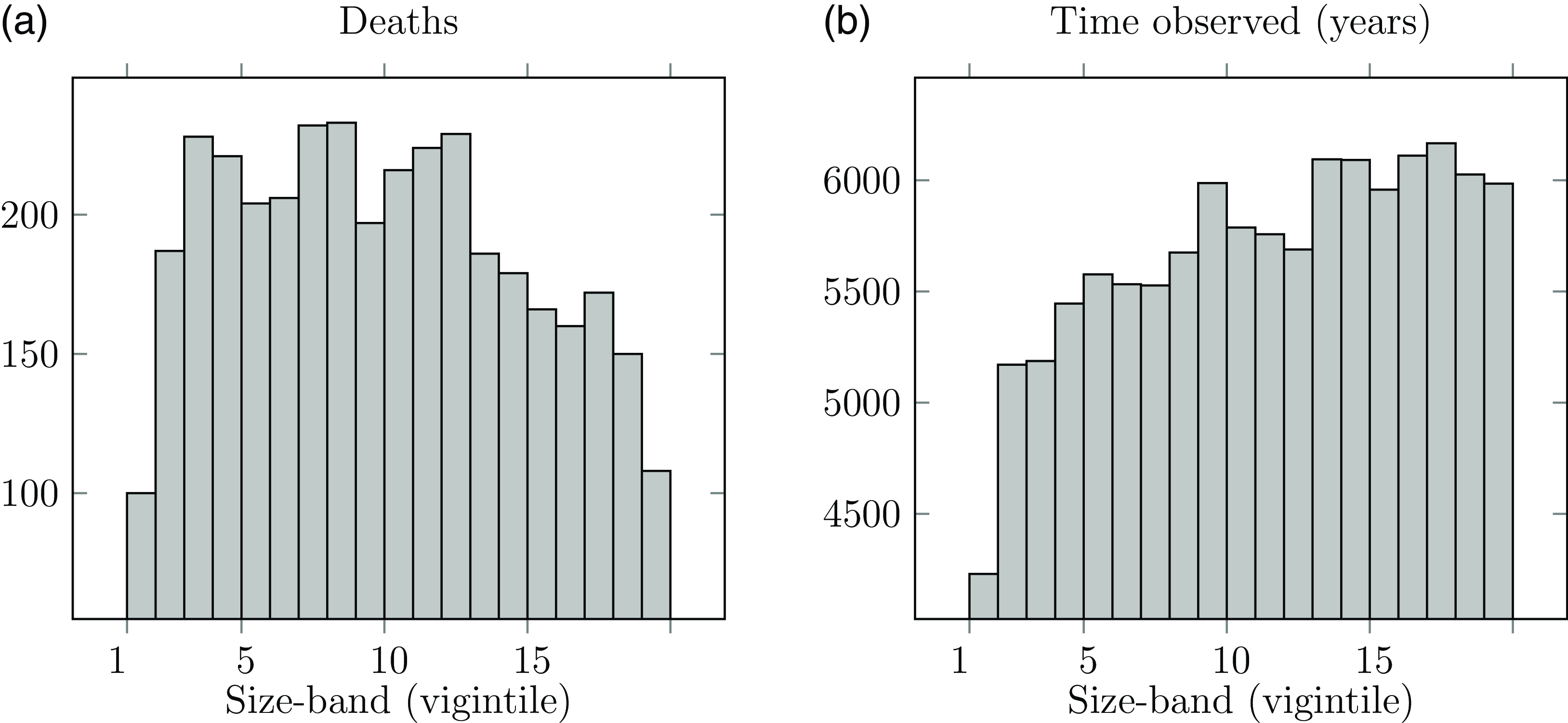
Even if a portfolio experiences no mass transfer out, it is still possible for individual liabilities to cease for a reason other than death. In the UK, pension benefits below a certain size can be commuted into a taxable lump sum. Administration expenses are largely fixed in nature, so the facility to commute small pensions saves disproportionate costs. However, this again means that the pension ceases for a reason other than the death of the recipient. Figure 5 shows the impact of this – although the number of lives in each size-band is the same, the time lived is much reduced for the smallest size-band due to non-death early exits. The number of observed deaths is correspondingly much reduced, as post-commutation deaths are of course unknown to the insurer.
(a) Deaths and (b) time observed in each pension size-band, showing the reduced exposure for the smallest pensions.
Source: Own calculations using experience data for Scottish pension scheme, ages 50–105, years 2000–2009. Pensioner records were sorted by pension size and grouped into twenty bands of equal numbers of lives (vigintiles). Size-band 1 represents the 5% of pensioners receiving the lowest pensions, while size-band 20 represents the 5% of pensioners receiving the largest amounts.
There are other ways for pensions to cease for a reason other than death. In Richards et al. (Reference Richards, Kaufhold and Rosenbusch2013) a multi-employer pension administrator in Germany had (i) temporary widow(er) pensions, (ii) widow(er) pensions ceasing on remarriage and (iii) disability pensions ceasing due to a return to work. In the Chilean national pension system, spouses’ pensions also cease upon remarriage. Some UK pension schemes grant pensions to “surviving adults” that can be terminated on remarriage or cohabitation with another person (TPS, 2010, 94(6)).
Commutations and temporary pensions pose a problem for $q$
-style models of mortality. One option is to exclude such cases, but this depends on them being clearly identified as such; see Case Study A.9 in Appendix A. Another issue is the need to exclude any corresponding deaths – trivial commutations are not always processed immediately, which means it is possible for a commutation-eligible pensioner to die first. Appendix C shows how discarding lapsed cases leads to a bias in mortality estimation. Discarding such data is therefore to be avoided.
$q$
-style models of mortality. One option is to exclude such cases, but this depends on them being clearly identified as such; see Case Study A.9 in Appendix A. Another issue is the need to exclude any corresponding deaths – trivial commutations are not always processed immediately, which means it is possible for a commutation-eligible pensioner to die first. Appendix C shows how discarding lapsed cases leads to a bias in mortality estimation. Discarding such data is therefore to be avoided.
In contrast, commutations and temporary pensions do not pose any kind of problem for models in continuous time – the commutation date is the date of last observation, and the indicator variable is set $d = 0$
to signify that the life was alive at that date. See Case C in Figure 1 and Case Studies A.1 and A.4 in Appendix A.
$d = 0$
to signify that the life was alive at that date. See Case C in Figure 1 and Case Studies A.1 and A.4 in Appendix A.
3.5. Representation of Data
In all the foregoing examples, non-death exits and mid-year entries are handled more easily by modelling in continuous time. This allows for simpler data preparation and corresponds more closely to the realities of the business processes than $q$
-type models. To illustrate, we assume that we have a data extract from a pension or annuity administration system. For each record we calculate the data pair
$q$
-type models. To illustrate, we assume that we have a data extract from a pension or annuity administration system. For each record we calculate the data pair $\left\{ {{d_i},{t_i}} \right\}$
as follows.
$\left\{ {{d_i},{t_i}} \right\}$
as follows. ${t_i}$
is the real-valued time observed in years between the on-risk date and the off-risk date. The on-risk date is the latest of: (i) the annuity commencement date, and (ii) the transfer-in date (if any). If the transfer-in date is not known exactly, a suitable proxy date can be used, such as the date of first payment made on the system; see Case Study A.13 in Appendix A. The off-risk date is the earliest of: (i) the date of extract, (ii) the date of death (if dead), (iii) the date of commutation (if commuted), and (iv) the date of transfer out (if any). If the transfer-out date is not known exactly, a suitable proxy can be used, such as the date of last payment made on the system; see Case Study A.4 in Appendix A. The indicator variable is set
${t_i}$
is the real-valued time observed in years between the on-risk date and the off-risk date. The on-risk date is the latest of: (i) the annuity commencement date, and (ii) the transfer-in date (if any). If the transfer-in date is not known exactly, a suitable proxy date can be used, such as the date of first payment made on the system; see Case Study A.13 in Appendix A. The off-risk date is the earliest of: (i) the date of extract, (ii) the date of death (if dead), (iii) the date of commutation (if commuted), and (iv) the date of transfer out (if any). If the transfer-out date is not known exactly, a suitable proxy can be used, such as the date of last payment made on the system; see Case Study A.4 in Appendix A. The indicator variable is set ${d_i} = 1$
if the off-risk date is the date of death and
${d_i} = 1$
if the off-risk date is the date of death and ${d_i} = 0$
otherwise. This is depicted graphically in Figure 1.
${d_i} = 0$
otherwise. This is depicted graphically in Figure 1.
Macdonald et al. (Reference Macdonald, Richards and Currie2018, Section 2.9.1) give an expanded consideration to include analyst-specified limits, such as minimum and maximum ages, modelling start and end dates and rules for excluding suspicious records. All of these are more easily handled in $\mu $
-type models than with
$\mu $
-type models than with $q$
-type models.
$q$
-type models.
4. Reflecting Reality: Risk Features $q$
-type methods are by definition unable to model mortality phenomena that take place over a shorter time frame than the fixed period they span. In contrast, continuous-time methods can better reflect rapidly changing phenomena, as demonstrated in the following sub-sections.
$q$
-type methods are by definition unable to model mortality phenomena that take place over a shorter time frame than the fixed period they span. In contrast, continuous-time methods can better reflect rapidly changing phenomena, as demonstrated in the following sub-sections.
4.1. Mortality Shocks
The Covid-19 pandemic (The Novel Coronavirus Pneumonia Emergency Response Epidemiology Team, 2020) produced intense spikes in mortality in a number of countries. This is reflected in the portfolio data that actuaries analyse; see the examples for annuity portfolios in France, the UK and the USA in Richards (Reference Richards2022b). The first Covid-19 shock in the UK was in April & May 2020, and the intensity of this two-month mortality shock cannot be captured with annual or even quarterly $q$
-type rates. In contrast, continuous-time models can reveal rich detail. Figure 6 shows an example, where the first Covid-19 shock is detected in April & May 2020 with seasonal variation in the years beforehand. Underlying Figure 6 is a
$q$
-type rates. In contrast, continuous-time models can reveal rich detail. Figure 6 shows an example, where the first Covid-19 shock is detected in April & May 2020 with seasonal variation in the years beforehand. Underlying Figure 6 is a $B$
-spline basis with knots at half-year intervals to pick up the substantial seasonal variation. In addition, a priori knowledge of population mortality shocks led to the addition of further
$B$
-spline basis with knots at half-year intervals to pick up the substantial seasonal variation. In addition, a priori knowledge of population mortality shocks led to the addition of further $B$
-spline knots in the first half of 2020, thus giving a basis of varying flexibility over time (there is no requirement for a
$B$
-spline knots in the first half of 2020, thus giving a basis of varying flexibility over time (there is no requirement for a $B$
-spline basis to always have equally spaced knots; see Kaishev et al. (Reference Kaishev, Dimitrova, Haberman and Verrall2016)). The result is a model for
$B$
-spline basis to always have equally spaced knots; see Kaishev et al. (Reference Kaishev, Dimitrova, Haberman and Verrall2016)). The result is a model for ${\mu _x}$
that allows mortality to vary smoothly over time, with periods of faster and slower change. Such detail is impossible with an annual
${\mu _x}$
that allows mortality to vary smoothly over time, with periods of faster and slower change. Such detail is impossible with an annual $q$
-type model.
$q$
-type model.
Mortality level over time for a UK annuity portfolio, where modelling in continuous time allows rich detail to be identified. The mortality level is standardized at 1 in October 2019.
Source: Richards (Reference Richards2022c).
4.2. Period Effects and Selection
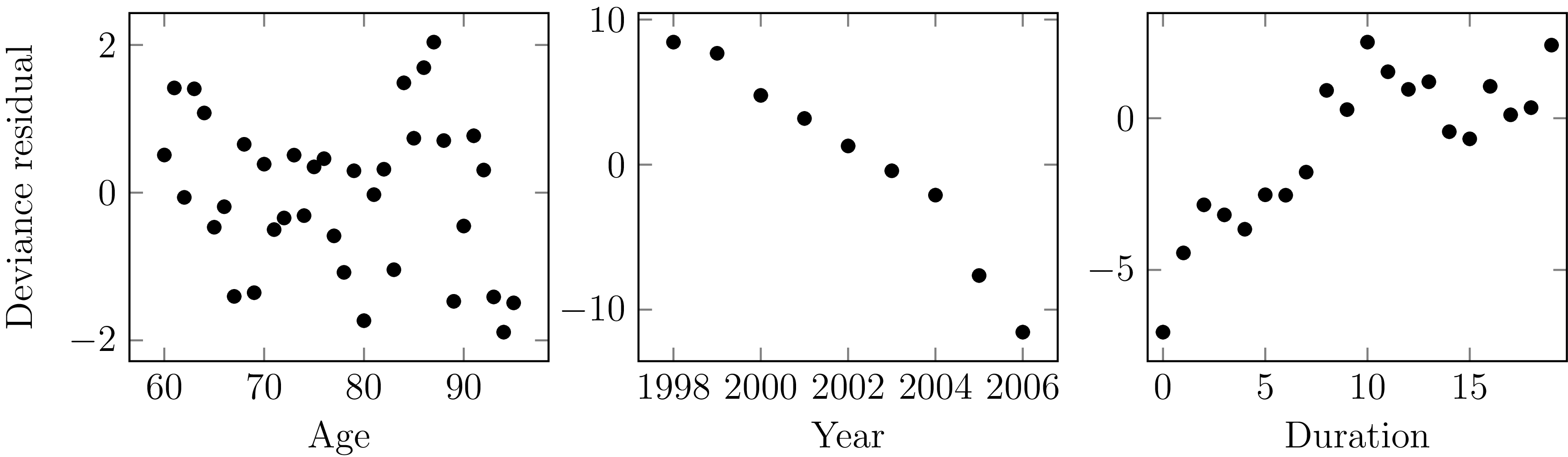
Figure 7 shows the deviance residuals (McCullagh and Nelder, Reference McCullagh and Nelder1989, Section 2.4.3) for a second portfolio of UK annuities. The model includes age and sex, and the random pattern of residuals by age suggests that the model is an acceptable fit for age-related mortality. However, the non-random patterns of residuals in time and duration suggest that it is also important to allow for both period effects and selection effects.
Deviance residuals by age, year and duration since commencement. The systematic pattern of residuals in the centre and right panels show that both time and duration are important risk factors for mortality, and should both be included in a model.
Source: own calculations for model for age and sex for second UK annuity portfolio, ages 60–95, years 1998–2006.
A drawback of a one-year $q$
-type model is that it is limited in how it can handle time-varying risk, especially when there are two or more time dimensions. This is due to the requirement to align the one-year intervals, as shown in Figure 8 for period effects and duration effects. This limitation of
$q$
-type model is that it is limited in how it can handle time-varying risk, especially when there are two or more time dimensions. This is due to the requirement to align the one-year intervals, as shown in Figure 8 for period effects and duration effects. This limitation of $q$
-type models improves a little if one of those risk factors is handled continuously (usually age). To see this, assume for simplicity that the basic mortality model is parametric, for example
$q$
-type models improves a little if one of those risk factors is handled continuously (usually age). To see this, assume for simplicity that the basic mortality model is parametric, for example ${q_x} = {e^{\alpha + \beta x}}/\left( {1 + {e^{\alpha + \beta x}}} \right)$
or
${q_x} = {e^{\alpha + \beta x}}/\left( {1 + {e^{\alpha + \beta x}}} \right)$
or ${\mu _x} = {e^{\alpha + \beta x}}$
. In each case we have a function defined for any real age,
${\mu _x} = {e^{\alpha + \beta x}}$
. In each case we have a function defined for any real age, $x$
, not just integer ages. We can also align the period effects on the calendar years, say by assuming that
$x$
, not just integer ages. We can also align the period effects on the calendar years, say by assuming that $\alpha $
is a function of calendar time, for example piecewise constant on calendar years. Since we have a function for mortality at any real age,
$\alpha $
is a function of calendar time, for example piecewise constant on calendar years. Since we have a function for mortality at any real age, $x$
, the fact that lives are at different ages during each year is not an issue for either the
$x$
, the fact that lives are at different ages during each year is not an issue for either the ${q_x}$
or the
${q_x}$
or the ${\mu _x}$
model.
${\mu _x}$
model.
When benefits can start at any point during the year, ${q_x}$
models can either include annual period effects or selection effects, but not both. For example, a period effect for 2021 requires a full year of exposure for survivors, so only Case A can contribute. However, the splitting of the exposure at annual boundaries means that different curtate durations are exposed, thus excluding the modelling of selection effects as well. The converse also applies.
${q_x}$
models can either include annual period effects or selection effects, but not both. For example, a period effect for 2021 requires a full year of exposure for survivors, so only Case A can contribute. However, the splitting of the exposure at annual boundaries means that different curtate durations are exposed, thus excluding the modelling of selection effects as well. The converse also applies.
However, how can the ${q_x}$
model accommodate selection effects for annuities commencing in the middle of the year? A one-year interval can either be aligned for annual period effects, or it can be aligned for selection effects, but it cannot be aligned for both. This is shown in Figure 8. In contrast, the
${q_x}$
model accommodate selection effects for annuities commencing in the middle of the year? A one-year interval can either be aligned for annual period effects, or it can be aligned for selection effects, but it cannot be aligned for both. This is shown in Figure 8. In contrast, the ${\mu _x}$
model can simultaneously model period and duration effects without such restriction. Of course, one could reduce the period covered by the
${\mu _x}$
model can simultaneously model period and duration effects without such restriction. Of course, one could reduce the period covered by the ${q_x}$
model to, say quarter-years. But if the answer is to reduce the fixed period covered by a
${q_x}$
model to, say quarter-years. But if the answer is to reduce the fixed period covered by a $q$
-type model, why not go all the way and reduce the interval to daily modelling?
$q$
-type model, why not go all the way and reduce the interval to daily modelling?
The problem of multivariate time scales is covered in detail in Andersen et al. (Reference Andersen, Borgan, Gill and Keiding1993), Chapter X. See also Case Study A.8 in Appendix A.
4.3. Occurred-but-not-Reported (OBNR) Deaths
One other useful aspect of continuous-time analysis is the ability to examine delays in the reporting of deaths. Lawless (Reference Lawless1994) describes this as the problem of occurred-but-not-reported (OBNR) events, and Kalbfleisch and Lawless (Reference Kalbfleisch and Lawless1991) consider parametric models for estimating the distribution of delays. Section D.5 in Appendix D describes the calculation of a semi-parametric estimator of the portfolio-level hazard in continuous time. Assume that we have two estimates of the mortality hazard at the same point in time $y + t$
. These two estimates are labelled
$y + t$
. These two estimates are labelled ${\hat \mu _y}\left( {t,{u_1}} \right)$
and
${\hat \mu _y}\left( {t,{u_1}} \right)$
and ${\hat \mu _y}\left( {t,{u_2}} \right)$
, and they differ only in that they have been calculated using data extracts taken at two different times
${\hat \mu _y}\left( {t,{u_2}} \right)$
, and they differ only in that they have been calculated using data extracts taken at two different times ${u_1} \lt {u_2}$
. Then
${u_1} \lt {u_2}$
. Then ${\hat \mu _y}\left( {t,{u_1}} \right)$
will be more affected by delays in the reporting of deaths than
${\hat \mu _y}\left( {t,{u_1}} \right)$
will be more affected by delays in the reporting of deaths than ${\hat \mu _y}\left( {t,{u_2}} \right)$
, with the effect decreasing the further
${\hat \mu _y}\left( {t,{u_2}} \right)$
, with the effect decreasing the further $y + t$
lies before
$y + t$
lies before ${u_1}$
. Figure 9 shows the ratio of
${u_1}$
. Figure 9 shows the ratio of ${\hat \mu _y}\left( {t,{u_1}} \right)/{\hat \mu _y}\left( {t,{u_2}} \right)$
as an estimate of the proportion of deaths that have not been reported. The two portfolios have minimal OBNR cases half a year or more before time
${\hat \mu _y}\left( {t,{u_1}} \right)/{\hat \mu _y}\left( {t,{u_2}} \right)$
as an estimate of the proportion of deaths that have not been reported. The two portfolios have minimal OBNR cases half a year or more before time ${u_1}$
, but have very different OBNR rates in the handful of months leading up to the extract. This level of insight is not possible with annual
${u_1}$
, but have very different OBNR rates in the handful of months leading up to the extract. This level of insight is not possible with annual $q$
-type analysis.
$q$
-type analysis.
Estimated proportion of deaths reported for annuity portfolios in France and UK. The horizontal axis is reversed, as it measures the time before the first extract at calendar time ${u_1}$
.
${u_1}$
.
Source: Richards (Reference Richards2022b, Section 4).
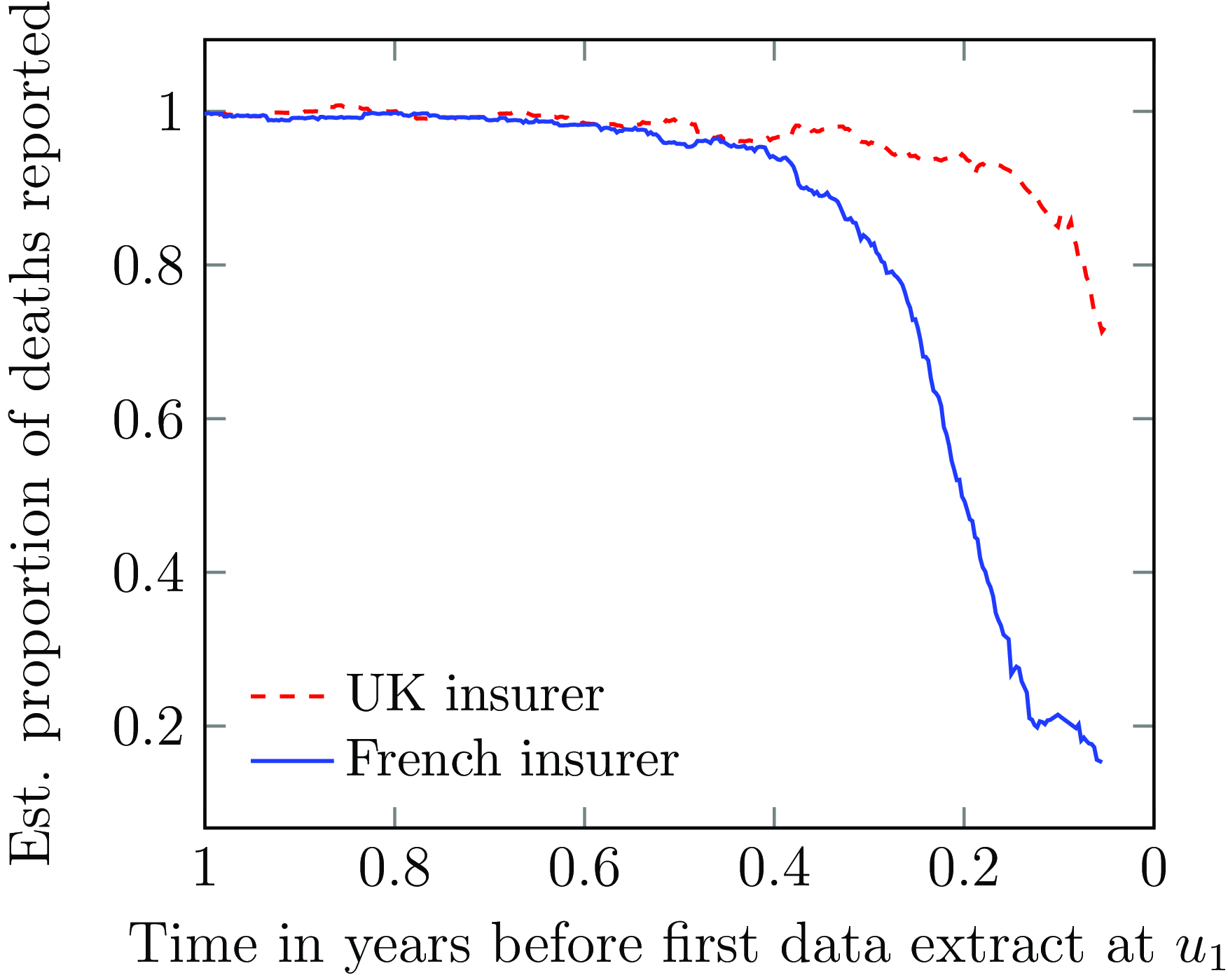
Continuous-time methods go further than the identification of reporting delays in Figure 9. Including a period affected by OBNR deaths will naturally tend to under-state mortality levels, which is one reason to discard the exposure period immediately prior to the extract date; Figure 9 suggests that six months should be discarded for the French annuity portfolio and three months for the UK one. However, continuous-time models make it possible to model these OBNR deaths and thus use the full experience data, even up to the date of extract itself. This OBNR allowance can be either parametric (Richards, Reference Richards2022b, Section 5) or semi-parametric (Richards, Reference Richards2022c, Section 10). Richards (Reference Richards2022b, Section 7) showed how the use of daily data and continuous-time methods allowed the “nowcasting” of current mortality affected by late-reported deaths. These sorts of techniques are not possible with annual $q$
-type approaches. See also Case Study A.15 in Appendix A.
$q$
-type approaches. See also Case Study A.15 in Appendix A.
4.4. Season
Annual $q$
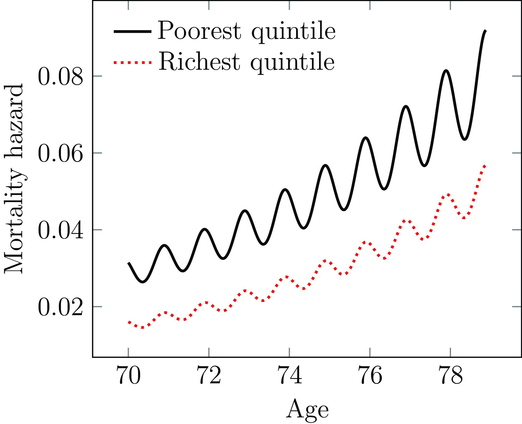
-type rates are by definition unable to model the seasonal variation shown in Figure 10. The mortality hazard rises overall as the lives age, but with fluctuations as the lives pass through the seasons of each year. The amplitude of these fluctuations grows larger with increasing age.
$q$
-type rates are by definition unable to model the seasonal variation shown in Figure 10. The mortality hazard rises overall as the lives age, but with fluctuations as the lives pass through the seasons of each year. The amplitude of these fluctuations grows larger with increasing age.
As a periodic factor, season has the unusual distinction of being both highly statistically significant in explaining mortality variation, and yet of low financial significance for long-term business (Richards, Reference Richards2020, Section 9). Nevertheless, accounting for seasonality can be useful in separating out the impact of pandemic shocks, and can help quantify the extent to which a heavy winter flu experience is unusual. Seasonal modelling has applications for public-policy work, such as the observation that poorer annuitants not only have higher mortality, but also experience stronger seasonal variation, as shown in Figure 10. Models of seasonal variation can also be useful in commercial situations, such as Case Studies A.5, A.7 and A.12 in Appendix A.
Modelled cohort mortality hazard for males initially aged 70 at 1st January by selected income quintile.
Source: model calibrated to mortality experience of large UK pension scheme in Richards et al. (Reference Richards, Ramonat, Vesper and Kleinow2020).
5. Investigation Period
The investigation period will be set by the analyst, and there may be specific organizational policies for this. In setting the investigation period, the analyst needs to balance the benefits of statistical power (from using a longer period) against relevance (such as when mortality levels have been falling or the portfolio mix is rapidly changing); see Benjamin and Pollard (Reference Benjamin and Pollard1986), page 49. For example, ONS (2024) use population experience data over a three-year period to create the UK National Life Tables, while some life offices have a policy of using five-year period to set bases. Other investigations use longer periods of exposure still.
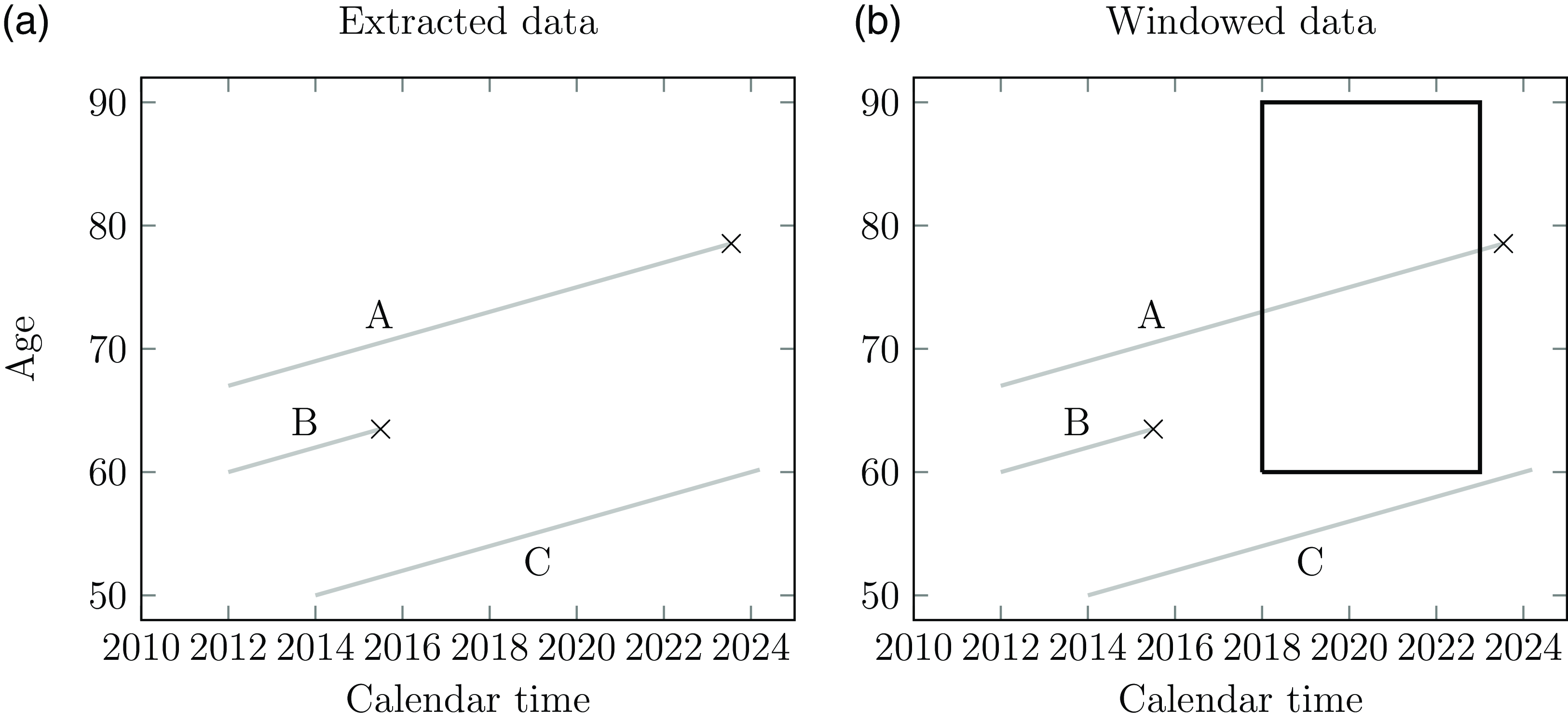
Specifying an investigation window causes additional left truncation and right-censoring, as shown in Figure 11; in addition to the life only becoming known to the insurer at an adult age at policy outset (standard left truncation) the analyst further discards the experience from policy outset to the start of the investigation window. Case Study A.18 in Appendix A concerns an annuity portfolio with uninterrupted experience data on the same administration system since outset. Despite the availability of decades of experience, the analyst would most likely only use the more recent data due to reasons of relevance. However, the length of the investigation period may also be limited by the data itself – Case Studies A.5 and A.7 in Appendix A are examples where the analyst has no scope for using a five-year investigation period.
An analyst wants to fit a Gompertz model of mortality to the experience between ages 60–90 over the period 1st January 2018–1st January 2023. An extract is taken of the data on 14th March 2024 and some specimen cases are shown in this Lexis diagram with exposure times in grey and deaths are marked with $ \times $
. (a) Raw experience data and (b) experience data within the analyst’s window superimposed. Individual A died on 20th July 2023, but is right-censored at the end of the investigation period and so is regarded as alive in the analysis. Individual A’s exposure time to the left of the window is also left-truncated. Individual B died before the investigation window opened and is excluded from the analysis. Individual C is also excluded from the analysis because they never reach the age range within the investigation period.
$ \times $
. (a) Raw experience data and (b) experience data within the analyst’s window superimposed. Individual A died on 20th July 2023, but is right-censored at the end of the investigation period and so is regarded as alive in the analysis. Individual A’s exposure time to the left of the window is also left-truncated. Individual B died before the investigation window opened and is excluded from the analysis. Individual C is also excluded from the analysis because they never reach the age range within the investigation period.
Most investigation periods also span a whole number of years, in part to balance out the seasonal fluctuations in mortality; see Figure 10 and years 2016–2019 in Figure 6. However, if a model includes an explicit seasonal term (Richards et al., Reference Richards, Ramonat, Vesper and Kleinow2020), then there is no need to worry about any bias caused by unbalanced numbers of summers and winters. This permits $\mu $
-type models to have an investigation period of a non-integer number of years if a seasonal component is included; see Case Studies A.5 and A.7 in Appendix A.
$\mu $
-type models to have an investigation period of a non-integer number of years if a seasonal component is included; see Case Studies A.5 and A.7 in Appendix A.
The ability to use fractional numbers of years in an investigation extends particularly to transactions such as bulk annuities. Pension schemes in the UK sometimes change administrators, which invariably leads to the loss of mortality data prior to the switchover. If a pension scheme can only supply 2.5 years of mortality experience, then the insurer will not want throw away a fifth of the information just because a GLM for ${q_x}$
can only use whole periods (although a
${q_x}$
can only use whole periods (although a $q$
-type model is still possible if one does not use a GLM; see Appendix B). Any concerns about delays in reporting of deaths can be addressed in a
$q$
-type model is still possible if one does not use a GLM; see Appendix B). Any concerns about delays in reporting of deaths can be addressed in a $\mu $
-type model by including an explicit occurred-but-not-reported (OBNR) term; see Richards (Reference Richards2022b), Section 5.
$\mu $
-type model by including an explicit occurred-but-not-reported (OBNR) term; see Richards (Reference Richards2022b), Section 5.
At the time of writing, most portfolios will still have recent mortality experience affected by Covid-19; see the spike in mortality in April and May 2020 in Figure 6. $\mu $
-type models can allow for such spikes in the experience (Richards, Reference Richards2022c) in a way that
$\mu $
-type models can allow for such spikes in the experience (Richards, Reference Richards2022c) in a way that $q$
-type models cannot. However, another alternative to avoiding bias might be to exclude the affected period, although this presupposes that the Covid-affected experience is an additive outlier with no relevance to later mortality. For a
$q$
-type models cannot. However, another alternative to avoiding bias might be to exclude the affected period, although this presupposes that the Covid-affected experience is an additive outlier with no relevance to later mortality. For a ${q_x}$
GLM this involves discarding an entire year’s worth of data, despite the fact that the shock in Figure 6 only lasts around two months (although, as before, a
${q_x}$
GLM this involves discarding an entire year’s worth of data, despite the fact that the shock in Figure 6 only lasts around two months (although, as before, a $q$
-type model is still possible if one does not use a GLM). In contrast,
$q$
-type model is still possible if one does not use a GLM). In contrast, $\mu $
-type models can more easily handle the ad hoc exclusion of short periods of experience, if the analyst feels that this is truly necessary. Macdonald and Richards (Reference Macdonald and Richards2025), Section 4.3 show how both left truncation and right-censoring can be handled by setting an exposure indicator function,
$\mu $
-type models can more easily handle the ad hoc exclusion of short periods of experience, if the analyst feels that this is truly necessary. Macdonald and Richards (Reference Macdonald and Richards2025), Section 4.3 show how both left truncation and right-censoring can be handled by setting an exposure indicator function, $Y\left( x \right)$
, to zero to “switch off” the contribution of exposure time and observed deaths to estimation.
$Y\left( x \right)$
, to zero to “switch off” the contribution of exposure time and observed deaths to estimation. $Y\left( x \right)$
is a multiplier of
$Y\left( x \right)$
is a multiplier of ${\mu _x}$
, and to exclude the contribution of Covid-affected experience, one could also set
${\mu _x}$
, and to exclude the contribution of Covid-affected experience, one could also set $Y\left( x \right) = 0$
for the period of any mortality shocks.
$Y\left( x \right) = 0$
for the period of any mortality shocks.
6. Competing Decrements
A limitation of $q$
-type models is that they assume that only two events are possible: survival to the end of the observation interval, or death during it. Even with notionally single-decrement business like pensions or annuities in payment, Section 3 shows that the business reality is that there are often other decrements like administrative transfers or trivial commutations.
$q$
-type models is that they assume that only two events are possible: survival to the end of the observation interval, or death during it. Even with notionally single-decrement business like pensions or annuities in payment, Section 3 shows that the business reality is that there are often other decrements like administrative transfers or trivial commutations.
However, the situation for $q$
-type models becomes worse with classes of business that have multiple modes of exit by design. Consider the data in Case Study A.32, where there are two decrements of interest: death and entry into long-term care.
$q$
-type models becomes worse with classes of business that have multiple modes of exit by design. Consider the data in Case Study A.32, where there are two decrements of interest: death and entry into long-term care. $n = 42$
lives start exposure at age 88, with
$n = 42$
lives start exposure at age 88, with ${d^{{\rm{mort}}}} = 5$
dying and
${d^{{\rm{mort}}}} = 5$
dying and ${d^{{\rm{care}}}} = 3$
entering long-term care before reaching age 89. Due to these exits and other censoring points there are
${d^{{\rm{care}}}} = 3$
entering long-term care before reaching age 89. Due to these exits and other censoring points there are ${E^c} = 36.9039$
years of life observed in the age interval
${E^c} = 36.9039$
years of life observed in the age interval $\left( {88,89} \right)$
. With continuous-time modelling, the number of deaths and care events can be modelled as separate pseudo-Poisson variables (Macdonald and Richards, Reference Macdonald and Richards2025), which lead to the same inference as assuming that:
$\left( {88,89} \right)$
. With continuous-time modelling, the number of deaths and care events can be modelled as separate pseudo-Poisson variables (Macdonald and Richards, Reference Macdonald and Richards2025), which lead to the same inference as assuming that:
 $${d^{{\rm{mort}}}}\sim {\rm{Poisson}}\left( {{\mu ^{{\rm{mort}}}}{E^c}} \right),{\rm{and}}$$
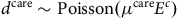 $${d^{{\rm{care}}}}\sim {\rm{Poisson}}\left( {{\mu ^{{\rm{care}}}}{E^c}} \right)$$
where ${\mu ^{{\rm{mort}}}}$
and
${\mu ^{{\rm{mort}}}}$
and ${\mu ^{{\rm{care}}}}$
are the hazards for mortality and long-term care, respectively. In contrast,
${\mu ^{{\rm{care}}}}$
are the hazards for mortality and long-term care, respectively. In contrast, $q$
-type modelling has little theoretical support beyond binomial trials, which don’t permit multiple types of event. The classical actuarial approach is to try to create an artificial single-decrement equivalence by reducing the number of lives:
$q$
-type modelling has little theoretical support beyond binomial trials, which don’t permit multiple types of event. The classical actuarial approach is to try to create an artificial single-decrement equivalence by reducing the number of lives:
 $${d^{{\rm{mort}}}}\sim {\rm{Binomial}}\left( {{q^{{\rm{mort}}}},{n^{{\rm{mort}}}}} \right),{\rm{and}}$$
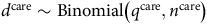 $${d^{{\rm{care}}}}\sim {\rm{Binomial}}\left( {{q^{{\rm{care}}}},{n^{{\rm{care}}}}} \right)$$
where ${q^{{\rm{mort}}}}$
and
${q^{{\rm{mort}}}}$
and ${q^{{\rm{care}}}}$
are the probabilities of mortality and long-term care, respectively.
${q^{{\rm{care}}}}$
are the probabilities of mortality and long-term care, respectively. ${n^{{\rm{mort}}}}$
and
${n^{{\rm{mort}}}}$
and ${n^{{\rm{care}}}}$
are pseudo-life-counts, both less than
${n^{{\rm{care}}}}$
are pseudo-life-counts, both less than $n$
. It is traditional to use an approximation like the following from Benjamin and Pollard (Reference Benjamin and Pollard1986), equation (2.1):
$n$
. It is traditional to use an approximation like the following from Benjamin and Pollard (Reference Benjamin and Pollard1986), equation (2.1):
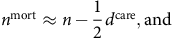 $${n^{{\rm{mort}}}} \approx n - {1 \over 2}{d^{{\rm{care}}}},{\rm{and}}$$
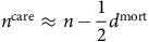 $${n^{{\rm{care}}}} \approx n - {1 \over 2}{d^{{\rm{mort}}}}$$
The lack of rigour with the $q$
-type approach to competing decrements can be seen when we apply it to our example:
$q$
-type approach to competing decrements can be seen when we apply it to our example:
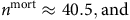 $${n^{{\rm{mort}}}} \approx 40.5,{\rm{and}}$$
 $${n^{{\rm{care}}}} \approx 39.5.$$
But what is 0.5 of a binomial trial? Half a person? The binomial likelihood can still be evaluated and maximized for non-integral values for the number of trials, but the $q$
-type models in Equations (3) and (4) clearly do not correspond to reality.
$q$
-type models in Equations (3) and (4) clearly do not correspond to reality.
7. Data-quality Checks
Continuous-time methods also offer better checks of data quality. We look at how data issues can be revealed by a non-parametric estimate of survival by age, and a semi-parametric estimate of mortality hazard in time.
7.1. Non-Parametric Survival Curve by Age
The estimator from Kaplan and Meier (Reference Kaplan and Meier1958) estimates the survival curve at intervals determined by the time between deaths (the definition from Fleming and Harrington (Reference Fleming and Harrington1991) does something very similar). In the case of many actuarial portfolios, this interval is often as small as one day, making the Kaplan-Meier estimate effectively a continuous-time measure; see Section D.1 in Appendix D. An example is shown in Figure 12(a).
Kaplan-Meier survival curves from age 60 for (a) the Scottish pension scheme in Figure 5 and (b) a UK annuity portfolio. The odd shape of the survival curve for the UK annuitants, and the lack of a male-female differential between ages 60–80, suggests a data-corruption problem like the one described in Case Study A.6 in Appendix A.
Source: Macdonald et al. (Reference Macdonald, Richards and Currie2018), Figure 2.8.
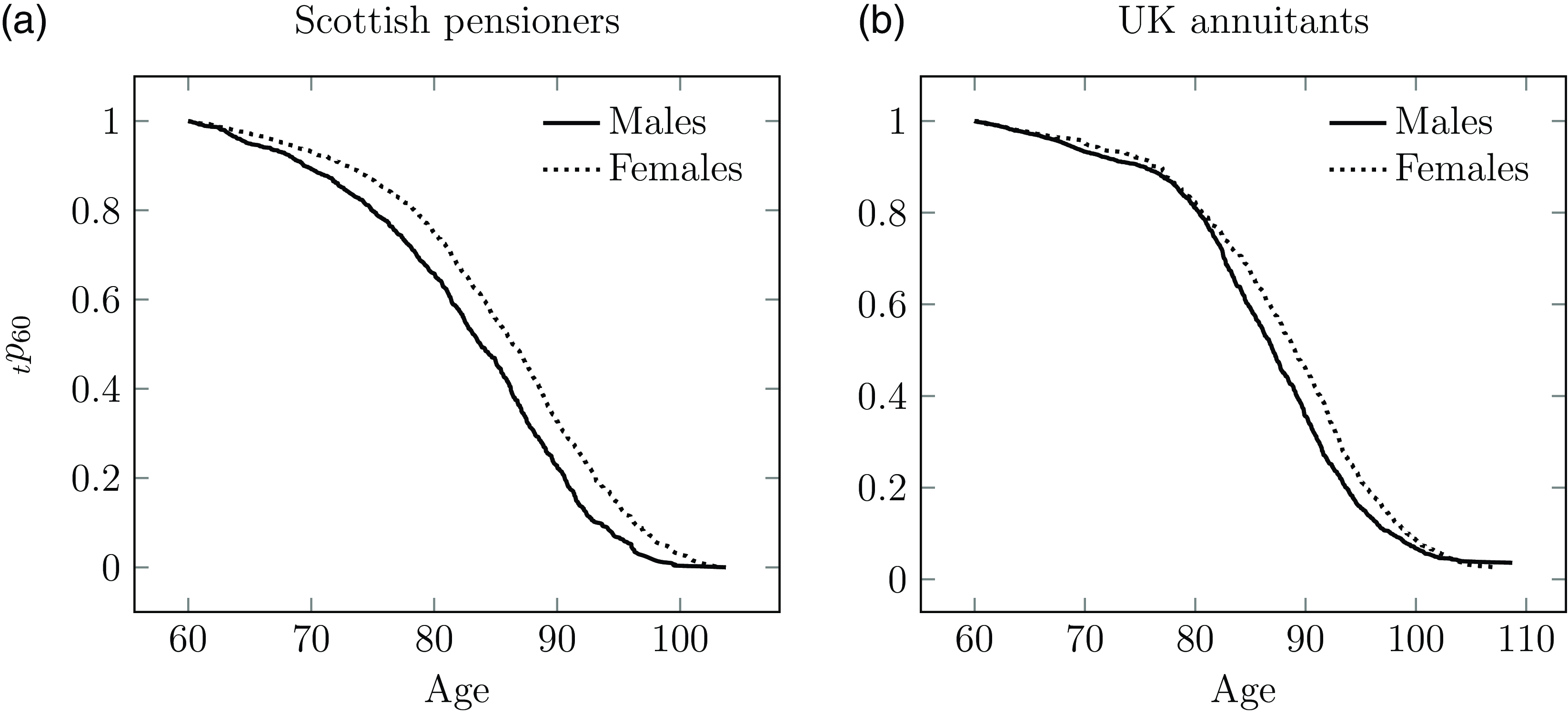
The value of the Kaplan-Meier estimate as a data-quality check is shown in Figure 12(b), where the odd shape and the lack of a male-female differential between ages 60 and 80 suggests a data-quality problem. Case Study A.6 in Appendix A describes a possible cause. Note that this sort of problem is trickier to detect with a traditional comparison of age-grouped mortality against a standard table. The visual nature of the Kaplan-Meier estimate is also a major advantage when communicating with non-specialists. See also Case Studies A.2 and A.3 in Appendix A.
7.2. Semi-Parametric Hazard Over Time
Richards (Reference Richards2022b) proposed a semi-parametric estimate for the mortality hazard of a portfolio over time, and the details of its calculation are given in Section D.5 in Appendix D. Figure 13(a) shows the seasonal variation in a Scottish pension scheme, with particularly high mortality in the winter of 2002–2003. In contrast, the much larger Canadian pension plan in Figure 13(b) shows seasonal variation only from 2016 onwards, raising questions about the data quality in 2014 and 2015. Closer inspection of the Canadian mortality reveals that deaths are recorded continuously throughout the year, but that the first of each month has disproportionately more deaths than other times during the same month. This suggests an inconsistent approach to the recording of the date of death; see also Case Study A.15 in Appendix A. Detailed inspection showed that this data anomaly is present throughout the entire period shown in Figure 13(b), but it is more dominant in 2014 and 2015 and thus more visually apparent.
Estimated aggregate hazard in time for (a) the Scottish pension scheme in Figure 5 and (b) a Canadian pension plan with more lives and deaths. The Canadian pension plan is missing the expected seasonal pattern in 2014 and 2015, raising questions over the accuracy of the experience data during that period.
Source: Adapted from Richards (Reference Richards2022b), Figure A.2.
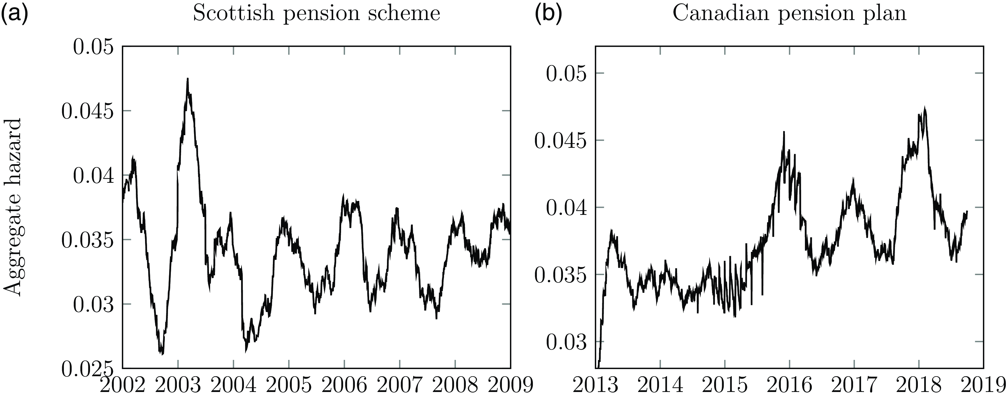
The mortality spike in the winter of 2002–2003 in Figure 13(a) raises a question: why would one exclude Covid mortality spikes, when such seasonal spikes have typically been left in?
8. Management Information
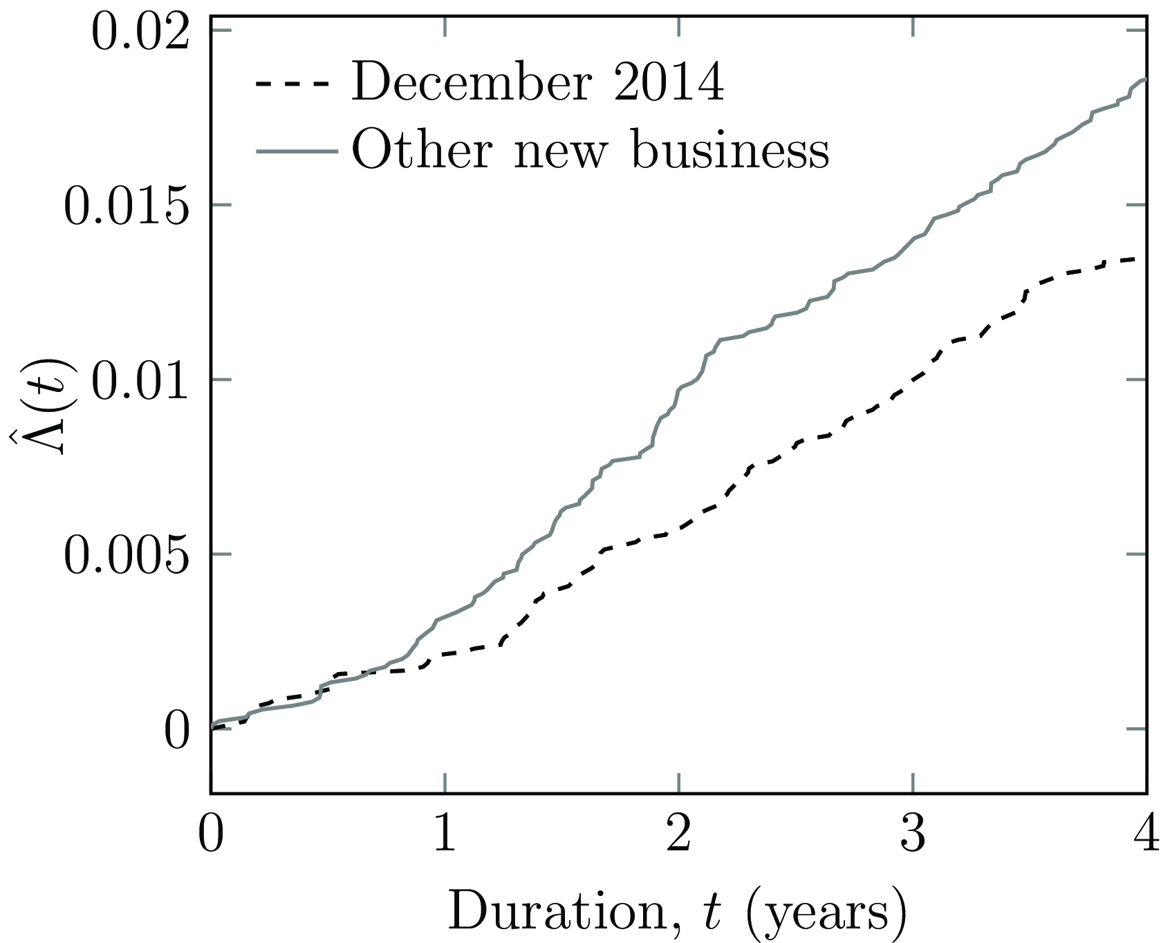
A major advantage of continuous-time methods is their ability to give timely and ongoing answers to management questions. For example, consider the surge in new business shown in December 2014 in Figure 4(a). The average age at commencement of the 9,570 new annuitants in December 2014 is 60.75 years. This is close to the average age at commencement of 61.34 years for the 9,033 new annuitants in the six months before and after December 2014. Although the commencement ages are very close, a natural management question is whether the mortality of the December 2014 annuitants is different from other recent new business? Figure 14 shows that this is indeed the case, with the December 2014 annuitants experiencing lighter mortality than their contemporaries. The statistic used here is the Nelson-Aalen estimate of Equation (D2) (see Section D.2), which can be updated continuously without waiting for a complete year of exposure as with a $q$
-type analysis; Figure 14 could be updated weekly, for example. This is a critical advantage when entering a new market; see Case Study A.8 in Appendix A.
$q$
-type analysis; Figure 14 could be updated weekly, for example. This is a critical advantage when entering a new market; see Case Study A.8 in Appendix A.
Nelson-Aalen estimate, $\hat \Lambda \left( t \right)$
, of cumulative mortality rate for new business written (i) in December 2014, and (ii) in the six months on each side of December 2014.
$\hat \Lambda \left( t \right)$
, of cumulative mortality rate for new business written (i) in December 2014, and (ii) in the six months on each side of December 2014.
Source: Own calculations using new annuities written by the French insurer in Figure 4.
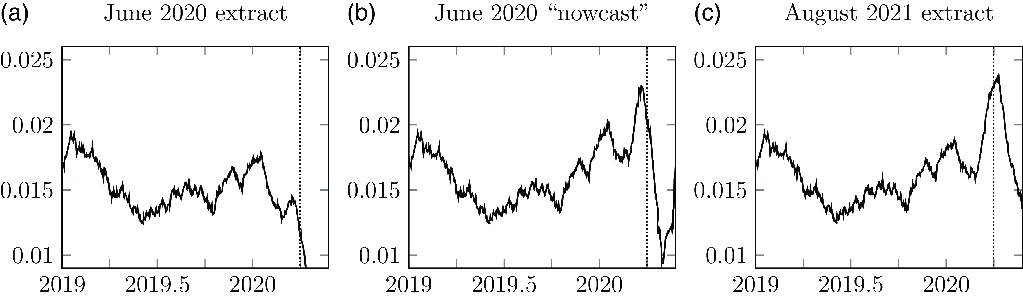
Of course, the phenomenon of OBNR deaths discussed in Section 4.3 is a challenge for any methods using current data. However, as shown in Figure 9, continuous-time semi-parametric methods can also be used to estimate the timing and incidence of OBNR. If need be, graphs such as Figure 14 can be adjusted to allow for OBNR. This is analogous to the econometric techniques of “nowcasting” (Bańbura et al., Reference Bańbura, Giannone, Modugno, Reichlin, Elliott and Timmermann2013), where the most recently available information is used to estimate the current value of a statistic that won’t be fully known until sufficient time has elapsed. This is illustrated in Figure 15(a), where the June 2020 data extract shows no sign of the pandemic mortality expected in April & May 2020. An allowance for OBNR allowed a “nowcast” of mortality, as shown in Figure 15(b). A later data extract used in Figure 15(c) shows that the OBNR-adjusted “nowcast” in panel (b) was accurate enough for business planning at the time it was made. ${\hat \mu _{2019}}\left( t \right)$
for French annuity portfolio with smoothing parameter
${\hat \mu _{2019}}\left( t \right)$
for French annuity portfolio with smoothing parameter $c = 0.1$
: (a) calculated using June 2020 extract; (b) nowcast using Gaussian OBNR function estimated from June 2020 extract; (c) calculated using August 2021 extract. The vertical dotted line in each panel is at 1st April 2020.
$c = 0.1$
: (a) calculated using June 2020 extract; (b) nowcast using Gaussian OBNR function estimated from June 2020 extract; (c) calculated using August 2021 extract. The vertical dotted line in each panel is at 1st April 2020.
9. Discussion
The problems of single-decrement $q$
-type models in Section 3 can be partially solved by discarding some records and editing others. However, throwing away data is a luxury that not every analyst can afford; see Case Studies A.5 and A.7 in Appendix A. Furthermore, modifying the data to suit the needs of the model is surely the wrong direction of causality – a model should be picked that suits the data, not the other way around. As shown in Section 3, continuous-time methods are a better match to the reality of business processes on most administration systems.
$q$
-type models in Section 3 can be partially solved by discarding some records and editing others. However, throwing away data is a luxury that not every analyst can afford; see Case Studies A.5 and A.7 in Appendix A. Furthermore, modifying the data to suit the needs of the model is surely the wrong direction of causality – a model should be picked that suits the data, not the other way around. As shown in Section 3, continuous-time methods are a better match to the reality of business processes on most administration systems.
The challenges of $q$
-type models in Section 4 can be addressed by reducing the fixed observation period to a quarter-year, or even a month. However, if the answer is to increase granularity, why not use the full detail afforded by the data, namely daily intervals? Administration systems hold lots of dates, which are a natural fit for continuous-time methods.
$q$
-type models in Section 4 can be addressed by reducing the fixed observation period to a quarter-year, or even a month. However, if the answer is to increase granularity, why not use the full detail afforded by the data, namely daily intervals? Administration systems hold lots of dates, which are a natural fit for continuous-time methods.
Alternatively, $q$
-type models can be fitted using bespoke likelihoods for fractional years of exposure, as covered in Appendix B. However, if the analyst is able to do this, then a
$q$
-type models can be fitted using bespoke likelihoods for fractional years of exposure, as covered in Appendix B. However, if the analyst is able to do this, then a $\mu $
-type model will be more flexible and require less data preparation.
$\mu $
-type model will be more flexible and require less data preparation.
Individual records and exact dates allow the use of insightful non- and semi-parametric methods, as shown in Section 7. The Kaplan-Meier curve is a particularly useful tool for detecting subtle data-quality problems. And if one is anyway extracting individual records for data-checking, it makes sense to continue by modelling individual lifetimes if one can. The continuous-time representation attempts to describe these left-truncated, right-censored lifetimes as they really are (and presumably good business data processes share that aim to some extent). In contrast, the discrete-time representation for $q$
-type models works the other way, and attempts to force nature (and the data) to look like a life table.
$q$
-type models works the other way, and attempts to force nature (and the data) to look like a life table.
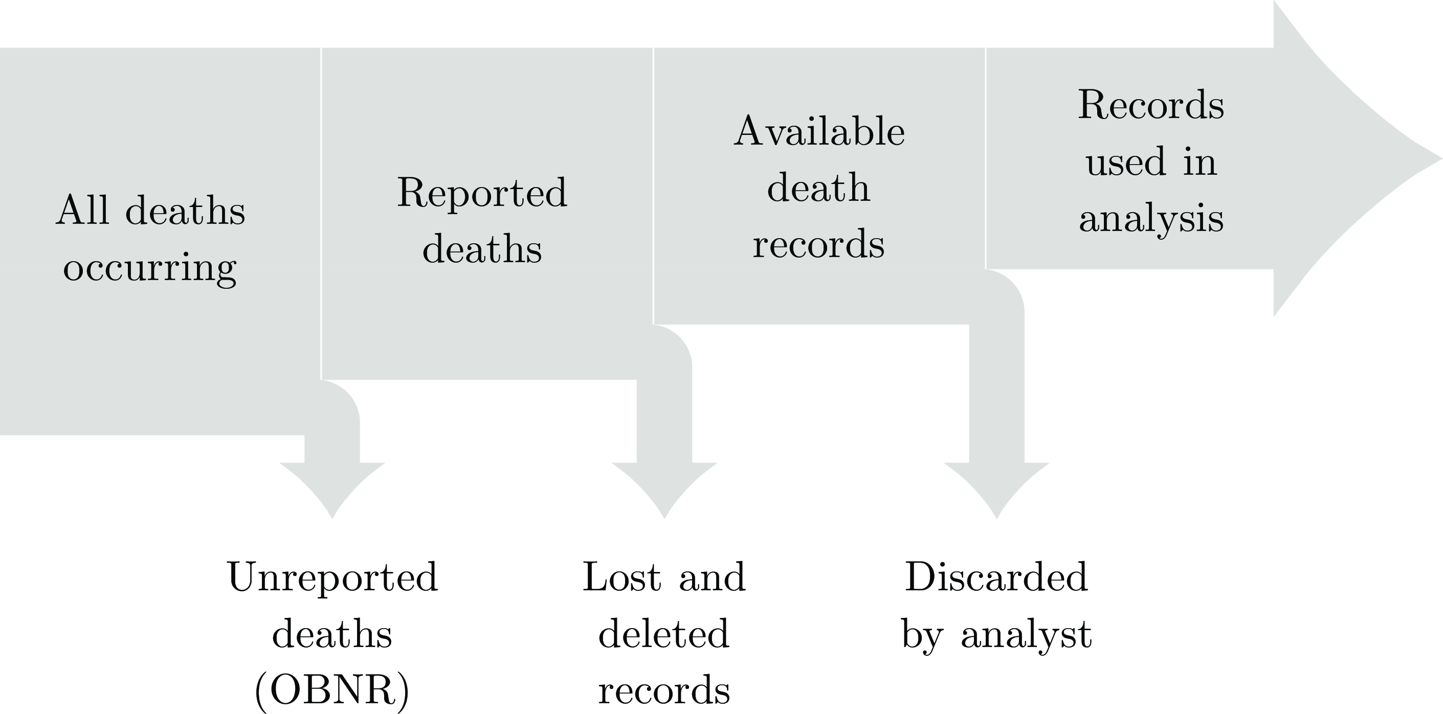
Figure 16 depicts the main categories of data loss between reality on the left and what the analyst has to work with on the right. There is not much that can be done about the middle sources of data loss: if records have been deleted or destroyed, they are unavailable to any type of model. However, $\mu $
-type models can deal with OBNR deaths better than
$\mu $
-type models can deal with OBNR deaths better than $q$
-type models, and less data is discarded with continuous-time methods than discrete-time ones.
$q$
-type models, and less data is discarded with continuous-time methods than discrete-time ones.
Cumulative loss of mortality data in a portfolio.
10. Conclusions
Methods operating in continuous time, or in daily intervals, offer substantial advantages for actuaries. Chief among these are the ability to reflect the reality of everyday business processes, and the ability to handle rapid changes in risk level. In contrast, $q$
-type models, especially those operating over a one-year interval, make assumptions about the data that are hard to justify, and often require data to be discarded if using standard GLMs. In addition, annual
$q$
-type models, especially those operating over a one-year interval, make assumptions about the data that are hard to justify, and often require data to be discarded if using standard GLMs. In addition, annual $q$
-type models are unable to reflect rapid intra-year movements in risk.
$q$
-type models are unable to reflect rapid intra-year movements in risk.
Continuous-time methods are also the more practical solution to certain modelling problems. Examples include risks varying in more than one time dimension and modelling risks with competing decrements. In contrast, annual $q$
-type models within a GLM framework are not capable of simultaneously modelling time- and duration-varying risk. For competing risks,
$q$
-type models within a GLM framework are not capable of simultaneously modelling time- and duration-varying risk. For competing risks, $q$
-type models force the pretence that the number of lives is smaller than it really is.
$q$
-type models force the pretence that the number of lives is smaller than it really is.
Continuous-time methods also offer useful data-quality checks. The visual nature of non- and semi-parametric methods make them particularly useful for communication with non-specialists.
There are occasional circumstances when daily information is unavailable, or even deliberately withheld, but actuaries should strive wherever possible to collect full dates and use continuous-time methods of analysis.
Acknowledgements
The authors thank Gavin Ritchie, Stefan Ramonat, Patrick Kelliher, Kai Kaufhold and Ross Ainslie for comments on earlier drafts. Any errors in the paper are the sole responsibility of the authors. The authors also thank the owner of the home-reversion portfolio in Case Study A.32, who wishes to remain anonymous. This document was typeset in LaTeX. Graphs were created with tikz (Tantau, Reference Tantau2024) and pgfplots (Feuersänger, Reference Feuersänger2015).
Appendices
A. Case Studies
The following are case studies are based on actual experience. In most case studies, continuous-time methods provided important benefits over $q$
-type models.
$q$
-type models.
Case Study A.1
The Pension Benefit Guaranty Corporation (PBGC) in the United States charges a flat annual fee of $37 per participant in a multi-employer pension plan in 2024, rising to $52 in 2031 (PBG, 2024, Table M-16). For single-employer plans the flat part of the annual fee is $101 per participant in 2024, with an additional variable fee of up to $686 per participant for unfunded vested liabilities (PBG, 2024, Table S-39). To minimize payments to the PBGC, a pension plan therefore buys annuities to close out the liabilities for the individuals with the smallest pensions. The pensions that are bought out are treated like commutations, with the observation end date being the date of annuity purchase.
A continuous-time model can include the bought-out annuities, as they will be like Case C in Figure 1. Note that the PBGC fee is per participant, so there is a financial benefit from identifying multiple records relating to the same person among retained cases; see the discussion of deduplication in Macdonald et al. (Reference Macdonald, Richards and Currie2018), Section 2.5.
Case Study A.2
A consulting actuary is asked by a reinsurer to set a pricing basis for a longevity swap. However, the Kaplan-Meier curves for males and females exhibit a pattern like that of Figure 12(b), suggesting that the data are corrupted. The consultant informs the reinsurer, which asks the cedant for better-quality data. The cedant refuses, and the consultant recommends that the reinsurer walks away from the transaction, which it does.
Case Study A.3
A consulting actuary is asked by the sponsoring employer of a pension scheme to validate the mortality basis used for funding calculations. The consulting actuary calculates the Kaplan-Meier curves for males and females and, like Case Study A.2, finds a pattern like that of Figure 12(b), suggesting that the data are corrupted. The third-party pension-scheme administrator is ordered to implement a data clean-up programme, which produces better data and thus allows a reliable basis to be derived.
Case Study A.4
The insurer of the annuities in Figure 3 needs to set a mortality basis for the year-end valuation in 2015. A simple multi-year comparison against a standard table is inappropriate, as Figure 3(b) shows that the transferred annuities are not a random sample of the overall portfolio. A $q$
-type analysis is complicated by the exit from observation of 60,000 annuities during 2013. A better solution is a
$q$
-type analysis is complicated by the exit from observation of 60,000 annuities during 2013. A better solution is a $\mu $
-type analysis, using the date of the last annuity payment on the system as a proxy for the date of right-censoring. This allows both transferred and remaining annuities to receive the same treatment as Cases A and B in Figure 1. Such a solution works best for annuities paid relatively frequently, e.g. monthly.
$\mu $
-type analysis, using the date of the last annuity payment on the system as a proxy for the date of right-censoring. This allows both transferred and remaining annuities to receive the same treatment as Cases A and B in Figure 1. Such a solution works best for annuities paid relatively frequently, e.g. monthly.
Case Study A.5
An actuary is tasked with setting a mortality basis for a large annuity portfolio. Eighteen months before the actuary’s appointment, annuities in payment were migrated to a new administration platform and records of prior deaths were lost. The actuary only has one-and-a-half years of experience data. Annuities set up before the migration are therefore like Cases D and E in Figure 1, whereas newer annuities set up post-migration are like Cases A and B.
The portfolio has scale in terms of the number of annuities, but it has no depth in terms of historic data. Using an annual $q$
-type GLM makes this depth problem even worse: the requirement for a complete year of potential exposure means discarding a third of what little historical data is available. The most recent half-year of experience would be discarded in order not to have mortality levels under-stated due to delays in reporting of deaths. Much of the new business written would therefore also be excluded from
$q$
-type GLM makes this depth problem even worse: the requirement for a complete year of potential exposure means discarding a third of what little historical data is available. The most recent half-year of experience would be discarded in order not to have mortality levels under-stated due to delays in reporting of deaths. Much of the new business written would therefore also be excluded from $q$
-type analysis, robbing the actuary of information on possible selection effects.
$q$
-type analysis, robbing the actuary of information on possible selection effects.
In contrast, a continuous-time solution is to model ${\mu _x}$
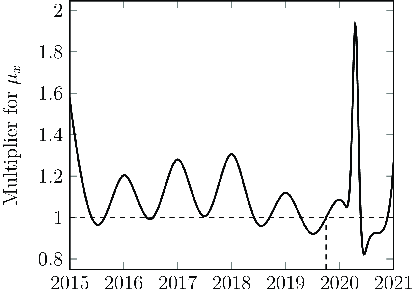
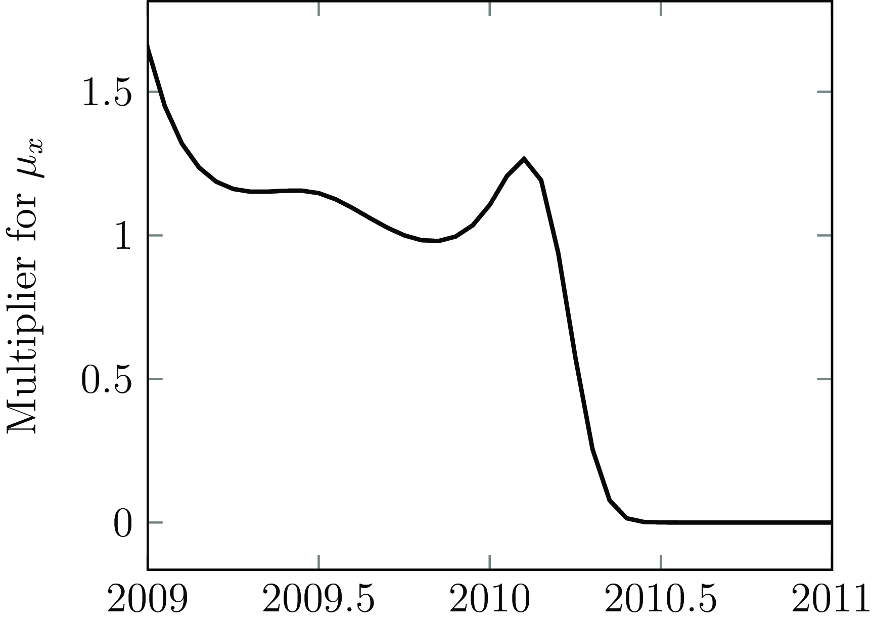
and use all eighteen months of data, including the new business. Delays in reporting of recent deaths could be handled either by using a parametric OBNR term (Richards, Reference Richards2022b) or using the approach of Richards (Reference Richards2022c), as illustrated in Figure A1. In the latter case, the level of mortality to use for a long-term purpose like valuation would have to be decided by judgement, say by picking the modelled (and thus smoothed) mortality level mid-way between a winter peak and a summer trough.
${\mu _x}$
and use all eighteen months of data, including the new business. Delays in reporting of recent deaths could be handled either by using a parametric OBNR term (Richards, Reference Richards2022b) or using the approach of Richards (Reference Richards2022c), as illustrated in Figure A1. In the latter case, the level of mortality to use for a long-term purpose like valuation would have to be decided by judgement, say by picking the modelled (and thus smoothed) mortality level mid-way between a winter peak and a summer trough.
Mortality multiplier over time for French annuity portfolio, with multipliers standardized at 1 for October 2009. The data extract was taken in mid-2010, and the impact of reporting delays (OBNR) is very pronounced.
Source: Own calculations using flexible B-spline basis for mortality levels described in Richards (Reference Richards2022c).
Case Study A.6
A pricing analyst is looking for risk factors to use for annuitant mortality. One of the data fields available is whether an annuity has an attaching spouse’s benefit, i.e. a contingent annuity that commences on death of the first life. Statistical modelling suggests that the presence or absence of a spouse’s benefit is highly significant, and has a mortality effect on a par with the sex of the annuitant. The direction of the effect is plausible, with single-life annuitants exhibiting higher mortality (Ben-Shlomo et al., Reference Ben-Shlomo, Smith, Shipley and Marmot1993).
However, the analyst is aware of the potential for record corruption from Case Study A.2. Specifically, if the main annuitant dies and the spouse is then discovered to have pre-deceased them, the record of the contingent benefit might be removed during death processing. This would make the annuity look like a single-life annuity from outset, and thus distort the apparent mortality differential. The analyst emails the IT department with his concerns and is told that they are unfounded. Sceptical, he makes a further telephone enquiry and is again assured that the feared corruption is not present.
Believing that he may have found an important new risk factor for pricing, the analyst writes a note to the chief actuary. The analyst then remembers that these quality assurances come from the same IT department that lost all the mortality data in Case Study A.5. The analyst performs a third investigation, and discovers that his original suspicions were correct. The excess mortality for single-life annuitants has been grossly exaggerated by the deletion of pre-deceased spouse records.
Case Study A.7
An insurer with a large annuity portfolio has an administration system that automatically deletes records of annuitants who died more than two years in the past. Annuities are set up like Cases A and B in Figure 1, but after two years a Case A annuity becomes like Case D, while Case B annuities simply disappear from the administration system entirely. An urgent request is made to stop this rolling deletion of valuable data.
Similar to Case Study A.5, an annual $q$
-type GLM only permits the use of a single year of data – the most recent six months are ignored due to late-reported deaths, leaving 1.5 years of data, but a further half-year of unaffected data also has to be discarded to meet the requirement of only using complete years.
$q$
-type GLM only permits the use of a single year of data – the most recent six months are ignored due to late-reported deaths, leaving 1.5 years of data, but a further half-year of unaffected data also has to be discarded to meet the requirement of only using complete years.
As in Case Study A.5, a continuous-time solution is to model ${\mu _x}$
and use all two years of data. Delays in reporting of recent deaths could be handled either by using a parametric OBNR term (Richards, Reference Richards2022b) or using the approach of Richards (Reference Richards2022c), as illustrated in Figures 6 and A1. As in Case Study A.5, the level of mortality would be chosen by judgement, such as a modelled value from spring or autumn.
${\mu _x}$
and use all two years of data. Delays in reporting of recent deaths could be handled either by using a parametric OBNR term (Richards, Reference Richards2022b) or using the approach of Richards (Reference Richards2022c), as illustrated in Figures 6 and A1. As in Case Study A.5, the level of mortality would be chosen by judgement, such as a modelled value from spring or autumn.
Case Study A.8
A UK insurer has historically written annuities based solely on the experience of its own maturing money-purchase pension policies. The insurer decides to enter the open market for non-underwritten annuities. However, there is a parallel open market for underwritten annuities, where better terms are offered to lives with demonstrable health conditions (Ainslie, Reference Ainslie2000). The insurer is concerned that the existence of the underwritten market creates selection effects in the new open-market standard annuities that it is writing. The experience data of annuitants from its own maturing pension policies are not believed to have such selection effects, so the new mortality pricing basis contains some guesswork (Richards and Robinson, Reference Richards and Robinson2005).
At the end of the first year of the new strategy the insurer wants to urgently (i) validate its pricing assumptions with respect to selection and (ii) set a valuation mortality basis for the new open-market annuities. This cannot be done particularly cleanly using ${q_x}$
models, as a full year of exposure has not yet been achieved for the new business. In contrast, a continuous-time analysis based on
${q_x}$
models, as a full year of exposure has not yet been achieved for the new business. In contrast, a continuous-time analysis based on ${\mu _x}$
can easily handle the fractional exposures of the annuities written during the year, with no special modifications required; see Richards (Reference Richards2020), Section 6 for an example.
${\mu _x}$
can easily handle the fractional exposures of the annuities written during the year, with no special modifications required; see Richards (Reference Richards2020), Section 6 for an example.
See also the related discussion around Figure 14.
Case Study A.9
A medium-sized UK pension scheme provides data for analysis. Inspection of the data suggests that temporary and commuted pensions have been erroneously marked as deaths; see Figure A2, where almost all 20 year-olds are allegedly die. This indicates that the data have not been properly processed. In particular, the mortality of recipients of small pensions may be considerably over-stated due to commuted cases being misclassified as deaths.
Case Study A.10
A Canadian pension plan will not provide full dates of death, as Canadian privacy laws apply to those who have died in the past twenty years (PIP, 2018). Instead, only the year and month of death are provided.
Since we only know the month in which death occurs, this is interval censoring (Macdonald, Reference Macdonald1996, Section 2.3). A continuous-time model can be built assuming that deaths take place on the 15 $^{{\rm{th}}}$
of the month. The distortion will be small, with the actual date of death being on average only a week away from this assumption (and with average deviations being close to zero). Note, however, that the tracking statistic of Richards (Reference Richards2022b) will be affected by this loss of information, and the Kaplan-Meier survival curve will have a more ridged appearance than would be the case with exact dates of death.
$^{{\rm{th}}}$
of the month. The distortion will be small, with the actual date of death being on average only a week away from this assumption (and with average deviations being close to zero). Note, however, that the tracking statistic of Richards (Reference Richards2022b) will be affected by this loss of information, and the Kaplan-Meier survival curve will have a more ridged appearance than would be the case with exact dates of death.
Case Study A.11
An insurer is thinly capitalized with a small solvency margin. In the hope of lowering its capital requirements, the insurer asks for reinsurance quotations for its large annuity portfolio. However, even the cheapest reinsurance quotation has a mortality basis that is stronger than the insurer’s existing reserving basis. This would require the insurer to pay an up-front premium, which it cannot afford.
While the insurer can of course decline to reinsure, it cannot now leave its annuitant mortality basis unchanged. It has just discovered the market price for its annuitant mortality, and must now strengthen its mortality basis.
Case Study A.12
An insurer with a large annuity portfolio needs to plan staffing levels. In particular, the work processing death notifications is often upsetting and stressful, and limits are in place for the amount of time an individual member of staff can be assigned to this task. The insurer uses a mortality model with a season term (see Section 4.4) to make short-term forecasts of likely deaths, thus informing staffing requirements and rotas.
Case Study A.13
An insurer has assumed the annuity liabilities of another insurer. In the UK this is a court-sanctioned process known as a Part VII transfer (FSM, 2000, PartVII). The IT department sets up the transferred annuities on the administration system with the original commencement date. This makes it difficult to separately identify the transferred annuities, which is problematic because there are periods of survival between commencement and transfer without corresponding deaths.
A continuous-time solution is to use the date of the first annuity payment on the new system as a proxy for the transfer-in date. This allows the new liabilities to be treated like Cases D and E in Figure 1. As in Case Study A.4, such a solution works best for annuities paid relatively frequently, e.g. monthly.
Case Study A.14
In contrast to Case Study A.13, a system migration takes place where the commencement date on the new system is the date of migration, not the original date of retirement (which is then lost).
The migrated cases look like Cases A and B in Figure 1, but in reality they are like Cases D and E. The exposure period can be calculated, but no modelling of duration or selection effects can take place due to not having the actual retirement date.
Case Study A.15
An insurer runs a programme to identify unreported annuitant deaths. Instead of using the actual date of death, the insurer processes the discovered cases en masse using the date of processing, resulting in a large spike in deaths recorded for that particular date.
Here the survival times are unreliable for the mass-processed cases. Superficially, it might seem preferable to use a model that specifically discards precise survival times, i.e. a $q$
-type analysis. However, this is only likely to be true if such exercises are carried out sufficiently regularly that the inaccuracy of the date of death is modest. There is a strong financial incentive to run regular existence-verification exercises, say quarterly, as each identified case will release reserves. For this reason it is particularly beneficial to run such exercises prior to the year-end statutory valuation.
$q$
-type analysis. However, this is only likely to be true if such exercises are carried out sufficiently regularly that the inaccuracy of the date of death is modest. There is a strong financial incentive to run regular existence-verification exercises, say quarterly, as each identified case will release reserves. For this reason it is particularly beneficial to run such exercises prior to the year-end statutory valuation.
Case Study A.16
A UK insurer has written a lot of bulk annuity business and thus has significant liabilities for both pensions in payment and deferred pensions. The actuary is tasked with setting a basis for both sub-types of business, which are administered on the same computer system.
The occurred-but-not-reported (OBNR) deaths for pensions in payment is a relatively contained problem. While there are reporting delays, they can be measured and allowed for, as described in Section 4.3. Part of the reason for this is that the insurer has a constant feedback mechanism – most UK pension payments are made via automated bank credit (BACS Direct Credit, 2019), and there is a specific rejection code for an attempt to pay money into the account of a decedent (ARUCS2 – Beneficiary Deceased).
However, the situation for deferred pensions is different – with no premiums to collect or payments to make, the reporting of deaths of deferred pensioners is typically sparse with very long delays. It is not uncommon for the insurer to only find out about a past death when it tries to make the first pension payment at retirement age. It is therefore common for the mortality data for deferred liabilities to be unreliable, and for a basis to be derived without reference to experience data.
The situation for deaths of deferred pensions can sometimes be improved by the regular use of third-party services, which provide matches to known deaths of varying degrees of confidence based on name, date of birth and last known address. However, it is important to use such external data thoughtfully, as clumsy application can lead to bad publicity (Tims, Reference Tims2024).
Case Study A.17
The German multi-employer pension scheme in Richards et al. (Reference Richards, Kaufhold and Rosenbusch2013) stores only the year of death. The data collected by the pension scheme have been designed for $q$
-type analysis only. The exact date of death could be obtained from another source, but the third-party administrator demands payment for bespoke work not covered by the service contract. An additional issue is that pensioners dying during the calendar year of retirement are not recorded at all, being neither in the in-force at the start of the year nor in the deaths.
$q$
-type analysis only. The exact date of death could be obtained from another source, but the third-party administrator demands payment for bespoke work not covered by the service contract. An additional issue is that pensioners dying during the calendar year of retirement are not recorded at all, being neither in the in-force at the start of the year nor in the deaths.
If this were an insurer concerned about anti-selection, as in Case Study A.8, then it might be worth paying for the exact dates of death for a continuous-time model. However, for a pension scheme with slowly changing membership, the cost was not felt to be justified. A ${q_x}$
model could be built with the data, or else a
${q_x}$
model could be built with the data, or else a ${\mu _x}$
model assuming that all deaths occur in the middle of the year. Two further consequences of not knowing the date of death are that (i) the tracking statistic of Richards (Reference Richards2022b) cannot be used, and (ii) the Kaplan-Meier survival curves will take a pronounced step shape, as exact ages of death are not known.
${\mu _x}$
model assuming that all deaths occur in the middle of the year. Two further consequences of not knowing the date of death are that (i) the tracking statistic of Richards (Reference Richards2022b) cannot be used, and (ii) the Kaplan-Meier survival curves will take a pronounced step shape, as exact ages of death are not known.
Case Study A.18
An annuity portfolio has been administered continuously since outset on the same computer system without any record deletion, archiving of historic deaths or migration onto or off the system. All annuity records are like Cases A, B and C in Figure 1, and it would be possible to model mortality along these lines if (i) mortality levels were stable, (ii) mortality differentials were stable and (iii) selection effects were stable. However, in practice these things change over time, so most organizations restrict their modelling to the most recent experience, such as the past five years. This means that older annuities are deliberately turned from Cases A and B into Cases D and E, respectively (and very old Cases B and C are excluded entirely). See also Figure 11 for an illustration of the application of such an investigation “window.”
Note that such continuity of experience can also be found with some very large, self-administered pension schemes. The outsourcing of pension-scheme administration is invariably bad news for the mortality experience data, especially changes of administrator.
Case Study A.19
An analyst at a UK insurer is directed to use the annual valuation extracts for analysis. The extracts are policy-orientated and have been validated for year-end statutory balance sheet calculations. However, the valuation extracts contain neither names nor postcodes, so the analyst cannot perform the deduplication necessary for statistical modelling (Macdonald et al., Reference Macdonald, Richards and Currie2018, Section 2.5). The absence of postcodes further means that geodemographic mortality modelling cannot be done either (Macdonald et al., Reference Macdonald, Richards and Currie2018, Section 2.8.1). Finally, the annual “snapshot” nature of the valuation extracts means that policies that commence and terminate during the calendar year are not included, thus hampering the modelling of anti-selection.
The analyst therefore arranges for a direct extract of policy records from the administration system. Also, since mortality models routinely use geodemographic profiles (Madrigal et al., Reference Madrigal, Matthews, Patel, Gaches and Baxter2011), a request is made to add postcodes to future valuation extracts.
Case Study A.20
Many valuation systems are heavily restricted in the mortality risk factors they can cope with. It is common to have the flexibility to upload a new mortality table of ${q_x}$
rates, but this typically limits the calculations to using just age and sex as risk factors. Beyond this, such systems sometimes also allow the application of a multiplier to the
${q_x}$
rates, but this typically limits the calculations to using just age and sex as risk factors. Beyond this, such systems sometimes also allow the application of a multiplier to the ${q_x}$
rates for portfolio-specific customization. This is a problem for modern mortality analysis, which typically uses many more risk factors than just age and sex – see the list in Section 1.
${q_x}$
rates for portfolio-specific customization. This is a problem for modern mortality analysis, which typically uses many more risk factors than just age and sex – see the list in Section 1.
One solution is the equivalent-reserve method popularized by Willets (Reference Willets1999). This involves calculating an annuity factor using the multi-factor mortality model, then finding the percentage of the given mortality table that produces the same value. This is done for various risk factor combinations in Richards et al. (Reference Richards, Kaufhold and Rosenbusch2013), Table 13. However, this approach can be extended to the entire portfolio valuation, thus automatically weighting the mortality risk factors by their impact on the liabilities. The resulting table percentages can then be fed into the valuation system. An important point to note is that financial distortions occur if the resulting table percentage falls far outside the 85–115% range. If this is the case, then it is crucially important to change the reference table so that the percentages are closer to 100%.
Case Study A.21
A US insurer is bidding for a multi-billion dollar buy-out of a large pension plan. The proposed transaction is so large that on its own it will meet the insurer’s new business target for this type of risk. The pricing committee is both keen to win the business, but also worried about the financial impact of possibly getting the mortality basis wrong. A request is made for a statistically rigorous confidence interval around the best estimate of current mortality in the pension plan (the future-improvement assumption is set centrally at the corporate level).
The pricing basis was derived using an individual survival model calibrated to the pension plan’s experience data. This allowed the analysts to use the methodology of Richards (Reference Richards2016) to measure the sensitivity of the liability value to the uncertainty surrounding the parameter estimates. A process of simulating alternative parameter estimates consistent with the covariance matrix produced a thousand alternative valuations of the liabilities. The relevant quantiles of these simulated liabilities were then back-solved using the equivalent-reserve method of Case Study A.20 to produce a confidence interval for the best-estimate mortality pricing assumption.
Case Study A.22
An underfunded UK pension scheme is approached by an advisor suggesting that health questionnaires should be sent to pensioners. Those pensioners qualifying for enhanced annuities due to poor health will then have annuities bought from a specialist insurer. Since the enhanced annuities will typically cost less than the notional reserve held in respect of these pensioners, the advisor argues that this will improve the scheme’s funding position.
However, if pensioners in poorer health are selected out in this way, the remaining lives are by definition the healthier, longer-lived ones. Thus, the scheme’s mortality basis therefore needs to be strengthened for the remaining members after the enhanced-annuity exercise, and there should be no net improvement in the funding position. Furthermore, carrying out this exercise limits future buy-out options for the scheme – some insurers in the UK specifically ask about past ill-health buy-outs, and refuse to quote if such an exercise has been carried out in the preceding five years.
Case Study A.23
An insurer decides that it no longer wants to write annuities for its portfolio of vesting pension policies. It decides instead to operate a small panel of annuity providers and take commission as an introducer. This way the insurer can make money from the annuities without having to carry the liabilities on its balance sheet. The insurer provides the mortality experience of its existing annuity portfolio to prospective annuity writers seeking to join the panel. The mortality experience data contain details of the pension product type and whether a guaranteed annuity rate (GAR) is present.
The panel annuity writers need to calibrate a mortality model specific to the profile of this portfolio, which can be done using survival models; see Richards (Reference Richards2008). It is important to create a differentiated mortality model that, where statistically justified, uses risk factors beyond age, sex, pension size and postcode; see Madrigal et al. (Reference Madrigal, Matthews, Patel, Gaches and Baxter2011) and Richards et al. (Reference Richards, Kaufhold and Rosenbusch2013). Product type, distribution channel and annuity options selected by the policyholder are often signals for higher or lower mortality. The panel annuity writer with the least sophisticated mortality basis will be selected against by winning mainly mispriced business (Ainslie, Reference Ainslie2000).
Case Study A.24
A long-established company has a large pension scheme. The company’s market value has steadily shrunk over the years, while the pension scheme has become rather large. The company wants the pension scheme to buy backing annuities to reduce the volatility in its published financial statements. The nature of the company’s business has changed radically over time, and the workforce and pensioners have changed along with it. The older pensioners are mainly drawn from a formerly blue-collar workforce with occupational exposure to dust and chemicals. In contrast, recent retirees are from a more white-collar workforce running a more services-orientated business.
Pension size is a less-reliable proxy for socio-economic differentials here. Former blue-collar workers tended to have longer periods of service with lower salaries. However, their pension amounts overlap substantially with former higher-salaried white-collar staff, who also had shorter periods of service. A crude comparison against a standard table would not pick up the shift in the nature of the socio-economic profile. This is particularly important here because the older, blue-collar pensioners dominate the death counts, while the younger, white-collar pensioners dominate the liabilities. The preferred solution is to fit a scheme-specific survival model, using the postcode-driven geodemographic profile as a means of identifying the socio-economic differentials; see Richards (Reference Richards2008), Madrigal et al. (Reference Madrigal, Matthews, Patel, Gaches and Baxter2011) and Macdonald et al. (Reference Macdonald, Richards and Currie2018), pages 32–36 for details.
Case Study A.25
A UK insurer wants to reinsure a large block of annuity business exceeding
 $${\unicode{x00A3}}$$
10 billion in reserves. To reduce exposure to a single counterparty, and to open the bidding to smaller and medium-sized reinsurers, the portfolio is split into four different blocks to be bid on separately. The blocks have not been selected randomly, but according to internal criteria of the insurer. The insurer provides the mortality experience of the entire annuity portfolio to prospective bidders.
$${\unicode{x00A3}}$$
10 billion in reserves. To reduce exposure to a single counterparty, and to open the bidding to smaller and medium-sized reinsurers, the portfolio is split into four different blocks to be bid on separately. The blocks have not been selected randomly, but according to internal criteria of the insurer. The insurer provides the mortality experience of the entire annuity portfolio to prospective bidders.
Even if they are only planning on bidding for one or two blocks, bidders will use the entire data set to calibrate a mortality model for pricing. It is important that all relevant risk factors are built into the model, since bidders using simplistic pricing are at risk of winning only the blocks they misprice (Ainslie, Reference Ainslie2000).
Case Study A.26
A large UK pension scheme wants to buy annuities to back the pensions in payment. There is an executive sub-scheme containing former executives, senior managers and the surviving spouses of both. However, the executive sub-scheme is too small for a stand-alone analysis, especially a crude comparison against a standard table. Instead, a mortality model is calibrated by the bidding insurer using age, sex, pension size, geodemographic profile and a binary flag denoting membership of the executive sub-scheme. Unsurprisingly, members of the executive sub-scheme have lower mortality than non-members, even after allowing for risk factors like pension size and geodemographic type. This turns out to be significant for pricing the buy-out, as the executive sub-scheme has a lower average age and thus accounts for a larger share of reserves than is implied by their share of annual pensions in payment.
Case Study A.27
A UK pension scheme has far heavier levels of mortality than predicted by a standard commercial model allowing for age, sex, pension size and geodemographic profile. Much of the workforce in question had past occupational exposure to asbestos, so there are grounds to believe that this is a real result. However, the office-based members of the workforce did not have this exposure. The question is whether the experience data is credible enough to justify a weaker mortality basis than the standard commercial model? And, if so, what is statistically justifiable?
A bespoke mortality basis is derived for the pension scheme using survival models; see Richards et al. (Reference Richards, Kaufhold and Rosenbusch2013) and Madrigal et al. (Reference Madrigal, Matthews, Patel, Gaches and Baxter2011) for examples of scheme-specific risk factors that can be used.
Case Study A.28
A UK insurer wishes to improve its mortality model by using postcodes and geodemographic profiles. However, upon extracting the mortality experience data it finds that almost all deaths have the same postcode, namely that of the insurer’s head office. It transpires that servicing staff change the address of deceased annuitants to avoid accidentally sending post to the dead. From a strict data perspective this is a misuse of the address field, but the business requirement of not further upsetting surviving spouses takes precedence.
It is impossible to calibrate a geodemographic mortality model when only survivors have a residential postcode. The insurer needs to extract the history of address changes for the annuitants, and select the residential postcode for geodemographic profiling. However, it is also possible for an address to be changed to that of a solicitor for an annuitant entering care. Fortunately, good geodemographic profilers in the UK typically distinguish between residential and non-residential postcodes. If a history of addresses is available, the most recent residential profile should be used for modelling.
Case Study A.29
A UK insurer wishes to improve its mortality model by using postcodes and geodemographic profiles. Analysis reveals that UK-resident annuitants without a geodemographic profile have high mortality. Further investigation reveals that postcodes are recorded for these annuitants, but that these postcodes are not listed in the geodemographic profiler database. The geodemographic profiler is used for marketing purposes, and only contains currently valid UK postcodes, of which there are around 1.7 million. There are a further half-million retired postcodes that have been used by the Post Office in years past, but which are no longer in use. However, dead annuitants are more likely to have a retired postcode, and so a bias arises.
The servicing department is unwilling to incur the expense and disruption of updating address details for deceased annuitants. The solution is to get the provider of the geodemographic profiler to back-fill their database with historic postcodes and provide the relevant geodemographic profiles for them. This reduces the bias by assigning geodemographic codes to dead annuitants with out-of-date postcodes.
Case Study A.30
A critical-illness (CI) portfolio has a total of 267 CI claims from almost 130,000 life-years of exposure. A reinsurer wants to assess the extra risk – if any – posed by smokers. However, there are two apparent problems. First, the smokers account for just 56 of the claims and 20,000 life-years of exposure. Second, lapses are vastly more common than CI claims.
The presence of a dominant competing decrement makes a $q$
-type model a poor choice for modelling mortality; see Section 6. The actuary therefore treats lapses as censored observations and fits a
$q$
-type model a poor choice for modelling mortality; see Section 6. The actuary therefore treats lapses as censored observations and fits a $\mu $
-type model for age, sex and smoker status, among other covariates. Despite the small number of smoker CI claims, the model shows conclusively that smokers have a 57% higher CI claim rate than non-smokers, with a standard error of 15%. This gives a p-value of 0.02% for the effect of smoking, i.e. the result is highly significant even for an apparently small number of claims.
$\mu $
-type model for age, sex and smoker status, among other covariates. Despite the small number of smoker CI claims, the model shows conclusively that smokers have a 57% higher CI claim rate than non-smokers, with a standard error of 15%. This gives a p-value of 0.02% for the effect of smoking, i.e. the result is highly significant even for an apparently small number of claims.
Case Study A.31
An investor owns a large portfolio of home-reversion plans. These are residential properties that have been purchased while granting the former owners lifetime tenancy. These are not equity-release mortgages – the investor has purchased the actual properties. Nor are these usufruct arrangements – only the tenants named on the lease can live in the property, and they cannot rent it out to other tenants.
The investor makes money from paying the former owners less than the market value of the property in exchange for the right to live there rent-free. The investor can only take unencumbered possession of the property when the last-named tenant leaves. There are two main decrements of interest to the investor: mortality and inception rates for long-term care (LTC). In the supplied experience data deaths occur nearly four times more frequently than LTC events. However, there is also a number of cases where the tenants bought back their property.
The presence of two competing risks and another decrement makes a $q$
-type model a poor choice; see Section 6. The actuary therefore fits two
$q$
-type model a poor choice; see Section 6. The actuary therefore fits two $\mu $
-type models, one each for mortality and LTC inception. For the mortality model, both LTC and buyback events are treated as censored observations. For the LTC model, both deaths and buybacks are treated as censored observations.
$\mu $
-type models, one each for mortality and LTC inception. For the mortality model, both LTC and buyback events are treated as censored observations. For the LTC model, both deaths and buybacks are treated as censored observations.
Case Study A.32
An actuary is asked to analyse a second, smaller portfolio of UK home-reversion plans (see Case Study A.31 for background details on this type of business). In addition to the expected decrements of mortality and entry into long-term care, the actuary finds some additional decrements, such as voluntary surrender of the lease and divorce of married tenants. Voluntary surrender of the lease was deemed to be a precursor stage of long-term care, e.g. when an elderly tenant moves in with one of their adult children. Divorces are trickier – they are obviously neither mortality nor care-related, but divorce leads to a named tenant being taken off the lease, thus bringing forward the repossession of the property in the same manner as death or entry into long-term care.
The presence of multiple competing risks makes a $q$
-type model a poor choice; see Section 6. The actuary includes voluntary surrenders as events in the modelling of the care decrement. Divorces are handled as censoring events for the lives taken off tenancy agreements, despite their financial impact being similar to mortality and care events.
$q$
-type model a poor choice; see Section 6. The actuary includes voluntary surrenders as events in the modelling of the care decrement. Divorces are handled as censoring events for the lives taken off tenancy agreements, despite their financial impact being similar to mortality and care events.
A plot of the mortality-only survival curves after allowing for competing risks is shown in Figure A3. This exhibits a gap of eight years in the median survival age of males and females, which is far larger than the equivalent gap in standard mortality tables. The gap in Figure A3 is, however, consistent with the experience data of Case Study A.31 (not shown), suggesting that portfolio-specific analysis is essential for this class of business.
Lives and “deaths” at young ages for medium-sized UK pension scheme. Temporary pensions to children cease once they leave full-time education, but such cessations have been erroneously labelled as deaths in the data extract.
Source: Own calculations.
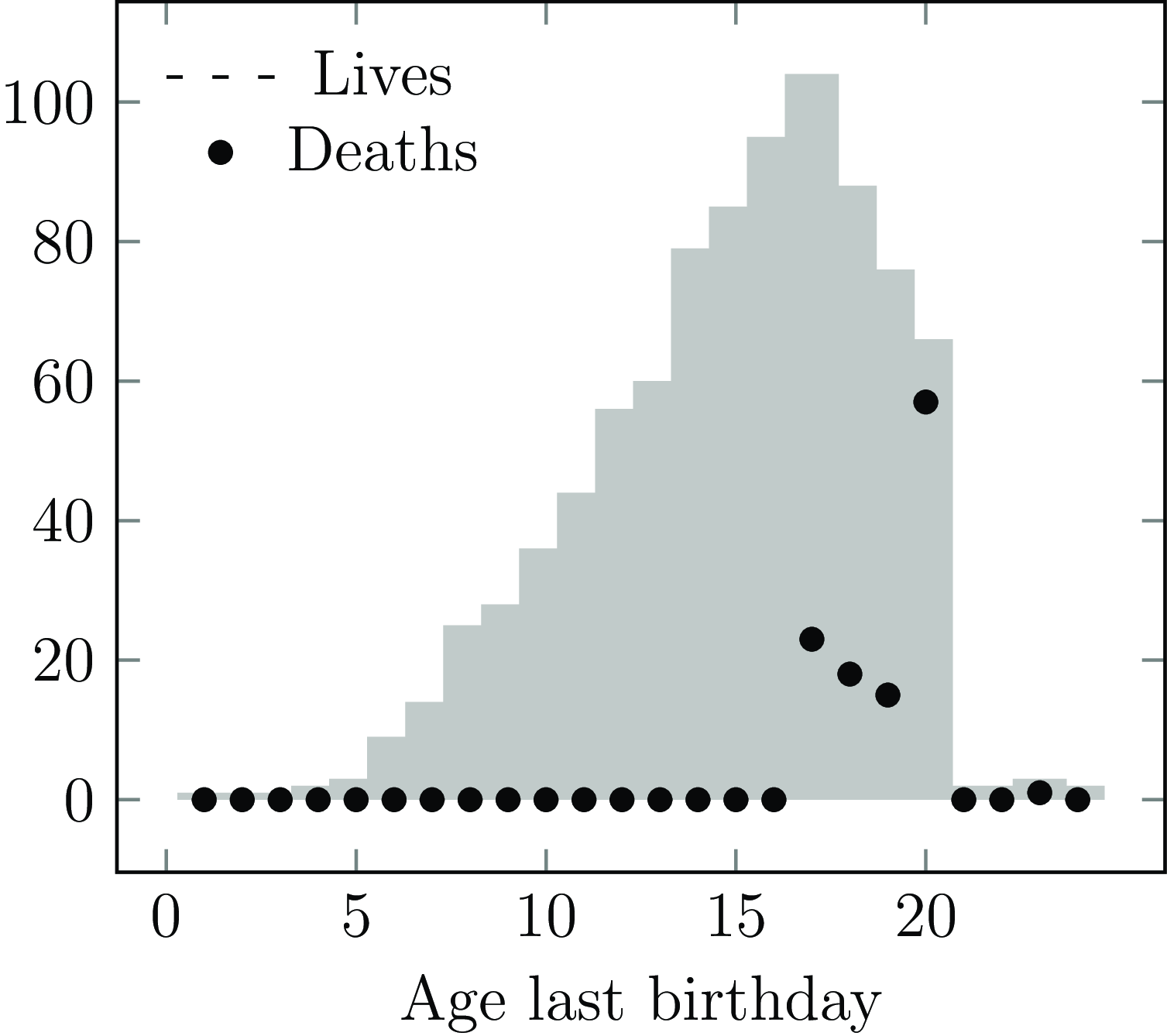
Mortality-only Kaplan-Meier survival curves for lives in a home-reversion portfolio with competing risks including long-term care inception, property buyback, voluntary surrender of lease and divorce.
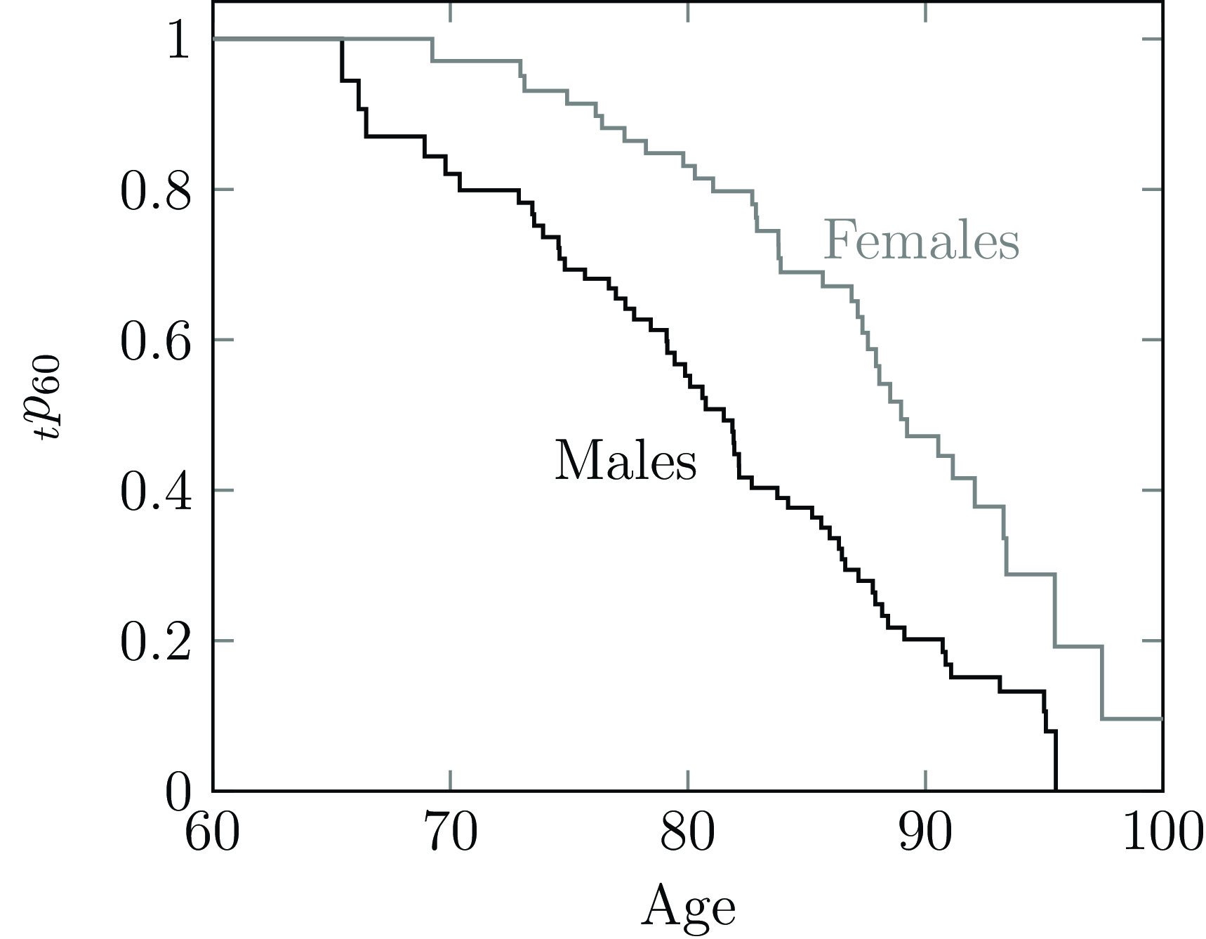
Case Study A.33
A reinsurer is invited to place a bid for a longevity swap. There are multiple bidders and there will be at least two rounds of bidding; the weakest bids in one round will be dropped from the next round of bidding. A data room is provided for all bidders, including mortality experience data for the portfolio concerned.
During analysis the reinsurer discovers a material issue with the data and asks for a corrected extract. The consultancy managing the bidding process refuses, saying that any updated data will only be provided in a later round. The reinsurer has a dilemma: if it prices too conservatively, it risks not being invited to the second round and never seeing the corrected data; however, if the reinsurer prices using the data as they are, there will be resistance to any unfavourable revision in price based on updated data. The reinsurer is also not entirely sure when (or even if) the cedant will provide updated data.
The reinsurer prices the bid using the data as they are, then decides on an adjustment in respect of the data problems. The reinsurer then communicates the pricing basis with the data-quality adjustment highlighted as a separate item. This makes it explicit to the cedant that there is a cost for poor data quality, and sets a measurable financial incentive to provide corrected data for the mortality experience.
B. Fractional Years of Exposure for Individual $q$
-Type Models
$q$
-Type Models

This appendix is about modelling mortality at the level of the individual. For simplicity we will mainly consider the problem of right-censored fractional years of exposure.
A recurring theme in this paper is that annual $q$
-type models of individual mortality typically require the analyst to discard fractional years of exposure. This is certainly true when using standard packaged models, such as GLMs; Figure B1 shows the trade-off available. Even if a likelihood cannot lead to a GLM it may still be perfectly useable as a model, see Macdonald and Richards (Reference Macdonald and Richards2025), Section 3.7.
$q$
-type models of individual mortality typically require the analyst to discard fractional years of exposure. This is certainly true when using standard packaged models, such as GLMs; Figure B1 shows the trade-off available. Even if a likelihood cannot lead to a GLM it may still be perfectly useable as a model, see Macdonald and Richards (Reference Macdonald and Richards2025), Section 3.7.
Trade-off decision tree for one-year $q$
-type models for individual lives. One cannot have both a GLM and fractional years of exposure.
$q$
-type models for individual lives. One cannot have both a GLM and fractional years of exposure.
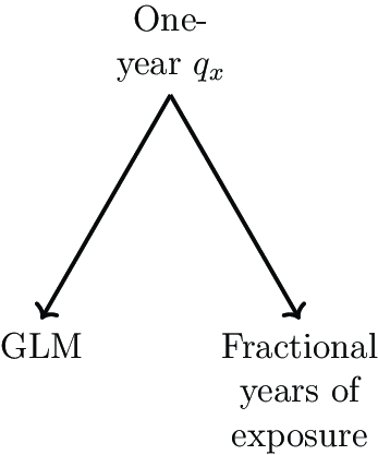
Note that the trade-offs with ${q_x}$
models go further than Figure B1. For example, an analyst may decide that she has sufficient data to not need fractional years of exposure, and so can use a GLM for a one-year
${q_x}$
models go further than Figure B1. For example, an analyst may decide that she has sufficient data to not need fractional years of exposure, and so can use a GLM for a one-year ${q_x}$
. However, this still means that she cannot simultaneously model period effects and selection effects, as described in Section 4.2.
${q_x}$
. However, this still means that she cannot simultaneously model period effects and selection effects, as described in Section 4.2.
In this appendix we explore some of the options available to a ${q_x}$
modeller for handling fractional years of exposure. As we will see, these options are incompatible with the use of a GLM, but they are achievable with a bespoke likelihood optimized in another way. However, if one is optimizing a likelihood directly, one might as well use a survival model.
${q_x}$
modeller for handling fractional years of exposure. As we will see, these options are incompatible with the use of a GLM, but they are achievable with a bespoke likelihood optimized in another way. However, if one is optimizing a likelihood directly, one might as well use a survival model.
In the rest of this appendix we have a single life aged $x$
that is observed for
$x$
that is observed for $t$
years with
$t$
years with $0 \lt t \lt 1$
.
$0 \lt t \lt 1$
. $d$
is an indicator variable taking the value 1 if the life is dead at age
$d$
is an indicator variable taking the value 1 if the life is dead at age $x + t$
and zero otherwise. We consider various ways of incorporating
$x + t$
and zero otherwise. We consider various ways of incorporating ${{\rm{\;}}_t}{q_x}$
into a likelihood, where
${{\rm{\;}}_t}{q_x}$
into a likelihood, where ${q_x}$
is the probability of death in a single year of age allowing for all risk factors.
${q_x}$
is the probability of death in a single year of age allowing for all risk factors.
B.1. Standard Bernoulli GLM Likelihood
When a single full year of exposure is present, the standard individual contribution to a Bernoulli log-likelihood, ${\ell ^{{\rm{GLM}}}}$
, is given in Table B1:
${\ell ^{{\rm{GLM}}}}$
, is given in Table B1:
Log-likelihoods for ${q_x}$
models, with and without allowance for fractional years of exposure
${q_x}$
models, with and without allowance for fractional years of exposure
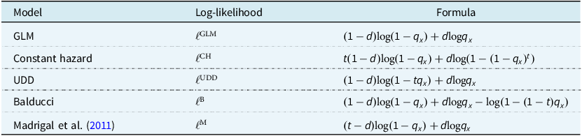
B.2. Constant Hazard
Under the constant-hazard assumption (Broffitt, Reference Broffitt1984, Table 1), $1{ - _t}{q_x} = {(1 - {q_x})^t}$
. The individual contribution to the Bernoulli log-likelihood,
$1{ - _t}{q_x} = {(1 - {q_x})^t}$
. The individual contribution to the Bernoulli log-likelihood, ${\ell ^{{\rm{CH}}}}$
, is given in Table B1. We can see from comparing GLM and CH log-likelihoods that the assumption of a constant hazard to allow for fractional years of exposure cannot be accommodated within a GLM because of the quite different form of the multiplier for
${\ell ^{{\rm{CH}}}}$
, is given in Table B1. We can see from comparing GLM and CH log-likelihoods that the assumption of a constant hazard to allow for fractional years of exposure cannot be accommodated within a GLM because of the quite different form of the multiplier for $d$
on the right.
$d$
on the right.
B.3. Uniform Distribution of Deaths (UDD)
Under the UDD assumption (Broffitt, Reference Broffitt1984, Table 1), ${{\rm{\;}}_t}{q_x} = t{q_x}$
. The individual contribution to the Bernoulli log-likelihood,
${{\rm{\;}}_t}{q_x} = t{q_x}$
. The individual contribution to the Bernoulli log-likelihood, ${\ell ^{{\rm{UDD}}}}$
, is given in Table B1. Note that we have dropped an additive term
${\ell ^{{\rm{UDD}}}}$
, is given in Table B1. Note that we have dropped an additive term ${t^d}$
as it does not involve the parameter
${t^d}$
as it does not involve the parameter ${q_x}$
, and so does not change inference. We can see from comparing the GLM and UDD log-likelihoods that the UDD allowance for fractional years of exposure cannot be accommodated within a GLM due to the presence of
${q_x}$
, and so does not change inference. We can see from comparing the GLM and UDD log-likelihoods that the UDD allowance for fractional years of exposure cannot be accommodated within a GLM due to the presence of $t$
in
$t$
in ${\rm{log}}\left( {1 - t{q_x}} \right)$
.
${\rm{log}}\left( {1 - t{q_x}} \right)$
.
B.4. Balducci Assumption
Also known as the hyperbolic assumption, the Balducci assumption is based on flawed reasoning (Hoem, Reference Hoem1984) and implies a decreasing hazard with age (Broffitt (Reference Broffitt1984), page 85 described the Balducci assumption as leading to “some unreasonable results”). It is therefore deprecated in favour of more realistic assumptions like the constant hazard or UDD. We include it here merely for historical curiosity; although it often appears in exercises for actuarial students, the Balducci assumption should never be used in real work. Under the Balducci assumption (Broffitt, Reference Broffitt1984, Table 1):
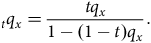 $${\;_t}{q_x} = {{t{q_x}} \over {1 - \left( {1 - t} \right){q_x}}}.$$
The contribution to the Bernoulli log-likelihood, ${\ell ^{\rm{B}}}$
, is given in Table B1. There is an additive
${\ell ^{\rm{B}}}$
, is given in Table B1. There is an additive ${t^d}$
term that does not affect inference for the parameter
${t^d}$
term that does not affect inference for the parameter ${q_x}$
and is therefore omitted. Once again, we can see from comparing the GLM and Balducci log-likelihoods that the Balducci assumption to allow for fractional years of exposure cannot be accommodated within a GLM because of the extra third term on the right of
${q_x}$
and is therefore omitted. Once again, we can see from comparing the GLM and Balducci log-likelihoods that the Balducci assumption to allow for fractional years of exposure cannot be accommodated within a GLM because of the extra third term on the right of ${\ell ^{\rm{B}}}$
.
${\ell ^{\rm{B}}}$
.
B.5. Weighting the Log-Likelihood
Madrigal et al. (Reference Madrigal, Matthews, Patel, Gaches and Baxter2011), Section 4.3.1 claimed that fractional years of exposure could be included in a $q$
-type model by “weight[ing] the contribution of each of the membership records according to its exposure to risk in a year.” However, this does not allow for fractional years of exposure, as discussed in Madrigal et al. (Reference Madrigal, Matthews, Patel, Gaches and Baxter2011), page 61. Madrigal et al. (Reference Madrigal, Matthews, Patel, Gaches and Baxter2011), page 62 claim that their individual contribution to the Bernoulli log-likelihood,
$q$
-type model by “weight[ing] the contribution of each of the membership records according to its exposure to risk in a year.” However, this does not allow for fractional years of exposure, as discussed in Madrigal et al. (Reference Madrigal, Matthews, Patel, Gaches and Baxter2011), page 61. Madrigal et al. (Reference Madrigal, Matthews, Patel, Gaches and Baxter2011), page 62 claim that their individual contribution to the Bernoulli log-likelihood, ${\ell ^{\rm{M}}}$
, is as given in Table B1 (after some re-arrangement). However,
${\ell ^{\rm{M}}}$
, is as given in Table B1 (after some re-arrangement). However, ${\ell ^{\rm{M}}}$
cannot be part of a GLM because of the
${\ell ^{\rm{M}}}$
cannot be part of a GLM because of the $\left( {t - d} \right)$
coefficient of
$\left( {t - d} \right)$
coefficient of ${\rm{log}}\left( {1 - {q_x}} \right)$
. Furthermore, weighting observations by the interval length is not a valid way to allow for fractional exposures.
${\rm{log}}\left( {1 - {q_x}} \right)$
. Furthermore, weighting observations by the interval length is not a valid way to allow for fractional exposures.
B.6. Modifying the data
For grouped-counts q-type models it would be possible to create an artificial equivalent number of lives to allow for less-than-complete years of exposure. This would typically involve a somewhat dubious assumption of a non-integer number of lives. However, this option makes little sense when modelling mortality at the level of individual lives.
B.7. Conclusions
As per Figure B1, the only way to have a one-year $q$
-type GLM is to discard fractional years of exposure. If the actuary insists on a
$q$
-type GLM is to discard fractional years of exposure. If the actuary insists on a $q$
-type model, but relaxes the requirement to have a GLM, then it is possible to directly use a likelihood with either the constant-hazard or UDD assumptions. Apparent alternatives are either deprecated (such as the Balducci assumption (Hoem, Reference Hoem1984)) or invalid (such as weighting the exposures as in Madrigal et al. (Reference Madrigal, Matthews, Patel, Gaches and Baxter2011, Section 4.3.1).
$q$
-type model, but relaxes the requirement to have a GLM, then it is possible to directly use a likelihood with either the constant-hazard or UDD assumptions. Apparent alternatives are either deprecated (such as the Balducci assumption (Hoem, Reference Hoem1984)) or invalid (such as weighting the exposures as in Madrigal et al. (Reference Madrigal, Matthews, Patel, Gaches and Baxter2011, Section 4.3.1).
However, a one-year $q$
-type model still involves compromises, such as the inability to simultaneously model period effects and selection effects demonstrated in Section 4.2. If an analyst is willing to directly maximize a likelihood, then a survival model for
$q$
-type model still involves compromises, such as the inability to simultaneously model period effects and selection effects demonstrated in Section 4.2. If an analyst is willing to directly maximize a likelihood, then a survival model for ${\mu _x}$
is both simpler and less restrictive.
${\mu _x}$
is both simpler and less restrictive.
B.8. Open-Source Software Implementations
The R (R Core Team, 2021) stats package contains the glm() function for fitting ordinary GLMs for $q$
-type and
$q$
-type and $\mu $
-type models. However,
$\mu $
-type models. However, $q$
-type GLMs can only be fitted where the exposure intervals are of identical length, i.e. no fractional years of exposure.
$q$
-type GLMs can only be fitted where the exposure intervals are of identical length, i.e. no fractional years of exposure.
C. Discarding Data
C.1. Background
Methods based on the estimation of ${q_x}$
came naturally in early studies of mortality, since the aim was to construct a life table. Notably, the seminal attempt to give an explanatory model of mortality (Gompertz, Reference Gompertz1825) was based on
${q_x}$
came naturally in early studies of mortality, since the aim was to construct a life table. Notably, the seminal attempt to give an explanatory model of mortality (Gompertz, Reference Gompertz1825) was based on ${\mu _x}$
, but this lead was pursued only sporadically in the following two centuries. Even in 1988, the landmark paper of its time (Forfar et al., Reference Forfar, McCutcheon and Wilkie1988) treated the estimation of
${\mu _x}$
, but this lead was pursued only sporadically in the following two centuries. Even in 1988, the landmark paper of its time (Forfar et al., Reference Forfar, McCutcheon and Wilkie1988) treated the estimation of ${\mu _x}$
and
${\mu _x}$
and ${q_x}$
equally. There are, of course, situations where the data make a binomial model most appropriate (see Case Study A.17 in Appendix A) but otherwise the
${q_x}$
equally. There are, of course, situations where the data make a binomial model most appropriate (see Case Study A.17 in Appendix A) but otherwise the $q$
-type modeller faces a choice between discarding data that do not suit the hypothesis, or adapting the hypothesis to suit the actual data.
$q$
-type modeller faces a choice between discarding data that do not suit the hypothesis, or adapting the hypothesis to suit the actual data.
When starting out in mortality studies, it is often stated, or simply assumed, that all data must be included in the analysis – that discarding some selected data must bias the results – thus presenting the $q$
-type modeller with a problem. However, this is rarely demonstrated, which is understandable, as doing so requires much of the apparatus which has not yet been seen. In this appendix, we consider the legitimacy of discarding parts of the data. Our approach is informal, drawing on the more formal arguments in Andersen et al. (Reference Andersen, Borgan, Gill and Keiding1993), which are based on counting processes. We refer the reader there for a more rigorous treatment.
$q$
-type modeller with a problem. However, this is rarely demonstrated, which is understandable, as doing so requires much of the apparatus which has not yet been seen. In this appendix, we consider the legitimacy of discarding parts of the data. Our approach is informal, drawing on the more formal arguments in Andersen et al. (Reference Andersen, Borgan, Gill and Keiding1993), which are based on counting processes. We refer the reader there for a more rigorous treatment.
For simplicity we confine attention to an interval of age $\left[ {x,x + 1} \right]$
, and suppress the initial age
$\left[ {x,x + 1} \right]$
, and suppress the initial age $x$
, so we consider the interval of time or duration
$x$
, so we consider the interval of time or duration $t \in \left[ {0,1} \right]$
. We assume a constant force of mortality
$t \in \left[ {0,1} \right]$
. We assume a constant force of mortality $\mu $
on this interval, therefore also a binomial model with parameter
$\mu $
on this interval, therefore also a binomial model with parameter $q = 1 - {\rm{exp}}\left( { - \mu } \right)$
. This is enough for our purpose because:
$q = 1 - {\rm{exp}}\left( { - \mu } \right)$
. This is enough for our purpose because:
-
(a) if
$\hat \mu $
is the maximum likelihood estimate of
$\mu $
then
$1 - {\rm{exp}}\left( { - \hat \mu } \right)$
is the maximum likelihood estimate of
$q$
; and -
(b) our analysis can be extended to non-constant parameters
${\mu _{x + t}}$
and
${q_{x + t}}$
but at the cost of much more notation and the use of product integrals (see Macdonald and Richards (Reference Macdonald and Richards2025)).


C.2. Data and Likelihood
We observe $M$
individuals, and for the
$M$
individuals, and for the $i$
th individual we have the following data:
$i$
th individual we have the following data:
-
(a) durations
${r_i}$
of entry to observation and
${t_i}$
of exit from observation, with
$0 \le {r_i} \lt {t_i} \le 1$
; and -
(b) an integer-valued indicator
${d_i}$
of the reason for observation ceasing;
${d_i} = 1$
if the reason was death, and
${d_i} = 0$
if the reason was right-censoring.


The $i$
th individual is observed on the interval
$i$
th individual is observed on the interval $\left[ {{r_i},{t_i}} \right]$
, which we denote by
$\left[ {{r_i},{t_i}} \right]$
, which we denote by ${{\rm{\Delta }}_i}$
, and we denote the interval
${{\rm{\Delta }}_i}$
, and we denote the interval $\left[ {0,1} \right]$
by
$\left[ {0,1} \right]$
by ${\rm{\Delta }}$
. From Macdonald and Richards (Reference Macdonald and Richards2025) we borrow the process
${\rm{\Delta }}$
. From Macdonald and Richards (Reference Macdonald and Richards2025) we borrow the process ${Y^i}\left( t \right)$
, equal to 1 if the
${Y^i}\left( t \right)$
, equal to 1 if the $i$
th individual is under observation “just before” time
$i$
th individual is under observation “just before” time $t$
, and equal to 0 otherwise (the “just before” is a technicality we can ignore).
$t$
, and equal to 0 otherwise (the “just before” is a technicality we can ignore).
To extend the model to allow for voluntary lapsation, all that is needed is to (i) assume that a constant force of lapsing $\nu $
operates alongside
$\nu $
operates alongside $\mu $
, and (ii) to define another indicator
$\mu $
, and (ii) to define another indicator ${w_i}$
, taking the value 1 if lapsing is the reason for observation ceasing, and 0 otherwise.
${w_i}$
, taking the value 1 if lapsing is the reason for observation ceasing, and 0 otherwise.
The contribution of the $i$
th individual to the likelihood is the factor
$i$
th individual to the likelihood is the factor ${L_i}$
defined as:
${L_i}$
defined as:
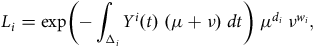 $${L_i} = {\rm{exp}}\left( { - \mathop \int \nolimits_{{{\rm{\Delta }}_i}} {Y^i}\left( t \right){\rm{\;}}\left( {\mu + \nu } \right){\rm{\;}}dt} \right){\rm{\;}}{\mu ^{{d_i}}}{\rm{\;}}{\nu ^{{w_i}}},$$
the total likelihood, denoted by $L$
, is:
$L$
, is:
 $$L = \mathop \prod \limits_i {L_i},$$
and the MLE, denoted by $\hat \mu $
, is:
$\hat \mu $
, is:
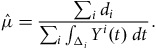 $$\hat \mu = {{\mathop \sum \nolimits_i {d_i}} \over {\mathop \sum \nolimits_i \mathop \int \nolimits_{{{\rm{\Delta }}_i}} {Y^i}\left( t \right){\rm{\;}}dt}}.$$
C.3. Obligate versus Random Right-Censoring
Observation of the $i$
th individual is left-truncated if
$i$
th individual is left-truncated if ${r_i} \gt 0$
. Observation is right-censored if
${r_i} \gt 0$
. Observation is right-censored if ${d_i} = 0$
, but we distinguish two kinds of right-censoring:
${d_i} = 0$
, but we distinguish two kinds of right-censoring:
-
(a) random right-censoring means the policy lapsed,
${w_i} = 1$
; and -
(b) obligate right-censoring means the individual was observed to survive until some predetermined time (in a sense to be made precise shortly) at which observation necessarily ended. Examples of such times are:
-
(1) the end of the interval
$\left[ {0,1} \right]$
(or more generally, the rate interval); -
(2) the date of data extraction;
-
(3) the date of transfer out of the portfolio; or
-
(4) the end date of the investigation.
-


The key point about obligate right-censoring is that the time of obligate right-censoring is known as soon as the individual enters observationFootnote
3
. Technically, the time $t'_i$
when observation on the
$t'_i$
when observation on the $i$
th individual must end is a random variable with
$i$
th individual must end is a random variable with ${r_i} \lt t'_i \le 1$
, but its value becomes known when the
${r_i} \lt t'_i \le 1$
, but its value becomes known when the $i$
th individual enters observation at time
$i$
th individual enters observation at time ${r_i}$
(that is,
${r_i}$
(that is, $t'_i$
is
$t'_i$
is ${\mathcal{F}_{{r_i}}}$
-measurable). So we have three possible cases:
${\mathcal{F}_{{r_i}}}$
-measurable). So we have three possible cases:
-
(a) Case 1: obligate right-censoring,
${d_i} = {w_i} = 0$
,
${t_i} = t'_i$
; -
(b) Case 2: random right-censoring,
${d_i} = 0$
,
${w_i} = 1$
,
${t_i} \lt t'_i$
; and -
(c) Case 3: death,
${d_i} = 1$
,
${w_i} = 0$
,
${t_i} \lt t'_i$
.


The main result of this Appendix is that the data on selected lives can be discarded, based on the time ${r_i}$
of entry and the time
${r_i}$
of entry and the time $t'_i$
of obligate right-censoring, without biasing the estimation of
$t'_i$
of obligate right-censoring, without biasing the estimation of $\mu $
. However, randomly right-censored data cannot be so discarded.
$\mu $
. However, randomly right-censored data cannot be so discarded.
Define ${\rm{\Delta'_i }} = \left[ {{r_i},t'_i} \right]$
, the greatest interval on which the
${\rm{\Delta'_i }} = \left[ {{r_i},t'_i} \right]$
, the greatest interval on which the $i$
th individual might be observed, and define
$i$
th individual might be observed, and define ${\rm{\Delta }} = \left[ {0,1} \right]$
. Then:
${\rm{\Delta }} = \left[ {0,1} \right]$
. Then:
-
(a) observation of the
$i$
th individual is randomly right-censored if
${w_i} = 1$
; and -
(b) observation of the
$i$
th individual is left-truncated or obligate right-censored if
${\rm{\Delta'_i }} \ne {\rm{\Delta }}$
.


C.4. Discarding Left-truncated and Obligate Right-censored Data
If ${\rm{\Delta'_i }} \ne {\rm{\Delta }}$
then the individual cannot complete a full year’s exposure. If the
${\rm{\Delta'_i }} \ne {\rm{\Delta }}$
then the individual cannot complete a full year’s exposure. If the $q$
-type analyst discards such data, the modified likelihood, denoted by
$q$
-type analyst discards such data, the modified likelihood, denoted by ${L^{{\rm{}}Obl{\rm{\;}}}}$
, is:
${L^{{\rm{}}Obl{\rm{\;}}}}$
, is:
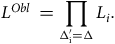 $${L^{{\rm{}}Obl{\rm{\;}}}} = \mathop \prod \limits_{{\rm{\Delta'_i }} = {\rm{\Delta }}} {L_i}.$$
Assuming that there is no selective reason for entry to be left-truncated or exit to be obligate right-censored, all such data can be discarded, deaths and lapses along with exposure data, without biasing any likelihood-based estimation. Note that this is an assumption that often seems reasonable, but may be hard to verify. Therefore:
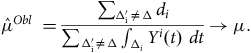 $${\hat \mu ^{{\rm{}}Obl{\rm{\;}}}} = {{\mathop \sum \nolimits_{{\rm{\Delta'_i }} \ne {\rm{\Delta }}} {d_i}} \over {\mathop \sum \nolimits_{{\rm{\Delta'_i }} \ne {\rm{\Delta }}} \mathop \int \nolimits_{{{\rm{\Delta }}_i}} {Y^i}\left( t \right){\rm{\;}}dt}} \to \mu .$$
See Section III.2.2, also Example III.2.3, in Andersen et al. (Reference Andersen, Borgan, Gill and Keiding1993) for a formal justification.
C.5. Discarding Randomly Right-censored Data
If randomly right-censored data are discarded the modified likelihood, denoted by ${L^{{\rm{Ran\;}}}}$
, is:
${L^{{\rm{Ran\;}}}}$
, is:
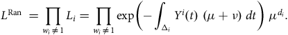 $${L^{{\rm{Ran\;}}}} = \mathop \prod \limits_{{w_i} \ne 1} {L_i} = \mathop \prod \limits_{{w_i} \ne 1} {\rm{exp}}\left( { - \mathop \int \nolimits_{{{\rm{\Delta }}_i}} {Y^i}\left( t \right){\rm{\;}}\left( {\mu + \nu } \right){\rm{\;}}dt} \right){\rm{\;}}{\mu ^{{d_i}}}.$$
If ${w_i} = 1$
and the
${w_i} = 1$
and the $i$
th individual’s data is excluded, the time
$i$
th individual’s data is excluded, the time $\left| {{{\rm{\Delta }}_i}} \right|$
for which the individual was exposed to the risk of death and lapse, is removed from the exposed-to-risk, but no deaths are removed from the data. The MLE
$\left| {{{\rm{\Delta }}_i}} \right|$
for which the individual was exposed to the risk of death and lapse, is removed from the exposed-to-risk, but no deaths are removed from the data. The MLE ${\hat \mu ^{\rm Ran{\rm{\;}}}}$
is:
${\hat \mu ^{\rm Ran{\rm{\;}}}}$
is:
 $${\hat \mu ^{\rm Ran{\rm{\;}}}} = {{\mathop \sum \nolimits_{{w_i} \ne 1} {d_i}} \over {\mathop \sum \nolimits_{{w_i} \ne 1} \mathop \int \nolimits_{{{\rm{\Delta }}_i}} {Y^i}\left( t \right){\rm{\;}}dt}} = {{\mathop \sum \nolimits_i {d_i}} \over {\mathop \sum \nolimits_{{w_i} \ne 1} \mathop \int \nolimits_{{{\rm{\Delta }}_i}} {Y^i}(t){\rm{\;}}dt}} \ge {{\mathop \sum \nolimits_i {d_i}} \over {\mathop \sum \nolimits_i \mathop \int \nolimits_{{{\rm{\Delta }}_i}} {Y^i}\left( t \right){\rm{\;}}dt}} = \hat \mu$$
where the last inequality is strict if and only if at least one individual lapses. Therefore, discarding randomly right-censored data will bias the estimate of $\mu $
upwards, and also the estimate of
$\mu $
upwards, and also the estimate of $q$
. Of course, the argument displayed in (C7) is exactly the same as the normal argument for not excluding censored data in a survival analysis.
$q$
. Of course, the argument displayed in (C7) is exactly the same as the normal argument for not excluding censored data in a survival analysis.
D. Non- and Semi-Parametric Methods
Between the worlds of discrete-time and continuous-time analysis lies a middle ground of non- and semi-parametric methods. These are based on occurrence-exposure ratios, but where the interval is neither fixed nor set by the analyst. Instead, the interval sizes are determined by the data, specifically the gaps between each death and the next. As the portfolio size grows, the gaps shrink to a single day, and thus non- and semi-parametric methods quickly become continuous-time methods for all practical purposes. Actuaries should not be confused by the $d/l$
notation for ratios into thinking that these are
$d/l$
notation for ratios into thinking that these are $q$
-type methodologies – the occurrence-exposure ratios are estimating mortality over short intervals, i.e. they are estimates of
$q$
-type methodologies – the occurrence-exposure ratios are estimating mortality over short intervals, i.e. they are estimates of $\mu $
.
$\mu $
.
In this appendix we look at three different methodologies for three different time dimensions: age, duration and calendar time. These methodologies have much to offer practising actuaries, from the data-quality checking of Section 7 to the real-time reporting of Section 8.
D.1. Kaplan-Meier Estimator
The methodology of Kaplan and Meier (Reference Kaplan and Meier1958) is non-parametric, and is a re-arrangement of the experience data into a survival curve. This survival curve can be by duration, such as is often the case with medical trials (Collett, Reference Collett2003, Section 2.1.2). However, the most useful definition of the Kaplan-Meier estimator for actuaries is the one by age in Macdonald et al. (Reference Macdonald, Richards and Currie2018, equation 8.3):
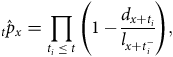 $${\;_t}{\hat p_x} = \prod\limits_{{t_i} \le t} {\left( {1 - {{{d_{x + {t_i}}}} \over {{l_{x + t_i^ - }}}}} \right)}, $$
where $x$
is the outset age for the survival function,
$x$
is the outset age for the survival function, $\left\{ {x + {t_i}} \right\}$
is the set of distinct ages at death,
$\left\{ {x + {t_i}} \right\}$
is the set of distinct ages at death, ${l_{x + t_i^ - }}$
is the number of lives alive immediately before age
${l_{x + t_i^ - }}$
is the number of lives alive immediately before age $x + {t_i}$
and
$x + {t_i}$
and ${d_{x + {t_i}}}$
is the number of deaths occurring at age
${d_{x + {t_i}}}$
is the number of deaths occurring at age $x + {t_i}$
. Informally, and following Section 2, we can think of
$x + {t_i}$
. Informally, and following Section 2, we can think of ${l_{x + t_i^ - }}$
as the number of lives alive just after midnight on a given day, with deaths
${l_{x + t_i^ - }}$
as the number of lives alive just after midnight on a given day, with deaths ${d_{x + {t_i}}}$
happening around mid-day. Figures 12(a) and A3 show examples of Kaplan-Meier curves.
${d_{x + {t_i}}}$
happening around mid-day. Figures 12(a) and A3 show examples of Kaplan-Meier curves.
The Kaplan-Meier estimator in Equation (D1) is the product-limit estimator of the survival curve discussed in Macdonald and Richards (Reference Macdonald and Richards2025), Section 4.2. It is also the product integral of the Nelson-Aalen estimator in Equation (D3).
D.2. Nelson-Aalen Estimator
The methodology of Nelson (Reference Nelson1958) is non-parametric, and is a re-arrangement of the experience data into a cumulative risk curve. This cumulative risk can be by duration, such as is often the case in medical studies:
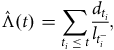 $$\hat \Lambda \left( t \right) = \sum\limits_{{t_i} \le t} {{{{d_{{t_i}}}} \over {{l_{t_i^ - }}}}}, $$
where $\left\{ {{t_i}} \right\}$
is the set of distinct durations at death,
$\left\{ {{t_i}} \right\}$
is the set of distinct durations at death, ${l_{t_i^ - }}$
is the number of lives alive immediately before duration
${l_{t_i^ - }}$
is the number of lives alive immediately before duration ${t_i}$
and
${t_i}$
and ${d_{{t_i}}}$
is the number of deaths occurring at duration
${d_{{t_i}}}$
is the number of deaths occurring at duration ${t_i}$
. Figure 14 shows an example of Equation (D2) being used to monitor differences in mortality for new annuity business.
${t_i}$
. Figure 14 shows an example of Equation (D2) being used to monitor differences in mortality for new annuity business.
However, another useful definition for actuaries is one by age:
 $${\hat \Lambda _x}\left( t \right) = \sum\limits_{{t_i} \le t} {{{{d_{x + {t_i}}}} \over {{l_{x + t_i^ - }}}}} .$$
The Nelson-Aalen estimator is the non-parametric estimator of the integrated hazard in Macdonald et al. (Reference Macdonald, Richards and Currie2018, equation 3.23).
D.3. Fleming-Harrington estimator
The methodology of Fleming and Harrington (Reference Fleming and Harrington1991) is non-parametric, and uses the Nelson-Aalen estimator of the cumulative hazard to estimate the survival curve from age $x$
:
$x$
:
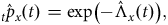 $${{\rm{\;}}_t}{\hat p_x} (t)= {\rm{exp}}\left( { - {{\hat \Lambda }_x}\left( t \right)} \right),$$
where ${\hat \Lambda _x}\left( t \right)$
is the Nelson-Aalen estimator from Equation (D3). The Fleming-Harrington estimator is the non-parametric equivalent of the identity:
${\hat \Lambda _x}\left( t \right)$
is the Nelson-Aalen estimator from Equation (D3). The Fleming-Harrington estimator is the non-parametric equivalent of the identity:
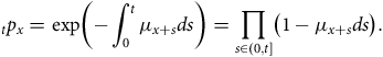 $${{\rm{\;}}_t}{p_x} = {\rm{exp}}\left( { - \mathop \int \nolimits_0^t {\mu _{x + s}}ds} \right) = \mathop \prod \limits_{s \in \left( {0,t} \right]} \left( {1 - {\mu _{x + s}}ds} \right).$$
The Fleming-Harrington estimator is slightly preferable to the Kaplan-Meier estimator for very small data sets, in part because approximate confidence intervals for the latter are not restricted to $\left[ {0,1} \right]$
(Collett, Reference Collett2003, Sections 2.2.1 and 2.2.3). However, for the data sets of the size that actuaries use there is usually no meaningful difference between the two estimators.
$\left[ {0,1} \right]$
(Collett, Reference Collett2003, Sections 2.2.1 and 2.2.3). However, for the data sets of the size that actuaries use there is usually no meaningful difference between the two estimators.
D.4. Relationships
There are important relationships between the Kaplan-Meier, Nelson-Aalen and Fleming-Harrington estimators. The product integral of a piecewise-constant function such as Equation (D3) is a discrete product such as Equation (D1). Therefore, the Kaplan-Meier estimator is the product integral of the Nelson-Aalen estimator; this is exact, not approximate. The Fleming-Harrington estimator in Equation (D4) is the exponential of (minus) the Nelson-Aalen estimator in Equation (D3), and is an approximation to the Kaplan-Meier estimator in Equation (D1) (and a good one for the datasets typically used by actuaries).
In some literature (SAS Institute Inc., 2017, page 5336) an alternative to Equation (D3) for small samples is given as:
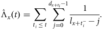 $${\hat \Lambda _x}\left( t \right) = \sum\limits_{{t_i} \le t} {\sum\limits_{j = 0}^{{d_{x + {t_i}}} - 1} {{1 \over {{l_{x + t_i^ - }} - j}}} } .$$
Equations (D3) and (D6) are identical if ${d_{x + {t_i}}} = 1$
. Even where some
${d_{x + {t_i}}} = 1$
. Even where some ${d_{x + {t_i}}}$
are greater than 1, Equation (D6) only produces materially different answers with small sample sizes. For actuarial data sets there is little meaningful difference, so we prefer Equation (D3) for simplicity.
${d_{x + {t_i}}}$
are greater than 1, Equation (D6) only produces materially different answers with small sample sizes. For actuarial data sets there is little meaningful difference, so we prefer Equation (D3) for simplicity.
D.5. Semi-parametric methods
Richards (Reference Richards2022b) introduced a semi-parametric estimator in calendar time for investigating short-term fluctuations in mortality. The methodology has two stages, the first of which is to calculate the non-parametric Nelson-Aalen estimator of the cumulative hazard with respect to calendar time, rather than age or duration:
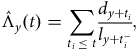 $${\hat \Lambda _y}\left( t \right) = \sum\limits_{{t_i} \le t} {{{{d_{y + {t_i}}}} \over {{l_{y + t_i^ - }}}}}, $$
where $y$
is the outset calendar time for the cumulative risk,
$y$
is the outset calendar time for the cumulative risk, $\left\{ {y + {t_i}} \right\}$
is the set of distinct dates of death,
$\left\{ {y + {t_i}} \right\}$
is the set of distinct dates of death, ${l_{y + t_i^ - }}$
is the number of lives alive immediately before date
${l_{y + t_i^ - }}$
is the number of lives alive immediately before date $x + {t_i}$
and
$x + {t_i}$
and ${d_{y + {t_i}}}$
is the number of deaths occurring on date
${d_{y + {t_i}}}$
is the number of deaths occurring on date $y + {t_i}$
. Informally, and following Section 2, we can think of
$y + {t_i}$
. Informally, and following Section 2, we can think of ${l_{y + t_i^ - }}$
as the number of lives alive just after midnight on a given day, with deaths
${l_{y + t_i^ - }}$
as the number of lives alive just after midnight on a given day, with deaths ${d_{y + {t_i}}}$
happening around mid-day.
${d_{y + {t_i}}}$
happening around mid-day. ${\hat \Lambda _y}\left( t \right)$
is the equivalent of Equation (D3), but with respect to calendar time instead of age. A practical point is that the real-valued calendar time is calculated using the actual number of days in the year, rather than the average of 365.24 given in Section 2. For example, 14th March 2023 would be represented as 2023.1973 (being 72 days into a 365-day year); in contrast, 14th March 2024 would be represented as 2024.1995 (being 73 days into a 366-day year).
${\hat \Lambda _y}\left( t \right)$
is the equivalent of Equation (D3), but with respect to calendar time instead of age. A practical point is that the real-valued calendar time is calculated using the actual number of days in the year, rather than the average of 365.24 given in Section 2. For example, 14th March 2023 would be represented as 2023.1973 (being 72 days into a 365-day year); in contrast, 14th March 2024 would be represented as 2024.1995 (being 73 days into a 366-day year).
The second step is to estimate the portfolio-level hazard in time, ${\mu _y}\left( t \right)$
. This ignores the age of individual lives, and so is only useful for investigating fluctuations over relatively short periods of time, where the age profile of the portfolio does not change radically. To estimate
${\mu _y}\left( t \right)$
. This ignores the age of individual lives, and so is only useful for investigating fluctuations over relatively short periods of time, where the age profile of the portfolio does not change radically. To estimate ${\mu _y}\left( t \right)$
from Equation (D7) we need to apply some degree of smoothing over a suitable short interval,
${\mu _y}\left( t \right)$
from Equation (D7) we need to apply some degree of smoothing over a suitable short interval, $c$
. We thus obtain a semi-parametric estimate of the mortality hazard at a point in time,
$c$
. We thus obtain a semi-parametric estimate of the mortality hazard at a point in time, ${\hat \mu _y}\left( {t,c} \right)$
, using
${\hat \mu _y}\left( {t,c} \right)$
, using $c$
as a bandwidth parameter. This can be done in a number of ways, but a simple one is to use a central difference in the estimator in Equation (D7) around the time of interest:
$c$
as a bandwidth parameter. This can be done in a number of ways, but a simple one is to use a central difference in the estimator in Equation (D7) around the time of interest:
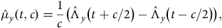 $${\hat \mu _y}\left( {t,c} \right) = {1 \over c}\left( {{{\hat \Lambda }_y}\left( {t + c/2} \right) - {{\hat \Lambda }_y}\left( {t - c/2} \right)} \right),$$
where $c$
is selected by the analyst to smooth random variation. When
$c$
is selected by the analyst to smooth random variation. When $c \le 0.5$
,
$c \le 0.5$
, ${\hat \mu _y}\left( {t,c} \right)$
will reveal detail such as seasonal variation (Figure 13(a)), mortality shocks (Richards, Reference Richards2022b, Figure 3) and data-quality issues (Figure 13(b) and (Richards, Reference Richards2022b, Appendix A)). When
${\hat \mu _y}\left( {t,c} \right)$
will reveal detail such as seasonal variation (Figure 13(a)), mortality shocks (Richards, Reference Richards2022b, Figure 3) and data-quality issues (Figure 13(b) and (Richards, Reference Richards2022b, Appendix A)). When $c \gg 0.5$
short-term variations are smoothed out. Over longer periods of time
$c \gg 0.5$
short-term variations are smoothed out. Over longer periods of time ${\hat \mu _y}\left( {t,c} \right)$
will reflect changes in the age distribution of the portfolio (Richards, Reference Richards2022b, Figure 2).
${\hat \mu _y}\left( {t,c} \right)$
will reflect changes in the age distribution of the portfolio (Richards, Reference Richards2022b, Figure 2).
Equation (D8) is calculated using an extract at a point in time, $u$
, so we could write
$u$
, so we could write ${\mu _y}\left( {t,c,u} \right)$
to make it explicit that the calculation is with respect to a particular data extract at time
${\mu _y}\left( {t,c,u} \right)$
to make it explicit that the calculation is with respect to a particular data extract at time $u$
. This can be useful when estimating delays in reporting deaths; see Section 4.3 and Richards (Reference Richards2022b), Section 4, where the ratio
$u$
. This can be useful when estimating delays in reporting deaths; see Section 4.3 and Richards (Reference Richards2022b), Section 4, where the ratio ${\mu _y}\left( {t,c,{u_1}} \right)/{\mu _y}\left( {t,c,{u_2}} \right)$
provides an estimate of the proportion of deaths reported up to time
${\mu _y}\left( {t,c,{u_1}} \right)/{\mu _y}\left( {t,c,{u_2}} \right)$
provides an estimate of the proportion of deaths reported up to time ${u_1}$
, under the assumption that the estimate at time
${u_1}$
, under the assumption that the estimate at time ${u_2}$
contains most of the unreported deaths up to time
${u_2}$
contains most of the unreported deaths up to time ${u_1}$
. This presupposes that the gap
${u_1}$
. This presupposes that the gap ${u_2} - {u_1}$
is large enough to allow most OBNR cases up to
${u_2} - {u_1}$
is large enough to allow most OBNR cases up to ${u_1}$
to have been subsequently reported. In reality, the estimate of
${u_1}$
to have been subsequently reported. In reality, the estimate of ${\mu _y}\left( {t,c,{u_2}} \right)$
at times before
${\mu _y}\left( {t,c,{u_2}} \right)$
at times before ${u_1}$
will also be affected by OBNR, but this effect can be minimized by a suitably large gap between
${u_1}$
will also be affected by OBNR, but this effect can be minimized by a suitably large gap between $u_1$
and
$u_1$
and ${u_2}$
.
${u_2}$
.
As an alternative to Equation (D8), ${\hat \mu _y}\left( {t,c} \right)$
could be calculated directly in a single step as:
${\hat \mu _y}\left( {t,c} \right)$
could be calculated directly in a single step as:
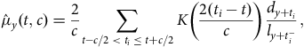 $${\hat \mu _y}\left( {t,c} \right) = {2 \over c}\mathop \sum \limits_{t - c/2 \lt {t_i} \le t + c/2} K\left( {{{2\left( {{t_i} - t} \right)} \over c}} \right){{{d_{y + {t_i}}}} \over {{l_{y + t_i^ - }}}},$$
where $K\left( u \right)$
is a kernel function for smoothing; see Andersen et al. (Reference Andersen, Borgan, Gill and Keiding1993), Section IV.2.1. Equation (D8) results from using the uniform kernel:
$K\left( u \right)$
is a kernel function for smoothing; see Andersen et al. (Reference Andersen, Borgan, Gill and Keiding1993), Section IV.2.1. Equation (D8) results from using the uniform kernel:
 $$K\left( u \right) = \left\{ {\matrix{ {{1 \over 2}} & {\left| u \right| \le 1} \cr 0 & {{\rm{otherwise}},} \cr } } \right.$$
but other kernel smoothers with greater efficiency are available, such as the Epanechnikov kernel (Epanechnikov, Reference Epanechnikov1969):
 $$K\left( u \right) = \left\{ {\matrix{ {{3 \over 4}\left( {1 - {u^2}} \right)} & {\left| u \right| \le 1} \cr 0 & {{\rm{otherwise}}.} \cr } } \right.$$
The kernel functions in Equations (D10) and (D11) are illustrated in Figure D1. The Epanechnikov kernel is more suitable for applications where measuring short-term fluctuations is important.

D.6. Open-source software implementations
The R (R Core Team, 2021) survival package contains the survfit() function for computing the Kaplan-Meier and Fleming-Harrington estimators in Equations (D3) and (D6). The Python module scikit-survival contains an implementation of the Kaplan-Meier estimator. However, many software implementations of Kaplan-Meier cannot handle left truncation by age, which is essential for actuarial work. The R script in Figure D2 can be used as an alternative, as it handles left truncation.
R script for non-parametric estimates with left-truncated data by age.
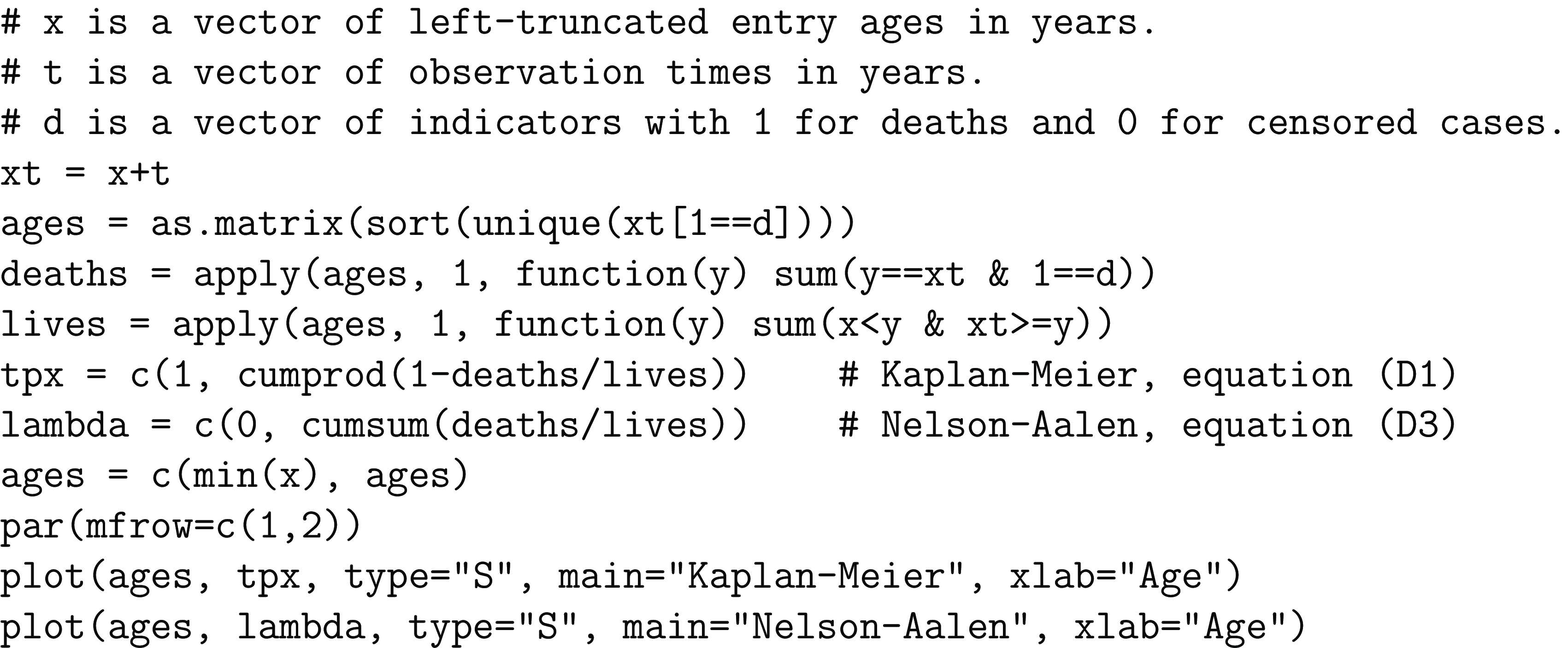
Richards (Reference Richards2022b), Appendix C contains R source code for the semi-parametric estimator in Equation (D8).
E. Individual lifetimes versus grouped counts
In the body of the paper we show why $\mu $
-type methods are superior to
$\mu $
-type methods are superior to $q$
-type methods. We also assume that individual records are extracted, as this enables better data-quality checking (Macdonald et al., Reference Macdonald, Richards and Currie2018, Chapter 2). However, the analyst still had two choices for a
$q$
-type methods. We also assume that individual records are extracted, as this enables better data-quality checking (Macdonald et al., Reference Macdonald, Richards and Currie2018, Chapter 2). However, the analyst still had two choices for a $\mu $
-type model: the modelling of individual lifetimes (a survival model) or the modelling of grouped counts.
$\mu $
-type model: the modelling of individual lifetimes (a survival model) or the modelling of grouped counts.
E.1. Individual lifetimes
Suppose we have the following for life $i$
: the entry age into observation,
$i$
: the entry age into observation, ${x_i}$
; the time observed,
${x_i}$
; the time observed, ${t_i}$
; and the indicator,
${t_i}$
; and the indicator, ${d_i}$
, which takes the value 1 if life
${d_i}$
, which takes the value 1 if life $i$
died at age
$i$
died at age ${x_i} + {t_i}$
and zero otherwise. The contribution,
${x_i} + {t_i}$
and zero otherwise. The contribution, ${L_i}$
, of life
${L_i}$
, of life $i$
to the likelihood is then:
$i$
to the likelihood is then:
 $${L_i}{ = _{{t_i}}}{p_{{x_i}}}\mu _{{x_i} + {t_i}}^{{d_i}}$$
 $$ = {\rm{exp}}\left( { - \mathop \int \nolimits_0^{{t_i}} {\mu _{{x_i} + s}}ds} \right)\mu _{{x_i} + {t_i}}^{{d_i}}$$
 $$ = {e^{ - {{\rm{\Lambda }}_{{x_i}}}\left( {{t_i}} \right)}}\mu _{{x_i} + {t_i}}^{{d_i}},$$
where ${{\rm{\Lambda }}_x}\left( t \right) = \mathop \int \nolimits_0^t {\mu _{x + s}}ds$
is the integrated hazard; see Macdonald et al. (Reference Macdonald, Richards and Currie2018, equation 3.23). The corresponding contribution of life
${{\rm{\Lambda }}_x}\left( t \right) = \mathop \int \nolimits_0^t {\mu _{x + s}}ds$
is the integrated hazard; see Macdonald et al. (Reference Macdonald, Richards and Currie2018, equation 3.23). The corresponding contribution of life $i$
to the log-likelihood,
$i$
to the log-likelihood, ${\ell _i}$
, is:
${\ell _i}$
, is:
 $${\ell _i} = {\rm{log}}{\,}{L_i}$$
 $$= - {{\rm{\Lambda }}_{{x_i}}}\left( {{t_i}} \right) + {d_i}{\,}{\rm{log}}{\mu _{{x_i} + {t_i}}}.$$
For a data set of $n$
lives, the full likelihood is then
$n$
lives, the full likelihood is then $L = \mathop \prod \nolimits_{i = 1}^n {L_i}$
and the corresponding log-likelihood is
$L = \mathop \prod \nolimits_{i = 1}^n {L_i}$
and the corresponding log-likelihood is $\ell = \mathop \sum \nolimits_{i = 1}^n {\ell _i}$
. Modelling individual lifetimes is the most elemental mortality model; Macdonald and Richards (Reference Macdonald and Richards2025) call this a “micro” model. One benefit of modelling individual lifetimes is that more information can be used on individual attributes and covariates. For example, Richards (Reference Richards2022a) showed how to include the exact pension amount as a continuous covariate in mortality modelling.
$\ell = \mathop \sum \nolimits_{i = 1}^n {\ell _i}$
. Modelling individual lifetimes is the most elemental mortality model; Macdonald and Richards (Reference Macdonald and Richards2025) call this a “micro” model. One benefit of modelling individual lifetimes is that more information can be used on individual attributes and covariates. For example, Richards (Reference Richards2022a) showed how to include the exact pension amount as a continuous covariate in mortality modelling.
E.2. Grouped counts
An alternative approach is to create homogeneous sub-groups of shared characteristics. Suppose for sub-group $j$
we have
$j$
we have ${n_j}$
lives with total time observed
${n_j}$
lives with total time observed $E_j^c = \mathop \sum \nolimits_{i = 1}^{{n_j}} {t_i}$
and total observed deaths
$E_j^c = \mathop \sum \nolimits_{i = 1}^{{n_j}} {t_i}$
and total observed deaths ${D_j} = \mathop \sum \nolimits_{i = 1}^{{n_j}} {d_i}$
. Assuming a constant mortality hazard rate of
${D_j} = \mathop \sum \nolimits_{i = 1}^{{n_j}} {d_i}$
. Assuming a constant mortality hazard rate of ${\mu _j}$
, the contribution to the likelihood,
${\mu _j}$
, the contribution to the likelihood, ${L_j}$
, is:
${L_j}$
, is:
 $${L_j} = {e^{ - E_j^c{\mu _j}}}\mu _j^{{D_j}}.$$
Equation (E6) looks like a Poisson likelihood, and this leads to the common misconception that ${D_j}$
has a Poisson distribution with mean parameter
${D_j}$
has a Poisson distribution with mean parameter $E_j^c{\mu _j}$
. This is not true, as demonstrated in detail by Macdonald and Richards (Reference Macdonald and Richards2025), Section 3. In fact, the random variable is the pair
$E_j^c{\mu _j}$
. This is not true, as demonstrated in detail by Macdonald and Richards (Reference Macdonald and Richards2025), Section 3. In fact, the random variable is the pair $\left( {{D_{}},E_j^c} \right)$
, which cannot have a Poisson distribution. However, the likelihoods for a Poisson model for
$\left( {{D_{}},E_j^c} \right)$
, which cannot have a Poisson distribution. However, the likelihoods for a Poisson model for ${D_j}$
and the pair
${D_j}$
and the pair $\left( {{D_j},E_j^c} \right)$
are the same up to a multiplicative constant, so the inference will be the same; Macdonald and Richards (Reference Macdonald and Richards2025), Section 3 called the likelihood in Equation (E6) pseudo-Poisson. This means that a pseudo-Poisson grouped-count model like Equation (E6) can be fitted using the machinery of a Poisson GLM, even though the observed death count
$\left( {{D_j},E_j^c} \right)$
are the same up to a multiplicative constant, so the inference will be the same; Macdonald and Richards (Reference Macdonald and Richards2025), Section 3 called the likelihood in Equation (E6) pseudo-Poisson. This means that a pseudo-Poisson grouped-count model like Equation (E6) can be fitted using the machinery of a Poisson GLM, even though the observed death count ${D_j}$
is not Poisson.
${D_j}$
is not Poisson.
Grouped-count models lose information due to grouping. Care is required with the assumption of a constant hazard rate, ${\mu _j}$
, which requires that lifetimes are split into small enough age ranges for this approximation to be justified; see Macdonald and Richards (Reference Macdonald and Richards2025), Appendix A. Even greater care is required with continuous variables like pension size, where the assumption of a constant effect within a discrete band can lead to systematic over-estimation of mortality of pensioners. Figure E1 shows the deviance residuals by pension size-band for a model with age and sex as covariates. The non-random variation suggests that the wealthiest pensioners have significantly lower mortality. If we split the lives into twenty equal-sized groups, Figure E1(a) suggests that the top 10% of amounts are different from the rest. However, Figure E1(c) shows that the assumption of a constant mortality effect within this group is false – there is continuous variation by pension amount. This is important for actuarial purposes, because the assumption of a constant effect risks financial bias – all other factors held equal, the financial impact of those on the right always outweighs the financial impact of those on the left.
${\mu _j}$
, which requires that lifetimes are split into small enough age ranges for this approximation to be justified; see Macdonald and Richards (Reference Macdonald and Richards2025), Appendix A. Even greater care is required with continuous variables like pension size, where the assumption of a constant effect within a discrete band can lead to systematic over-estimation of mortality of pensioners. Figure E1 shows the deviance residuals by pension size-band for a model with age and sex as covariates. The non-random variation suggests that the wealthiest pensioners have significantly lower mortality. If we split the lives into twenty equal-sized groups, Figure E1(a) suggests that the top 10% of amounts are different from the rest. However, Figure E1(c) shows that the assumption of a constant mortality effect within this group is false – there is continuous variation by pension amount. This is important for actuarial purposes, because the assumption of a constant effect risks financial bias – all other factors held equal, the financial impact of those on the right always outweighs the financial impact of those on the left.
Deviance residuals by pension size-band, with 1 representing the smallest pensions.
Source: Mortality model for age and sex for English pension scheme from Richards (Reference Richards2022a).
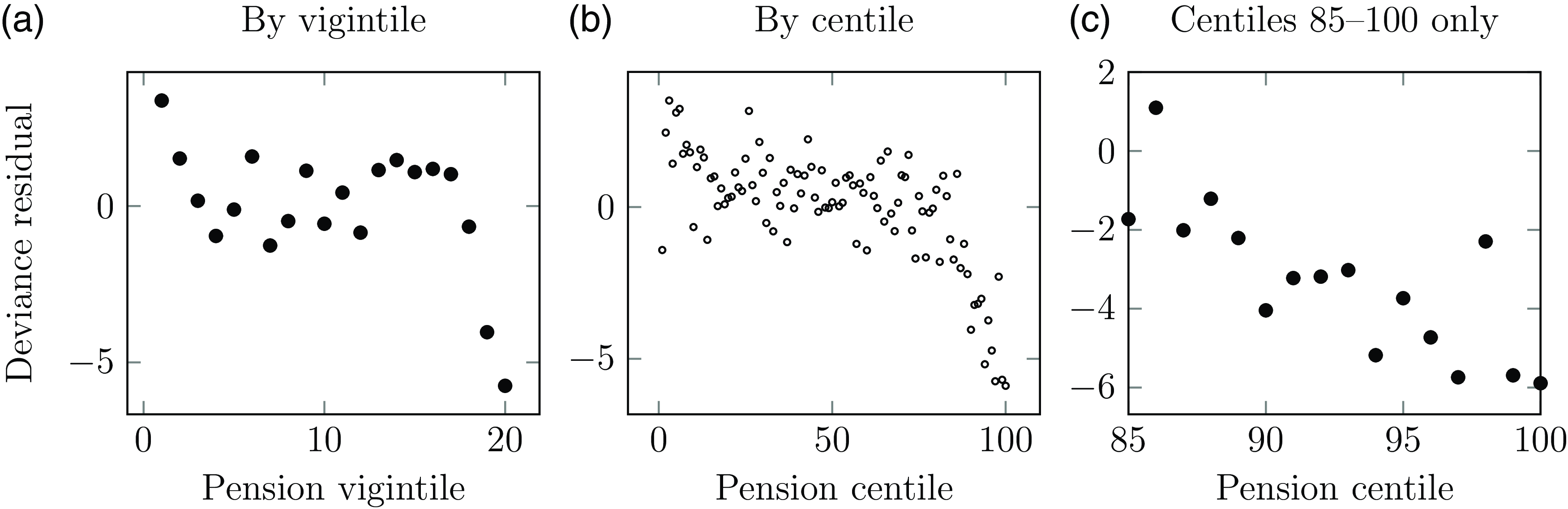
One counter-argument sometimes advanced in favour of discretization is that a model could be fitted using the 100 size-bands in Figure E1(b), say with some penalty function to dampen the inevitable volatility in parameter estimates. However, this would be an additional complexity to deal with the problem caused by discretization. It is far simpler to instead treat variables like pension size continuously and not have the problem arise in the first place. Richards (Reference Richards2022a), Tables 7 and 8 showed that treating pension amount as a continuous risk factor for mortality produced a model with the fewest parameters and the lowest-equal information criterion. This is an extension of graduation by mathematical formula, where a smooth progression in mortality rates by age is guaranteed during the model fit (Forfar et al., Reference Forfar, McCutcheon and Wilkie1988). We go a step further and treat all continuous variables this way, not just age.
E.3. Stratification
Irrespective of whether mortality modelling is of individual lifetimes or groups, there is the question of how to handle sub-groups with shared characteristics. One approach is to sub-divide the experience data and fit separate models, i.e. stratification of the data set. In general stratification should be avoided wherever possible, as it increases the overall number of parameters required and weakens the statistical power of the data set (Macdonald et al., Reference Macdonald, Richards and Currie2018, Section 7.3). However, stratification can on rare occasions be justified where the mortality hazard rate has fundamentally different properties, such as where sub-groups have a different shape of mortality curve by age.
E.4. Open-source software for individual lifetimes
The R (R Core Team, 2021) survival package contains the survreg() function for fitting parametric survival models. However, most of the models available do not handle left truncation. Macdonald et al. (Reference Macdonald, Richards and Currie2018), Chapter 5 provide R scripts for fitting models to left-truncated data, with discussion on use of the R’s nlm() and solve() functions. Commercially supported services are also available.


 Open access