


1. Introduction
Agricultural export is very crucial for the U.S. economy. Agricultural exports directly contributed around $175.5 billion to the U.S. economy in 2023 and generated an additional $186.9 billion in economic activity (USDA-ERS, 2025a). Furthermore, U.S. agricultural exports supported 1.05 million civilian jobs, including 582,870 jobs in non-farm sectors, and more specifically, each $1 billion of agricultural exports supported approximately 5,997 jobs (USDA-ERS, 2025a). However, despite having such importance in the national economy and being a net agricultural exporter nearly for 60 years in the global market until 2019, the United States is currently facing a structural challenge in its agricultural export strategy – an overconcentration in a limited number of markets (USDA-ERS, 2025b). On average, about 60% of the U.S. agricultural exports go to only five countries, namely China, Mexico, Canada, Japan, and South Korea (USDA-FAS, 2024). This overreliance on fewer markets makes the United States vulnerable to trade disputes. For example, because of the retaliatory tariff war with its major trading partners during 2018–19, the U.S. agricultural exports declined sharply and incurred losses of more than $27 billion, where 95% of the loss was attributed only to China (Morgan et al., Reference Morgan, Arita, Beckman, Ahsan, Russell, Jarrell and Kenner2022).
Simultaneously, the emergence of other countries, such as Brazil and Argentina, as major agricultural traders in the international export market is also posing challenges to the leadership position of the United States. For instance, Brazil became the world’s leading soybean exporters in 2013 surpassing the United States for the first time, and now Brazil is projected to have an increased market share from 51.6% to 60.6% between the marketing years 2021/22 to 2032/33, whereas the U.S. share is projected to drop from 38 to 28% (Valdes et al., Reference Valdes, Gillespie and Dohlman2023). Additionally, Brazil and Argentina’s increasing competitiveness in the world market is also partly contributing to a decline in the U.S. cotton and sorghum market share in recent times (Ghose et al., Reference Ghose and Hudson2025; Padilla et al., Reference Padilla, Ufer, Morgan and Link2023). Furthermore, China, the largest U.S. agricultural export market, began to diversify agricultural import sources outside of the United States since 2015, which is also concerning for the U.S. agricultural export sector (Hejazi et al., Reference Hejazi, Marchant, Zhu and Ning2019).
Considering the sector’s value to the economy, the U.S. government officials and policy experts prioritized diversifying U.S. agricultural export markets to prevent market-specific shocks and reliance on any one single dominant trading partner, such as China (Lee and Jones, Reference Lee and Jones2023). Wang and Liu (Reference Wang and Liu2023) supported the view of export market diversification because diversification has a lesser chance of being interrupted, and it helps to achieve greater success in expanding global market share. Analyzing Chinese firm-level data, Xuefeng and Yaşar (Reference Xuefeng and Yaşar2016) also confirmed diversification as a strategic tool for firms to internalize external shocks and improve performance, as they found a positive effect of export diversification on long-run average cost and productivity.
Hence, to develop a U.S. export strategy, the United States needs to identify potential new markets and analyze their prospects for agricultural trade. Because the emerging economies (specifically in South Asia, Southeast Asia, and Southern Africa) are experiencing rapid urbanization, demographic growth, and increasing income, these countries have rising demand for agricultural products compared to high-income economies such as Japan, Canada, and the EU where population and economic growth is sluggish and demand for agricultural product is flat (Regmi, Reference Regmi, Croft, Greene, Johnson and Schnepf2021; USDA-FAS, 2021b). However, several studies and institutional reports have found South AsianFootnote 1 and Southeast AsianFootnote 2 countries’ potential for U.S. agricultural exports based on their increasing population growth, rising per capita incomes, expanding middle classes, and rising demands for value-added agri-foods, especially the health and wellness segments (Regmi, Reference Regmi, Croft, Greene, Johnson and Schnepf2021; Sabala and Gale, Reference Sabala and Gale2025; Lee and Jones, Reference Lee and Jones2023). Likewise, Southern AfricaFootnote 3 , home to more than 167 million people and a region of growing upper-middle-income economies, imported $14 billion worth of agricultural goods from the United States in 2017, which is about 4% of its total imports (Southeast AgNet, 2018; Johnson et al., Reference Johnson, Morgan and Farris2023). Therefore, Southern Africa can be considered a promising agricultural export destination for the U.S. with promising export market potential.
The determinants of trade are not one-dimensional in nature, and hence, the selection of a suitable analytical model is crucial (Ebaidalla & Yahia, Reference Ebaidalla and Yahia2014; Stack and Pentecost, Reference Stack and Pentecost2011; Stack et al., Reference Stack, Pentecost and Ravishankar2018). The Stochastic Frontier Gravity Model (SFGM) has been demonstrated to measure trade potential and efficiency by differentiating the structural determinants from trade inefficiencies in different country contexts, i.e., China, Pakistan, Vietnam, and India, with important policy implications (Kalirajan, Reference Kalirajan2007; Ebaidalla and Yahia, Reference Ebaidalla and Yahia2014; Stack and Pentecost, Reference Stack and Pentecost2011; Stack et al., Reference Stack, Pentecost and Ravishankar2018; Romyen et al., Reference Romyen, Nunti and Neranon2023; Abdullahi et al., Reference Abdullahi, Zhang, Shahriar, Irshad, Ado, Huo and Zúniga-González2022). However, the stochastic frontier gravity model has not been utilized yet to analyze the potential for U.S. agricultural exports to South Asia, Southeast Asia, and Southern Africa, despite these three regions having favorable demographic and macroeconomic prospects. Thus, this study contributes to existing literature in two ways. First, this is the first study to apply SFGM specifically to these three underexplored but high-potential regions within the context of U.S. agricultural exports. Second, it calculates the export gap (the difference between potential and actual trade) and provides a framework for identifying and prioritizing target countries where the U.S. can undertake an effective export strategy and implement policy interventions to unlock its untapped market potential.
2. Literature review
Unobserved trade frictions and inefficiencies are not taken into consideration by traditional gravity models. Due to its ability to estimate both actual trade flows and possible trade optimal conditions, the SFGM overcomes these limitations. Inefficiencies caused by different institutional and structural barriers are also taken into account by SFGM. Armstrong (Reference Armstrong2007) argued that SFGM measures trade inefficiency as the difference between the trade frontier and actual trade. Therefore, the definition of potential trade in the SFGM framework would then be the highest level of trade attainable in the most favorable conditions, i.e., free-trade policies, sound institutions, and low resistance. Subsequent studies have also confirmed the SFGM to be a good method for capturing the efficiency of trade.
Ravishankar and Stack (Reference Ravishankar and Stack2014) analyzed 10 Eastern and 17 Western European countries’ trade integration between 1994 and 2007 using SFGM, and they revealed that trade had made significant progress in East–West integration to a level that had attained virtually two-thirds of its potential. Similarly, Stack and Pentecost (Reference Stack and Pentecost2011) studied trade potential between 20 OECD and EU countries from 1992 to 2003 and revealed that actual trade volumes of new EU member states were significantly below their projected potential. They pointed to considerable opportunities for expansion in the new EU member countries, in contrast to Mediterranean countries, which were found to be trading near their potential level. Together, these studies demonstrate the usefulness of the SFGM framework in quantifying trade inefficiencies and identifying gaps between observed and potential trade across different regional contexts.
Stochastic frontier gravity models have been applied in different countries and regional contexts to examine the determinants of bilateral trade and to estimate trade potential. While analyzing trade between Australia and countries around the Indian Ocean, Kalirajan (Reference Kalirajan2007) found that institutional and policy constraints were more significant in producing inefficiencies than geographic and economic factors, and regional cooperation increased trade efficiency by 15%. Ebaidalla and Yahia (Reference Ebaidalla and Yahia2014) found that despite having lower trade efficiency than ASEAN, the Common Market for Eastern and Southern Africa (COMESA) region was gradually catching up to ASEAN’s levels. Binh et al., (Reference Binh, Nguyen and Cuong2014) showed that Vietnam’s bilateral trade has enormous unrealized potential in both Western Asia and Africa, and its economic size, distance, and cultural affinities are all significant determinants of this trade. While assessing the potential of Pakistan for trade in South Asia, Masood et al., (Reference Masood, Khurshid, Haider, Khurshid and Khokhar2022) determined that the highest potential markets for Pakistan were Bangladesh, Nepal, and India, and they also determined policy reform to reduce tariff and non-tariff barriers to trade. These regional studies collectively highlight that trade inefficiencies are often driven by institutional, policy, and structural constraints rather than purely geographic factors.
Similarly, Abdullahi et al., (Reference Abdullahi, Huo, Zhang and Azeez2021) conducted a study on China’s agricultural exports with 114 nations from 2000 and 2019 using the SFGM, and they found that trade was positively impacted by economic size, the Belt and Road Initiative, shared borders, and language, but negatively impacted by distance, being landlocked, and currency devaluation. They also highlighted that China’s agri-food exports were utilizing only 49% of its potential, so there is scope for growth. Hajivand et al., (Reference Hajivand, Moghaddasi, Zeraatkish and Mohammadinejad2020) examined Iran’s agricultural trade with 38 nations between 1982 and 2017. They found that Iran’s GDP and population were the major drivers of exports, and Iran had only utilized 69% of its trade capacity. In the case of Pakistan again, Atif et al., (Reference Atif, Liu and Mahmood2016) concluded that Pakistan had a lot of unused agricultural export capacity, particularly in regional and Middle Eastern markets, and identified GDP, exchange rates, and sharing a common border and colonial past as the most important drivers of trade. Romyen et al., (Reference Romyen, Nunti and Neranon2023) used a copula-based gravity model to analyze Thailand’s agricultural export efficiency under different free trade agreements and found that these agreements have a positive effect on exports.
Overall, it is evident by a vast body of literature that stochastic frontier gravity model is successfully used in determining export potential of many countries and region in different context, but its application to the U.S. case has been limited so far. Therefore, our study filled this gap and utilized stochastic frontier gravity model to determine the untapped export potential of U.S. agricultural products to other potential countries.
3. Methodology and data
3.1. Stochastic frontier gravity model (SFGM)
The standard gravity model was widely used before 2000 in trade analysis for estimating the average effects of the trade determinants (Möhlmann et al., Reference Möhlmann, Ederveen, De Groot and Linders2010). Because the conventional gravity model typically uses average exports or imports of the trading countries rather than optimal exports or imports, Ravishankar and Stack (Reference Ravishankar and Stack2014) revealed that such averaging can mask the actual economic dynamics of trade between countries with a trade capacity much larger than another country. While the standard gravity model can capture observable barriers like distance, tariffs, etc., it is less effective in addressing subjective and unobservable barriers, such as sociopolitical and institutional constraints, which are important but difficult to measure (Armstrong, Reference Armstrong2007; Kalirajan, Reference Kalirajan2007). The unobservable barriers can pose significant challenges in trade analysis, leading to heteroskedastic errors because of these omitted variables (Kalirajan and Findlay, Reference Kalirajan and Findlay2005). Considering these limitations and addressing general-equilibrium consistency in trade modeling, Anderson and Wincoop (Reference Anderson and Van Wincoop2003) introduced the structural gravity model by incorporating multilateral resistance terms (MRTs) to account for the general equilibrium effects of trade barriers. MRTs capture how bilateral trade depends on relative trade costs across all trading partners, and empirical studies commonly approximate MRTs using exporter and importer fixed effects (Feenstra, Reference Feenstra2002; Choi et al., Reference Choi, Acharya, Devadoss and Regmi2024; Head and Mayer, Reference Head and Mayer2014). The structural gravity model incorporating MRTs is given by:
 $${AGRIE{X_{ijt}} = {{GD{P_{it}}GD{P_{jt}}} \over {GD{P_{wt}}}}{\left( {{{{T_{ij}}} \over {{P_i}{P_j}}}} \right)^{1 - \sigma }}}$$
where GDP it is the exporter i’s GDP, GDP jt is the importer j’s GDP, GDP wt is the world GDP, T ij denotes bilateral trade costs, P i and P j are the multilateral resistance indices for countries iand j, and σ > 1 is the elasticity of substitution. The terms P i and P j are implicit price indices reflecting market access conditions based on trade costs with all partners. This empirical strategy absorbs country-level resistance factors but does not mechanically eliminate bilateral trade-cost variables such as geographic distance, landlocked status, or common language (Head and Mayer, Reference Head and Mayer2014). Therefore, the structural gravity model is well-suited and frequently used in estimating trade policy impact and counterfactual analyses (Ridley et al., Reference Ridley, Luckstead and Devadoss2024; Ridley & Devadoss, Reference Ridley and Devadoss2023; Yotov et al., Reference Yotov, Piermartini, Monteiro and Larch2016; Yotov, Reference Yotov2022; Dhoubhadel and Ridley, Reference Dhoubhadel and Ridley2024; Dhoubhadel et al., Reference Dhoubhadel, Ridley and Devadoss2023).
However, while structural gravity models with MRTs capture how trade responds to observable costs and frictions, they cannot readily capture how close observed trade flows are to a maximum feasible frontier. In particular, structural gravity does not provide a direct measure of trade efficiency or quantify the extent to which actual exports fall short of potential trade given prevailing economic and institutional conditions. This distinction is specifically significant for policy analysis. Comprehending what drives trade is crucial, but identifying where and why actual exports underperform relative to the maximum potential level is equally important. Therefore, the SFGM, which separates the error term to separately account for statistical noise and export inefficiency, is used in this study to overcome these limitations. In the stochastic frontier framework, deviations from the trade frontier are explicitly modeled through a one-sided inefficiency term to capture latent trade resistance arising from behind-the-border and beyond-the-border constraints such as institutional quality and other unobserved barriers (Kalirajan, Reference Kalirajan2007; Deluna & Cruz, Reference Deluna and Cruz2013; Ebaidalla & Ali, Reference Ebaidalla and Ali2022; Abdullahi et al., Reference Abdullahi, Zhang, Shahriar, Irshad, Ado, Huo and Zúniga-González2022). Accordingly, unobserved trade resistance is not omitted in the SFGM specification but constitutes a central object of interest and makes the approach well-suited for benchmarking export performance and estimating trade potential rather than general-equilibrium trade responses. Originally developed by Aigner et al., (Reference Aigner, Lovell and Schmidt1977) in production economics, the method was extended to trade by Kalirajan (Reference Kalirajan1999, Reference Kalirajan2007) and Bhattacharya and Das (Reference Bhattacharya and Das2014). The stochastic frontier model is specified as:
 $${ln\;AGRIE{X_{ijt}} = \alpha + X_{ijt}^{'\beta} + {v_{ijt}} - {u_{ijt}} }$$
Here, X′ ijt refers to the raw vector of explanatory variables for the agricultural export flow from country i (U.S.) to country j (the trading partner) at time t. In the stochastic frontier gravity model, the composite error term is divided into two parts: ϵ ijt = v ijt − u ijt where and The term v ijt captures symmetric statistical noise and is assumed to follow a normal distribution, v ijt ∼ N(0,σ v 2). It reflects random shocks or measurement errors that affect bilateral agricultural trade but are not systematically related to trade inefficiency. On the other hand, one-sided inefficiency u ijt which is assumed to have a half-normal distribution u ijt ∼N +(0,σ u 2 ) takes only non-negative values. This component accounts for the difference between actual exports and their potential frontier level, taking into account each trading partner’s institutional and economic characteristics. Specifically, u ijt measures the effect of latent or unseen trade frictions, like institutional flaws, regulatory obstacles, or inadequate infrastructure, that prevent the United States from reaching its full agricultural export potential. While larger values indicate greater inefficiency, a value of u ijt = 0, indicates full export efficiency. Through independent modeling of inefficiency and random noise, this method allows for a more precise diagnosis of where and why the U.S. exports of agricultural products perform poorly and offers useful information for trade facilitation and policy change.
We adopted the True Random Effects (TRE) specification in our stochastic frontier gravity model proposed by Greene (Reference Greene2005) in estimating trade potential. This model is well-suited for our dataset, which consists of 25 units observed over 24 time periods each. The TRE model disentangles time-invariant unobserved heterogeneity from inefficiency and thereby allows for more accurate estimation of technical inefficiency (Greene Reference Greene2004, Reference Greene2005).
In traditional stochastic panel models, all time-invariant heterogeneity is confounded with technical inefficiency, thus leading to biased or misleading conclusions (Pitt & Lee,Reference Pitt and Lee1981; Battese & Coelli, Reference Battese and Coelli1992). But the SFGM, based on Greene’s (Reference Greene2005) TRE framework, introduces a third stochastic component, replacing the traditional intercept α where c j ∼N(0,σ c 2) represents unobserved time-invariant country-specific heterogeneity. Therefore, the stochastic frontier gravity model for our study becomes:
 $${ln\;AGRIE{X_{ijt}} = {c_j} + X_{ijt}^{'\beta} + {v_{ijt}} - {u_{ijt}}}$$
In equation (3) c j separates heterogeneity from inefficiency: u ijt ≠ c j by accounting for persistent cross-country differences not due to inefficiency, allowing for a cleaner separation of effects. Hailu and Tanaka (Reference Hailu and Tanaka2015) emphasized the importance of this distinction by observing that technical efficiency estimates differ substantially based on whether heterogeneity is explicitly modeled. Using establishment-level census data for Ethiopia’s manufacturing sector, they revealed that unobserved differences, whether they be institutional, structural, or geographic, can significantly skew traditional fixed or random effects frontier estimates. Thus, in the trade context, where such differences across countries are fundamental, the TRE model offers a more accurate and policy-relevant measure of technical efficiency. Abdullahi et al., (Reference Abdullahi, Zhang, Shahriar, Irshad, Ado, Huo and Zúniga-González2022) also used the true random effect stochastic frontier gravity model to examine the key determinants and efficiency of China’s agricultural exports with its 114 importing countries for the period of 2000–2019.
To improve the explanatory power of the model, we extend the core gravity specification with control variables capturing structural and institutional characteristics that facilitate trade. These include both time-invariant and time-varying variables. The extended log-linear SFGM becomes:
 $${ln\;AGRIE{X_{ijt}} = {c_j} + {\beta _{1\;}}ln\;GD{P_{it}} + {\beta _2}\;ln\;GD{P_{jt}} + {\beta _3}\;ln\;DIS{T_{ij}} + {\beta _4}\;L{L_{jt}}\; + {\beta _5}\;COMM{L_{ij}} \\ + {\beta _6}\;TIF{A_{ij}} + {\beta _7}\;I{Q_{jt}} + {\beta _8}\;G{I_{jt}} + \;{\beta _9}\;T{F_{jt}} + {v_{ijt}} - {u_{ijt}}}$$
where DIST ij is the bilateral distance between countries i and j, LLj is the landlocked status of the importing country, (COMML ij ) is the common official language (these three variables are time invariant), TIFA ij is the presence of a trade and investment framework agreement between the U.S. and the partner countries, IQ jt is the institutional quality, GI jt is the globalization index, and TF jt is the Trade Freedom. These last four variables are time-varying importer-specific variables.
This structure enables the separation of inefficiency from persistent country-specific effects, preserving time-invariant regressors like distance and language, which would otherwise be removed in fixed-effects estimation. The benefits of SFGM extend beyond identifying trade determinants. As noted by Belotti et al., (Reference Belotti, Daidone, Ilardi and Atella2013), it enables measurement of export potential, even when some structural variables are unobservable or omitted. Moreover, the model allows the export frontier to flexibly vary with influential covariates, providing deeper insight into the sources of export underperformance. To estimate the model parameters using maximum likelihood, the composite error term ϵ ijt = v ijt − u ijt , leads to the likelihood function, which is derived from the convolution of a normal and a half-normal distribution and can be expressed as:
 $${ln\;L = - {1 \over 2}\;ln\;\left( {2\pi } \right)\; - ln\;\sigma - {{\varepsilon _{ijt}^2} \over {2{\sigma ^2}}} + ln\;\left[ {\Phi \left( { - {\rm \lambda} {{{\varepsilon _{ijt}}} \over \sigma }} \right)} \right]}$$
Where
 $${\sigma ^{2}=\sigma _{u}^{2}+\sigma _{v}^{2} \;and\; {\rm \lambda} ={\sigma _{u} \over \sigma _{v}}. \;\sigma ^{2}}$$
represents the total variance of the composite error term and
$${\sigma ^{2}=\sigma _{u}^{2}+\sigma _{v}^{2} \;and\; {\rm \lambda} ={\sigma _{u} \over \sigma _{v}}. \;\sigma ^{2}}$$
represents the total variance of the composite error term and
 $${{\rm \lambda} ={\sigma _{u} \over \sigma _{v}}}$$
which represent the signal-to-noise ratio, indicating the relative importance of inefficiency in the overall error structure. The Φ (⋅) u is the standard normal cumulative distribution function to account for the truncated nature of the inefficiency distribution. Once the model is estimated, the technical efficiency (TE) of a country or dyad is computed using the conditional expectation of the inefficiency term given the observed residual (Jondrow et al., Reference Jondrow, Lovell, Materov and Schmidt1982):
$${{\rm \lambda} ={\sigma _{u} \over \sigma _{v}}}$$
which represent the signal-to-noise ratio, indicating the relative importance of inefficiency in the overall error structure. The Φ (⋅) u is the standard normal cumulative distribution function to account for the truncated nature of the inefficiency distribution. Once the model is estimated, the technical efficiency (TE) of a country or dyad is computed using the conditional expectation of the inefficiency term given the observed residual (Jondrow et al., Reference Jondrow, Lovell, Materov and Schmidt1982):
 $${E[{u_{ijt}}\;|\;{\varepsilon _{ijt}}] = \;{{\sigma {\rm \lambda} } \over {1 + {{\rm \lambda} ^2}}}\;\left[ {{{\varphi \left( {{{{\rm \lambda} {\varepsilon _{ijt}}} \over \sigma }} \right)} \over {1 - \Phi \left( {{{{\rm \lambda} {\varepsilon _{ijt}}} \over \sigma }} \right)}}} \right] - {{{\rm \lambda} {\varepsilon _{ijt}}} \over \sigma }}$$
Where φ (⋅) denotes the probability density function (PDF) of the standard normal distribution. The term inside the brackets adjusts the estimated inefficiency based on the observed residuals. A more negative residual suggests higher inefficiency. The conditional expectation provides an estimate of the shortfall from the frontier, i.e., how far the actual trade level is from the maximum feasible trade. Finally, technical efficiency is calculated as:
 $${T{E_{ijt}} = \;exp\;( - E[{u_{ijt}}|{\varepsilon _{ijt}}])\;}$$
A TE score of 1 implies full efficiency (actual trade equals potential trade), whereas values closer to 0 indicate greater inefficiency. This formulation allows for country-specific and time-specific measures of trade performance relative to the estimated frontier, offering valuable policy insight into which countries underperform and by how much. Therefore, potential agricultural export (maximum attainable export) from country i to country j denoted as POTENAGRIEX for can be calculated as
 $${POTENAGRIE{X_{ijt}} = {{AGRIE{X_{ijt}}} \over {T{E_{ijt}}}}}$$
Where, AGRIEX ijt = Actual agricultural export from country i (U.S.) to country j (importing country) at time t and ExportGap ijt = POTENAGRIEX ijt − AGRIEX ijt .
These measures quantify the room for export growth and the magnitude of inefficiencies in bilateral trade. As a robustness check, we estimate the Battese and Coelli (Reference Battese and Coelli1992) time-varying decay inefficiency (TVDI) stochastic frontier model, which allows inefficiency to evolve over time. The model is specified as: ln AGRIEX ijt = α + X′ ijt β + v ijt − u ijt where X′ ijt is the raw vector of the explanatory variables and β refers to the parameters to be estimated.
Notably, v ijt ∼ iid N (0, σ v 2) is a two-sided symmetric random error capturing statistical noise, and u ijt = exp[−η(t − T) ⋅ τ i where τ ijt ∼ iid N + (μ, σ τ 2 ) is a non-negative inefficiency component specific to unit i, η is the time-decay parameter to be estimated, and T is the final time period in the panel. This formulation allows inefficiency to decrease (or increase) over time depending on the sign and magnitude of η, reflecting dynamic changes in export performance. Unlike Greene’s (Reference Greene2005a) TRE model, the Battese and Coelli (Reference Battese and Coelli1992) TVDI specification does not introduce a separate country-specific term to capture time-invariant unobserved heterogeneity. In the TVDI model, the composite error is specified as ϵ it = v it − u it , where inefficiency evolves as u it = u i exp[−H(t−T)]. This implies that any persistent, time-invariant country characteristics are absorbed into the inefficiency term u i . As a result, the TVDI model cannot disentangle structural heterogeneity from true inefficiency. On the other hand, the TRE model augments the error structure to ϵ it = α i + v it − u it , where α i explicitly captures time-invariant unobserved heterogeneity, and u it reflects only inefficiency. Despite this limitation, the TVDI model remains useful as a robustness benchmark because it allows inefficiency to evolve systematically over time. Ebaidalla and Ali (Reference Ebaidalla and Ali2022) used the Battese and Coelli’s (Reference Battese and Coelli1988) formula in their stochastic frontier gravity model to effectively estimate and detect the presence of “behind the border” and “beyond the border” constraints on trade flows among Arab countries.
Therefore, we rely solely on the Greene’s TRE model for estimating TE, export potential, and export gaps, while the Battese and Coelli’s (Reference Battese and Coelli1992) model serves as a comparative benchmark for coefficient stability under an alternative inefficiency structure. We additionally verified our results using PPML which accommodates zero trade flows and heteroskedasticity and estimate trade in levels (Silva and Tenreyro, Reference Silva and Tenreyro2006). Furthermore, we estimated the model employing PPML with high dimensional fixed effects (PPMLHDFE) as it can address the issues of heteroskedasticity and zero trade flows too along with unobserved bilateral heterogeneity and keep the results qualitatively unchanged (Larch et al., Reference Larch, Wanner, Yotov and Zylkin2018).
3.2. Rationale for Variable Selection
In developing export-led growth policies for a country, some decisive structural determinants need to be considered from both the exporting and importing country contexts. For instance, while GDP reflects the economic size and purchasing power of importing and exporting countries (Frankel, Reference Frankel1998), geographical distance is a well-established trade cost determinant as it is associated with transport costs and associated risks (Cevik, Reference Cevik2023). Meanwhile, globalization involves the expansion of international trade driven by technological progress that lowers trade costs. However, the persistence of the distance effect in gravity models (often referred to as the “missing globalization puzzle”) shows that geographic distance alone does not fully capture the impact of globalization on trade flows (Coe et al., Reference Coe, Subramanian and Tamirisa2007). Therefore, incorporating a globalization index helps in gravity model better reflect broader trade cost changes related to trade integration, infrastructure, network effects, and policy openness (Martinez-Zarzoso and Nowak-Lehmann, Reference Martinez-Zarzoso and Nowak-Lehmann2003; Wu et al., Reference Wu, Cai, Zhao, Fan, Di and Zhang2020).
Similarly, landlockedness of the importing countries is also an important determinant of trade performance, as it significantly impedes trade. Landlocked countries had an average import share of 11% of GDP compared to 28% for coastal economies in 1995 (Limao, Reference Limao and Venables2001; World Bank, 1998). Additionally, while globalization continues to shape global trade flows in the face of global shocks like the COVID-19 pandemic and the Russia-Ukraine war (Cevik, Reference Cevik2023; Franco-Bedoya, Reference Franco-Bedoya2023), trade liberalization and trade agreements are essential in increasing market access and stimulating economic growth (Yameogo & Omojolaibi, Reference Yameogo and Omojolaibi2020; Irshad et al., Reference Irshad, Xin, Hui and Arshad2018). In addition, the institutional qualityFootnote 4 of the importing countries is considered a key enabler of trade expansion. Empirical studies have consistently demonstrated that poor institutional quality can obstruct trade flows, elevate transaction costs, and reduce export intensity, while strong institutions contribute to higher trade volumes and economic performance (Anderson and van Wincoop, Reference Anderson and Van Wincoop2001; Anderson & Marcouiller, Reference Anderson and Marcouiller2002; Dollar and Kraay, Reference Dollar and Kraay2002, Reference Dollar and Kraay2003; Wu et al., Reference Wu, Li and Samsell2012; Méon & Sekkat, Reference Méon and Sekkat2004). Additionally, institutional strength plays an important role in Global Value Chain (GVC) participation in the agri-food sector (Raimondi and Scoppola, Reference Raimondi and Scoppola2025). High-quality institutions, such as those related to contract enforcement, information asymmetry, and regulatory compliance, reduce trade transaction costs and eliminate the uncertainties associated with foreign transactions (Levchenko, Reference Levchenko2007).
3.3. Data description
This study employs a panel data set of the United States and 25 large agricultural trading partners in South Asia, Southeast Asia, and Southern Africa between 2000 and 2023. The dependent variable is the value of U.S. agricultural exports annually to each partner nation in millions of U.S. dollars. Export data were derived from the U.S. Department of Agriculture’s Global Agricultural Trade System (GATS). To ensure temporal comparability and to control for inflationary biases, the export values are converted to constant 2015 U.S. dollars using Consumer Price Index (CPI) data from the United States Census Bureau with the following formula:
 $${{\rm{Export}}\;{\rm{Value}}\;{\rm{of}}\;2012\;\left( {{\rm{Constant}}\;2015} \right) = \;{\rm{Export}}\;{\rm{value}}\;{\rm{of}}\;2012\; \times {{{\rm{CPI}}\;{\rm{Index}}\;{\rm{of}}\;2015} \over {{\rm{CPI}}\;{\rm{Index}}\;{\rm{of}}\;2012}}}$$
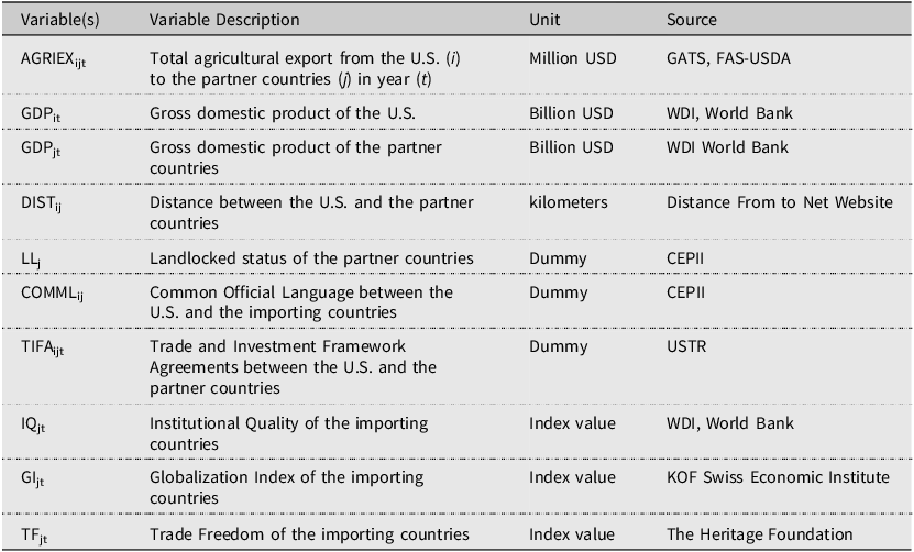
The exporting and importing countries’ GDPs are the measure of economic mass, and the respective countries’ GDP data are derived in constant 2015 USD from the World Bank’s World Development Indicators (WDI) portal. Bigger economies are assumed to trade more because they have larger consumption and production possibilities, as hypothesized in the standard gravity model of trade. Based on capital-to-capital proximity, countries’ geographical distance was approximated in kilometers using figures from the DistanceFromTo platform (https://www.distancefromto.net/). Dummy variables were used to capture other geographical and cultural features. Landlocked countries were assigned a value of 1 and 0 otherwise, which reflects additional logistical burdens faced by countries without direct access to seaports (Raballand, Reference Raballand2003). Similarly, using CEPII data, a common official language variable was considered for the purpose of determining if the partner nation shared the same official language as the United States which is English (Conte et al., Reference Conte, Cotterlaz and Mayer2022). Although the use of a common language lowers transaction costs, its impact may differ on the basis of regional particulars (Abdullahi et al., Reference Abdullahi, Huo, Zhang and Azeez2021). One of the important policy variables in our analysis is whether or not the United States and its partner countries have a Trade and Investment Framework Agreement (TIFA). TIFAs are typically informal arrangements and implemented to promote cooperation and communication on trade and investment-related matters. The timing and signing information of TIFAs are available in the U.S. Representative Office of Trade (USTR) website. Empirical evidence suggests that these kinds of frameworks enhance trade efficiency by coordinating regulatory environments and cutting non-tariff barriers (Nguyen, Reference Nguyen2022; Zhu, Reference Zhu2023). By computing the average of six World Bank Worldwide Governance Indicators – control of corruption, voice and accountability, political stability, rule of law, government effectiveness, and regulatory quality – we considered Institutional Quality (IQ) as an independent variable for our study measuring governance-related determinants of trade (Kaufmann and Kraay, Reference Kaufmann and Kraay2024). Institutions are closely connected with trade flows in a way that they reduce uncertainty and improve enforcement, according to prior studies (Hou et al., Reference Hou, Wang and Xue2021; Scoppola and Raimondi, Reference Raimondi and Scoppola2025). The Globalization Index (GI) is a measure from the KOF Swiss Economic Institute that captures a nation’s integration into international systems economically, socially, and politically. This index offers a complete picture of a nation’s international interdependence taking into consideration the de jure (policy and regulatory openness) and de facto (actual trade and capital flows) dimensions (Dreher et al., Reference Dreher, Gaston and Martens2008; Potrafke, Reference Potrafke2014). Lastly, trade freedom (TF) has been traditionally viewed as a promoter of trade, but its actual effects can be country- and sector-specific, especially agriculture (Kimura and Lee, Reference Kimura and Lee2008; Dang, Reference Dang2024). TF integrates qualitative evaluation of non-tariff barriers, such as import quotas, licensing requirements, and regulatory obligations, with weighted average tariff rates. In this study, we sourced the TF data from the Heritage Foundation. Overall, our panel dataset contained a few missing observations. There were missing values of our IQ variable across all partners for the year 2001, and the measures of Angola’s trade freedom were missing from 2001 to 2005. These missing values were filled with linear interpolation to have an equal balance for estimation because these variables are composite annual indexes with smooth year-to-year changes (Gygli et al., Reference Gygli, Haelg, Potrafke and Sturm2019; Borchert et al., Reference Borchert, Larch, Shikher and Yotov2024). Table 1 provides an overview of the variables with their respective data sources.
Data description

Table 1 Long description
A table with 10 rows and 4 columns. The columns are labeled Variable(s), Variable Description, Unit, and Source. The rows are as follows: Row 1: AGRIEXijt, Total agricultural export from the U.S. (i) to the partner countries (j) in year (t), Million USD, GATS, FAS-USDA. Row 2: GDPit, Gross domestic product of the U.S., Billion USD, WDI, World Bank. Row 3: GDPjt, Gross domestic product of the partner countries, Billion USD, WDI World Bank. Row 4: DISTij, Distance between the U.S. and the partner countries, kilometers, Distance From to Net Website. Row 5: LLj, Landlocked status of the partner countries, Dummy, CEPII. Row 6: COMMLij, Common Official Language between the U.S. and the importing countries, Dummy, CEPII. Row 7: TIFAijt, Trade and Investment Framework Agreements between the U.S. and the partner countries, Dummy, USTR. Row 8: IQjt, Institutional Quality of the importing countries, Index value, WDI, World Bank. Row 9: GIjt, Globalization Index of the importing countries, Index value, KOF Swiss Economic Institute. Row 10: TFjt, Trade Freedom of the importing countries, Index value, The Heritage Foundation.
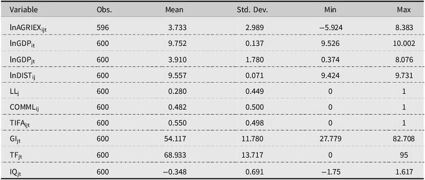
Table 2 contains the summary statistics of the variables, and these statistics reveal that U.S. agricultural exports to 25 countries in South Asia, Southeast Asia, and Southern Africa are highly heterogeneous, with a log mean of 3.733 and a large standard deviation of 2.989. The importing countries’ economic scale (ln GDP j mean = 3.910), globalization level (GI j mean = 54.117), and institutional level (IQ j mean = −0.348) differ significantly, which reflects the diversity of trade between partners. From among the sample countries, about 28% are landlocked, and 48% have the same official language as the United States.
Summary statistics

Table 2 Long description
The table presents summary statistics for several variables. It includes 11 rows and 6 columns. The columns are labeled Variable, Obs., Mean, Std. Dev., Min, and Max. The variables listed are lnAGRIEX_ijt, lnGDP_it, lnGDP_pt, lnDIST_ij, LL_i, COMML_ij, TIFA_ijt, GI_ijt, TF_ijt, and IQ_ijt. Each row provides the observation count, mean, standard deviation, minimum, and maximum values for each variable. For example, lnAGRIEX_ijt has 596 observations, a mean of 3.733, a standard deviation of 2.989, a minimum of -5.924, and a maximum of 8.383. The table captures the heterogeneity and diversity in the data related to U.S. agricultural exports to various countries.
The correlation matrix of our study variables is presented in Table A.1 (see Appendix A), which demonstrates that the GDP of the United States and the importing countries are strongly positively correlated with U.S. agricultural exports (r = 0.862). This correlation implies that the economic size of partners is one of the primary determinants of trade flows. Furthermore, high positive correlations exist between exports and TIFA agreement (r = 0.668) and globalization (r = 0.518). Conversely, trade is negatively related to distance, landlockedness, and lack of a common language which supports the geography- and culture-based hurdles. In general, the evidence is confirmatory evidence of significant trade-related and institution-related factors’ impact on U.S. agricultural exports, demonstrating empirical utility of the extensions to gravity models.
4. Results and discussion
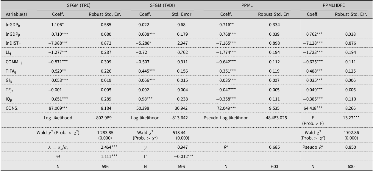
Table 3 presents the results of the estimations of the Greene’s (Reference Greene2005) True Random Effects Stochastic Frontier Gravity Model (SFGM (TRE), Battese and Coelli’s (Reference Battese and Coelli1992) Time-Varying Decay Inefficiency Stochastic Frontier Gravity Model (SFGM (TVDI), Poisson Pseudo Maximum Likelihood (PPML), and Poisson Pseudo Maximum Likelihood with high dimensional fixed effect (PPMLHDFE). Meanwhile, we presented the result of Fixed Effects (FE) and Random Effects (RE) with robust standard errors in Table B.1 (please see Appendix B). We considered SFGM (TRE) as the primary model in our study because it is an appropriate model that accounts for the unobserved and time-invariant heterogeneity across countries in the context of U.S. agricultural exports. With a significant inefficiency ratio (λ = 2.464***), the model is highly robust and finds inefficiency to be a main source of divergence from the expected trade frontier. A large log-likelihood value (−802.989) and Wald chi-square statistic (χ2 = 1,283.85, p < 0.001) also validate its goodness of fit. The SFGM (TVDI) model estimation allows inefficiency to change with time as a robustness check. The negative parameter of decay (η = −0.012***), i.e., trade inefficiency decreases with time, is consistent with possible policy reform, institutional development, or learning effects. Additionally, the inefficiency variance ratio (γ = 0.947) shows that the greater part of the residual variation from the model is due to inefficiency. The SFGM (TVDI) model yields a comparatively higher log-likelihood (–813.642) and it is theoretically and statistically consistent with the robustness of the primary conclusions drawn from the SFGM (TRE) formulation.
The estimated results of the determinants of U.S. Agricultural export with south asian, southeast asian and southern African countries

Table 3 Long description
The table presents the estimated results of various models analyzing the determinants of U.S. agricultural exports with South Asian, Southeast Asian, and Southern African countries. It includes four models: SFGM (TRE), SFGM (TVDI), PPML, and PPMLHDFE. The table has 18 rows and 12 columns. Column headers are Variable(s), SFGM (TRE) Coeff., SFGM (TRE) Robust Std. Err., SFGM (TVDI) Coeff., SFGM (TVDI) Std. Error, PPML Coeff., PPML Robust Std. Err., PPMLHDFE Coeff., PPMLHDFE Robust Std. Err., Log-likelihood, Wald chi-square (Prob. > chi-square), lambda, theta, and N. Row labels include variables such as lnGDP_ij, lnGDP_it, lnDIST_ij, LL_j, COMML_ij, TIFA_ij, GI_jt, TF_ij, IQ_jt, and CONS. Each row provides the coefficients and robust standard errors for each model. Notable trends include significant coefficients for variables like lnGDP_it, lnDIST_ij, and TIFA_ij across different models, indicating their importance in determining U.S. agricultural exports.
N.B. ***p < 0.01, **p < 0.05, *p < 0.1.
We found that exporter’s GDP (GDP i ) has a significant negative impact on U.S. agricultural exports for several specifications in our study, e.g., SFGM (TRE), PPML, FE, RE. This negative significant negative impact of GDP i on U.S. agricultural exports implies that higher U.S. GDP decreases U.S. agricultural exports to the partner countries. Even though the gravity model of trade traditionally posits that both the exporter’s GDP (GDP i ) and importers’ GDP (GDP j ) have a positive impact on bilateral trade flow (Atif et al., Reference Atif, Mahmood, Haiyun, Mao and Paniagua2019; Mulabdic and Yasar, Reference Mulabdic and Yasar2021; Ebaidalla and Ali, Reference Ebaidalla and Ali2022), but negative effect can occur. For example, Bojnec and Fertő (Reference Bojnec and Fertő2009) examined agro-food trade among 29 OECD countries and found that exporter GDP generally exerted a negative or insignificant effect on agricultural and food exports, suggesting that larger and more diversified economies tended to orient production toward domestic or higher-value markets rather than volume-based agricultural exports. Similarly, Mosikari and Eita (Reference Mosikari and Eita2016) found a significantly negative exporter-GDP effect for South Africa’s agriculture, forestry, and fishing exports, arguing that higher GDP reflected increased self-sufficiency and reduced export orientation. Guan and Sheong (Reference Guan and Ip Ping Sheong2020) further showed that GDP negatively affected African exports to China while positively influencing imports, indicating that rising domestic income could reduce export dependence in specific regional trade relationships. Therefore, this counterintuitive result can be due to structural forces that the standard gravity variables fail to account for. Heerman and Sheldon (Reference Heerman and Sheldon2018) noted that agro-ecological determinants such as climate, altitude, and land availability are more reliable predictors of agricultural trade flows than the exporter’s GDP in the systematic heterogeneity (SH) gravity model. Additionally, despite the enormity, affluent nations such as the United States tend to underperform in productivity-adjusted farm exports because of capital and environmental constraints (Heerman and Sheldon, Reference Heerman and Sheldon2018). Coinciding with this, Morrow (Reference Morrow2010) emphasized the importance of resource endowments in the sector and productivity levels, adding that GDP is not always the best indicator of export performance. In the United States, capital-intensive and service sectors have been the main drivers of sustained GDP growth.
This could potentially lessen agricultural export orientation through resource reallocation and increased domestic demand. The validity of our findings is supported by Brondino’s (Reference Brondino2021) observation that globalization and capital mobility may have weakened conventional frameworks of comparative advantage for developed economies.
Our empirical findings demonstrate that importers’ GDP (GDP j remains positively significant across all models except FE, which aligns with theoretical expectations and prior studies (Fadeyi et al., Reference Fadeyi, Bahta, Ogundeji and Willemse2014; Karemera et al., Reference Karemera, Koo, Smalls and Whiteside2015; Irshad et al., Reference Irshad, Xin, Hui and Arshad2018). For instance, the SFGM (TRE) model suggests that a 1% increase in importers’ GDP is associated with a 0.710% increase in U.S. agricultural exports, ceteris paribus. Income growth drives up agricultural import volumes, and the growing demand for imported food commodities in emerging markets, especially in South Asia, ASEAN, and Southern Africa, is reflected in this significant correlation. Even though GDP i appears to be a context-dependent and structurally constrained variable, GDP j remains a consistent and significant determinant of U.S. agricultural export performance.
Distance serves as a proxy for transport costs and also for various intangible barriers such as cultural and informational distances, which might have an impact on trade flows. Disdier and Head (Reference Disdier and Head2008) confirmed that geographical distance remains a substantial barrier to international trade despite globalization and technological developments. Our empirical findings suggest that geographic distance between the United States and its trading partners in South Asia, ASEAN, and Southern Africa exerts a significant negative influence on U.S. agricultural exports. Specifically, the negative impact of distance is more pronounced as our SFGM (TRE) results imply that a 1% increase in distance is associated with an 7.988% decrease in U.S. agricultural exports to the targeted markets, holding other factors constant. The large coefficient of lnDistance is also supported by the other models’ results, such as SFGM(TVDI), PPML, and PPMLHDFE. This is consistent with longstanding evidence in the gravity trade literature that distance acts as a key trade friction by raising transport costs, increasing delivery times, and introducing logistical uncertainty. Similar conclusions have also been made by Shuai (Reference Shuai2010), Atif et al. (Reference Atif, Liu and Mahmood2016), Lateef et al., (Reference Lateef, Tong and Riaz2018), and Cevik (Reference Cevik2023), who support the finding that trade is facilitated by proximity and hindered by remoteness.
Landlocked nations suffer extra trade barriers due to higher transportation and transit costs, dependency on neighboring countries’ infrastructure, and potential political and administrative impediments. In gravity model applications, the compounding problem of landlockedness (LL) is also well-established. In our results, landlockedness is found to be significantly negative across the SFGM (TRE), PPML, and PPMLHDFE and RE models. In our preferred SFGM (TRE) model, the coefficient −1.277 implies that U.S. agricultural exports to landlocked importing countries are approximately (e −1.277−1) × 100 ∼ 72% lower than those to coastal countries. This finding reflects substantial structural trade-cost disadvantages associated with the absence of direct access to seaports. Importantly, this effect operates through the trade frontier itself and is distinct from trade inefficiency captured by the stochastic frontier component. Raballand (Reference Raballand2003) analyzed 46 countries’ data (18 of which are landlocked) and found that being landlocked reduces trade by more than 80%. Four alternative metrics are used in his study to measure landlockedness: the number of borders with coastal countries, the number of national borders that must be crossed, the shortest distance to the closest major port, and the existence of a landlocked dummy. All four metrics showed that landlocked nations had substantially higher transportation costs, mostly as a result of inefficient border crossings and restrictions on overland travel. The high cost of trade in inland economies is also influenced by the number of borders that must be crossed, which serves as a stand-in for logistical and bureaucratic friction. Landlocked nations are especially vulnerable to border crossing delays. Djankov et al., (Reference Djankov, Freund and Pham2010) found that each additional day lowered exports by 4% in the case of landlocked countries, and this illustrates how geographic isolation impedes trade.
Our empirical results suggest that the common official language between the United States and its partner countries negatively influences U.S. agricultural exports, which contradicts the standard conjecture that similarity in language facilitates trade by diminishing information barriers and transaction costs. Common language and colonial linkages are frequently used in gravity models as proxies for cultural and historical proximity, and these “non-traditional” determinants of economic exchange have been shown to be important factors shaping trade patterns (Head and Mayer, Reference Head and Mayer2014). Rauch (Reference Rauch1999) similarly argues that cultural and language similarities, as well as contiguity, should be incorporated into gravity models because trade – particularly in differentiated goods – often relies on networks rather than anonymous markets. However, this counterintuitive result may happen if the U.S. agricultural exports became more responsive to demand-side factors such as food security, local tastes, and market size compared to cultural or linguistic compatibility. This interpretation is consistent with Hutchinson (Reference Hutchinson2002), who finds that both English as a first language and English as a second language are less important for exports than for imports, suggesting that language facilitates market access asymmetrically and does not uniformly benefit exporters. Additionally, technological developments such as digital translation tools and the globalization of agricultural trade may be diminishing the importance of a common language by reducing information and transaction costs even in linguistically dissimilar markets. Other studies also support this context-specific finding. Atif et al., (Reference Atif, Liu and Mahmood2016) found no significant impact of a common language on Pakistan’s agri-food exports, while Khan et al. (Reference Khan, Chen and Lv2024) and Abdullahi et al., (Reference Abdullahi, Huo, Zhang and Azeez2021) revealed statistically significant negative effects of a common language on Pakistan’s vegetable exports and Nigeria’s agri-food trade, respectively. These findings are consistent with the broader conclusion in the gravity literature that the role of language in trade is not universal but varies across contexts and may be overshadowed by structural factors such as institutional ties and international integration.
The results of our stochastic frontier gravity model estimation reveal that belonging to a TIFA with the United States is positively and significantly associated with U.S. agricultural export performance with South Asian, ASEAN, and Southern African countries. This result is in line with more universal empirical findings setting out that trade agreements can reduce barriers to trade and make exporting more efficient (Masood et al., Reference Masood, Khurshid, Haider, Khurshid and Khokhar2022). Zhu (Reference Zhu2023) also proves that RTAs in East Asia, specifically involving big economies such as China, India, and Japan, yield significant gains in trade efficiency even when there are heterogeneous regional environments. Therefore, TIFAs can similarly improve U.S. export efficiency by focusing on the reduction of non-tariff barriers and deepening regulatory cooperation. From a policy standpoint, TIFAs offer organized forums for dialogue, harmonization of regulations, and facilitation of trade. Established in 2006, the U.S.–ASEAN TIFA supports programs such as the Expanded Economic Engagement (E3) Program and facilitates senior-level discussions through a Joint Council. Its goals include supply chain resilience, standards, SME development, and customs cooperation (ASEAN, 2020). In 2014, the United States exported more than $11 billion worth of agricultural commodities to ASEAN alone, demonstrating its impact at the sectoral level (The White House, 2015). Similar to this, TIFA agreements with South Africa, ECOWAS, and COMESA (USTR, 2025) provided institutional arrangements for enhancing trade, investment, and regulatory ties and facilitated the United States’ access to these promising markets. Therefore, TIFAs play a significant role in improving agricultural export efficiency, especially in non-FTA contexts where regulatory and institutional trade barriers persist.
Our findings indicate that globalization positively affects U.S. agricultural exports, supporting the overall empirical evidence that international economic integration stimulates trade flows. Analyzing the data of 265 countries and 170 industries, Borchert et al. (Reference Borchert, Larch, Shikher and Yotov2024) showed that globalization has increased bilateral trade by approximately 570%, even accounting for WTO and EU membership. By examining a gravity data set of over 4.6 million bilateral observations, Cevik (Reference Cevik2023) confirmed that trade openness, which is commonly used as a proxy for globalization, significantly increases trade even in post-pandemic periods. The resilience of globalization is further supported by Franco-Bedoya (Reference Franco-Bedoya2023), who suggests that there was no systematic retreat from globalization during international crises and geopolitical upheavals. The structural adaptability of globalization is further understood when the U.S.-China trade recovered from $557.1 billion in 2020 to $690.3 billion in 2022 despite supply chain changes and diplomatic tensions (Alfaro and Chor, Reference Alfaro and Chor2023). While the economic benefits of globalization are firmly established, Irwin (Reference Irwin2020) and Bowen et al., (Reference Bowen, Broz and Rosendorff2023) pointed out that its long-term sustainability depends on domestic policy activism, particularly on redistributive policies and social protection for those countries that are adversely affected by international competition. In the absence of such protection, political resistance to globalization can grow stronger, which can ultimately counter future possibilities for liberalization of trade.
We find that trade freedom is not significant in its effect on U.S. agricultural exports based on the results from our SFGM (TRE), SFGM (TVDI), FE, and RE models. However, trade freedom is found to be significantly positive in the PPML and PPMLHDFE models, indicating some model-specific sensitivity. These findings are in agreement with other empirical results refuting the persistent ability of trade freedom indicators to explain trade performance, particularly for the agricultural sector. Deluna and Cruz (Reference Deluna and Cruz2013). found that labor freedom and corruption freedom among economic freedom parameters only played a significant role in influencing trade efficiency in the Philippines’ merchandise exports. In wider terms, Kimura and Lee (Reference Kimura and Lee2008) compared bilateral services trade between 28 countries over the period 1992–2003 using the Heritage Foundation Index and the Fraser Institute’s Economic Freedom of the World Index. Their research revealed that whereas economies with more economic freedom had more services traded, the factor “freedom to trade internationally” did not matter at all. The superior determinants of trade performance were instead found in regulatory factors such as the size of government, freedom in business, and credit market regulation.
The results of the primary model of our study (SGFM (TRE)) suggests that higher U.S. agricultural exports to South Asian, Southeast Asian, and Southern African countries are associated with better institutional quality in these regions. This supports the idea that strong institutions, such as the rule of law, anti-corruption, regulation effectiveness, and government stability, promote trade by lowering transaction costs, uncertainty, and the risk of contract enforcement. In fact, weak institutions can deter trade by causing inefficiencies comparable to formal barriers, which implies that institutional quality can have an impact on bilateral trade just as strongly as it can on the removal of tariffs (De Groot et al., Reference De Groot, Linders, Rietveld and Subramanian2004; De Groot et al., Reference De Groot, Linders and Rietveld2005). While Francois and Manchin (Reference Francois and Manchin2013) argued that institutional vulnerabilities can result in protectionist trade restrictions, Capasso (Reference Capasso2004) revealed that high-quality institutions optimize resource utilization and minimize economic waste in an economy. Additionally, institutional quality lowers trade friction, mitigates default risk, and fosters a stable business environment (Wu et al., Reference Wu, Li and Samsell2012, Chowdhury & Audretsch, Reference Chowdhury and Audretsch2014; Yu et al., Reference Yu, Beugelsdijk and De Haan2014). Thus, institutional quality plays a crucial role in facilitating agricultural trade, particularly in areas where governance frameworks affect the effectiveness and dependability of cross-border transactions.
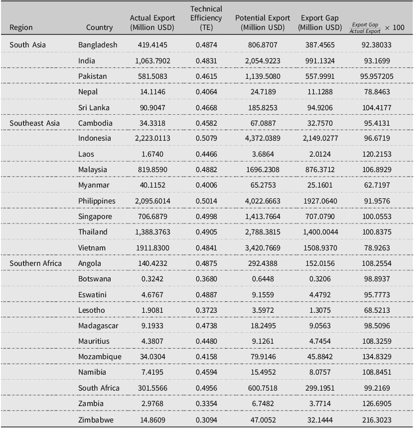
Table 4 presents the average TE estimates, actual exports, potential exports, and the export gap of U.S. agricultural trade with selected countries in South Asia, Southeast Asia, and Southern Africa. TE is derived from the stochastic frontier gravity model (SFGM (TRE)), and it measures how efficiently the United States is able to convert its agricultural export potential into actual trade, given partner-country characteristics such as GDP, distance, landlockedness, institutional quality, and globalization. The results indicate a wide variance in efficiency levels and export gaps across the regions and countries assessed. Technical efficiency scores in South Asia range from 0.4064 (Nepal) to 0.4874 (Bangladesh). With an estimated potential of $2.05 billion, the United States exported $1.06 billion to India, leaving a $991 million export gap (TE = 0.4831). Similarly, Pakistan records $581 million in actual exports with a potential of $1.13 billion (TE = 0.4615), while Bangladesh records $419 million in actual exports against a potential of $806 million. The United States exhibits efficiency losses even in smaller markets like Nepal and Sri Lanka; for example, it exports $14.114 million to Nepal when its potential export level is $24.71 million. These disparities show that the United States has consistently performed poorly in this region despite having clear market demand. Therefore, it also makes an indication that the lower TE scores of the United States in this region may have been caused by structural and institutional constraints.
Average technical efficiency, potential, and gap of U.S. Agricultural export to south asian, southeast asian, and southern African countries

In Southeast Asia, TE scores are marginally higher, ranging from 0.4006 in Myanmar to 0.5079 in Indonesia, yet the region still exhibits large absolute export gaps. Indonesia received the highest U.S. agricultural export in the region – $2.22 billion, with a potential export value of $4.37 billion, reflecting a gap of approximately $2.14 billion. The Philippines follows with actual exports of $2.09 billion and a potential of $4.02 billion (TE = 0.5014). Countries such as Malaysia, Vietnam, Thailand, and Singapore all exhibit export gaps ranging from $707 million to $1.50 billion despite having relatively better infrastructure and trade integration, while lower-volume markets like Laos and Cambodia show smaller absolute gaps but similar efficiency ratios. These findings suggest that efficiency constraints persist even in economies that are open and economically integrated.
Although South Africa’s technical efficiency exceeds that of India, the Southern African region as a whole exhibits lower efficiency due to the relatively poor performance of several other countries in the region. For example, Zambia and Zimbabwe have the highest relative inefficiencies in this category with average TE scores of 0.3354 and 0.3094, respectively. South Africa is the largest trading partner of the United States in Southern Africa. The United States exported roughly $302 million in agricultural products to South Africa, with a potential of $600 million (TE = 0.4956), leaving more than $300 million as an export gap. Other countries in the region, such as Angola, Mozambique, and Namibia, show varying degrees of underperformance, with export gaps ranging from $8 million to $153 million.
We calculate unrealized export potential relative to current trade using the relative export gap, defined as (Export Gap / Actual Export) × 100. This measure highlights countries where U.S. agricultural exports are underperforming relative to their estimated potential. Some markets exhibit very large relative export gaps, such as Zimbabwe (216.3%), Mozambique (134.8%), and Zambia (126.7%) indicating substantial inefficiencies. However, their strategic importance is limited because current U.S. agricultural exports to these countries are very small in absolute terms. In contrast, several large markets exhibit slightly lower relative gaps but substantially higher unrealized export values in dollar terms. For example, Indonesia shows a relative export gap of 96.7% with an unrealized export potential of approximately $2.15 billion, while India (93.2%), the Philippines (92.0%), Thailand (100%), Vietnam (78.9%) each represent unrealized export opportunities exceeding $1.4 billion. Therefore, these countries represent high-impact markets where U.S. could yield substantial gains in its agricultural exports by making modest improvements in export efficiency.
Overall, our results clearly indicate that across all three regions, U.S. agricultural exports fall substantially short of potential, not due to demand limitations, but due to inefficiencies arising from structural and institutional barriers. The model confirms that greater distance, landlockedness, and poor institutional quality are associated with lower TE, while higher levels of globalization, integration through trade agreements, and institutional development correspond with improved export efficiency. Hence, the findings of our study underscore that improving U.S. agricultural export performance in these emerging regions depends not only on identifying potential markets but on understanding and addressing the deeper inefficiencies that hinder trade facilitation and realization.
5. Limitations and future research
This study is subject to several limitations that also suggest promising avenues for future research. First, the analysis employs a stochastic frontier gravity model to benchmark U.S. agricultural export performance and estimate export efficiency and export gaps. While this framework is well-suited for assessing deviations from a maximum feasible trade frontier, it does not impose the general-equilibrium structure of structural gravity models that explicitly incorporate multilateral resistance terms and domestic trade flows. Future research could explore hybrid approaches that integrate structural gravity with stochastic frontier analysis to jointly assess general-equilibrium trade responses and export efficiency. Second, the empirical analysis focuses on aggregated U.S. agricultural exports. Although this aggregation allows for a comprehensive assessment of overall export performance, it limits the ability to construct intra-national (domestic) trade flows in a manner consistent with structural gravity requirements. Future studies using commodity-level data – where domestic production and sales can be more accurately matched with exports – could incorporate intra-national trade flows and examine how domestic demand interacts with export efficiency at a more disaggregated level. Third, while the stochastic frontier framework captures latent trade resistance through the inefficiency term, it does not explicitly disentangle specific sources of inefficiency such as infrastructure quality, logistics performance, or regulatory barriers. Future research could extend the model by incorporating inefficiency-effects specifications or external indicators to better identify the channels through which institutional and policy factors influence export performance. Finally, the present study focuses on a cross-country comparative analysis of under-explored markets. Future research could examine the dynamic evolution of export efficiency over time, assess the impact of specific trade agreements or policy shocks within a frontier framework, or compare frontier-based results with structural-gravity counterfactual simulations to provide complementary policy insights.
6. Conclusion and policy recommendations
This study examines the structural-institutional and economic drivers, unrealized potential, and the technical efficiency of the U.S. agricultural exports to 25 countries of South Asia, Southeast Asia, and Southern Africa from 2000 to 2022. Using a SFGM as the primary analytical model, we have established robust and statistically significant impacts of key economic and institutional factors. GDP of the importing countries is a positive and statistically significant contributor to U.S. agricultural export performance, reflecting income-driven demand in importing nations. The impact of the U.S. GDP is found to be statistically insignificant and negative, suggesting that reduced export orientation of the agricultural products can be linked with domestic growth through internal consumption or resource reallocation. Physical trade barriers have statistically significant negative effects, especially when it comes to geographic distance and the landlocked status of importing countries. The results lend support to the hypothesis that transport costs and market access constraints continue to be important obstructions to optimal export performance. On the contrary, our results reveal that participation in Trade and Investment Framework Agreements (TIFAs), globalization, and improved institutional quality positively impact U.S. agricultural exports. Interestingly, trade freedom does not emerge as a statistically significant factor in our results, which suggests that broader structural and institutional determinants may hold greater explanatory power in agricultural trade outcomes.
The technical inefficiency of US agricultural product exports to partner nations ranges from 0.30 to 0.51, reflecting a notable discrepancy between potential and actual export volumes. India, Bangladesh, Pakistan, Indonesia, Vietnam, Thailand, Singapore, the Philippines, and South Africa have the largest export gaps, indicating billions of missed export dollars for the United States.
Based on the empirical insights from this study, we propose the following policy recommendations: First, the United States must prioritize strategic diversification of agricultural exports by engaging more intensely with underachieving but high-potential markets like those defined in this study. Reducing overreliance on a smaller number of countries, i.e., China, Mexico, and Canada, the United States can minimize its exposure to economic shocks and geopolitical instabilities as well as increase its long-term export resilience. Second, institutionalization and operationalization of TIFAs in those states with a history of regulatory inefficiencies, such as Zimbabwe, Bangladesh, Pakistan, and Mozambique, should be promoted. As TIFAs are flexible alternatives to complete free trade agreements and they can play a pivotal role in handling non-tariff trade barriers and driving regulatory convergence. Third, the United States can provide targeted infrastructure support to landlocked and logistically disadvantaged countries through bilateral development assistance, public–private investment schemes, and multilateral partnerships on trade facilitation and logistics reform. Investment in digital customs systems, trade corridors, and cross-border logistics facilities will also be needed to lower transaction costs and increase supply chain resilience, especially for perishable agricultural products. Fourth, improving institutional quality in countries with significant untapped potential for U.S. agricultural exports should be one of the key focus of U.S. trade policy. Supporting prospective importing countries in areas such as contract enforcement, food safety systems, regulatory transparency, and anti-corruption measures can help reduce trade-related risks, build trust, and improve export efficiency. Lastly, given the statistical insignificance of trade freedom in our study, U.S. trade policy needs to move away from its long-standing tariff-based paradigm. More than that, a new, broader framework is needed – one that fosters value chain integration, capacity building, and market access facilitation in partner countries, especially where non-tariff and logistics barriers hinder U.S. agricultural exports.
Supplementary material
The supplementary material for this article can be found at https://doi.org/10.1017/aae.2026.10041.
Data availability statement
The data that support the findings of this study are available on request.
Author contribution
Conceptualization, T.K.G., and D.H.; Data Curation, T.K.G.; Formal Analysis, T.K.G.; Funding Acquisition, D.H.; Methodology, T.K.G., D.H., S.D.; Software, T.K.G.; Supervision, D.H., S.D.; Writing-Original Draft, T.K.G.; Writing - Review and Editing: T.K.G., D.H., S.D.
Financial support
This research was partially funded by a cooperative agreement with the Office of the Chief Economist-USDA and by the Combest Endowed Chair for Agricultural Competitiveness at Texas Tech University.
Competing interests
All authors declare none.
AI contributions to research
AI is used to correct grammar errors and sentence structures to improve the manuscript’s clarity and readability.


 Open access