


1. Introduction
Time preferences involving gains and losses are crucial in many decision -making processes. Researchers have extensively studied the discounting behaviors associated with time preferences in gain and loss domains, and findings suggest that these preferences differ. Individuals tend to discount future outcomes more heavily in gain domains compared with loss domains (e.g., Benzion et al., Reference Benzion, Rapoport and Yagil1989; Ikeda et al., Reference Ikeda, Kang and Ohtake2010; MacKeigan et al., Reference MacKeigan, Larson, Draugalis, Bootman and Burns1993; Molouki et al., Reference Molouki, Hardisty and Caruso2019; Thaler, Reference Thaler1981). This phenomenon is commonly referred to as the sign effect (Frederick et al., Reference Frederick, Loewenstein and O’Donoghue2002).
Intertemporal decision-making often entails trade-offs between gains and losses, which we can classify into two distinct domains in this article: the investment domain and the loan domain. The investment domain involves losses sooner and gains later. Such situations include instances where individuals forego immediate consumption of enjoyable goods or services to save money, with the expectation of receiving greater benefits in the future. This is commonly observed in contexts such as pension plans and investment portfolios. Conversely, the loan domain involves gains sooner and losses later. Such situations include instances where individuals make purchases using credit, enjoying immediate gains in the form of goods or services, but incurring future losses when they must repay the borrowed amount, as seen in contexts such as credit card debt and mortgages.
Despite the apparent importance of these domains, the difference in time preferences between them has not been thoroughly explored, except in a few studies (Ma et al., Reference Ma, Wang, Chen, He, Sun, Sun and Jiang2021; Meissner and Albrecht, Reference Meissner and Albrecht2022; Schleich et al., Reference Schleich, Faure and Meissner2021; Walters et al., Reference Walters, Erner, Fox, Scholten, Read and Trepel2016). These studies have shown that debts from loans are discounted at a lower rate than returns from investments, a phenomenon referred to as saving–borrowing asymmetry or debt aversion. Meissner and Albrecht (Reference Meissner and Albrecht2022) allowed participants to accept or reject various debt and saving contracts with an incentivized experiment. They consistently observed that participants systematically preferred saving contracts over debt contracts, even after controlling for time preferences, risk aversion, and loss aversion. Their structural estimation revealed that a substantial majority (89%) of participants exhibited aversion to being in debt. In a related line of work, Ma et al. (Reference Ma, Wang, Chen, He, Sun, Sun and Jiang2021) directly compared mixed intertemporal trade-offs (involving a loss now and a gain later, or vice versa) with pure gain and pure loss intertemporal choices. They found significant differences in discounting across these types of trade-offs: participants discounted most steeply in pure gain choices, followed by sooner-loss/later-gain (investment-type choices), then pure losses, and least steeply in sooner-gain/later-loss conditions (loan-type choices).
Given the substantial influence of domains on time preferences, it is reasonable to consider that the framing of intertemporal choices across different domains may also impact preferences. The framing effect is a well-established phenomenon in economics, psychology, and other disciplines (Tversky and Kahneman, Reference Tversky and Kahneman1981). This effect suggests that decisions are affected by how choices are presented, even when the final consequences of the options remain unchanged.
Loewenstein (Reference Loewenstein1988) highlighted that the way intertemporal options are presented as either speeding up or delaying outcomes influences choices significantly. For instance, individuals who anticipated receiving a Video Cassette Recorder in a year were willing to pay an average of $54 to get it right away, whereas those expecting it immediately required an average of $126 to agree to a one-year delay. Additionally, the strength of framing effects can even reverse the sign effect, showing that individuals are more inclined to discount future outcomes by merely changing the frames of the intertemporal choices decisions, for example, an acceleration frame in which the default is to realize the outcomes in the future and a delayed frame in which the default is to realize the outcomes today (Appelt et al., Reference Appelt, Hardisty and Weber2011; Benzion et al., Reference Benzion, Rapoport and Yagil1989; Shelley, Reference Shelley1993, Reference Shelley1994; Yamamoto et al., Reference Yamamoto, Shiba and Hanaki2020).
Framing choices as multiple events has been shown to have an impact on preferences, as demonstrated by Thaler (Reference Thaler1985) and Thaler and Johnson (Reference Thaler and Johnson1990). Thaler’s study involved framing outcomes as multiple events, and participants were asked to evaluate which frames they considered to be more favorable. For instance, they were presented with a choice between receiving $100 and then paying $80, or receiving $20 as a single outcome. The majority of participants strictly preferred the single outcome of receiving $20, despite the total outcomes being identical. Thaler and Johnson (Reference Thaler and Johnson1990) showed further evidence that separating outcomes has an impact on preferences. Participants perceived greater happiness when gains were temporally separated, indicating a preference for receiving multiple gains separately. Linville and Fischer (Reference Linville and Fischer1991) also found similar results, in which participants preferred to temporally separate two positive events.
This article specifically focuses on a type of framing similar to Thaler (Reference Thaler1985), which involves dividing outcomes into multiple components or manipulating the values of various outcomes to highlight common components in choices. In these situations, individuals tend to disregard shared components when making decisions. This phenomenon, known as cancellation, was demonstrated by Kahneman and Tversky (Reference Kahneman and Tversky1979). Participants in their study were presented with two choice options, each following a prior monetary bonus. In the first scenario, participants were given a bonus of $1,000 and subsequently had to choose between Lotteries A and B:
-
• Lottery A: a 50% chance of winning $1,000, with no win otherwise
-
• Lottery B: a guaranteed win of $500
In the second scenario, participants received a bonus of $2,000 and then had to choose between Lotteries C and D:
-
• Lottery C: a 50% chance of a loss of $1,000, with no loss otherwise
-
• Lottery D: a guaranteed loss of $500
Interestingly, despite equivalent overall outcomes between Lotteries A and C, as well as B and D, the majority favored Lottery B in the first scenario and Lottery C in the second. These results suggest that individuals tend to overlook the common prior bonus and instead focus on the specific outcomes of the lotteries.
Wu (Reference Wu1994) also observed the occurrence of cancellation in risky decision-making and revealed that participants tend to disregard outcomes that are transparently common in lottery choices. For instance, when given the choice between risky lotteries, X and Y:
-
• Lottery X: a 32% chance of winning $3,600, a 1% chance of winning $3,500, and no win otherwise
-
• Lottery Y: a 32% chance of winning $3,600, a 2% chance of winning $2,000, and no win otherwise
participants overlooked the shared chance of winning $3,600, focusing instead on the distinct outcomes to determine their preferred lottery.
Weber and Kirsner (Reference Weber and Kirsner1997) conducted a similar experiment investigating choices between a safer lottery and a riskier lottery. Each lottery consisted of three outcomes, with one outcome being common between both lotteries. By varying the magnitude of this common outcome, they found no significant impact on the selection of the riskier option, reinforcing the cancellation concept.
Cancellation has been documented in ambiguity choices as well (Schneider et al., Reference Schneider, Leland and Wilcox2018). The consistent observation of this phenomenon across different studies and variations in common outcome magnitudes attests to its durability in decision-making processes.
Given these findings, it is plausible to influence intertemporal decisions by manipulating common outcomes and framing intertemporal choices across various domains. This is due to individuals’ tendency to ignore common outcomes, which can lead to shifts in preferences depending on how options are structured. To our knowledge, no previous studies have demonstrated the impacts of Investment or Loan frames on decisions due to cancellation.
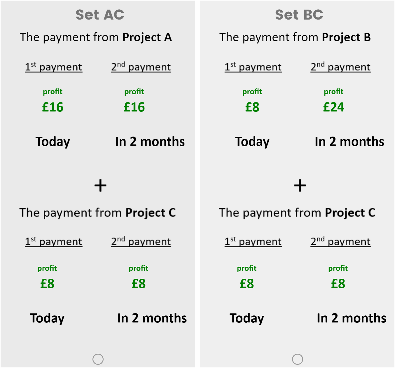
Our novel experiments presented binary intertemporal payment choices framed as investments and loans. Initially, we devised options that offered payments at both sooner and later dates, and then we divided the payments for each option into two components: common payments (CPs), where the payment amounts were common to both choices, and focal payments (FPs), where the payment amounts differed between choices. Consequently, each option has two distinct payments at both sooner and later dates (see Figure 1 for an example question). By varying the CP amounts, we can create different frames without altering total outcomes, effectively transforming the FPs into either investment or loan domains. This led us to hypothesize that CPs are disregarded and that decisions are based solely on FPs. Consequently, we predicted that time preferences would differ depending on whether the choice was presented in an Investment frame or a Loan frame, despite identical total outcomes—a clear deviation from normative decision-making.
The screenshot of the question (No frame, Net Gain section; Study 1).
Note: The payments from Project C in the question are common payments (CPs) because they are identical for both options. The remaining payments in the questions are focal payments (FPs).

2. Study overview
We conducted three online studies to test the hypothesis. Study 1 was designed to test our main hypothesis, examining how Investment and Loan frames affect time preferences . Study 2 investigated the boundary conditions of this framing effect by systematically manipulating the magnitude of the CPs, including significantly larger CPs—even those sufficient to change the total outcome’s domain—to test if these are disregarded by participants. Study 3 tested the robustness of our findings by introducing real financial incentives for the decision-making process.
Participants for all three studies (nationality: UK) were recruited via the online platform Prolific. The methods and analysis plans for each study were preregistered at aspredicted.org: Study 1 (#57211; https://aspredicted.org/9qgy-yhkd.pdf), Study 2 (#97463; https://aspredicted.org/vqzw-dggg.pdf), and Study 3 (#127343; https://aspredicted.org/xztv-6vnw.pdf).
2.1. Core choice structure
Across all studies, participants were presented with a series of binary intertemporal choices. In each trial, participants made intertemporal decisions by choosing between two project sets, referred to as Set AC and Set BC. Set AC consisted of Projects A and C, and Set BC consisted of Projects B and C. Both sets included Project C, which provided a payment common across the options—defined as the common payment (CP). Participants were explicitly told that all project sets were equally difficult and required the same amount of time to complete, ensuring that choices were based solely on payment structure.
Participants were told that projects could be either successful or unsuccessful, leading to profits (in the Net Gain section) or losses (in the Net Loss section). In each choice, participants were shown two payment bundles: one for today $({M}_0$
) and one for two months later (
$({M}_0$
) and one for two months later ( ${M}_2$
), denoted as
${M}_2$
), denoted as $\left({M}_0,{M}_2\right)$
. Positive values of M represent amounts received, while negative values indicate amounts lost. They were informed that the payments had already been determined and were asked to choose which set they preferred. The immediate payment that varied across the trials, using a modified Parameter Estimation by Sequential Testing (PEST) algorithm (Findlay, Reference Findlay1978; Walters et al., Reference Walters, Erner, Fox, Scholten, Read and Trepel2016), was different by study: in Studies 1 and 3, it was the payment for Set BC (i.e., Project B), while in Study 2, it was the payment for Set AC (i.e., Project A) (Findlay, Reference Findlay1978; Walters et al., Reference Walters, Erner, Fox, Scholten, Read and Trepel2016), as detailed below. This allowed us to identify the indifference point for each participant—that is, the value at which they were equally likely to choose Set AC or Set BC—thereby enabling calculation of their degree of impatience.
$\left({M}_0,{M}_2\right)$
. Positive values of M represent amounts received, while negative values indicate amounts lost. They were informed that the payments had already been determined and were asked to choose which set they preferred. The immediate payment that varied across the trials, using a modified Parameter Estimation by Sequential Testing (PEST) algorithm (Findlay, Reference Findlay1978; Walters et al., Reference Walters, Erner, Fox, Scholten, Read and Trepel2016), was different by study: in Studies 1 and 3, it was the payment for Set BC (i.e., Project B), while in Study 2, it was the payment for Set AC (i.e., Project A) (Findlay, Reference Findlay1978; Walters et al., Reference Walters, Erner, Fox, Scholten, Read and Trepel2016), as detailed below. This allowed us to identify the indifference point for each participant—that is, the value at which they were equally likely to choose Set AC or Set BC—thereby enabling calculation of their degree of impatience.
2.2. Preference elicitation and IDF calculation
To efficiently estimate each participant’s indifference point, we employed an elicitation method based on a modified version of the PEST algorithm (Findlay, Reference Findlay1978; Walters et al., Reference Walters, Erner, Fox, Scholten, Read and Trepel2016). This procedure adaptively adjusted the immediate payment value of one of the FPs (e.g., Project B’s ‘Today’ payment, denoted as X in Study 1) across multiple trials. The value of X was adjusted based on the following rules:
-
1. The value of X changed in response to participants’ previous choices: X decreased by the current step size when the participant chose the option containing X (i.e., Set BC in Study 1), and increased by the step size when they chose the option not containing X (i.e., Set AC in Study 1).
-
2. The initial step size was £4.
-
3. The step size was halved whenever the participant’s preference reversed across trials.
-
4. The step size remained constant otherwise.
-
5. The procedure terminated once the step size fell below £1.
This approach allowed for efficient estimation of preferences. From the resulting indifference point, we calculated each participant’s monthly individual discount factor (IDF), assuming an additive utility function and a standard linear model. For example , if the participant is indifferent between receiving £24 today and £24 in two months and receiving £20 today and £32 in two months ( $24+{\delta}^224=20+{\delta}^232$
), the resulting monthly IDF (
$24+{\delta}^224=20+{\delta}^232$
), the resulting monthly IDF ( $\delta$
) is approximately 0.71 given the assumptions above. Lower
$\delta$
) is approximately 0.71 given the assumptions above. Lower $\delta$
is interpreted as indicative of less patience.
$\delta$
is interpreted as indicative of less patience.
2.3. Debt aversion measure and demographic questions
After the intertemporal choice tasks, participants in all studies completed the Debt Aversion Measure (DAM) (Schleich et al., Reference Schleich, Faure and Meissner2021) consisting of seven questions on a 6-point scale to measure the level of debt aversion. The questions included, for example, ‘If I have debts, I like to pay them as soon as possible’ (1 = very much like me to 6 = not at all like me). We then created the variable DAM, describing the average score of the questions. This measure could potentially correlate with the variations in decisions between the Loan and Investment frames. Walters et al. (Reference Walters, Erner, Fox, Scholten, Read and Trepel2016) showed that individuals with higher levels of debt aversion, as measured by DAM, exhibited a more pronounced saving–borrowing asymmetry. At the end of the experiment, they answered the questions about their demographics, including age, gender, and education.
2.4. Exclusion criteria
As preregistered, we excluded two types of extreme responses from our analysis across all studies. First, we omitted observations that either weakly or strictly violated the principle of monotonicity, aligning with conventional methodologies for assessing individual preferences.
The other type of extreme case involved observations with extreme IDFs that fell outside the intended frames. This was necessary to ensure the integrity of the framing manipulation, as such extreme preferences would require altering the FPs into a different domain (e.g., turning a ‘No frame’ choice into an ‘Investment frame’ choice). Moreover, these preferences imply an extreme monthly IDF of more than 1.40, indicating that participants chose extremely patient options. Refer to Appendix B for a detailed explanation of these exclusion criteria.
The specific parameters, participant recruitment details, and unique design features for each study are presented in the sections that follow.
3. Study 1: Influence of Investment and Loan frames on intertemporal choices
Our first study was designed to test how Investment and Loan frames affect time preferences in Net Gain and Net Loss sections. In these scenarios, total outcomes are positive for the Net Gain section and negative for the Net Loss section. We will also confirm whether individuals ignore CPs when making these decisions.
3.1. Method
3.1.1. Participants
In Study 1, we recruited 300 participants for our experiment (39% female, mean age = 40 years, age range: 18–73 years). Our target was to collect approximately 100 participants each for three treatments: No frame, Investment frame, and Loan frame. The study took an average of 7 minutes and 18 seconds to complete (SD = 3 minutes and 40 seconds), and participants received a fixed compensation of £1.
3.1.2. Design and procedure
Participants were randomly assigned to one of three between-subjects framing conditions, each preserving identical total outcomes between the choice options. Each participant completed two sections: a Net Gain section and a Net Loss section, with the order randomized across participants.
3.1.3. CPs and FPs for each condition
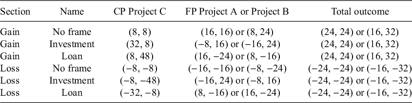
The parameters used in the first question for each frame are shown in Table 1 (see Figure 1 for an example question). In the No frame condition, the CPs were set to £8 today and £8 in two months, denoted as (8, 8). Participants chose between Set AC, which included FPs of (16, 16) plus the CPs (8, 8), and Set BC, which included FPs of (X, 24) plus the same CPs (8, 8). The value of X (ranging from £0.1 to £16) began at £8 and was adjusted based on participants’ previous choices, following the modified PEST procedure to identify the indifference point.
Parameters in the first questions for each treatment in Net Gain and Net Loss sections (Study 1)

Note: The payments in the experiments are denoted as $({M}_0,{M}_2$
), where
$({M}_0,{M}_2$
), where ${M}_0$
represents an immediate payment and
${M}_0$
represents an immediate payment and ${M}_2$
signifies a payment realized in 2 months. After the first question, the sooner payment of Project B is varied for each question based on the previous answers while the other payments remain fixed to identify their indifference points.
${M}_2$
signifies a payment realized in 2 months. After the first question, the sooner payment of Project B is varied for each question based on the previous answers while the other payments remain fixed to identify their indifference points.
In the Investment frame, the total outcomes were identical to those in the No frame, but the CPs were manipulated to (32, 8) to reflect an investment context. This resulted in the FPs being negative today and positive in two months (Set AC: (−8, 16); Set BC: (−16, 24) in the first question). In the Loan frame, the CPs were set to (8, 48), aligning the FPs with a loan context—positive today and negative in two months (Set AC: (16, −24); Set BC: (8, −16) in the first question).
The Net Loss section was a mirror image of the Net Gain section, with all parameter signs reversed. For example, in the No frame for the Net Loss section, choices were between Set AC, with (−16, −16) plus the CPs (−8, −8), and Set BC, comprising (X, −24) plus the CPs (−8, −8). Note that the FPs in the Investment and Loan frames remained consistent between the Net Gain and Net Loss sections for comparability. The order of the section was randomized.
To ensure that the participants understood the scenario, they were required to pass a comprehension question about the instructions before making the intertemporal choices. Similar to most previous articles investigating time preferences involving losses (e.g., Abdellaoui et al., Reference Abdellaoui, Gutierrez and Kemel2018), we utilized hypothetical scenarios due to ethical and logistical concerns associated with participants experiencing financial losses at different times. The issue of incentivizing decisions is revisited in Study 3. Detailed experimental instructions are available in the Online Appendix.
3.2. Results and discussion
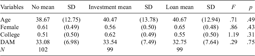
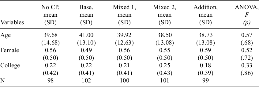
The demographic variables, including age, gender, and education, did not differ statistically across the treatments, indicating the randomization worked properly in this study (Table 2). We report our analyses in this section, excluding the observations by following the rules above .Footnote 1 However, we replicate the analyses including the observations that weakly violated monotonicity in Appendix B. The overall results do not change, indicating our results are robust.
The summary table of demographic variables (Study 1)

Note: The dummy variable College is assigned a value of 1 for subjects holding a college degree and 0 for those without. The variable DAM represents the total scores from the Debt Aversion Measure, which includes seven questions on a 6-point scale to assess the level of debt aversion.
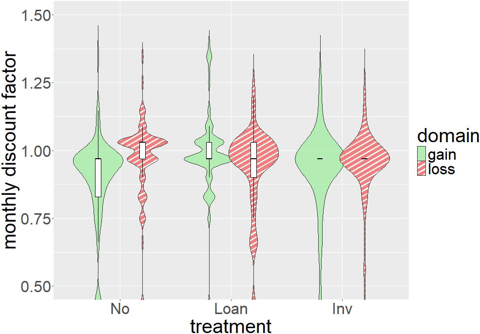
Figure 2 presents combined boxplots and violin plots of monthly IDF ( $\delta$
) for each treatment.Footnote
2
The IDFs are calculated from the indifference points derived using the elicitation method outlined in the preceding section.
$\delta$
) for each treatment.Footnote
2
The IDFs are calculated from the indifference points derived using the elicitation method outlined in the preceding section.
The monthly discount factors across treatments in net gain and net loss sections (Study 1).
Note: Each distribution combines a violin plot and a boxplot. Violin plots are filled solid green for gain and red-striped for loss. Boxplots are overlaid in white. The bold horizontal line in each box represents the median; the bottom and top edges of the box represent the first and third quartiles, respectively. The whiskers extend to the most extreme values within 1.5 times the interquartile range (IQR).

Figure 2 illustrates that IDFs appear to be lower in the No frame compared with the other frames in the Net Gain section, suggesting that framing affected the decisions. Due to the non-normal distribution of IDFs (Shapiro–Wilk test for each frame: p < .001), we employed nonparametric tests as they are more statistically appropriate in this case. We had not anticipated this highly skewed distribution of IDFs, which led us to deviate from our preregistered plan to use a parametric test for this study. The IDF in No frame significantly differed from that in the Investment frame (Mann–Whitney test; p = .02) and the Loan frame (p < .001). In the Net Loss section, the IDF appeared to be higher in the No frame than in the other domains in the graph, suggesting the framing effect in choices of losses as well. Indeed, the IDF in the No frame was different from that in the Investment frame (p < .01) and the Loan frame (p = .04). These findings support our hypothesis that framing influences time preferences in both sections.
In addition, the IDF in the Loan frame significantly differed from that in the Investment frame in the Net Gain section (Mann–Whitney test; p < .01), aligning with the concept of saving–borrowing asymmetry. However, the difference was not significant in the Net Loss section (p = .54).
Next, we compare the IDFs between the Net Gain and Net Loss sections. In the No frame, median IDFs were higher in the Net Loss section (Wilcoxon signed-rank test; p < .001), aligning with the sign effect. In contrast, in both the Investment and Loan frames, the IDFs were not significantly different (p = .07; p = .11). To further investigate these nonsignificant findings, equivalence testing was conducted using the two one-sided tests (TOST) procedure with equivalence bounds set at ±0.05. The TOST results confirmed that the IDFs for both treatments were statistically equivalent within these specified bounds (Investment frame: p < .001; Loan frame: p = .008). The nonsignificant and equivalence results in the two frames support the cancellation hypothesis: despite constant FPs, the varying CPs did not significantly affect decisions, indicating that participants focused on the FPs and disregarded the CPs in their decision-making process. In other words, regardless of the sets, participants were likely to consider choices as investments in the Investment frame and as loans in the Loan frame.
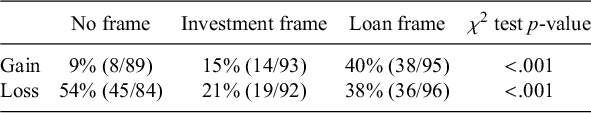
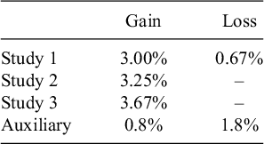
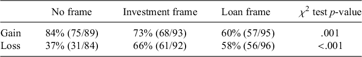
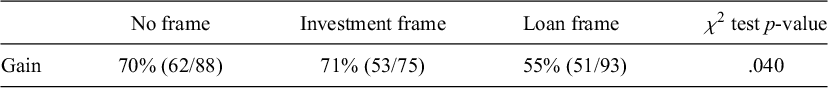
Interestingly, a non-negligible proportion of participants exhibited negative discounting—preferring to delay gains or to experience losses sooner. This phenomenon has also been documented in previous research, particularly in the context of losses (e.g., Hardisty and Weber, Reference Hardisty and Weber2009; Loewenstein, Reference Loewenstein1987; Loewenstein and Prelec, Reference Loewenstein and Prelec1991; Sun et al., Reference Sun, Ma, Zhou, Jiang and Li2022). Furthermore, the proportions appeared to differ substantially across conditions (Table 3). This pattern was analyzed in relation to treatment and section. Notably, the results from this analysis are consistent with those reported earlier, reinforcing our main findings.
Proportion of negative discounting in Study 1

In the Net Gain section, the proportion of participants showing negative discounting significantly differed across treatment conditions (χ2 test, p < .001). A similar pattern was observed in the Net Loss section (χ2 test, p < .001). Furthermore, in the No frame condition, a significantly higher proportion of participants exhibited negative discounting in the Net Loss section compared with the Net Gain section (McNemar test, p < .001). This finding is consistent with previous literature reporting increased negative discounting in loss contexts (e.g., Hardisty and Weber, Reference Hardisty and Weber2009; Yoon and Chapman, Reference Yoon and Chapman2016).
Additionally, debt aversion, as measured by the DAM,Footnote 3 was investigated by Walters et al. (Reference Walters, Erner, Fox, Scholten, Read and Trepel2016) and found to be more pronounced in individuals with higher levels of debt aversion. Our regression analysis, including only observations from the Investment and Loan frames in the Net Gain section, introduced a Loan dummy variable (1 for Loan frame, 0 otherwise). We excluded responses from the Net Loss section to maintain comparability with Walters et al. (Reference Walters, Erner, Fox, Scholten, Read and Trepel2016). The regression of IDFs against the DAM score, Loan, and their interaction term revealed that the interaction term was not significant, diverging from the findings of Walters et al. (Reference Walters, Erner, Fox, Scholten, Read and Trepel2016).
Nonetheless, the variation was not limited to the CPs; the total outcomes between the Net Gain and Net Loss sections also differed. Therefore, the influence of both CPs and total outcomes on decisions, potentially counterbalancing each other, could not be entirely ruled out. However, this scenario seems unlikely given the observed differences in IDFs between the No frame and the other frames in both sections, despite identical total outcomes.
4. Study 2: Investigating the boundary condition of CPs ignorance
We have thus far observed that time preferences are influenced by the Investment or Loan frames. This framing effect seems to arise from participants overlooking CPs between options.
Study 1 tested only one specific CP for each treatment in each section. Furthermore, the CPs were not large enough to change the domain of the total outcomes; total outcomes for all questions in the No, Investment, and Loan frames in the Net Gain section fell within the gain domain, and those in the Net Loss section were within the loss domain. Different values of CPs or total outcomes might significantly influence decisions. Higher values of CPs increase their relative importance, particularly if they are large enough to shift the domain of the total outcomes, making it less likely for CPs to be ignored.
In Study 2, we used various CPs for each treatment while keeping the FPs constant; thus, the total outcomes were no longer identical between main treatments. The highest absolute values of CPs in this study were £32 today and £76 in two months, higher than in Study 1, and some CPs were large enough to alter the domain of total outcomes.
To achieve this level of variation, a relatively large number of treatment conditions was required. To keep the design manageable while systematically manipulating CP size and direction, we focused only on the Net Gain section, where implementing a broad range of CP values was more feasible.
Therefore, the aim of this study is to explore the framing effect’s boundary conditions by manipulating CPs. The cancellation hypothesis posits that preferences should remain consistent as long as the FPs are identical. Conversely, if the domains of total outcomes or the magnitude of CPs influence decisions, we should observe variations in the degree of impatience in such scenarios.Footnote 4
4.1. Method
4.1.1. Participants
We recruited 800 participants for our experiment (48% female, mean age = 43 years, age range: 18–84 years). The study took an average of 6 minutes and 4 seconds to complete (SD = 3 minutes and 46 seconds), and participants received a fixed fee of £0.8.
4.1.2. Design and procedure
This study replicated the scenario from Study 1, but exclusively focused on the Net Gain section; consequently, there was no Net Loss section in this study. Participants were randomly assigned to one of eight treatments, with the initial parameters for each detailed in Table 4.
Parameters in the first questions for each treatment (Study 2)

Note: The payments in the experiments are denoted as $({M}_0,{M}_2$
), where
$({M}_0,{M}_2$
), where ${M}_0$
represents an immediate payment and
${M}_0$
represents an immediate payment and ${M}_2$
signifies a payment realized in 2 months. After the first question, the sooner payment of Project A is varied for each question based on the previous answers while the other payments remain fixed to identify their indifference points.
${M}_2$
signifies a payment realized in 2 months. After the first question, the sooner payment of Project A is varied for each question based on the previous answers while the other payments remain fixed to identify their indifference points.
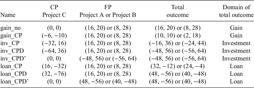
4.1.3. Six main treatments
Six main treatments featured identical FPs: (16, 20) for Project A and (8, 28) for Project B. The experiment encompassed three domains of total outcomes: gain, investment, and loan. Each domain within the main treatments had two distinct CPs. Specifically:
-
• In the gain domain, gain_no had no CP, whereas gain_CP included a CP of (−6, −10).
-
• In the investment domain, inv_CP presented a CP of (−32, 16), and inv_CPD offered a nearly doubled CP of (−64, 36).
-
• In the loan domain, loan_CP involved a CP of (16, −32), with loan_CPD providing a nearly doubled CP of (32, −76).
According to the cancellation hypothesis, the IDFs for all main treatments should be identical. However, should the domain of the total outcome exert an influence on decision-making, the IDFs across varying domains of total outcomes are expected to differ. For example, using gain_no as a baseline, the CP in loan_CP is sufficiently large to alter its domain from gain. Consequently, if the domain of the total outcome impacts decisions, differences in IDFs between these two conditions may be observed.
Furthermore, analyses within the same domain, such as inv_CP and inv_CPD, both of which fall under the investment domain, were conducted to assess whether larger CPs had a discernible effect on decision-making.
4.1.4. Two additional treatments
The remaining two domains were included to examine the effect of total outcomes. These treatments had no CPs; instead, their FPs were designed to match the total outcomes of the inv_CPD and loan_CPD conditions.
-
• The inv_CPD’ treatment presented FPs identical to the total outcomes of inv_CPD. Participants chose between Project A, starting at (−48, 56), and Project B, fixed at (−56, 64).
-
• Similarly, the loan_CPD’ treatment presented FPs identical to the total outcomes of loan_CPD. Participants chose between Project A, starting at (48, −56), and Project B, fixed at (40, −48).
4.2. Results and discussion
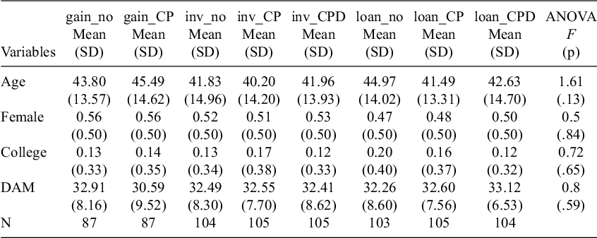
The demographic variables, including age, gender, and education, across the treatments were not statistically different, indicating the randomization worked properly in this study (Table 5). We applied the same exclusion criteria as in Study 1.Footnote 5
The summary table of demographic variables (Study 2)

Note: The dummy variable College is assigned a value of 1 for subjects holding a college degree and 0 for those without. The variable DAM represents the total scores from the Debt Aversion Measure, which includes seven questions on a 6-point scale to assess the level of debt aversion.
Figure 3 displays combined boxplots and violin plots of IDFs for each treatment, which aligns with the cancellation hypothesis. The IDFs of the six main treatments with different CPs did not show significant differences (Kruskal–Wallis test; p = .59). This outcome supports the cancellation hypothesis and suggests that participants primarily focused on the FPs while making their decisions, overlooking the CPs.
The monthly discount factors across treatments (Study 2).
Note: Each distribution consists of a violin plot and an overlaid boxplot. Treatments are grouped into gain (left), investment (middle), and loan (right) treatments. Violin plots are filled with no pattern for gains (black outline), yellow stripes for investment, and red circles for loan. The bold horizontal line inside each box represents the median; the bottom and top edges of the box indicate the first and third quartiles, respectively. Whiskers extend to the most extreme values within 1.5 times the interquartile range (IQR).

We further examined the possibility that preferences were influenced by both CPs and total outcomes, with these effects potentially neutralizing each other, although this is unlikely, as discussed in Study 1. To assess the impact of total outcomes, we analyzed two additional treatments.
The IDFs between loan_CPD and gain_no (treatments with identical FPs) were not significantly different (Mann–Whitney test; p = .56). To further investigate this nonsignificant finding, we conducted the TOST with equivalence bounds set at ±0.05 as in Study 1. The TOST results confirmed that the IDFs for these treatments were statistically equivalent within these specified bounds (p = .009). However, the IDFs between loan_CPD’ and gain_no (treatments with different FPs) differed significantly (p < .001).
Similarly, the IDFs between inv_CPD and gain_no (treatments with identical FPs) were not significantly different (Mann–Whitney test; p = .13). The TOST results almost confirmed that the IDFs for these treatments were statistically equivalent within the specified bounds, but the p-value was slightly higher than .05 (p = .056). However, substituting inv_CPD with inv_CPD’ and retesting these treatments showed that the IDFs between inv_CPD’ and gain_no (treatments with different FPs) were significantly different (p < .001). The findings further suggest participants’ primary focus on FPs rather than total outcomes.
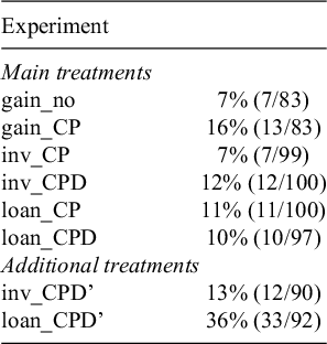
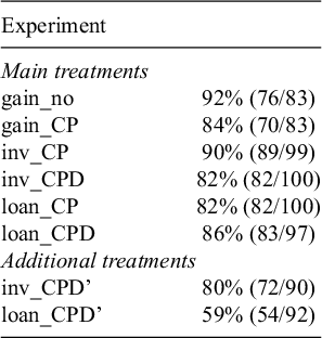
Consistent with the results from Study 1, a nonnegligible proportion of participants again exhibited negative discounting, preferring to delay gains or accelerate losses (Table 6). We repeated the same type of analysis as above, this time using the proportion of participants exhibiting negative discounting instead of IDFs. The results for treatments in which the total outcomes fell in the loan domain closely mirrored our earlier findings, providing additional support for our main conclusions.
Proportion of negative discounting in Study 2

Specifically, the comparison between loan_CPD and gain_no yielded a nonsignificant difference (χ2 test, p = .469), whereas the comparison between loan_CPD’ and gain_no showed a significant difference (p < .001). The difference between inv_CPD and gain_no was not significant (p = .281), and the difference between inv_CPD’ and gain_no was also not significant (p = .189).
In addition, the IDFs between inv_CPD’ and loan_CPD’ differed (p = .02). This is in line with the borrowing–saving asymmetry. We conducted a similar regression analysis to examine the relationship between the borrowing-saving asymmetry and DAM as in Study 1, but our findings again differed from the results of Walters et al. (Reference Walters, Erner, Fox, Scholten, Read and Trepel2016).Footnote 6
5. Study 3: Incentivizing choices in the net gain section
The aforementioned studies consistently demonstrate that framing exerts significant influence on individual time preferences. However, it is important to note that the decisions examined in these studies were not incentivized. While certain prior research articles have reported no disparity in discount factors between real and hypothetical rewards (Johnson and Bickel, Reference Johnson and Bickel2002; Madden et al., Reference Madden, Begotka, Raiff and Kastern2003), others have raised concerns regarding the hypothetical bias in intertemporal decisions. Frederick et al. (Reference Frederick, Loewenstein and O’Donoghue2002) argued that uncertainty exists regarding whether individuals, when presented with hypothetical rewards, are sufficiently motivated or capable of accurately predicting their actions if the outcomes were real. Furthermore, Kirby and Maraković (Reference Kirby and Maraković1995) discovered that individuals exhibited more impatience (i.e., higher IDFs) when the rewards were hypothetical.
To address this issue, we incorporated real incentives in the Net Gain section of Study 3 to test whether the framing effect persists under incentivized conditions. We chose to incentivize only the Net Gain section because it involved net positive outcomes. However, we decided not to incentivize the Net Loss section (as used in Study 1) due to several methodological and ethical challenges. Letting participants lose money in the future is ethically challenging since participants must be compensated after participating in experiments. To circumvent this issue, we could provide endowments or allow participants to earn some money to cover the losses by completing tasks. However, that procedure also presented significant flaws. If participants receive additional rewards not derived from the intertemporal questions, the rewards can be considered as another CP. Since we cannot differentiate these additional rewards from CPs in our analysis, we decided to incentivize only the Net Gain section (following the design of Study 1).
5.1. Method
5.1.1. Participants
We recruited 300 participants for our experiment (52% female, mean age = 44 years, age range: 18–81 years). The study took an average of 7 minutes and 26 seconds to complete (SD = 2 minutes and 58 seconds).
5.1.2. Design and procedure
This study mirrored the Net Gain section from Study 1, with the key distinction being the incentivization of intertemporal payment decisions. Participants were explicitly informed at the outset that there was a 1-in-10 chance of being selected for actual payment based on their choices in the experiment. They were also told that if selected, one of their intertemporal decisions would be randomly chosen, and they would receive the corresponding reward according to the payment timing specified in that question.
Additionally, we asked exploratory questions that were potentially correlated with intertemporal decisions according to the previous studies. These questions included household income and MacArthur Scale of Subjective Social Status (Adler et al., Reference Adler, Epel, Castellazzo and Ickovics2000).
For the participants selected for actual payment, the amounts were directly tied to the choices they made during the experiment, and they did not receive any show-up fee. One option was randomly selected for payment on its scheduled date, with immediate payments issued on the experiment day and deferred payments exactly two months from the experiment day. Those not selected for actual payment received a show-up fee of £0.8.
5.2. Results and discussion
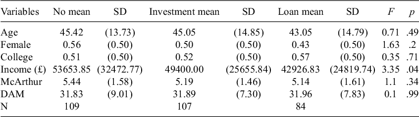
The demographic variables—including age, gender, education, income, and MacArthur Scale—showed no significant differences across treatments, with income being the sole exception. This outcome indicates that the randomization process was mostly effective, as evidenced by the consistency of the four variables (Table 7).Footnote 7
The summary table of demographic variables (Study 3)

Note: The dummy variable College is assigned a value of 1 for subjects holding a college degree and 0 for those without. The variable Income represents the annual gross income in GBP. The variable McArthur describes the average scores from the MacArthur Scale of Subjective Social Status. The variable DAM represents the total scores from the Debt Aversion Measure, which includes seven questions on a 6-point scale to assess the level of debt aversion.
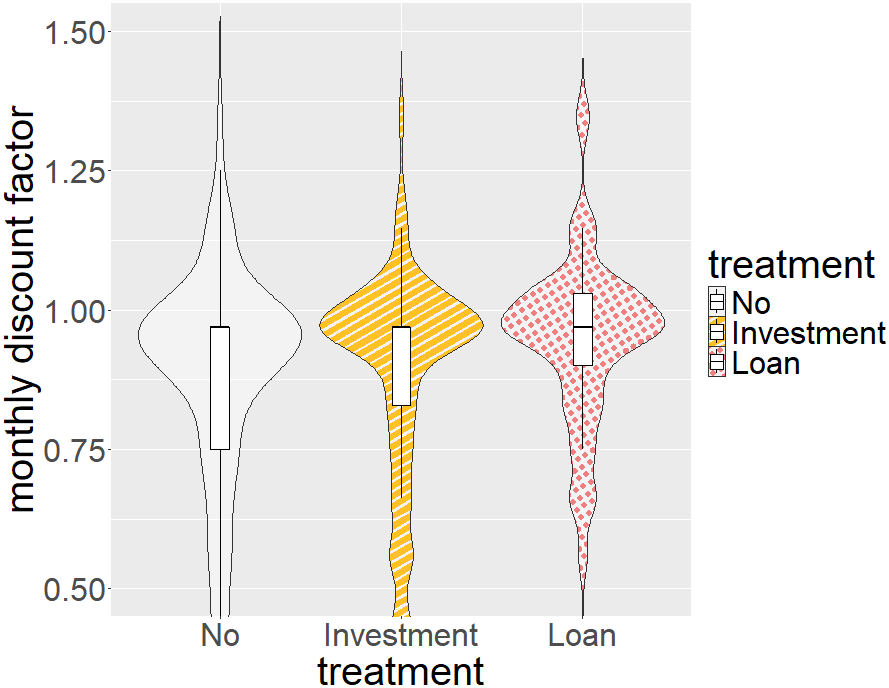
Figure 4 displays combined boxplots and violin plots of monthly IDFs for each treatment. Consistent with Study 1, we found significant differences between the Loan frame and No frame (Mann–Whitney test; p = .02). However, no significant difference was observed between the No frame and Investment frame (p = .37). In addition, the IDF in the Loan frame was not significantly different from that in the Investment frame (Mann–Whitney test; p = .13).
The monthly discount factors across the treatments (Study 3).
Note: Each treatment is represented by a violin plot and an overlaid boxplot. The No treatment is shown with no fill, the Investment treatment with yellow stripes, and the Loan treatment with red circles. The bold horizontal line inside each box represents the median; the bottom and top edges of the box indicate the first and third quartiles, respectively. Whiskers extend to values within 1.5 times the interquartile range (IQR) from the lower and upper quartiles.

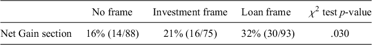
As in Studies 1 and 2, a non-negligible proportion of participants exhibited negative discounting—preferring to delay gains or to experience losses sooner—and this tendency varied considerably across conditions (Table 8). We repeated the analysis using the proportion of participants exhibiting negative discounting, rather than IDFs. The results were consistent with the analysis above, reinforcing our main conclusions.
Proportion of negative discounting in Study 3

The proportion of participants showing negative discounting significantly differed across treatment conditions (χ2 test, p = .030). To explore this further, we conducted pairwise chi-square tests. A significant difference was found between the No frame and Loan frame conditions (p = .01), while no significant difference was observed between the No frame and Investment frame (p = .373).
Repeating the regression analysis on the DAM from Study 1, our findings were consistent with those of Study 1 and did not reveal a stronger saving–borrowing asymmetry among individuals with higher scores on this measure.
We also analyzed the data based on participants’ income levels, categorizing observations by the median income level: those earning at or above the median were classified into the higher-income group, while those earning below the median were placed in the lower-income group. Notably, a significant impact of the Loan frame was observed among lower-income participants (Mann–Whitney test; p = .03), whereas this effect was absent among higher-income participants (p = .20).
We then compared these results with those from the Net Gain section in Study 1 to evaluate the impact of real financial incentives. The IDFs between the two studies were not statistically different in the No frame (Mann–Whitney test; p = .78) and Investment frame (p = .34), but the IDFs in the Loan frame were significantly different between the two studies (p = .04). Importantly, the core framing effect—the significant difference between the Loan frame and the No frame—was observed in both studies, enhancing the credibility of results from non-incentivized experiments.
6. General discussion
Our series of three studies investigated the impact of Investment and Loan frames on time preferences by manipulating CPs in intertemporal decisions. We demonstrated that this manipulation affects time preferences without changing the total payments.
This finding contrasts with standard economic theory, which posits that rational people should not change their time preferences as long as the total payments stay the same.
Beyond demonstrating this novel framing effect, our findings make a key theoretical contribution to the literature on decision heuristics by illuminating a key mechanism of the framing effect. Past research has studied framing effects in risky and ambiguous choices (Schneider et al., Reference Schneider, Leland and Wilcox2018; Weber and Kirsner, Reference Weber and Kirsner1997; Wu, Reference Wu1994). Our contribution is to show that the principle of cancellation is a powerful and surprisingly robust driver of behavior in intertemporal choice. By isolating FPs from CPs, we provide evidence that individuals do not integrate all components of an outcome stream. Instead, CP streams appear to be segregated and ignored, with decisions being disproportionately weighted toward the components that differ. Furthermore, this separation of payments into FPs and CPs represents our methodological contribution, providing a novel framework that could be applied to other types of choices, such as those involving both risk and time.
In summary, Study 1 showed that time preferences differed across the Investment, Loan, and No frame conditions, illustrating a significant framing effect. The pattern of choices suggests that participants focused mainly on the FPs and tended to disregard the CPs. Study 2 further examined the robustness and strength of the framing effect, demonstrating that large CPs—even those sufficient to change the domain of the total outcome—were generally disregarded. Study 3 introduced real financial incentives and confirmed the effect in the Loan frame, suggesting that the results of non-incentivized experiments were reliable.
In addition to analyzing IDFs, we also examined the proportion of participants exhibiting negative discounting—those who preferred to delay gains or accelerate losses. A non-negligible proportion of such participants was observed across all studies. Importantly, the pattern of results based on this measure closely mirrored those obtained using IDFs, further reinforcing the robustness and consistency of our findings. Specifically, in the Net Gain section, both the Investment and Loan frames showed a higher proportion of negative discounting compared with the No frame. This pattern suggests that these frames induced more patient behavior. This is consistent with debt aversion or saving–borrowing asymmetry (Meissner and Albrecht, Reference Meissner and Albrecht2022; Schleich et al., Reference Schleich, Faure and Meissner2021; Walters et al., Reference Walters, Erner, Fox, Scholten, Read and Trepel2016). It also aligns with findings that pure gain trade-offs exhibit stronger discounting than investment-type (loss–gain) or loan-type (gain–loss) intertemporal choices (Ma et al., Reference Ma, Wang, Chen, He, Sun, Sun and Jiang2021).
6.1. No effect of Investment frame in Study 3
The significant difference between the Loan frame and the No frame in the incentivized experiment provides strong evidence of a framing effect. In contrast, no difference in IDFs was observed between the No frame and Investment frame, which diverges from the findings of Study 1. The cause of this discrepancy is not immediately apparent, but it does not seem to be attributable to incentivization, as the IDFs in the No frame and Investment frame did not vary significantly between Studies 1 and 3, and the framing effect—the significant difference between the Loan frame and the No frame—was consistently observed in both studies.
6.2. Alternative hypothesis: The mixed-outcome effect
There might be an alternative explanation for the framing effect other than the cancellation hypothesis. In both the Investment and Loan frames, participants were presented with a mix of gains and losses—that is, some amounts to be received and some to be paid—at both the sooner and later dates. This differs from the No frame condition, in which options consisted exclusively of either all gains or all losses. To investigate whether exposure to mixed outcomes alone could influence decision-making, we conducted an auxiliary experiment (described in Appendix A). The results showed that the presence of both gains and losses in the same choice set did not significantly affect participants’ time preferences, suggesting that the framing effect cannot be attributed solely to the structure of mixed outcomes.
6.3. DAM and saving–borrowing asymmetry
The regression of IDFs against the DAM, a Loan dummy variable, and their interaction term revealed that the interaction term was not significant. Our results were different from the unpublished work of Walters et al. (Reference Walters, Erner, Fox, Scholten, Read and Trepel2016), who suggested that the borrowing–saving asymmetry is driven by individuals who are more averse to debt, as measured by the DAM. One potential explanation for this discrepancy is that the true relationship may be modest, and our experimental design—based on between-subjects comparisons with limited variation in framing conditions—may not have provided sufficient statistical power to detect the effect. In our studies, each participant was exposed to only one Investment condition and one Loan condition, and these were used in the statistical analysis to examine the relationship between borrowing–saving asymmetry and the DAM. Specifically, in Studies 1 and 3, we included only the Loan and Investment frames in the Net Gain section, and Study 2 focused exclusively on the Inv_CPD’ and Loan_CPD’ conditions. In contrast, Walters et al. employed a within-subjects design, where each participant completed multiple questions under both investment and loan framing conditions. This design likely provided greater statistical power to detect significant differences.
By contrast, our between-subjects design and the limited variation in framing conditions may have reduced our ability to detect such effects. Time preferences are known to vary substantially across individuals, and this heterogeneity can obscure treatment effects when comparisons are made between participants rather than within the same individual.
6.4. Psychophysical basis of cancellation
Our findings regarding cancellation may be rooted in fundamental psychophysical mechanisms. Kahneman (Reference Kahneman2003) noted that the evaluation of economic outcomes often parallels the perception of physical stimuli. Just as the sensory system tends to adapt to constant background stimuli—focusing instead on changes or contrasts (e.g., visual or auditory cancellation)—our results suggest a similar mechanism in intertemporal decision-making. Participants appear to mentally ‘cancel out’ the overlapping CPs, directing their cognitive resources solely toward the varying FPs. This suggests that the cancellation heuristic is not merely an arithmetic shortcut, but perhaps a manifestation of a deeper perceptual tendency to disregard shared background features in favor of distinguishing differences.
6.5. Implications
Our findings have practical implications, showing that time preferences can be influenced without changing total outcomes. This insight is applicable across various fields. In the stock market, for instance, the framing effect might lead investors to prefer certain stocks over others, despite identical total outcomes. Stocks typically generate profit through dividends and price increases. Our results imply that, despite identical total returns from different stocks, investors may exhibit preferences. To illustrate, consider two hypothetical stocks: Stocks A and B. Both yield identical dividends, whereas their prices fluctuate over time. The dividends in this scenario are akin to CPs, and the price changes resemble FPs in our experimental framework. By adjusting the common dividend values without changing the total outcomes, Stocks A and B can mimic Investment or Loan frames as in our experiments. Our findings suggest that these frames significantly influence investor preferences, as they tend to overlook the common dividend components and focus instead on fluctuations in stock prices. Nevertheless, this illustration does not account for the inherent uncertainty of stock prices; thus, incorporating uncertain elements into our experimental design will be a potential future extension of our research.
Likewise, the framing effect could influence user preferences between opting for free accounts or upgrading to premium memberships on platforms such as Freelancer.com, a prominent freelancing and crowdsourcing marketplace. Users on this platform are typically workers deciding whether to use a free account or upgrade to a premium membership. Premium accounts require an upfront payment in exchange for enhanced benefits delivered over time. Although the total benefits of premium and free memberships may be similar when aggregated over time, the payment structure of the premium plan resembles our Investment frame, in which users endure an early cost for future gains. In contrast, the free plan offers immediate access without upfront cost but fewer long-term benefits—akin to a No frame. Our findings suggest that users may be more patient under the premium plan and may prefer it over the free plan, even when total outcomes are comparable.
Our findings are also relevant to experiments in which participants receive participation fees in advance and then make financial decisions. A potential concern is that participants might factor in these fees when making decisions. This is particularly problematic in experiments that incentivize decisions about losses. In such cases, integrating the participation fee into the decision-making process effectively transforms a decision involving a loss into one involving a gain. However, our results indicate that participants tend to make their decisions without considering these upfront fees.
Our findings suggest that time preferences may be suboptimally influenced when individuals focus only on the most salient, differing components of a choice rather than integrating all payments to see the true total outcome. Therefore, individuals motivated to make rational decisions should be advised to consciously override this heuristic by integrating all components—both common and focal, immediate and delayed—before making decisions. In such cases, simply writing down the choices to integrate all payments might help, a process that technology could potentially simplify.
Supplementary material
The supplementary material for this article can be found at https://doi.org/10.1017/jdm.2026.10034.
Data availability statement
The data, experimental instructions, and supplementary materials for the research and the auxiliary experiment are available on the Open Science Framework (OSF) at https://osf.io/ya5f9. The repository has been updated to include full datasets in addition to the Online Appendix.
Funding statement
This research has benefited from the financial support of (a) the Joint Usage/Research Center, the Institute of Social and Economic Research (ISER), Osaka University, and (b) Grants-in-Aid for Scientific Research No. 21K13257 from the Japan Society for the Promotion of Science.
Competing interest
The authors declare that they have no competing interests.
Ethical standards
The experiment reported in this article has been approved by the Ethical Committee at Hitotsubashi University (No. 2021A011).
Code availability
All statistical codes (programmed in R and Stata) required to replicate the results and analyses presented in this research are available in the OSF repository at https://osf.io/ya5f9.
Disclosure of use of AI tools
During the preparation of this work, the authors used generative AI in order to improve the clarity and flow of the English prose. After using this tool/service, the authors reviewed and edited the content as needed and take full responsibility for the content of the publication.
A. Appendix A: Displaying a combination of gains and losses in the no frame treatment
The observed framing effect in our studies appears to arise from the cancellation of CPs in intertemporal choices, although alternative explanations may exist. Notably, in the Investment and Loan frames, each question included both gains (amounts to be received) and losses (amounts to be paid). These frames presented a mix of gains and losses at both the sooner and later time points. In contrast, the No frame condition displayed outcomes that were either all gains or all losses. This differential exposure raises the possibility that encountering both gains and losses within the same choice set might affect decision-making—a possibility we refer to as the mixed-outcome effect.
First, the introduction of losses can provoke emotional reactions that impact decision-making processes. Individuals are typically loss-averse, meaning losses are perceived as more significant than equivalent gains (Kahneman and Tversky, Reference Kahneman and Tversky1979; Tversky and Kahneman, Reference Tversky and Kahneman1991). This loss aversion is often driven by negative emotions such as fear or anxiety (Camerer, Reference Camerer2005). Furthermore, people tend to disproportionately react to minor losses (Loewenstein et al., Reference Loewenstein, Weber, Hsee and Welch2001).
Second, making decisions in the Investment and Loan frames could be more cognitively demanding than in the No frame if participants aim for rational choices. To ascertain the overall outcomes, participants in the No frame need to perform basic calculations: simple addition for the No frame (simple subtraction in the gain_CP treatment in Study 2), versus both addition and subtraction in the other frames to calculate the total amounts of sooner and later payments.
Thus, the framing effect found in our studies could be attributed to the simultaneous presence of gains and losses at both sooner and later dates in the Investment and Loan frames. This effect may be due to negative emotions or cognitive burdens associated with mixed outcomes. This hypothesis, termed the mixed-outcome effect, is investigated in this auxiliary experiment.
A.1. Method
A.1.1. Participants
We recruited 500 participants for our experiment via Prolific (44% female, mean age = 40 years, age range: 18–77 years, nationality: UK). The study took an average of 7 minutes and 21 seconds to complete (SD = 3 minutes and 44 seconds), and participants received a fixed fee of £1.
A.1.2. Design and procedure
This study utilized the same scenario as Study 1, with each participant going through Net Gain and Net Loss sections. However, unlike Study 1, this study comprised five treatments, all of which were No frame treatments. This means that FPs in sooner and later dates are consistently positive in the Net Gain section and negative in the Net Loss section. The five treatments include four main treatments and one additional treatment. The four main treatments were designed to test the mixed-outcome effects; hence, the values of the FPs are fixed, but the sign of the CPs in sooner and later dates is manipulated to create either non-mixed or mixed outcomes. In the non-mixed conditions, each question presented only gains or only losses, whereas in the mixed conditions, participants encountered combinations of gains and losses within a single question. The distinction between these treatments lies not only in the presence or absence of mixed payments but also in the total outcomes. Therefore, the additional treatment was introduced to determine whether participants’ decisions were influenced by the total outcomes despite previous results from Studies 1 and 2 suggesting that total outcomes are unlikely to be a significant factor. The parameters of each treatment in the first question are detailed in Table A1.
Four main treatments and an additional treatment
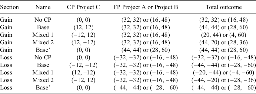
The four main treatments in the Net Gain section presented the same FPs: (32, 32) for Project A and (16, 48) for Project B in the first question. The sooner payment of Project A varied in subsequent questions to find indifference values, using the same method as in Studies 1, 2, and 3. Each treatment featured distinct CPs. The treatments named No CP and Base represented non-mixed-outcome scenarios, while Mixed 1 and Mixed 2 corresponded to mixed-outcome scenarios. Specifically:
-
• No CP treatment (non-mixed-outcome) had no CPs, represented as (0,0).
-
• Base treatment (non-mixed-outcome) included CPs of (12, 12).
-
• Mixed 1 treatment (mixed-outcome) included CPs of (–12, 12).
-
• Mixed 2 treatment (mixed-outcome) included CPs of (12, –12)
An additional treatment, named Base’, representing a specific frame of Base, shared the same total outcome as Base but without CPs (Set AC: FPs of (44, 44); Set BC: FPs of (28, 60)). In the Net Loss section, the sign of all payments for each option was inverted (see Table A1).
Parameters in the first questions for each treatment in Net Gain and Net Loss sections (Auxiliary Study)

Note: The payments in the experiments are denoted as $({M}_0,{M}_2$
), where
$({M}_0,{M}_2$
), where ${M}_0$
represents an immediate payment and
${M}_0$
represents an immediate payment and ${M}_2$
signifies a payment realized in 2 months. After the first question, the sooner payment of Project A is varied for each question based on the previous answers while the other payments remain fixed to identify their indifference points.
${M}_2$
signifies a payment realized in 2 months. After the first question, the sooner payment of Project A is varied for each question based on the previous answers while the other payments remain fixed to identify their indifference points.
The mixed-outcome effect hypothesis posits that preferences between Base and Mixed 1, as well as between Base and Mixed 2, should differ. Conversely, the cancellation hypothesis predicts that preferences across all main treatments should be identical. Additionally, to ascertain if the total outcomes influenced preferences, we examined differences between Base’ and No CP. Following the intertemporal questions, participants completed the same demographic questions as in Study 1.
The summary table of demographic variables (Auxiliary Study)

Note: The dummy variable College is assigned a value of 1 for subjects holding a college degree and 0 for those without.
A.2. Results and discussion
The demographic variables, including age, gender, and education, across the treatments were not statistically different, indicating the randomization worked properly in this study (Table A2).Footnote 8
Figure 5 presents combined boxplots and violin plots of the monthly discount factors for each treatment. The results support the cancellation hypothesis and do not endorse the mixed-outcome effect hypothesis. The IDFs did not significantly differ between the Base and Mixed 1 treatments, nor between Base and Mixed 2 in the Net Gain section (Mann–Whitney test; p = .62 and p = .48, respectively). The IDFs between Base and No CP were not significantly different either (p = .77).Footnote 9
The monthly discount factors across treatments in net gain and net loss sections (auxiliary study).
Note: Each distribution combines a violin plot and a boxplot. Violin plots are filled solid green for gain and red-striped for loss. Boxplots are overlaid in white. The bold horizontal line in each box represents the median; the bottom and top edges of the box represent the first and third quartiles, respectively. The whiskers extend to the most extreme values within 1.5 times the interquartile range (IQR).

Subsequently, further analysis was conducted to examine the effect of total outcomes as mentioned in the Method section. We showed that the IDFs between Base and No CP (treatments with identical FPs) were not significantly different in the above analysis. However, replacing Base with Base’ and retesting these treatments revealed a significant difference between Base’ and No CP (treatments with different FPs) (p < .01). The result further illustrates that the participants predominantly focused on FPs rather than total outcomes.
Similar findings were observed in the Net Loss section. The IDFs between the three pairs (Base vs. Mixed 1, Base vs. Mixed 2, and Base vs. No CP) showed no significant differences (p = .91; p = .88; p = .78, respectively), not supporting the mixed-outcome effect hypothesis either. However, the difference in IDFs between Base’ and No CP was not statistically significant (p = .57), suggesting that the difference in FPs between the two did not impact decisions in the Net Loss section. We maintained the same absolute numbers between the Net Gain and Net Loss sections for comparability. However, the magnitude of difference in FPs between Base’ and No CP in the Net Loss section might not be substantial enough to yield statistically significant results. Adjusting these values could potentially reveal significant differences. Furthermore, the time spent on decision-making between these treatments showed no significant difference (Kruskal–Wallis test; p = .47), indicating that presenting mixed outcomes did not necessarily complicate the decision-making process.
B. Appendix B: Exclusion criteria and robustness check
In our main analysis, we excluded two types of extreme observations. The first type included those that either weakly or strictly violated the principle of monotonicity across all studies, aligning with conventional methodologies for assessing individual preferences. The other type of extreme case involved observations with extreme IDFs that fell outside the intended frames. In this section, we provide detailed explanations of our exclusion criteria and the robustness check analysis in which we only excluded observations that strictly violated monotonicity.
B.1. Exclusion criteria
We excluded the first type of extreme case when participants consistently chose Project A, even when Project B (weakly) dominated A. For instance, in the Net Gain section under the No frame treatment, a participant might have chosen Set BC, which yielded £24 today and £32 in two months, over Set AC, which provided £24 today and £24 in two months. Such choices violated the principle of monotonicity, a fundamental property of preference theory, thus leading to the exclusion of these participants. There was an additional question in which Set BC (receiving £24.1 today and £32 in two months) unambiguously dominated Set AC (receiving £24 today and £24 in two months). Participants who selected Set BC in this question were included in the robustness analysis in this section.
The other type of extreme case involved participants always choosing Set BC. In that case, they would have seen, for example, Set AC (receiving £24 today and £24 in 2 months) and Set BC (receiving £8.1 today and £32 in 2 months in the Net Gain section of the No frame treatment, thus the sooner payment of project B was £0.1 in this option).Footnote 10 Although there was no theoretical reason to exclude the observations where participants chose Set BC in the example above, such choices indicated that the value in the sooner payment of Project B (note that Set BC consists of Projects B and C) would have to be negative to make Set AC and BC indifferent. However, this meant the frame of the question was no longer the same (Investment frame in this example). Therefore, we excluded observations in which participants chose Set BC in the extreme question above. Nonetheless, these preferences implied an extreme monthly IDF greater than 1.40, indicating that they made extremely patient options. Similarly, in the Net Loss section, exclusion criteria were based on violations of monotonicity and the presence of extreme IDFs that fell outside the intended frames.
B.2. Robustness check
For this robustness check, we included observations that weakly violate monotonicity and replicated the main analysis regarding IDFs. Table B1 illustrates the proportion of observations that weakly violate monotonicity in each study. The subsequent analysis demonstrated that the inclusion of these observations did not alter the overall results, thereby affirming the robustness of the findings reported in the main analysis.
The proportion of the observations that weakly violate monotonicity

B.2.1. Study 1
In line with the main analysis, framing effects were observed in both the Net Gain and Net Loss sections in Study 1. Specifically, the IDF in the No frame was statistically distinct from that in the Investment frame (Mann–Whitney test; p < .01) and the Loan frame (p < .001). In the Net Loss section, significant differences were found between the IDF in the No frame and those in the Investment frame (p = .01) and the Loan frame (p = .04).
The comparative analysis of IDFs between the Net Gain and Net Loss sections was consistent with the results of the main analysis as well. In the No frame, median IDFs were higher in the Net Loss section (Wilcoxon signed-rank test; p < .001), whereas in the Investment and Loan frames, the IDFs did not significantly differ (p = .07; p = .12).Footnote 11
B.2.2. Study 2
The overall findings from Study 2 were consistent with those of the main analysis as well and further confirmed that the framing effect was substantial and robust. First, the outcomes supported the cancellation hypothesis, as no significant differences were observed in the IDFs across the six main treatments (Kruskal–Wallis test; p = .64). The subsequent analysis further suggested that participants focused on FPs rather than total outcomes in their decisions. Specifically, no significant difference was observed in the IDFs between loan_CPD and gain_no (p = .63), while a significant difference was found between loan_CPD’ and gain_no (Mann–Whitney test; p < .001). Similarly, there was no significant difference in IDFs between inv_CPD and gain_no (p = .17), while a significant difference was found between inv_CPD’ and gain_no (Mann–Whitney test; p < .01).Footnote 12
B.2.3. Study 3
The findings from Study 3 also aligned with those of the main analysis, demonstrating that the IDF in the Loan frame was significantly different from that in the No frame (p < .01). Additionally, there was no significant difference between the IDF in the No frame and that in the Investment frame (Mann–Whitney test; p = .22).
Subsequently, we compared the results with those from the Net Gain section in Study 1. The IDFs between these studies were not statistically different in the No frame and Investment frame (Mann–Whitney test; No frame, p = .80; Investment frame, p = .21),Footnote 13 while the IDFs between the two studies were significantly different in the Loan frame (p = .04), consistent with the main analysis.
B.2.4. Auxiliary study
The findings from Auxiliary Study aligned with those of the main analysis, confirming the cancellation hypothesis. Our replication test did not support the mixed-outcome effect hypothesis. The IDFs between the Base condition and the other three main conditions (Mixed 1, Mixed 2, and No CP) showed no significant differences (p = .54, .28, and .77, respectively) in the Net Gain section.Footnote 14 Similarly, IDFs between Base and the other three main conditions were not significant (p = .91, .88, and .78, respectively) in the Net Loss section. Subsequent analysis on the effect of total outcomes was consistent with the main analysis as well. The IDF was significantly different between the Base’ and No CP treatments in the Net Gain section (p < .01) but not in the Net Loss section (p = .57).
C. Appendix C: Proportion of initial impatient choices across conditions
We conducted the main analysis using IDFs, which provide a detailed estimate of participants’ time preferences and are widely used in the time preference literature. Additionally, we also examined participants’ initial decision behavior—specifically, the proportion who chose Set AC on their first choice (the more impatient choice in the Net Gain section; Set BC, the more impatient choice in the Net Loss section) across the three main experiments. Although this approach does not offer a precise estimate of time preferences, it has the advantage of not relying on the PEST procedure. Notably, the overall results from this analysis were consistent with our main findings, providing additional support for the robustness of our conclusions.
C.1. Study 1
Table C1 presents the differences in the proportion of participants choosing Set AC across conditions and sections in Study 1. In the Net Gain section, the proportion differed significantly across treatment conditions (χ2 test, p = .001). A similar pattern was observed in the Net Loss section (p < .001).
Proportion of choosing the more impatient option in the initial choice in Study 1

Furthermore, in the No frame condition, a significantly higher proportion of participants chose the more impatient option in the Net Gain section compared with the Net Loss section (McNemar test, p < .001). This finding is consistent with the sign effect (for a review, Frederick et al., Reference Frederick, Loewenstein and O’Donoghue2002).
C.2. Study 2
Table C2 shows how the proportion of participants selecting Set AC varied across different conditions in Study 2. The overall proportion did not differ significantly across the six main treatments (χ2 test, p = .29). In addition, the comparison between loan_CPD and gain_no yielded a nonsignificant difference (p = .21), whereas the comparison between loan_CPD’ and gain_no showed a significant difference (p < .001). Similarly, the difference between inv_CPD and gain_no was not significant (p = .06), while the difference between inv_CPD’ and gain_no was significant (p = .03). These results further confirm that framing effects are primarily driven by differences in FPs, not total outcomes.
Proportion of choosing the impatient option (Project AC) in the initial choice in Study 2

C.3. Study 3
Table C3 displays the variation in the proportion of participants who chose Set AC across conditions in Study 3. The proportion differed across treatment conditions (χ2 test, p = .04). To explore this further, we conducted pairwise χ2 tests. A significant difference was found between the No frame and Loan frame conditions (p = .03), while no significant difference was observed between the No frame and Investment frame (p = .98).
Proportion of choosing the impatient option (Project AC) in Study 3


 Open access