


1. Introduction
The role of employer monopsony power in U.S. labor markets has received considerable attention from scholars and policymakers in recent years. In its review of the existing empirical monopsony literature, the U.S. Department of the Treasury (2022) concluded that the “American labor market is characterized by high levels of employer power.” The estimates that the Department of the Treasury (2022) reviewed say that labor market power is responsible for wage losses of at least 15%. The reduced wages in monopsonistic markets have potential consequences for the value of a statistical life (VSL), which is the tradeoff rate between money and fatality risks. Because the wage rate enters linearly when constructing the VSL based on semi-log wage equation estimates, one might expect that the reduced wage rate would lead to a lower VSL. Examining the relationship between monopsony and the VSL has crucial policy ramifications because the VSL is the economic price used to monetize changes in mortality risks for policies intended to reduce health, safety, and environmental risks. When noncompetitive forces reduce wages, a related concern is that noncompetitive forces may also reduce the VSL (Kniesner & Viscusi, Reference Kniesner and Viscusi2023). Monopsony may also have adverse effects on workers if it increases the level of job risk, as theorized in Viscusi (Reference Viscusi1980). Our focus here is not on the overall effect of monopsony on worker welfare but on the effect of monopsony on the VSL. This article presents the first evidence concerning the relationship of monopsony to the VSL, which we find varies across labor market contexts and is greater in highly concentrated U.S. labor markets. Our focal result reduces concerns that the VSL is distorted and underestimated because of labor market noncompetition. As will be discussed in the concluding Section 5, there is also no compelling case for adjusting the average VSL for the impact of monopsony.
Labor market estimates of the VSL usually use a semi-logarithmic wage equation specification for which the calculated VSL is based on the product of the wage rate and the regression parameter capturing the marginal price of job safety (Viscusi & Aldy, Reference Viscusi and Aldy2003). Employer monopsony power – either through its direct wage effects or through its effects on the marginal price of safety – could be a source of heterogeneity in commonly used VSL estimates. To assess the degree of noncompetitive effects on VSL, we use the restricted access Census of Fatal Occupational Injuries (CFOI) files to construct granular fatality risk measures in conjunction with a Herfindahl–Hirschman Index (HHI) that measures the local concentration of online job vacancy postings within occupations (Choi & Marinescu, Reference Choi and Marinescu2023).
Prior research evaluates the wage impacts of employer monopsony power using a wide range of empirical strategies, generally finding that increased labor market power reduces wages. Multiple articles exploit cross-sectional variation in wages and local industry- or occupation-based concentration measures (Azar et al., Reference Azar, Marinescu, Steinbaum and Taska2020; Azar et al., Reference Azar, Marinescu and Steinbaum2022; Rinz, Reference Rinz2022; Handwerker & Dey, Reference Handwerker and Dey2023; Qiu & Sojourner, Reference Qiu and Sojourner2023; Jarosch et al., Reference Jarosch, Nimczik and Sorkin2024).Footnote 1 Our empirical approach is most similar in spirit to their research, as we focus on the effects of monopsony power stemming from market structure and local competition for labor on the hedonic wage-risk equilibrium.Footnote 2
The substantial and growing body of research has influenced the economic policy priorities of various divisions of the federal government, particularly under the Biden administration. Alongside the U.S. Department of the Treasury’s (2022) assessment, the 2022 Economic Report of the President identifies monopsony power as a barrier to economic equality: “[p]erfect competition does not describe most labor markets … [T]he market power of employers … allows for unfair hiring and compensation practices” (Council of Economic Advisers, 2022). The 2023 Merger Guidelines commit the competition agencies to consider the effects of mergers on labor markets and workers (U.S. Department of Justice and Federal Trade Commission, 2023).Footnote 3 And the now-rescinded 2023 U.S. Office of Management and Budget’s Circular A-4 regulatory analysis guidance notes that “market power may affect … benefit and cost estimates” and requires agencies to consider how regulations may strengthen or limit “labor market competition in ways that impact workers” (U.S. Office of Management and Budget, 2023).
The most acute policy concern in our context here is whether employer monopsony power is a source of downward bias in the VSL estimates that are prevalent in the administrative state’s benefit–cost analyses. Prior research finds that for some disadvantaged labor groups, such as Black individuals and Mexican immigrants, the VSL is smaller than conventional uniform VSL estimates that reflect the entire population (Viscusi, Reference Viscusi2003; Hersch & Viscusi, Reference Hersch and Viscusi2010). The results just mentioned are consistent with a formulation of the labor market where disadvantaged groups face a distinct, segmented market opportunities locus that is lower and flatter. Consequently, the disadvantaged population receives less compensation for marginal fatality risks. In these situations, workers locate their job choice on their available market opportunities locus, and that choice reflects their local preferences. Worker preferences do not change because of monopsony. Workers’ constant iso-expected utility curves are the same irrespective of market opportunities. But if workers in monopsonistic industries had access to a different set of options, the observed tradeoff rate based on their job choice from a non-monopsony market offer curve might be different. That policymakers would want to base the VSL on a counterfactual situation in which workers faced market offer curves different than those that they currently encounter in the market is unlikely, whether the context involves monopsony or potential labor market discrimination. In the absence of a demonstrable major market failure that differences in monopsony distort estimates the average VSL, the application of the average VSL is likely to continue to prevail.
Given that employer monopsony power seems to disadvantage workers in terms of wages and working conditions, the notion that employer monopsony power would decrease the VSL has some intuitive appeal. Our results, however, strongly refute this. Instead, we find that the implied VSL is larger in highly concentrated, oligopsonistic labor markets. That is, workers in oligopsonistic labor markets receive more compensation for additional risk. A higher compensation for risk is consistent across several different econometric approaches. A reassuring aspect of the results for the use of labor market estimates of the VSL in policy analyses is that the usual set of controls for industry and occupation in all recent labor market studies using the CFOI data will capture the influence of monopsonistic factors correlated with industry or occupation.
Though workers in more concentrated markets are not shortchanged in terms of compensating differentials for occupational fatality risks, in equilibrium, the increased marginal price of safety and decreased wages associated with monopsony power will lead workers in more concentrated labor markets to be in more dangerous jobs. The focus of our analysis is on the VSL tradeoff rate, not on the level of job risks or work quality more generally, which is a separate issue.
The effect of differences in labor market structure on compensating differentials for risk is also evident in labor market studies of the effect of unemployment rates. Guo and Hammitt (Reference Guo and Hammitt2009) find that for Chinese labor markets, the interaction term of unemployment rates × fatality risk in the wage equation is negative. Increased regional unemployment rates are correlated with lower rates of compensation for mortality risks. High unemployment both reduces the wage rate, as is also the case with monopsony, and high unemployment also lowers the VSL. This relationship has also been borne out in several other studies. Using U.S. Current Population Survey (CPS) data, Bender and Mridha (Reference Bender and Mridha2011) find that areas with high metro unemployment have lower compensation rates for lost workday injury rates, implying a lower value of a statistical injury. Mridha and Khan (Reference Mridha and Khan2013) find a similar depressing effect of SMSA regional employment rates on the wage premium for fatality risks based on U.S. CPS data and SMSA unemployment rates. Leeahtam et al. (Reference Leeahtam, Leurcharusmee, Jatukannyaprateep, Huynh, Kreinovich and Sriboonchitta2014) also find an adverse effect of high unemployment (i.e. the difficulty of finding a job within three months) in Thailand, which is negatively related to the worker’s self-reported exposure to occupational hazards. The consistency of these findings bolsters the recommendation by Guo and Hammitt (Reference Guo and Hammitt2009) that it is invalid to use the overall VSL if high societal unemployment rates bias the VSL downwards. The focus of the current article is on whether there is a depressing effect of monopsony on the VSL that would warrant a similar type of adjustment.
Our discussion continues as follows. Section 2 visualizes how employer monopsony power could impact the VSL and explains our estimating equations. Section 3 details the CPS MORG and NLSY97 employment samples, the construction of the fatality rate variable from the CFOI files, and the HHI measure. Section 4 presents our regression results using the CPS MORG and NLSY97 employment samples using the first differences model advocated in Kniesner et al. (Reference Kniesner, Viscusi, Woock and Ziliak2012). Section 5 concludes.
2. Conceptual framework and estimation strategy
2.1. VSL estimation and inference
Our principal VSL estimating equation is:


where
$ \log \left( wag{e}_{it}\right) $
 is the natural logarithm of hourly wages for person
$ i $
is the natural logarithm of hourly wages for person
$ i $
 in year
$ t $
in year
$ t $
 . The fatality risk variable is assigned based on each worker’s occupation
$ o $
. The fatality risk variable is assigned based on each worker’s occupation
$ o $
 and industry
$ j $
and industry
$ j $
 at time
$ t $
at time
$ t $
 , and
$ HH{I}_{cot} $
, and
$ HH{I}_{cot} $
 is assigned based on the worker’s commuting zone
$ c $
is assigned based on the worker’s commuting zone
$ c $
 , occupation
$ o $
, occupation
$ o $
 , and time
$ t $
, and time
$ t $
 .
$ {X}_i $
.
$ {X}_i $
 is a vector of individual-level controls detailed below in the Data section. State, major occupation group, and year fixed effects are represented by
$ {\delta}_s $
is a vector of individual-level controls detailed below in the Data section. State, major occupation group, and year fixed effects are represented by
$ {\delta}_s $
 ,
$ {\gamma}_o $
,
$ {\gamma}_o $
 , and
$ {\pi}_t $
, and
$ {\pi}_t $
 , respectively. In some regressions, we include a set of interaction terms between major occupation group and local concentration, represented by
$ {\gamma}_o\ast \log \left( HH{I}_{cot}\right) $
, respectively. In some regressions, we include a set of interaction terms between major occupation group and local concentration, represented by
$ {\gamma}_o\ast \log \left( HH{I}_{cot}\right) $
 , which allows for heterogeneous wage effects of concentration by job type.
Using a 2000-hour work year, the VSL is calculated using the following formula:

where
$ \hat{\theta} $
 is the average marginal effect of
$ FatalityRis{k}_{ojt} $
is the average marginal effect of
$ FatalityRis{k}_{ojt} $
 on
$ \log \left( wag{e}_{it}\right) $
on
$ \log \left( wag{e}_{it}\right) $
 . In conventional VSL estimation,
$ \hat{\theta} $
. In conventional VSL estimation,
$ \hat{\theta} $
 is equal to the estimated coefficient of the fatality risk variable. The inclusion of interactions between concentration and risk in our context requires us to instead use average marginal effects. In parts of our analysis, we set
$ \hat{\theta} $
is equal to the estimated coefficient of the fatality risk variable. The inclusion of interactions between concentration and risk in our context requires us to instead use average marginal effects. In parts of our analysis, we set
$ \hat{\theta} $
 equal to the marginal effect of fatality risk on wages at various points in the log(HHI) distribution (30th percentile, median, and 70th percentile). In specifications with an interaction between
$ FatalityRis{k}_{ojt} $
equal to the marginal effect of fatality risk on wages at various points in the log(HHI) distribution (30th percentile, median, and 70th percentile). In specifications with an interaction between
$ FatalityRis{k}_{ojt} $
 and binary variables reflecting concentration levels (
$ {\beta}_1 FatalityRis{k}_{ojt}+{\beta}_2{HighlyConcentrated}_{cot}+{\beta}_3\left[ FatalityRis{k}_{ojt}\times {HighlyConcentrated}_{cot}\right] $
and binary variables reflecting concentration levels (
$ {\beta}_1 FatalityRis{k}_{ojt}+{\beta}_2{HighlyConcentrated}_{cot}+{\beta}_3\left[ FatalityRis{k}_{ojt}\times {HighlyConcentrated}_{cot}\right] $
 ), we set

In our main CPS regressions, we account for serial correlation in wages by job type and broad geography by clustering standard errors by state, industry, and occupation (Viscusi & Gentry, Reference Viscusi and Gentry2015).Footnote
4 Further, VSL standard errors are computed using the following variance formula from Kniesner et al. (Reference Kniesner, Viscusi, Woock and Ziliak2012):
$ Var(VSL)={\mathrm{100,000}}^2\times {\mathrm{2,000}}^2\times {\left( mean(wage)\right)}^2\times Var\left({\beta}_1\right) $
 , where
$ {\beta}_1 $
, where
$ {\beta}_1 $
 is the estimated fatality risk parameter. For models that include interactions between fatality risk and log(HHI), we replace
$ Var\left({\beta}_1\right) $
is the estimated fatality risk parameter. For models that include interactions between fatality risk and log(HHI), we replace
$ Var\left({\beta}_1\right) $
 in the above variance equation with the variance of a nonlinear combination of regression parameters, estimated using the delta method, of the following form:
$ \Big[{\beta}_1+f\left(\log (HHI)\right)\times {\beta}_3 $
in the above variance equation with the variance of a nonlinear combination of regression parameters, estimated using the delta method, of the following form:
$ \Big[{\beta}_1+f\left(\log (HHI)\right)\times {\beta}_3 $
 ] (Gian et al., Reference Gian, Gupta, Simon, Sullivan and Wing2024). The function
$ f\left(\log (HHI)\right) $
] (Gian et al., Reference Gian, Gupta, Simon, Sullivan and Wing2024). The function
$ f\left(\log (HHI)\right) $
 takes either the mean, median, 30th percentile, or 70th percentile of the
$ \log (HHI) $
takes either the mean, median, 30th percentile, or 70th percentile of the
$ \log (HHI) $
 distribution, as indicated in the tables. If we use a dummy variable reflecting concentration such as
$ {HighlyConcentrated}_{cot} $
distribution, as indicated in the tables. If we use a dummy variable reflecting concentration such as
$ {HighlyConcentrated}_{cot} $
 , we replace
$ f\left(\log (HHI)\right) $
, we replace
$ f\left(\log (HHI)\right) $
 with
$ mean\left({HighlyConcentrated}_{cot}\right) $
with
$ mean\left({HighlyConcentrated}_{cot}\right) $
 .
.
2.2. Possible effects of monopsony power on the VSL
The VSL depends on the wage rate and the estimated slope of the hedonic wage-risk locus. We have clear predictions regarding the effect of employer monopsony power on the wage rate based on prior empirical work. Greater labor market concentration is typically associated with lower wages, which we will also find in our data.Footnote 5
Because the VSL is calculated based on the product of the wage rate and the slope of the wage–fatal injury risk relationship, assessing whether the VSL is higher or lower with monopsony depends on both of these components. Since monopsony reduces worker wages if there is no statistically significant interactive effect in Equation (1), or if this interaction term is negative, then monopsony definitely reduces the VSL. If, however, monopsony boosts the wage–fatal injury risk tradeoff, then the effect of monopsony on the VSL is ambiguous.
Figure 1 illustrates the possibilities. In every case, worker preferences remain unchanged. But the VSL that is reflected in the choices that workers make from the available market opportunities locus is different in the situations shown in Figure 1. There is no reason to assume a priori that the market opportunities locus for monopsony would lead workers to choose jobs with a higher or lower VSL. The observed VSL for workers may depend on how the market opportunities locus differs in monopsonistic markets. The top line in Figure 1 reflects the competitive market reference point for which there is a higher base wage rate. Point A on this curve indicates the competitive market wage rate for the fatality rate p* in the sample. The three lower lines in Figure 1 indicate the different possibilities for the interactive effect of monopsony and fatality risks, where point B indicates the market fatality rate and sample wage rate for monopsonistic firms at the intersection of possible monopsony tradeoff rate curves. The lowest monopsony tradeoff rate line is flatter than that for competition, in which case the VSL under monopsony will definitely be lower. The middle monopsony tradeoff rate line has the same slope as the competitive market line. Coupling the same slope with a lower wage rate under monopsony will generate a lower VSL for monopsony than for the competitive market. The top monopsony tradeoff rate is steeper than that in the competitive case, which will reduce or potentially reverse the adverse wage effect of monopsony on the VSL. The empirical results below are consistent with the top line in Figure 1, which has a steeper tradeoff rate.
The effect of monopsony = Wage × Slope.

Figure 1. Long description
The horizontal axis is labeled fatal injury rate, with a vertical dashed line at p star. The vertical axis is labeled ln w. The competitive wage line slopes upward from left to right, passing through point A above the intersection. Point B marks the intersection of the horizontal line and the vertical dashed line at p star. Three lines radiate from B: one labeled VSL same or higher, one labeled VSL lower, and one labeled VSL lower with an underline. A bracket on the right groups these three lines as 3 possible monopsony cases. The competitive wage line is above all three monopsony lines at p star.
3. Data
3.1. CPS MORG employment sample
Our primary employment sample is the 2011–2021 Current Population Survey Merged Outgoing Rotation Group (CPS MORG) extracts provided by IPUMS (Flood et al., Reference Flood, King, Rodgers, Ruggles, Warren, Backman, Chen, Cooper, Richards, Schouweiler and Westberry2024). The sample consists of respondents aged 16 to 70 who work at least 35 hours a week. We drop self-employed, agricultural, and military workers. Our dependent variable is hourly wages in 2022 dollars.Footnote 6 If hourly wage data are not provided for a certain respondent, we impute weekly earnings divided by usual weekly hours.Footnote 7 As is standard in VSL estimation studies, we exclude persons with an hourly wage below $2 or above $100 to mitigate the influence of outliers.Footnote 8
Our empirical analysis controls for a wide range of demographic variables, including sex, race, education, marital status, metropolitan status, potential work experience and its square,Footnote 9 and whether the respondent is paid hourly, covered by a union, or works for the government. The education variable is a slightly recoded version of the IPUMS educational attainment variable to approximate years of education.Footnote 10 We also control for annual two-digit NAICS industry nonfatal injury and illness rates using public data on the lost workday injury and illness rate for cases involving a lost workday from the U.S. Bureau of Labor Statistics (BLS).Footnote 11 The final sample, which is summarized in Table 1, consists of 1,329,085 observations that are not missing any of the key variables.
CPS summary statistics

Table 1. Long description
The table has three columns: VARIABLES, Mean, and SD. From top to bottom, variables and their mean and SD values are: Hourly wage in 2022 dollars, 29.35 and 17.62; HH I, 1,958 and 2,054; Highly concentrated HHI greater than 2,500 (zero or one), 0.290 and 0.454; Male (zero or one), 0.551 and 0.497; White (zero or one), 0.779 and 0.415; Black (zero or one), 0.127 and 0.333; Native American (zero or one), 0.00975 and 0.0983; Asian (zero or one), 0.0627 and 0.242; Multiracial (zero or one), 0.0174 and 0.131; Hispanic ethnicity (zero or one), 0.168 and 0.374; Potential experience, 22.77 and 12.86; Years of education, 13.95 and 2.514; Married (zero or one), 0.585 and 0.493; Paid hourly (zero or one), 0.536 and 0.499; Union (zero or one), 0.135 and 0.342; Government worker (zero or one), 0.165 and 0.371; Metropolitan status (zero or one), 0.880 and 0.325; Injury and illness rate per 100,000, 1,003 and 541.2; Missing injury and illness rate (zero or one), 0.00389 and 0.0622. All variables have N equals 1,329,085. Data are from CPS Merged Outgoing Rotation Group extracts, 2011 to 2021, with earnings weights applied. For missing injury and illness rate data, the rate is set to zero and a dummy variable is included.
Notes: N = 1,329,085 for all variables. Summary statistics from the CPS Merged Outgoing Rotation Group extracts provided by IPUMS (2011–2021). Results reflect CPS earnings weights. For the small number of observations with missing injury and illness rate data, we set the injury and illness rate equal to zero and include a separate dummy variable.
3.2. NLSY97 employment sample
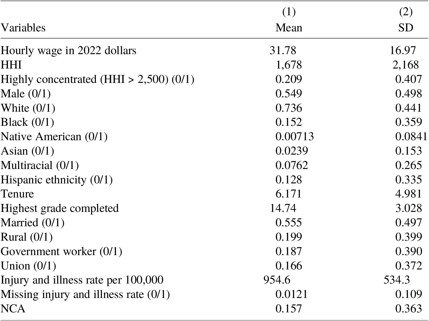
To complement the main CPS MORG employment sample, we also use Rounds 18, 19, and 20 of the National Longitudinal Survey of Youth 1997 (NLSY97). Though the NLSY97 is much smaller than the CPS MORG, the advantage of the NLSY97 is that it includes information on the county of every respondent in each survey year using the restricted-access geocode file, making it possible to match measures of labor market concentration to the worker’s local labor market. (In the CPS MORG, county information is suppressed for respondents in smaller population counties.) Summary statistics for the NLSY97 are presented in Appendix Table A1.Footnote 12
3.3. Fatality rate variable construction
We construct hours-based fatality rates using restricted access data from the BLS’s CFOI files, which provide a comprehensive count of all work-related fatalities that have been corroborated using multiple data sources. For reference, the public CFOI national fatal work injury rate was 3.5 fatalities per 100,000 full-time workers in 2023 (U.S. Bureau of Labor Statistics, 2024).Footnote 13 Disclosure restrictions prevent the release of the fatality rate in the sample used in our study, but our sample was broadly representative of the U.S. workforce. Our constructed fatality rate variable differs by both industry and occupation. In total, we have 1,030 potential annual industry-occupation cells, based on 103 industries and 10 major occupation groups. The 103 industries include 97 three-digit NAICS industry classifications and six select two-digit NAICS industries.Footnote 14 The 10 major occupation groups correspond to the census major occupation group aggregations,Footnote 15 omitting the Armed Forces category.
We calculate a moving three-year average fatality rate to provide a more precise measure of the low-probability risk and to reduce the number of empty cells without any fatalities. The fatality rate variable otherwise accords with BLS documentation (Northwood, Reference Northwood2010) and uses the following equation:

For any given year, the numerator
$ N $
 equals the sum of all fatalities in the CFOI of non-volunteer, non-military individuals over age 16 in the relevant industry-occupation cell occurring in that year and the prior two years. The denominator of the fatality risk variable,
$ EH $
equals the sum of all fatalities in the CFOI of non-volunteer, non-military individuals over age 16 in the relevant industry-occupation cell occurring in that year and the prior two years. The denominator of the fatality risk variable,
$ EH $
 , is the estimated total hours of work performed by all employees in an industry and occupation category in the same three years.Footnote
16
, is the estimated total hours of work performed by all employees in an industry and occupation category in the same three years.Footnote
16
Though there are 1,030 possible industry-occupation cells in any year the actual number of calculated fatality rate cells each year is smaller. The smaller number of calculated fatality rate cells happens because there must be at least one individual in the CPS within that industry and occupation to generate the denominator. From 2011–2021, there are 9,180 total fatality rate cells (an annual average of around 835 annual cells).
Although the fatality rate data reflect differences by occupation and industry, the confidential data to which we had access did not include geographic information. Thus, differences in the risk across local labor markets would be a potential source of measurement error. If this measurement error is negatively correlated with the HHI so that the local risk in the high HHI markets is higher than the calculated national average risk, the error will tend to bias the estimates of the VSL, leading to an overestimation of the VSL in high HHI markets.
3.4. Local labor market concentration data
We generally define labor markets as a six-digit SOC occupation and commuting zone, which is a commonly used approach throughout the monopsony literature (Azar et al., Reference Azar, Marinescu, Steinbaum and Taska2020; Azar et al., Reference Azar, Marinescu and Steinbaum2022; Handwerker & Dey, Reference Handwerker and Dey2023; Azar et al., Reference Azar, Huet-Vaughn, Marinescu, Taska and Von Wachter2024).Footnote 17 Commuting zones are collections of adjacent counties that approximate local economies. Occupational mobility within six-digit SOC occupations is relatively low; 76% of job changers remain in the same six-digit SOC occupation (Schubert et al., Reference Schubert, Stansbury and Taska2024). This suggests six-digit SOC occupations are a reasonable way of defining labor markets.
Our source of labor market concentration data is Choi and Marinescu (Reference Choi and Marinescu2023).Footnote 18 The same data have been used in multiple prior labor monopsony papers (Azar et al., Reference Azar, Marinescu, Steinbaum and Taska2020; Azar et al., Reference Azar, Huet-Vaughn, Marinescu, Taska and Von Wachter2024). To calculate the labor market HHI for each market, Choi and Marinescu measure each firm’s share of online job vacancy postings. The online job vacancy posting data is from Lightcast (formerly Burning Glass Technologies). The HHI is the sum of the squares of each firm’s share of online job vacancy postings. Azar et al. (Reference Azar, Marinescu, Steinbaum and Taska2020) believe that a vacancy-based concentration measure is more appropriate than employment-based measures because “workers remain in jobs for longer,” so “concentration of employment may be a less relevant gauge of available work and employer market power than is the concentration of vacancies among the relatively few firms who are likely to be hiring.” We use Choi and Marinescu’s “lower-bound” HHI estimates, which assumes each online job vacancy with a missing employer name is distinct from every other missing employer and all identified employers (Choi & Marinescu, Reference Choi and Marinescu2023). Because the Choi and Marinescu data are quarterly, we take the unweighted average across all quarters to generate an annual HHI estimate for each labor market.Footnote 19
Further details on the procedures used to prepare the Choi and Marinescu (Reference Choi and Marinescu2023) data for the CPS MORG and NLSY97 analysis are available in Technical Appendix 1. There we also explain our strategy for assigning HHI data to the large proportion of respondents in the CPS MORG that lack county identifiers.
4. Results
4.1. CPS MORG results
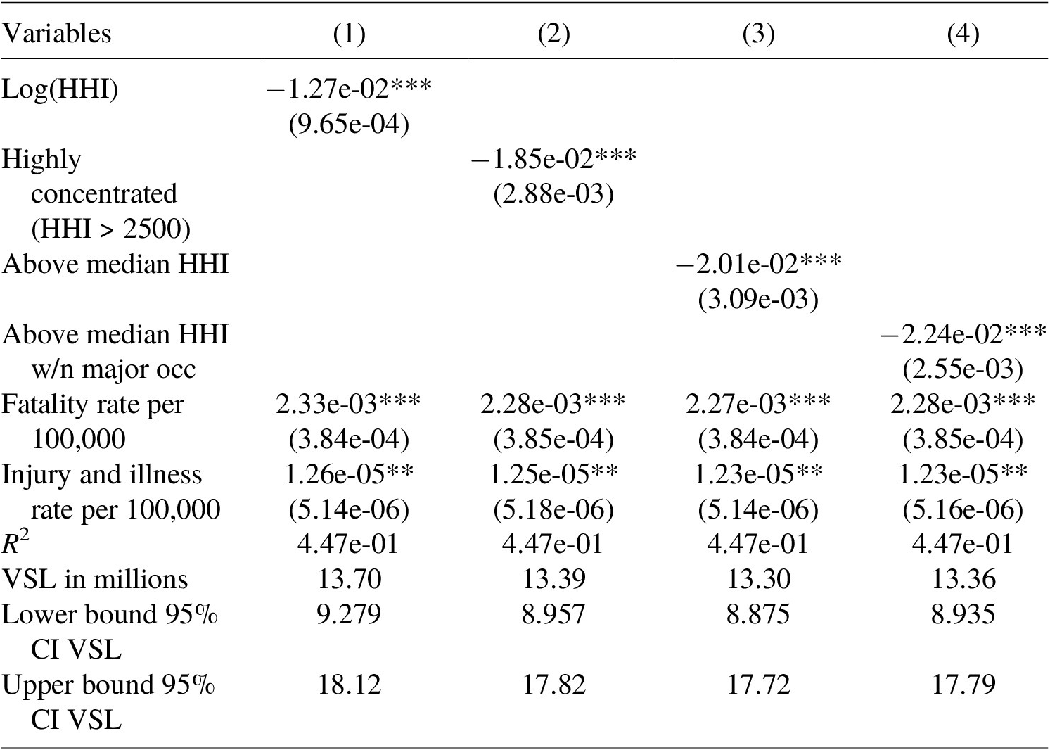
Table 2 presents results from a series of hedonic wage regressions that include fatal risk measures, nonfatal risk measures, and various labor market concentration measures. The coefficient on each concentration measure is negative and statistically significant at the one percent level, suggesting that increased concentration is associated with lower wages. The association is consistent with the findings of most of the existing empirical literature. The fatal and nonfatal risk measures are positive and statistically significant at the one and five percent level, respectively, corroborating the existence of meaningful compensating differentials for broad categories of occupational hazards. The implied VSL ranges from $13.3 million to $13.7 million and appears stable regardless of which variant of the concentration measure is employed.
Log wage regressions on concentration and risk measures

Table 2. Long description
Beginning at the top row, the table displays four columns labeled one, two, three, and four. The first column lists variables: Log HH I, Highly concentrated (H HI greater than 2500), Above median HH I, Above median HHI within major occupation, Fatality rate per 100,000, Injury and illness rate per 100,000, R squared, VSL in millions, Lower bound 95 percent CI VS L, and Upper bound 95 percent CI VSL. Log HHI shows a coefficient of minus 1.27 times 10 to the minus 2, standard error 9.65 times 10 to the minus 4, significant at p less than 0.01, in column one. Highly concentrated HHI greater than 2500 has a coefficient of minus 1.85 times 10 to the minus 2, standard error 2.88 times 10 to the minus 3, significant at p less than 0.01, in column two. Above median HHI yields minus 2.01 times 10 to the minus 2, standard error 3.09 times 10 to the minus 3, significant at p less than 0.01, in column three. Above median HHI within major occupation gives minus 2.24 times 10 to the minus 2, standard error 2.55 times 10 to the minus 3, significant at p less than 0.01, in column four. Fatality rate per 100,000 is positive across all columns: 2.33 times 10 to the minus 3, 2.28 times 10 to the minus 3, 2.27 times 10 to the minus 3, and 2.28 times 10 to the minus 3, all significant at p less than 0.01, with standard errors ranging from 3.84 to 3.85 times 10 to the minus 4. Injury and illness rate per 100,000 is positive in all columns: 1.26 times 10 to the minus 5, 1.25 times 10 to the minus 5, 1.23 times 10 to the minus 5, and 1.23 times 10 to the minus 5, significant at p less than 0.05, with standard errors from 5.14 to 5.18 times 10 to the minus 6. R squared is 4.47 times 10 to the minus 1 in all columns. VSL in millions ranges from 13.70 in column one to 13.36 in column four. Lower bound 95 percent CI VSL ranges from 9.279 to 8.935, upper bound from 18.12 to 17.79. Notes indicate N equals 1,329,085, standard errors are clustered, significance levels are denoted by asterisks, and controls include demographic and employment variables.
Notes: N = 1,329,085. Results reflect CPS earnings weights except for calculating the various median HHI levels. Standard errors clustered by state, major occupation group, and 3-digit NAICS industry in parentheses, ***p < 0.01, **p < 0.05, *p < 0.1. Each regression also includes controls for sex, race, reporting Hispanic ethnicity, education, marital status, metropolitan status, potential work experience, potential work experience squared, and whether the respondent is paid hourly, covered by a union, or works for the government. We also include a dummy variable if missing 2-digit NAICS industry nonfatal injury and illness rate and state, year, and major occupation group fixed effects. The sample mean wage is used to calculate the VSL.
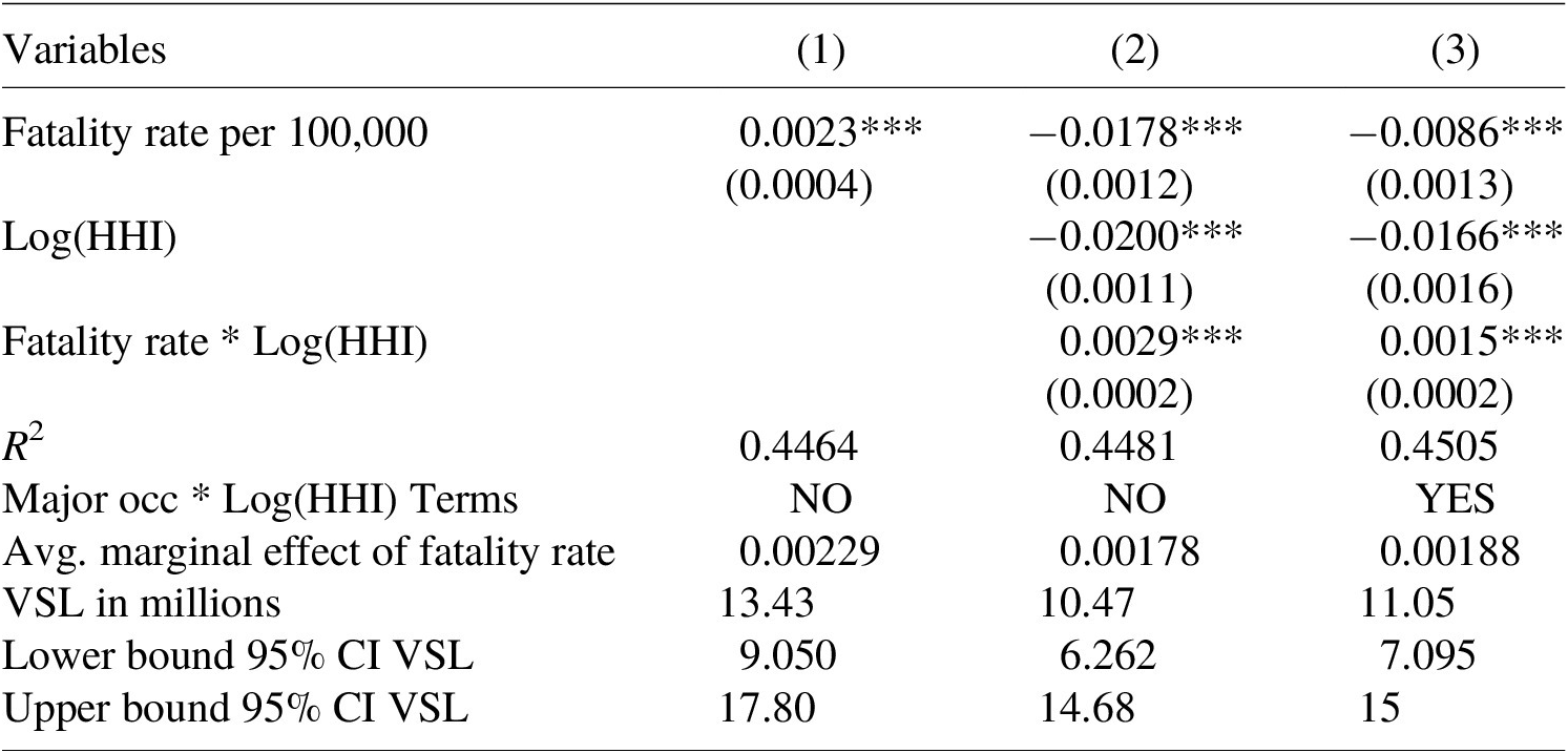
We next examine how the implied VSL differs when allowing the fatality rate to vary by concentration levels. Column 1 of Table 3, which includes neither concentration measures nor fatality risk interaction terms and serves as a reference point for conventional estimation, provides our benchmark VSL of $13.43 million. For context, a recent meta-analysis of CFOI-based VSL studies calculates a mean “best-set” VSL of $12.74 million and mean “all-set” VSL of $14.15 million (Viscusi, Reference Viscusi2018; Kniesner et al., Reference Kniesner, Sullivan and Viscusi2024).Footnote 20 Our baseline VSL is also in line with estimates used by government agencies for valuing the benefits of mortality reductions in regulatory analyses. The U.S. Department of Transportation, for instance, employed a VSL of $12.5 million in 2022 dollars (U.S. Department of Transportation, 2024).
Log wage regressions on fatality rate, with and without concentration interactions

Table 3. Long description
Beginning at the top, the table has three columns labeled (1), (2), and (3), each representing a regression specification. The first row lists ‘Fatality rate per 100,000’ with coefficients: 0.0023 triple asterisk in column (1), minus 0.0178 triple asterisk in column (2), and minus 0.0086 triple asterisk in column (3). Standard errors are shown below: 0.0004, 0.0012, and 0.0013 respectively. The next row, ‘Log(H HI)’, is blank in column (1), with coefficients minus 0.0200 triple asterisk in column (2) and minus 0.0166 triple asterisk in column (3), standard errors 0.0011 and 0.0016. The interaction term ‘Fatality rate times Log(HHI)’ is blank in column (1), with coefficients 0.0029 triple asterisk in column (2) and 0.0015 triple asterisk in column (3), standard errors 0.0002 for both. R squared values are 0.4464, 0.4481, and 0.4505. ‘Major occ times Log(HHI) Terms’ is ‘NO’ in columns (1) and (2), ‘YES’ in column (3). ‘Avg. marginal effect of fatality rate’ is 0.00229, 0.00178, and 0.00188. ‘VSL in millions’ is 13.43, 10.47, and 11.05. ‘Lower bound 95 percent CI VSL’ is 9.050, 6.262, and 7.095. ‘Upper bound 95 percent CI VSL’ is 17.80, 14.68, and 15. Notes below specify N equals 1,329,085, CPS earnings weights, standard errors clustered by state, major occupation group, and three-digit NAICS industry, significance levels, and included controls. Column (3) adds major occupation group by log(HHI) interactions, omitting management, business, and financial group. VSL confidence intervals use the delta method, with sample mean wage for calculation.
Notes: N = 1,329,085. Results reflect CPS earnings weights. Standard errors clustered by state, major occupation group, and 3-digit NAICS industry in parentheses, ***p < 0.01, **p < 0.05, *p < 0.1. Each regression also includes controls for sex, race, reporting Hispanic ethnicity, education, marital status, metropolitan status, potential work experience, potential work experience squared, and whether the respondent is paid hourly, covered by a union, or works for the government. We also include 2-digit NAICS industry nonfatal injury and illness rates (with a dummy if missing in any year) and state, year, and major occupation group fixed effects. In column 3, we include an additional set of interaction terms between each major occupation group and log(HHI) (omitting the management, business, and financial occupation group interaction). VSL confidence intervals are computed following Kniesner et al. (Reference Kniesner, Viscusi, Woock and Ziliak2012), where the variance of the fatality risk parameter for the interaction models is estimated using the delta method. The sample mean wage is used to calculate the VSL.
Column 2 adds a continuous concentration measure and an interaction term between fatal risk and concentration. The VSL, which is calculated by setting
$ \hat{\theta} $
 in Equation (2) equal to the average marginal effect of fatality risk from the regression equation, is $10.47 million. In column 3, we further augment the estimating equation with a set of interaction terms between each major occupation group and log(HHI), allowing for heterogeneous wage impacts of labor market concentration by broad occupational classification. The estimated VSL in column 3 is $11.05 million and quite close to the estimate in column 2. Allowing for the fatality risk variable to vary by concentration levels and evaluating the VSL using the average marginal effect of fatality risk on wages yields a modestly smaller VSL than values from conventional estimating equations. All the implied VSLs in Table 3, however, fall well within each other’s 95% confidence intervals.
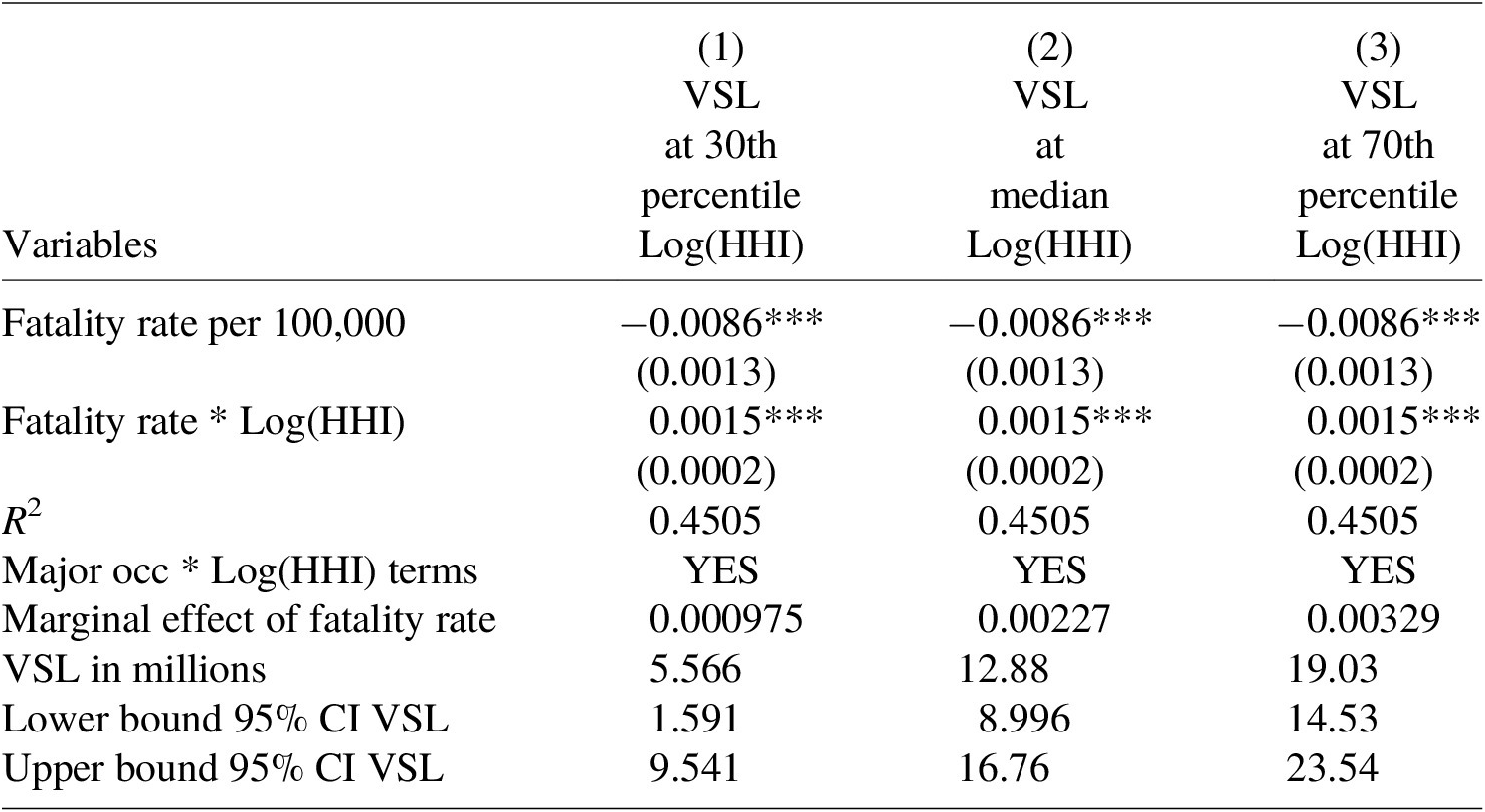
While Table 3 compares the VSL with and without concentration controls, Table 4 examines how the VSL changes at different focal values in the distribution of labor market concentration scores. Here, we calculate the VSL by setting
$ \hat{\theta} $
 equal to the marginal wage effect of fatality risk at different representative values of the log(HHI) distribution – namely, the 30th, 50th, and 70th percentiles. Additionally, to directly account for the independent effects of monopsony power on wages in the VSL calculation, in Table 4, we replace
$ \overline{Wage} $
equal to the marginal wage effect of fatality risk at different representative values of the log(HHI) distribution – namely, the 30th, 50th, and 70th percentiles. Additionally, to directly account for the independent effects of monopsony power on wages in the VSL calculation, in Table 4, we replace
$ \overline{Wage} $
 in Equation (2) (the overall sample mean wage) with the mean wage across observations in the second, third, and fourth log(HHI) quintiles, respectively, for columns 1, 2, and 3. Note that the 30th percentile of the log(HHI) distribution is the midpoint of the second log(HHI) quintile, the median is the midpoint of the third quintile, and the 70th percentile is the midpoint of the fourth quintile. The regression equation in Table 4 further includes the major occupation group and concentration interaction terms, so the specification is identical to column 3 of Table 3.
Log wage regressions on fatality rate with concentration interaction, evaluating VSL at different concentration levels

Table 4. Long description
From left to right, columns represent VSL at the 30th percentile, median, and 70th percentile. Each column lists variables: Fatality rate per 100,000 with coefficient minus 0.0086 triple asterisk and standard error 0.0013; Fatality rate times log HHI with coefficient 0.0015 triple asterisk and standard error 0.0002. R squared is 0.4505 for all columns. Major occupation times log HHI terms are marked as yes. Marginal effect of fatality rate is 0.000975 at 30th percentile, 0.00227 at median, 0.00329 at 70th percentile. VSL in millions is 5.566, 12.88, and 19.03 respectively. Lower bound 95 percent confidence interval VSL is 1.591, 8.996, and 14.53; upper bound is 9.541, 16.76, and 23.54. Notes specify N equals 1,329,085, results reflect CPS earnings weights, standard errors clustered by state, major occupation group, and three-digit NAICS industry. Significance levels are triple asterisk for p less than 0.01, double asterisk for p less than 0.05, single asterisk for p less than 0.1. Controls include sex, race, Hispanic ethnicity, education, marital status, metropolitan status, potential work experience and its square, hourly pay, union coverage, government employment, two-digit NAICS industry nonfatal injury and illness rates, state, year, major occupation group fixed effects, standalone log HHI term, and interaction terms between major occupation group and log HH I, omitting management, business, and financial occupation group interaction. VSL confidence intervals are computed using the delta method. Columns use mean wage across observations in the second, third, and fourth log HHI quintiles to calculate VS L.
Notes: N = 1,329,085. Results reflect CPS earnings weights. Standard errors clustered by state, major occupation group, and 3-digit NAICS industry in parentheses, ***p < 0.01, **p < 0.05, *p < 0.1. Each regression also includes controls for sex, race, reporting Hispanic ethnicity, education, marital status, metropolitan status, potential work experience, potential work experience squared, and whether the respondent is paid hourly, covered by a union, or works for the government. We also include 2-digit NAICS industry nonfatal injury and illness rates (with a dummy if missing in any year), state, year, and major occupation group fixed effects, a standalone log(HHI) term, and a set of interaction terms between each major occupation group and log(HHI) (omitting the management, business, and financial occupation group interaction). VSL confidence intervals are computed following Kniesner et al. (Reference Kniesner, Viscusi, Woock and Ziliak2012), where the variance of the fatality risk parameter for the interaction models is estimated using the delta method. Columns 1, 2, and 3 use the mean wage across observations in the second, third, and fourth log(HHI) quintiles, respectively, to calculate the VSL.
Table 4 shows that the VSL is larger in more concentrated labor markets. The VSL at the 30th percentile of the log(HHI) distribution is $5.57 million. This is close to the 10th percentile of the distribution of CFOI-based, all-set VSL estimates from the meta-analyses mentioned earlier (Viscusi, Reference Viscusi2018; Kniesner et al., Reference Kniesner, Sullivan and Viscusi2024). The VSL at median log(HHI) is $12.88 million, roughly half a million dollars smaller than our benchmark VSL that does not account for labor market concentration. The VSL at the 70th percentile log(HHI) distribution – $19.03 million – is just below the 75th percentile of the distribution of CFOI-based, all-set VSL estimates (Viscusi, Reference Viscusi2018; Kniesner et al., Reference Kniesner, Sullivan and Viscusi2024). Though wages are lower under monopsony, the positive effect of monopsony on the slope of the hedonic wage-risk locus appears much more consequential for VSL estimation.Footnote 21
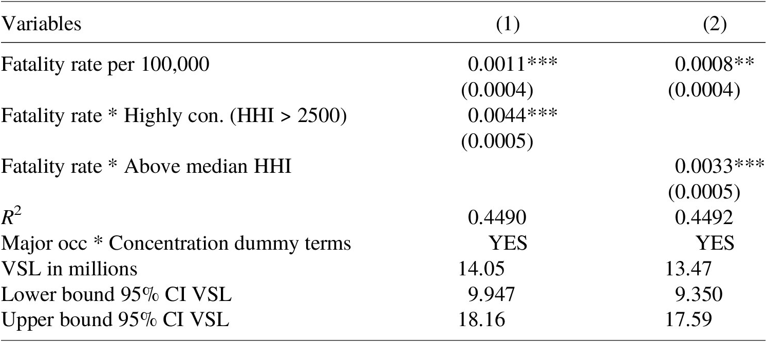
Table 5 presents the VSL yielded by an estimating equation that includes interactions between the fatality risk variable and dichotomous labor market concentration measures. Using the highly concentrated labor market variable in column 1,Footnote 22 the VSL is $14.05 million. In column 2, with the above median HHI measure, the VSL is $13.47 million, which is statistically indistinguishable from our baseline VSL. More interestingly, the coefficients on the interaction between fatality rate and the concentration dummy variable are positive, relatively large in magnitude, and statistically significant at the one percent level. This indicates that there is a substantially greater rate of compensation for marginal fatality risks for individuals in more concentrated labor markets.
Log wage regressions on fatality rates with concentration dummy variable interactions

Table 5. Long description
From top to bottom, the first column lists variables: Fatality rate per 100,000, Fatality rate times Highly con. (H HI greater than 2500), Fatality rate times Above median HH I, R squared, Major occ times Concentration dummy terms, VSL in millions, Lower bound 95 percent CI VS L, Upper bound 95 percent CI VSL. The second and third columns show results for models (1) and (2). For Fatality rate per 100,000, model (1) coefficient is 0.0011 triple asterisk, standard error 0.0004; model (2) coefficient is 0.0008 double asterisk, standard error 0.0004. For Fatality rate times Highly con. (H HI greater than 2500), model (1) coefficient is 0.0044 triple asterisk, standard error 0.0005; model (2) is blank. For Fatality rate times Above median HH I, model (1) is blank; model (2) coefficient is 0.0033 triple asterisk, standard error 0.0005. R squared is 0.4490 for model (1), 0.4492 for model (2). Major occ times Concentration dummy terms are YES for both models. VSL in millions is 14.05 for model (1), 13.47 for model (2). Lower bound 95 percent CI VSL is 9.947 for model (1), 9.350 for model (2). Upper bound 95 percent CI VSL is 18.16 for model (1), 17.59 for model (2). Statistical significance is indicated by triple asterisk for p less than 0.01, double asterisk for p less than 0.05. Standard errors are in parentheses. Notes specify controls and sample size N equals 1,329,085.
Notes: N = 1,329,085. Results reflect CPS earnings weights except for calculating the median HHI level. Standard errors clustered by state, major occupation group, and 3-digit NAICS industry in parentheses, ***p < 0.01, **p < 0.05, *p < 0.1. Each regression also includes controls for sex, race, reporting Hispanic ethnicity, education, marital status, metropolitan status, potential work experience, potential work experience squared, and whether the respondent is paid hourly, covered by a union, or works for the government. We also include 2-digit NAICS industry nonfatal injury and illness rates (with a dummy if missing in any year), state, year, and major occupation group fixed effects, a standalone concentration dummy term, and a set of interaction terms between each major occupation group and the concentration dummy (omitting the management, business, and financial occupation group interaction). To calculate the VSL, we take the sum of the coefficient on the standalone fatality rate variable and the coefficient of the interaction term multiplied by the proportion of the sample for which the concentration dummy variable equals one. The VSL standard error is estimated using the delta method on the same combination of parameters. The sample mean wage is used to calculate the VSL.
So far, we have assessed the effect of monopsony power on the VSL by allowing the fatality risk and labor market concentration variables to interact in a single estimating equation. An alternative approach is to split the main employment sample into subsamples, based on whether individuals are in “high” or “low” concentration labor markets, and then estimate separate equations for each subsample. This simplifies the VSL calculation because
$ \hat{\theta} $
 is equal to the estimated coefficient of the fatality risk parameter. Moreover, it is straightforward here to control for the independent wage effects of monopsony by setting
$ \overline{Wage} $
is equal to the estimated coefficient of the fatality risk parameter. Moreover, it is straightforward here to control for the independent wage effects of monopsony by setting
$ \overline{Wage} $
 equal to the mean wage within the high- or low-concentration subsample. This also allows our other covariates to vary depending on whether workers are in concentrated or competitive markets.
Table 6 presents results from a deeper dive into concentration’s consequences. Column 1 splits the sample according to whether the respondent works in a highly concentrated (HHI > 2500) labor market or not. The difference in the VSL estimates is marked: $28.12 million in highly concentrated labor markets compared to $8.29 million in all other labor markets. Column 2, which splits the sample based on whether respondents are in a labor market with an HHI score above or below the sample median, displays similar results, although the disparity is less dramatic. The VSL for the above-median HHI group is $20.59 million, which is smaller than the VSL for the highly concentrated subsample in column 1. The below-median HHI group VSL of $8.01 million, however, is statistically indistinguishable from the VSL for the below 2,500 HHI group.
Split sample log wage regressions on fatality rate

Table 6. Long description
From the top, the table is divided into two main sections: HHI above median and HHI below median, each with three columns labeled (1), (2), and (3). For HHI above median, fatality rate per 100,000 is 0.0049 triple asterisk, 0.0036 triple asterisk, and 0.0030 triple asterisk, with standard errors 0.0005, 0.0005, and 0.0004. Observations are 446,824, 664,528, and 664,451. R squared values are 0.4103, 0.4249, and 0.4319. VSL in millions is 28.12, 20.59, and 17.34. Lower bound 95 percent confidence interval VSL is 22.26, 15.42, and 12.29. Upper bound 95 percent confidence interval VSL is 33.97, 25.76, and 22.40. For HHI below median, fatality rate per 100,000 is 0.0014 triple asterisk, 0.0013 triple asterisk, and 0.0018 triple asterisk, with standard errors 0.0004 for all. Observations are 882,261, 664,557, and 664,634. R squared values are 0.4643, 0.4691, and 0.4633. VSL in millions is 8.292, 8.007, and 10.64. Lower bound 95 percent confidence interval VSL is 4.040, 3.404, and 6.073. Upper bound 95 percent confidence interval VSL is 12.54, 12.61, and 15.21. The table footnotes clarify that results use CPS earnings weights except for median HHI calculations, standard errors are clustered, significance levels are marked by asterisks, and regressions include multiple demographic and industry controls.
Notes: Results reflect CPS earnings weights except for calculating the various median HHI levels. Standard errors clustered by state, major occupation group, and 3-digit NAICS industry in parentheses, ***p < 0.01, **p < 0.05, *p < 0.1. Each regression also includes controls for sex, race, reporting Hispanic ethnicity, education, marital status, metropolitan status, potential work experience, potential work experience squared, and whether the respondent is paid hourly, covered by a union, or works for the government. We also include 2-digit NAICS industry nonfatal injury and illness rates (with a dummy if missing in any year) and state, year, and major occupation group fixed effects. VSL confidence intervals are computed following Kniesner et al. (Reference Kniesner, Viscusi, Woock and Ziliak2012). Each column uses the mean wage within the split sample group to calculate the VSL. The below group is inclusive of values equal to the cutoff.
It is possible that the differences in the VSL in columns 1 and 2 could partially reflect differences in the occupational composition of the high- and low-concentration subsamples. Column 3 consequently allows the relevant median HHI value used to partition the sample to vary by major occupation group. Results in column 3, where workers were only be assigned to the high- or low-concentration group based on comparisons to workers in similar jobs, show that there remain sizeable and significant differences in the implied VSLs: $17.43 million for the above-median group compared to $10.64 million for the below-median group.
Across the board, the top row of Table 6 displays VSLs that are significantly larger than the estimates in the bottom row. The results at the top of Table 6 are consistent with the existence of a steeper hedonic locus under an oligopsonistic market structure.
4.2. Hedonic wage equilibrium under monopsony
Visually, monopsony power’s impact corresponds to a steeper yet lower hedonic wage locus. In the context of Figure 1, this would correspond to Panel B. Following Viscusi and Hersch (Reference Viscusi and Hersch2001), there is likely labor market segmentation whereby workers in more concentrated occupational groups face a different market opportunities locus. The most concentrated markets have a lower wage rate, but also a different, steeper slope. The effect of employer monopsony power on the slope of the hedonic wage-risk locus appears to dominate any independent negative wage effects of reduced labor market competition in terms of its impact on the VSL.
Although workers receive lower wages in concentrated markets, they are not shortchanged in terms of compensating differentials for occupational fatality risks. A steeper hedonic locus does not imply that workers in monopsonistic markets necessarily fare better than workers in competitive markets, however. The VSL represents both the rate of compensation for additional risk and the marginal price of reduced risk. Workers in monopsonistic markets therefore (1) are paid less overall and (2) pay a greater price to move into a safer job. Moreover, in equilibrium, workers in more concentrated labor markets are in more dangerous jobs.Footnote 23
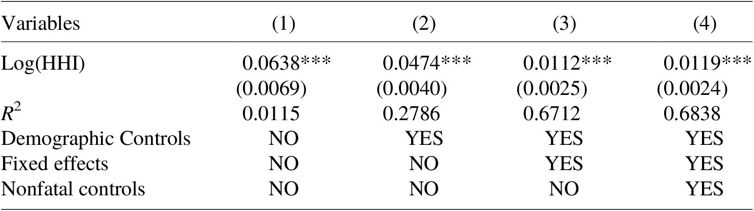
An analysis of the how job quality varies by labor market concentration levels is consistent with workers in more concentrated markets facing a greater worker fatality rate. Table 7 provides the results from a series of regressions using CFOI and CPS MORG data, where the dependent variable is the natural logarithm of one plus the fatality rate, i.e. ln(1 + rate). The explanatory variable of interest is the natural logarithm of our HHI measure. In each specification, concentration has a statistically significant and positive association with fatal job risk. A one percent increase in labor market concentration corresponds to roughly a 0.01–0.06% increase in fatality risk, depending on which covariates are included. The greater elasticity estimates of 0.05 and 0.06 are more informative since the lower estimates account for regional differences that are correlated with labor market concentration measures. Consistent with our interpretation of the equilibrium impact of our VSL findings, workers in more concentrated labor markets face greater risks.
Log fatality rate regressions on concentration

Table 7. Long description
From left to right, columns are labeled 1, 2, 3, and 4. The first row shows Log HHI coefficients: 0.0638 triple asterisk, 0.0474 triple asterisk, 0.0112 triple asterisk, and 0.0119 triple asterisk. The next row lists standard errors in parentheses: 0.0069, 0.0040, 0.0025, and 0.0024. The R squared values are 0.0115, 0.2786, 0.6712, and 0.6838. Demographic controls are NO for column 1, YES for columns 2 to 4. Fixed effects are NO for columns 1 and 2, YES for columns 3 and 4. Nonfatal controls are NO for columns 1 to 3, YES for column 4. Notes specify N equals 1,329,085, results use CPS earnings weights, the dependent variable is the natural logarithm of one plus the fatality rate, standard errors are clustered by state, major occupation group, and three-digit NAICS industry. Triple asterisk indicates p less than 0.01, double asterisk p less than 0.05, single asterisk p less than 0.1. Demographic controls include sex, race, Hispanic ethnicity, education, marital status, metropolitan status, potential work experience and its square, and indicators for hourly pay, union coverage, and government employment. Fixed effects refer to state, year, and major occupation group. Nonfatal controls refer to two-digit NAICS industry nonfatal injury and illness rate, with a dummy if missing in any year.
Notes: N = 1,329,085. Results reflect CPS earnings weights. The dependent variable is the natural logarithm of one plus the fatality rate. Standard errors clustered by state, major occupation group, and 3-digit NAICS industry in parentheses, ***p < 0.01, **p < 0.05, *p < 0.1. Demographic controls include sex, race, reporting Hispanic ethnicity, education, marital status, metropolitan status, potential work experience, potential work experience squared, and whether the respondent is paid hourly, covered by a union, or works for the government. Fixed effects refer to state, year, and major occupation group fixed effects. Nonfatal controls refer to 2-digit NAICS industry nonfatal injury and illness rate (with a dummy if missing in any year).
4.3. Robustness tests with the NLSY97
We next replicate our main results from Tables 3 and 4 using the NLSY97. An advantage of the NLSY97 is that we directly observe the county of every respondent each survey year. Additionally, we can exploit the panel data structure to control for latent individual heterogeneity in time-invariant unobservable differences such as productivity and risk preferences. We opt for a first-differences model over a fixed effects model for reasons discussed in Kniesner et al. (Reference Kniesner, Viscusi, Woock and Ziliak2012).
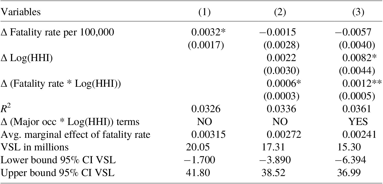
In Table 8, which is the NLSY97 analog of Table 3, we observe a similar pattern as in the CPS MORG. The baseline implied VSL without any concentration controls is $20.05 million. The 95% confidence interval of that estimate is large, ranging from -$1.7 to $41.80 million. The imprecision of the estimate is somewhat expected given the NLSY97’s considerably smaller sample size. Including both a continuous concentration measure and an interaction between concentration and fatality risk – and evaluating the VSL at
$ \hat{\theta} $
 equal to the average marginal effect of fatality risk – results in an implied VSL that is several million dollars smaller. The implied VSL that accounts for concentration ranges from $17.31 to $15.30 million, depending on whether the set of major occupation and concentration interaction terms is included.
First differences log wage regressions on fatality rates, with and without concentration interactions

Table 8. Long description
Starting from the top row, columns (1), (2), and (3) present coefficients for delta fatality rate per 100,000: 0.0032 star, negative 0.0015, negative 0.0057, with standard errors 0.0017, 0.0028, 0.0040. Delta log HHI is only in columns (2) and (3): 0.0022 and 0.0082 star, with standard errors 0.0030 and 0.0044. Delta fatality rate times log HHI interaction appears in columns (2) and (3): 0.0006 star and 0.0012 double star, with standard errors 0.0003 and 0.0005. R squared values are 0.0326, 0.0336, and 0.0361. Delta major occupation times log HHI terms are ‘NO’, ‘NO’, and ‘YES’. Average marginal effect of fatality rate is 0.00315, 0.00272, and 0.00241. VSL in millions is 20.05, 17.31, and 15.30. Lower bound 95 percent confidence interval VSL is negative 1.700, negative 3.890, and negative 6.394. Upper bound 95 percent confidence interval VSL is 41.80, 38.52, and 36.99. Statistical significance is denoted by stars, with notes indicating clustering by occupation and industry, controls for job tenure, government, union, marital, rural status, and fixed effects. Column 3 includes major occupation group interactions with log HH I.
Notes: N = 4,572. Results reflect NLSY sample weights. Standard errors clustered by major occupation group and 3-digit NAICS industry in parentheses, ***p < 0.01, **p < 0.05, *p < 0.1. Each regression also includes controls for job tenure, job tenure squared, government employee status, union status, marital status, and whether the respondent lives in a rural area. Sex, race, ethnicity, and education have insufficient intertemporal variation to be estimated with the first differences model. We also include 2-digit NAICS industry nonfatal injury and illness rates (with a dummy if missing in any year) and region, year, and major occupation group fixed effects. In column 3, we include an additional set of interaction terms between each major occupation group and log(HHI) (omitting the management, business, and financial occupation group interaction). VSL confidence intervals are computed following Kniesner et al. (Reference Kniesner, Viscusi, Woock and Ziliak2012), where the variance of the fatality risk parameter for the interaction models is estimated using the delta method. The sample mean wage is used to calculate the VSL.
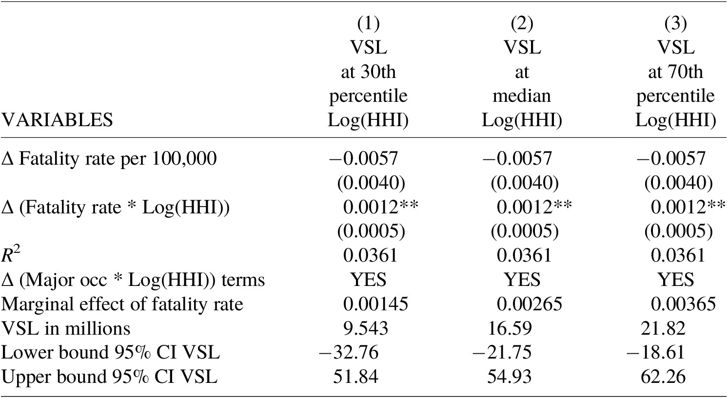
Table 9 presents the implied VSLs at different points in the log(HHI) distribution using the NLSY97 data. Like the results shown in Table 4 with the CPS MORG, moving to more concentrated labor markets increases the VSL appreciably. The observation that the NLSY97 data produce similar trends in implied VSL point estimates provides some assurance regarding our CPS estimation strategy – namely, with respect to the influence of unobserved individual heterogeneity and our inability to observe the county of every respondent in the CPS.
First differences log wage regressions on fatality rate with concentration interaction, evaluating VSL at different concentration levels

Table 9. Long description
The table has three columns labeled VSL at 30th percentile, median, and 70th percentile of concentration, each corresponding to log HHI. For the row delta fatality rate per 100,000, all columns show negative zero point zero zero five seven with standard error zero point zero zero four zero. For delta fatality rate times log HH I, all columns show zero point zero zero one two with two asterisks, standard error zero point zero zero zero five. R squared is zero point zero three six one for all columns. Delta major occupation times log HHI terms are marked yes in all columns. Marginal effect of fatality rate is zero point zero zero one four five, zero point zero zero two six five, and zero point zero zero three six five for columns one to three. VSL in millions is nine point five four three, sixteen point five nine, and twenty one point eight two. Lower bound ninety five percent confidence interval for VSL is negative thirty two point seven six, negative twenty one point seven five, and negative eighteen point six one. Upper bound ninety five percent confidence interval for VSL is fifty one point eight four, fifty four point nine three, and sixty two point two six.
Notes: N = 4,572. Results reflect NLSY sample weights. Standard errors clustered by major occupation group and 3-digit NAICS industry in parentheses, ***p < 0.01, **p < 0.05, *p < 0.1. Each regression also includes controls for job tenure, job tenure squared, government employee status, union status, marital status, and whether the respondent lives in a rural area. Sex, race, ethnicity, and education have insufficient intertemporal variation to be estimated with the first differences model. We also include 2-digit NAICS industry nonfatal injury and illness rates (with a dummy if missing in any year), region, year, and major occupation group fixed effects, a standalone log(HHI) term, and a set of interaction terms between each major occupation group and log(HHI) (omitting the management, business, and financial occupation group interaction). VSL confidence intervals are computed following Kniesner et al. (Reference Kniesner, Viscusi, Woock and Ziliak2012), where the variance of the fatality risk parameter for the interaction models is estimated using the delta method. Columns 1, 2, and 3 use the mean wage across observations in the second, third, and fourth log(HHI) quintiles, respectively, to calculate the VSL.
5. Conclusion
The research presented here examines a novel source of heterogeneity in VSL estimation: labor market power of employers. Equilibrium impacts of employer concentration are certainly of concern, and we confirm empirically that workers under oligopsony conditions are paid less, as is well documented. Moreover, we also find that the marginal price of safety, as reflected in the VSL, is greater in concentrated markets.
Our focus here has been on an issue that is also of great importance to regulatory policies for the valuation of health, safety, and environmental regulations – the effect of employer monopsony power on the estimated VSL. Regulatory benefits monetized using the VSL comprise the majority of the benefits of new government regulations (Viscusi, Reference Viscusi2018). The concern motivating our research was whether monopsony power in U.S. labor markets distorts health-enhancing regulatory decisions by leading to an underestimate of the VSL. Although workers in more concentrated markets receive lower wages and face greater fatality risks, the compensating wage differential for workplace health hazards is greater in monopsonistic markets. Policy concerns about noncompetitive forces possibly biasing VSL estimates downward, and in turn distorting policy decisions on health and safety regulations based on the VSL, are not supported by the evidence we have presented here.
The net effect of market structure and historical changes in the market structure on the average VSL is unclear. While it is possible to estimate the VSL in markets at different concentration levels, policy application of the VSL is more broadly based and does not single out markets for regulation based on their HHI index. Note that if the estimated VSL is higher in a concentrated market, that value also reflects the marginal price that firms are paying for safety. There consequently would be no market failure relative to the average societal VSL. To date, occupational health and safety regulations have been based on national evidence on risks and the average national benefits and costs of regulation. The primary implication of our examination of the heterogeneity of VSL is to alleviate the misplaced concerns that markets with a high HHI will necessarily have a low VSL and depress the average societal VSL because of the effect of monopsony on worker wage rates.
Competing interests
Our research was conducted with restricted access to Bureau of Labor Statistics (BLS) data. The views expressed here are those of the authors and do not reflect the views of the BLS. The authors declare no conflicts of interest.
A. Technical Appendix 1
We use SOC occupation to census occupation crosswalks from the U.S. Census Bureau to merge the Choi and Marinescu HHI data to the CPS MORG and NLSY97, which respectively use the 2010Footnote 24 and 2002 vintages of the census occupation coding scheme. A complication is that the crosswalks are not perfectly one-to-one. Some census occupation codes match to multiple SOC codes.Footnote 25 To handle multiple matches, we first attempted to match all census occupation codes to a six-digit SOC occupation and directly impute the Choi and Marinescu (Reference Choi and Marinescu2023) HHI score for each commuting zone. If there was no six-digit match for a census occupation code, we remove the last digit and take a weighted average of all matching five-digit SOC occupations. The weights correspond to national occupational employment estimates from the U.S. Bureau of Labor Statistics’ Occupational Employment and Wage Statistics (OEWS) program.Footnote 26 We then repeat the process at the four-digit level for all census occupation codes still missing HHI data.
Our process results in HHI scores for each 2010 census occupation (for the CPS MORG) or 2002 census occupation (for the NLSY97) and each commuting zone. We identify the commuting zone based on county information using a crosswalk also provided by Choi and Marinescu (Reference Choi and Marinescu2023). For the NLSY97, using the restricted access geocode file from the BLS, we observe the county of every respondent in each survey round. Because counties with smaller populations are not permitted to be identified in public use data, for the CPS MORG we only observe the county of residence for approximately 42% of respondents.
For the remaining CPS MORG observations with unidentified counties, we generate an aggregated state-level HHI measure for each occupation. To construct the state level measures, we start with a dataset of all counties and their annual population estimates from the U.S. Census Bureau. We then remove from that list all counties that are observed in the CPS. This is because, by definition, individuals with missing HHI data do not reside in the counties that are large enough to meet disclosure requirements. Then, we aggregate the remaining county populations into commuting zone populations because it is at that level where the Choi and Marinescu (Reference Choi and Marinescu2023) HHI data are available. If a commuting zone spans multiple states, we calculate the population within that commuting zone separately by each state. We then have a population estimate for each commuting zone in every state among the universe of unidentified counties. We also have an HHI score for each commuting zone and occupation pair. We then take a weighted average across each occupation’s HHI scores for every commuting zone in the state, where the weights equal the commuting zone’s share of the state population among the universe of unidentified counties.Footnote 27 It is worth highlighting that we do not have to use state-level aggregate HHI measures for the NLSY97 data, and so the NLSY97 analysis serves as a robustness check on the approach for the CPS MORG.
Lastly, we merge the HHI these data to the CPS MORG first using the IPUMS harmonized “occ2010” variable, and, if unsuccessful, we then attempt to use the unharmonized occupation variable. This is because there are a small number of deviations from the IPUMS harmonized “occ2010” variable and the 2010 census occupation list. To merge the HHI data to the NLSY97, we only use the census occupation code.
NLSY97 summary statistics

Table A1. Long description
The table presents summary statistics for the NLSY97 sample, with three columns: VARIABLES, Mean, and SD. From top to bottom, the variables and their values are: Hourly wage in 2022 dollars, mean 31.78, SD 16.97; HH I, mean 1,678, SD 2,168; Highly concentrated (H HI greater than 2,500) (0 or 1), mean 0.209, SD 0.407; Male (0 or 1), mean 0.549, SD 0.498; White (0 or 1), mean 0.736, SD 0.441; Black (0 or 1), mean 0.152, SD 0.359; Native American (0 or 1), mean 0.00713, SD 0.0841; Asian (0 or 1), mean 0.0239, SD 0.153; Multiracial (0 or 1), mean 0.0762, SD 0.265; Hispanic ethnicity (0 or 1), mean 0.128, SD 0.335; Tenure, mean 6.171, SD 4.981; Highest grade completed, mean 14.74, SD 3.028; Married (0 or 1), mean 0.555, SD 0.497; Rural (0 or 1), mean 0.199, SD 0.399; Government worker (0 or 1), mean 0.187, SD 0.390; Union (0 or 1), mean 0.166, SD 0.372; Injury and illness rate per 100,000, mean 954.6, SD 534.3; Missing injury and illness rate (0 or 1), mean 0.0121, SD 0.109; NC A, mean 0.157, SD 0.363. The sample size is 9,318, and results reflect NLSY sample weights. For missing injury and illness rate data, the rate is set to zero and a dummy variable is included.
Notes: N = 9,318. NLSY97 summary statistics from Rounds 18, 19, and 20. Results reflect NLSY sample weights. For the small number of observations missing injury and illness rate data, we set the injury and illness rate equal to zero and include a separate dummy variable.




 Open access

