


1. Introduction
The mass balance (or mass budget) of a glacier, ∆M, is defined as the change in glacier mass over a defined period of time (Cogley and others, Reference Cogley2011) and thus is a measure of glacier health and an important indicator of climate change (Oerlemans, Reference Oerlemans2001; Bojinski and others, Reference Bojinski, Verstraete, Peterson, Richter, Simmons and Zemp2014). Globally, glaciers and ice sheets are losing mass at an increasing pace (Mouginot and others, Reference Mouginot2019; Schröder and others, Reference Schröder, Horwath, Dietrich, Helm, Van Den Broeke and Ligtenberg2019; Zemp and others, Reference Zemp2019; Hugonnet and others, Reference Hugonnet2021; Otosaka and others, Reference Otosaka2023; The GlaMBIE Team, 2025), which directly affects, among other, global sea level, streamflow quantities and quality, glacial hazards, landscape evolution, terrestrial and marine ecosystems and human systems (Hock and others, Reference Hock, Pörtner DCR, Masson-Delmotte, Zhai, Tignor, Poloczanska, Mintenbeck, Alegría, Nicolai, Okem, Petzold, Rama and Weyer2019). Hence, it is important to accurately determine ongoing glacier mass changes at local to global scales.
Several methods have been developed to determine glacier mass balance from direct observations, and in particular major advances in satellite technology in the last couple of decades have revolutionized our ability to assess and monitor glacier changes on large scales (Berthier and others, Reference Berthier2023). Methods can broadly be categorized into three principal approaches: the glaciological or direct method, which relies on in situ glacier observations of ablation stakes and snow pits; the geodetic method, which, as historically defined in glaciology, relies on differencing glacier elevations at different times; and the gravimetric method, which derives mass changes from satellite-derived gravity data (Cogley and others, Reference Cogley2011). The latter two methods have been used for both glaciers and ice sheets, whereas the glaciological method is inadequate for deriving ice-sheet-wide balances.
Each method possesses unique strengths and weaknesses, alongside varying limitations contingent upon spatial domain and temporal resolution. However, even when accurate, estimates derived from different methods or sources are often challenging to compare due to various factors. These include instances where reported balances may omit certain components due to methodological constraints, discrepancies in the time spans and precise spatial domains considered, or the reporting of mass balances in different units without sufficient information for conversion. These challenges impede the synthesis of regional to global mass-change estimates, which is critical for accurately quantifying the components of sea-level change. This is particularly significant within the context of international assessments, such as the Intergovernmental Panel on Climate Change (IPCC), which frequently combine estimates from various studies and methods (e.g. Oppenheimer and others, Reference Oppenheimer, Pörtner DCR, Masson-Delmotte, Zhai, Tignor, Poloczanska, Mintenbeck, Alegría, Nicolai, Okem, Petzold, Rama and Weyer2019; Masson-Delmotte and others, Reference Masson-Delmotte2021).
In light of these challenges, the purpose of this paper is to (a) review the main characteristics, including their respective strengths and weaknesses, of various mass-balance measuring methods in the context of comparing and synthesizing reported data; (b) identify key challenges hindering the direct comparison of mass-balance estimates obtained from different methods and sources; and (c) develop and outline best practices for deriving and reporting mass balances to enhance comparability and streamline the integration of regional mass balances from diverse sources (e.g. for inclusion in global estimates). We focus on the difficulties encountered when comparing or combining mass balances derived from various methods into larger-scale estimates, rather than providing an exhaustive account of the inherent uncertainties associated with each individual method. Although our primary emphasis is on glaciers outside the ice sheets, most of the issues and recommendations discussed herein are also pertinent to observations of the ice sheets.
2. Measuring mass balance
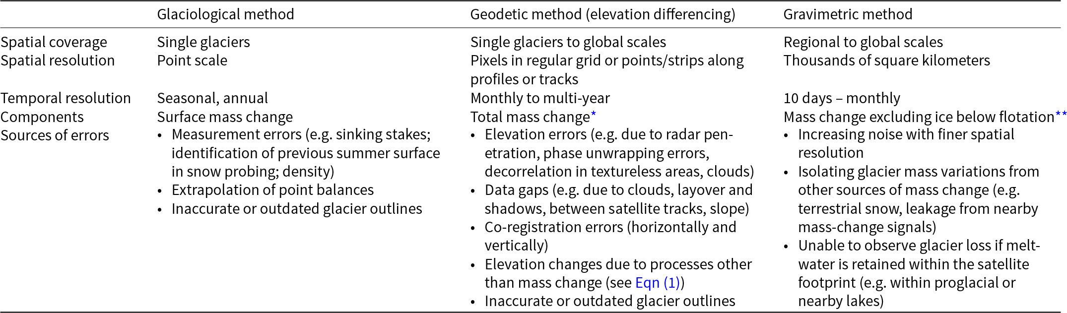
We provide a brief overview of the three principal mass-balance methods mentioned earlier, but refer to the literature and other review papers for further details (Østrem and Brugman, Reference Østrem and Brugman1991; Braithwaite, Reference Braithwaite2002; Cogley and others, Reference Cogley and Anderson2005, Reference Cogley2011; Bamber and Rivera, Reference Bamber and Rivera2007; Berthier and others, Reference Berthier2023). Table 1 summarizes typical characteristics of these methods. For mass-balance purposes, the glacier comprises only ice, snow and firn. Sediments and supra-, sub- or englacial water are not part of the glacier and therefore not included in glacier mass balance (Cogley and others, Reference Cogley2011), although, in practice, distinguishing these components is often not straightforward in observations. While mass balances can be reported over any domain of a glacier and any time period, it is common practice to compute them over entire glaciers (or glacier regions) and over seasonal, annual and multi-annual time scales, although recent methodological advances (e.g. gravimetry, altimetry) have allowed increasingly finer temporal resolution (see Sections 2.2 and 2.3).
Summary of typical characteristics, error and uncertainty sources of the three principal glacier mass-balance methods. ‘Spatial resolution’ refers to the scale of the actual observations. ‘Components’ refer to the components of mass balance captured by the method.

* Mass change of deglaciated or newly glaciated portions below the water surface of grounded tidewater or lake-terminating glacier is not included if DEM elevations used for differencing refer to the water surface rather than the underwater bed. If the ice is floating, only ∼10% of the total thickness change will be measured (see Section 3.2).
** If floating ice is replaced by water, there is no net mass change and therefore no signal in GRACE.
In case of grounded ice, the sea-level contribution captured by GRACE is proportional to the difference between the density of water replacing the melted ice volume (roughly 1000 kg m−3 depending on salinity) and the density of the grounded ice (roughly 900 kg m−3), divided by the former, i.e. approximately 10% of actual mass change.
2.1. Glaciological method
The direct or glaciological method is the oldest approach (Østrem and Brugman, Reference Østrem and Brugman1991) and the only one based exclusively on in situ measurements performed directly on the glacier. While various implementations exist, the method involves measuring the change in elevation of the glacier surface relative to a reference marker close to the surface at individual locations across the glacier (usually derived from measuring the height above the surface of a stake drilled into the glacier). For summer or annual balances, the reference marker is typically the top of an ablation stake, and for winter balances based on snow probing, it is the last summer surface. Note that the reference marker is not fixed in elevation above sea level due to the vertical ice motion caused, for example, by ice flow or subglacial erosion.
The measurements are subsequently converted into mass changes based on density observations in snow pits or suitable assumptions to determine the mass added or removed at the surface. The point balances are then extrapolated across the entire glacier, assuming elevation-dependent (i.e. hypsometric) functions (e.g. Wagnon and others, Reference Wagnon2013; Sold and others, Reference Sold2016) or other geospatial interpolation techniques (e.g. Cogley and Adams, Reference Cogley and Adams1998; Hock and Jensen, Reference Hock and Jensen1999) to yield the glacier-wide balance. Instead of purely statistical methods, process-based models constrained with all seasonal measurements have also been used to infer glacier-wide mass balance from point observations (Huss and others, Reference Huss2021). Ideally, the glacier area is updated annually, but in practice updates are usually less frequent because up-to-date glacier outlines are not always available.
The derived mass balances only capture the surface mass balance, i.e. the sum of accumulation and ablation at the glacier surface (Cogley and others, Reference Cogley2011). Where relevant, mass changes within the glacier (e.g. internal accumulation) or basal mass changes (Andreassen and others, Reference Andreassen, Elvehøy, Kjøllmoen and Engeset2016; Jóhannesson and others, Reference Jóhannesson2020; Hösli and others, Reference Hösli2025), as well as frontal ablation (Kochtitzky and others, Reference Kochtitzky2022) at marine- or lake-terminating glaciers (mostly calving and submarine melt), need to be determined separately and added to the surface balance to obtain a glacier’s total mass balance.
The temporal resolution is determined by the frequency of field visits, typically once or twice a year to allow the calculation of annual or seasonal (winter, summer) balances, respectively, although some glaciers in the tropics have been monitored every month (Rabatel and others, Reference Rabatel2013), and daily mass-balance monitoring using automated systems is increasingly deployed (Landmann and others, Reference Landmann, Künsch, Huss, Ogier, Kalisch and Farinotti2021).
Due to logistical challenges, the glaciological method is primarily used for small and accessible glaciers. Globally, 75% of the glaciers monitored by this method have an area of less than 10 km2, and 80% are situated between the polar circles (66° N to 66° S) (WGMS, 2024).
2.2. Geodetic method (surface elevation differencing)
2.2.1. Overview
Any method that derives a glacier mass balance from volume change computed from repeated mapping of surface elevations over the (changing) glacier surface is referred to as the geodetic method (Cogley and others, Reference Cogley2011). Note that this definition, common in glaciology, differs from the one used in geodesy, where the term refers to a suite of techniques to measure (changes in) the Earth’s geometric shape, orientation in space and gravity field using both space-based and terrestrial observations (Torge and Müller, Reference Torge and Müller2012), and thus includes both surface elevation-differencing methods and the gravimetric method.
Glacier surface elevation data were initially derived from terrestrial (i.e. land survey) or aerial photogrammetry (e.g. Kick, Reference Kick1966; Finsterwalder and Rentsch, Reference Finsterwalder and Rentsch1976). Since the 1990s, particularly after the year 2000, the primary sources of elevation data have shifted to satellite data derived from radar or laser altimetry, synthetic aperture radar and optical imagery (Berthier and others, Reference Berthier2023 and references therein), or airborne laser altimetry (e.g. Echelmeyer and others, Reference Echelmeyer1996). Recently, declassified analog ‘spy imagery’ — such as data from the Corona KH-1 to KH-6 and Hexagon KH-9 series — has enabled the determination of mass balances dating back to the 1970s (Maurer and others, Reference Maurer, Rupper and Schaefer2016; Dehecq and others, Reference Dehecq2020). Contemporary advances in photogrammetry and structure from motion techniques have opened new opportunities for high-resolution mapping of glacier surface elevations, extending back to the early 20th century (Geyman and others, Reference Geyman, van Pelt, Maloof, Aas HF and Kohler2022; Mannerfelt and others, Reference Mannerfelt2022).
Surface elevation changes are either determined from differencing (a) two or more digital elevation models (DEMs) or (b) elevations measured along satellite or airplane tracks, typically based on radar or lidar altimetry. To deal with voids and unmapped areas in the former approach, the elevation change fields are usually interpolated rather than the underlying DEMs (Pieczonka and Bolch, Reference Pieczonka and Bolch2015; McNabb and others, Reference McNabb, Nuth, Kääb and Girod2019; Seehaus and others, Reference Seehaus, Morgenshtern, Hübner, Bänsch and Braun2020). Since sampled far more sparsely, elevation change measurements along satellite or airplane tracks need to be extrapolated to the entire glacier surface, typically done as a function of elevation (i.e. hypsometric approach) or other co-variables (Arendt and others, Reference Arendt, Echelmeyer, Harrison, Lingle and Valentine2002; Moholdt and others, Reference Moholdt, Nuth, Hagen and Kohler2010; Kääb and others, Reference Kääb, Berthier, Nuth, Gardelle and Arnaud2012; O’Neel and others, Reference O’Neel2019; Fan and others, Reference Fan, Ke, Zhou, Shen, Yu and Lhakpa2023).
Mass balances derived from DEM differencing have typically been determined over multi-year or multi-decadal periods (e.g. Belart and others, Reference Belart2020; McDonnell and others, Reference McDonnell, Rupper and Forster2022). Results for individual glaciers have been used to correct time series of annual glaciological mass balances for systematic errors, assuming the longer-term balances to be more robust (e.g. Zemp and others, Reference Zemp2013; Andreassen and others, Reference Andreassen, Elvehøy, Kjøllmoen and Engeset2016; Wagnon and others, Reference Wagnon2021). Recent studies have also estimated mean mass-balance rates over multi-year periods from temporal regressions of multi-survey elevations of each DEM pixel individually obtained at varying points in time (e.g. Berthier and others, Reference Berthier, Cabot, Vincent and Six2016; Dussaillant and others, Reference Dussaillant2019; Shean and others, Reference Shean, Bhushan, Montesano, Rounce, Arendt and Osmanoglu2020; Hugonnet and others, Reference Hugonnet2021; Minowa and others, Reference Minowa, Schaefer, Sugiyama, Sakakibara and Skvarca2021; Bernat and others, Reference Bernat2023) as initially pioneered by Nuimura and others (Reference Nuimura, Fujita, Yamaguchi and Sharma2012) and Willis and others (Reference Willis, Melkonian, Pritchard and Ramage2012).
Mass balances based on satellite altimetry have also been reported with higher temporal resolution (e.g. monthly), both over ice sheets (e.g. Lai and Wang, Reference Lai and Wang2021; Nilsson and others, Reference Nilsson, Gardner and Paolo2021; Scanlan and others, Reference Scanlan, Rutishauser, Hansen and Simonsen2025) and for glaciers outside the ice sheets (Jakob and Gourmelen, Reference Jakob and Gourmelen2023). This enhanced resolution is made possible by the frequent repeat orbital cycles of the available satellites.
2.2.2. Components of elevation change
It is important to recognize that glacier elevation change can be influenced by processes other than mass change. Total elevation change Δh at any point on a glacier is given by:
 \begin{equation}\Delta h = \,\Delta {h_b} + \Delta {h_{flux}} + \Delta {h_{dens}} + \Delta {h_{bed}} + \Delta {h_{water}}\end{equation}
where elevation changes Δh x are due to different processes: b is the climatic-basal mass balance, i.e. the mass change at or near the surface mainly driven by climate, and at the glacier bed, but not due to ice flow (Cogley and others, Reference Cogley2011), flux is the flux divergence caused by ice flow, dens refers to densification (compaction) of snow and firn, bed refers to changes in bed elevation caused by vertical ground movement due to tectonics, isostatic movements or geomorphological processes (e.g. erosion) and water refers to changes in subglacial water storage.
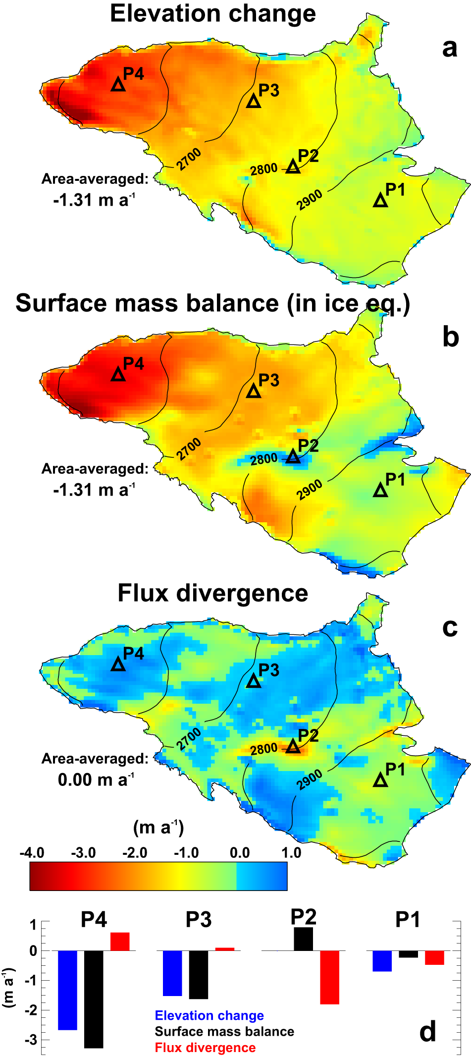
Only the first two terms reflect glacier mass change (Fig. 1). Consequently, elevation changes can occur without any change in mass due to the latter three terms. For example, surface elevation can change due to densification without any change in mass (e.g. Schaffer and others, Reference Schaffer, Copland, Zdanowicz, Burgess and Nilsson2020; Ochwat and others, Reference Ochwat, Marshall, Moorman, Criscitiello and Copland2021). While Δh dens can be substantial in the firn area, especially over shorter (e.g. seasonal) time periods (Reeh, Reference Reeh2008), the latter two terms (Δhbed and Δhwater) are often negligible but can be significant locally. For example, subglacial erosion rates of almost 4 m a−1 were found locally on Taku Glacier, Alaska (Motyka and others, Reference Motyka, Truffer, Kuriger and Bucki2006). Isostatic rebound can be important when considering longer time periods (e.g. present-day uplift rates of up to 3 and 4 cm a−1 have been found in southeast Alaska (Hu and Freymueller, Reference Hu and Freymueller2019) and Patagonia (Dietrich and others, Reference Dietrich, Ivins, Casassa, Lange, Wendt and Fritsche2010), respectively). Additionally, a temporary uplift of 0.6 m was observed at the onset of the melt season at Unteraargletscher, Switzerland, caused by water storage at the bed (Iken and others, Reference Iken, Röthlisberger, Flotron and Haeberli1983). Similar uplifts, varying between 0.20 and 0.90 m over the winter/spring season were found at Argentière Glacier, and attributed largely to water-filled cavities (Vincent and others, Reference Vincent2022).
Illustration of components of elevation change exemplified with spatially distributed data from Silvrettagletscher, Switzerland, over the period 2012–20. (a) Surface elevation change Δh based on DEM differencing (GLAMOS, 2024). (b) Surface mass balance (derived from process-based model constrained by annual in situ measurements at 17 stakes, and then converted into ice-/firn-equivalent elevation changes) (Huss and others, Reference Huss, Dhulst and Bauder2015). (c) Emergence (positive) and submergence (negative values) velocity due to flux divergence computed from the difference between (a) and (b). Surface mass balance is expressed in ice equivalent to facilitate comparison with the other components. Elevation changes due to other components than surface mass change and ice flow (Eqn (1)) are assumed negligible. In panel (d), all components are extracted from four point locations with direct measurements. The glacier is strongly out of balance as indicated by negative surface mass balances across almost the entire glacier.

If the sum of the last three terms is zero, this geodetic method measures total mass balance at single points/pixels, since, unlike the glaciological method, it captures the flux divergence. The primary distinction is that elevations are given in relation to a geodetic datum or other standard reference (geodetic method) instead of being relative to a local reference marker situated near the surface (glaciological method, see Section 2.1). However, while it can be a major component at the point scale, conveniently, Δh flux cancels out when integrated over an entire (land-terminating) glacier, thus allowing the calculation of glacier-wide mass balance from elevation change (or the glaciological method) without the need to account for ice flow.
2.2.3. Converting elevation change to mass change
Elevation change at any point on the glacier is converted into specific mass change Δm (kg m−2) by:
 \begin{equation}\Delta m = f\,\Delta h\end{equation}
where f is a conversion factor (kg m−3). Earlier studies tended to use a value equivalent to the approximate density of glacier ice (900 kg m−3, e.g. Arendt and others (Reference Arendt, Echelmeyer, Harrison, Lingle and Valentine2002)) to convert glacier-averaged Δh to mass change, thus assuming that the density structure of the firn area did not change over time (Bader, Reference Bader1954). Many recent studies have applied a spatially constant factor of 850 ± 60 kg m−3 (e.g. Kienholz and others, Reference Kienholz, Hock, Truffer, Arendt and Arko2016; Braun and others, Reference Braun2019; Yang and others, Reference Yang, Hock, Kang, Shangguan and Guo2020; Tepes and others, Reference Tepes, Gourmelen, Nienow, Tsamados, Shepherd and Weissgerber2021; Sommer and others, Reference Sommer, Seehaus, Glazovsky and Braun2022), as suggested by Huss (Reference Huss2013) for time periods exceeding 5 years, thus accounting for generally decreasing firn volumes as glaciers lose mass. Some studies used spatially variable conversion factors, such as lower values in the accumulation area than the ablation area, to account for density differences between glacier zones (e.g. Kääb and others, Reference Kääb, Berthier, Nuth, Gardelle and Arnaud2012; Foresta and others, Reference Foresta2018; Malz and others, Reference Malz, Meier, Casassa, Jaña, Skvarca and Braun2018). Stevens and others (Reference Stevens, Sass, Florentine, McNeil, Baker and Bollen2024) used firn measurements to constrain the conversion factor on a valley glacier, while firn densification models are increasingly employed on the ice sheets (e.g. Gardner and others, Reference Gardner, Schlegel and Larour2023; Kappelsberger and others, Reference Kappelsberger2024; Sanchez Lofficial and others, Reference Sanchez Lofficial2025) but also ice caps (Schaffer and others, Reference Schaffer, Copland, Zdanowicz, Burgess and Nilsson2020) to correct the observed surface elevation changes and then multiply them by the density of ice. Thus, these studies effectively adopt a spatially varying conversion factor f for observed Δh (Eqn (2)).
However, since elevation change can occur without any change in mass, or vice versa, mass change without any elevation change, f in Eqn (2) can range from −infinity to +infinity. Thus, it may deviate substantially from the average density of the actual material added to or removed from the glacier. The conversion of elevation change to mass change is especially prone to large uncertainties over short time frames, such as seasonal scales, during which changes in near-surface density structure of the glacier tend to be particularly pronounced (Pelto and others, Reference Pelto, Menounos and Marshall2019; Huss, Reference Huss2013).
2.3. Gravimetric method
The gravimetric method determines mass changes from repeat measurements of the variations in the Earth’s gravity field. Since the gravitational force depends on mass, any changes in the Earth’s gravity field are indicative of mass changes. The method has gained traction during the Gravity Recovery and Climate Experiment (GRACE) satellite mission (2002–17) and its follow-on mission launched in 2018 (GRACE-FO) allowing for global-scale glacier and ice-sheet mass-change estimation. Both missions include polar-orbiting twin satellites separated by approximately 220 km. The precise distance between the satellites varies as the gravitational pull on each satellite varies as the local gravity field changes along the orbit. By continuously measuring the changes in the distance between the two satellites, the Earth’s gravity field and its temporal changes can be mapped, which on short time scales is predominantly related to redistribution of water on its surface (Tapley and others, Reference Tapley2019). The method yields a direct measure of mass changes, thus circumventing the need for a density correction; however, derived glacier mass changes depend on the accuracy of models to remove the mass-change signal due to atmospheric and oceanic (Dobslaw and others, Reference Dobslaw2017), spheric (e.g. ground water storage; Rodell and others, Reference Rodell, Velicogna and Famiglietti2009) and lithospheric mass variations (e.g. due to glacial isostatic adjustments; Sørensen and others, Reference Sørensen2017). Most studies are based on monthly averages with mass balances reported with respect to the middle of the month, although a few studies are based on shorter intervals, such as 10 day averages (Fu and Freymueller, Reference Fu and Freymueller2012; Arendt and others, Reference Arendt2013; Luthcke and others, Reference Luthcke, Sabaka, Loomis, Arendt, McCarthy and Camp2013). The spatial resolution is typically in the order of 250–350 km with the finest resolution studies reaching about 150 km (Loomis and others, Reference Loomis, Felikson, Sabaka and Medley2021; Willen and others, Reference Willen, Wouters, Broerse, Buchta and Helm2025).
3. Challenges in comparing published glacier mass balances
Comparing reported mass balances derived from different methods and studies can pose significant challenges, which can be broadly categorized into four main areas: (1) inconsistent reporting and lack of relevant information, (2) differences in the mass-balance components included, (3) differences in the time span considered and (4) differences in the spatial domain of the reported mass balance.
3.1. Units and mass-balance reporting
3.1.1. Units
Depending on the study’s objectives, spatial scale and the mass-balance method employed, mass balances are reported in different units across different studies, complicating direct comparisons. Glaciological mass balances have traditionally been reported in specific units, i.e. mass change per unit area expressed in kg m−2 or m water equivalent (w.e.), where 1000 kg m−2 is equivalent to 1 m w.e. with a density of water of 1000 kg m−3. In contrast, elevation change or gravimetrically derived balances are often reported in Gigatons (1 Gt = 1012 kg = 1 km3 water) and sometimes as volume change (km3 ice equivalent).
The use of specific units facilitates climatological interpretations of glaciers of varying sizes, while mass units are more appropriate for hydrological or oceanographic purposes where total water volumes are crucial. Global or regional-scale estimates are often also reported in sea-level equivalent (SLE) with typical units in meter or mm SLE, referring to the change in mean global sea-level that results from the addition or removal of water due to glacier mass change. However, mass changes reported in unit m SLE may also differ in the way they were calculated. Many studies simply divide the mass of water lost or gained by the glaciers by the product of the density of freshwater and a fixed ocean area (e.g. Gardner and others, Reference Gardner2013; Zemp and others, Reference Zemp2019; Hock and others, 2019; Marzeion and others, Reference Marzeion2020), thus neglecting any other processes that would affect mean global and regional sea level, such as shoreline migration or changes in bathymetry (Cogley and others, Reference Cogley2011). Some global-scale studies (e.g. Huss and Hock, Reference Huss and Hock2015; Rounce and others, Reference Rounce2023; Zekollari and others, Reference Zekollari2025) or regional assessments (e.g. Arendt and others, Reference Arendt2006; Braun and others, Reference Braun2019; Kochtitzky and others, Reference Kochtitzky2022; Zhang and others, Reference Zhang2023) account for ice below sea level of grounded tidewater glaciers that is already displacing ocean water (roughly 15% of all glacier ice outside the ice sheets; Farinotti and others, Reference Farinotti2019), and thus only negligibly contributing to sea level.
Although converting reported mass balances from various studies into comparable units may seem straightforward in theory, it often becomes challenging in practice due to the lack of essential information reported in the literature. For example, to allow conversion of specific units into mass units, the applied glacier area is needed. Similarly, converting SLE values into other units and vice versa, ocean area and water density values are needed, but values have varied across studies (Hock and others, Reference Hock, Maussion, Marzeion and Nowicki2023).
3.1.2. Reporting of balances from different methods
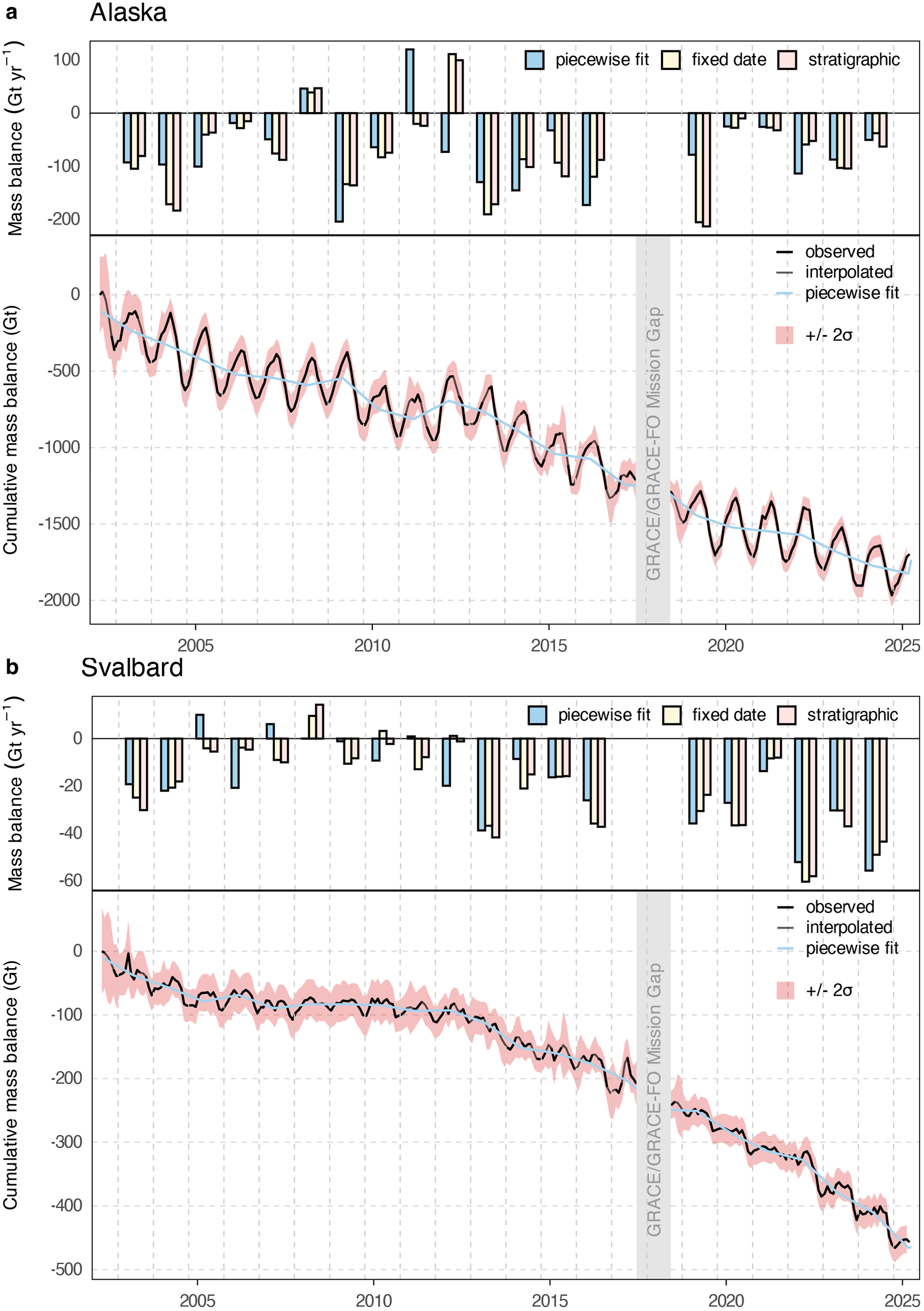
In addition, regardless of the unit, mass balances are often presented in particular ways depending on the method, further complicating direct comparison. Glaciological balances are generally presented as annual (and if available also seasonal) balances; geodetic balances based on DEM-differencing are most often expressed as average rates over multi-year periods. In contrast, altimetry and GRACE-derived estimates are typically shown as cumulative mass change, i.e. the mass change as a function of time relative to the mass at some earlier time or a mean over a given period (Fig. 2). Hence, comparing results to mass balances derived from the other methods may necessitate transforming the data into comparable quantities.
Annual mass balances (upper panels) extracted from cumulative mass anomalies (lower panels) from GRACE and GRACE-FO for the period April 2022–March 2025 for (a) Alaska and (b) Svalbard. Observational gaps (gray) are filled using spline interpolation. The light red band shows the two-sigma uncertainty in the monthly observations. Specific annual balances in the bar charts are computed in a fixed-date time system using mass-balance years of 1 September–30 August of the following year (‘fixed date’), in the stratigraphic time system (balance between consecutive annual mass minima; ‘stratigraphic’) and using annual linear trends based on a piecewise fit with break points on 1 March of each year (‘piecewise fit’) (Sasgen and others, Reference Sasgen2022). Date labels refer to 1 January, while vertical grid lines mark the start of the fixed-date mass-balance year (1 September). The GRACE data were processed following Wouters and others (Reference Wouters, Gardner and Moholdt2019).

Various approaches have been employed to compute mass-balance rates from cumulative GRACE time series: For example, Arendt and others (Reference Arendt, Luthcke and Hock2009) computed 10-day mass balances from the differences of sequential 10-day cumulative balances for glaciers in Alaska over 4 years (whereby each 10-day data point represented a time-averaged mass value). Annual mass balances are typically extracted by differencing the monthly observations of two consecutive years, which can be a fixed month for every year (fixed-date system, see Section 3.3) or variable months from year to year. The latter approach was used in Luthcke and others (Reference Luthcke, Arendt, Rowlands, McCarthy and Larsen2008), who differenced consecutive yearly (monthly mean) minima, thus presenting annual balances in the stratigraphic time system (Cogley and others, Reference Cogley2011). Wouters and others (Reference Wouters, Gardner and Moholdt2019) computed annual balances for all major glacier regions outside the ice sheets as the differences between the cumulative mass-balance values for 30 September and 1 October of the previous year (shifted by half a year in the Southern Hemisphere), interpolating the exact day values through spline interpolation of monthly values. Box and others (Reference Box2018) provided annual mass-balance estimates for Arctic regions based on differencing successive September mass anomalies. Because of the relatively high noise level in monthly GRACE observations, differencing individual months comes at the cost of relatively high uncertainties in the yearly mass balances. In a study focusing on Arctic glaciers, Sasgen and others (Reference Sasgen2022) derived annual mass balances based on a piecewise linear fit with break points on 1 March of each year. The effect of different methods to derive annual balances from continuous GRACE time series is illustrated for Alaska, a region with pronounced seasonal cycles, and Svalbard, which exhibits less distinct mass-balance cycles (Fig. 2). In both cases, annual balances vary significantly depending on the chosen time system or method used.
Multi-year mass balances are usually computed from linear regression of the cumulative mass anomaly curve (Ciracì and others, Reference Ciracì, Velicogna and Swenson2020), where a trend is co-estimated together with annual, semi-annual and sometimes higher-frequency harmonics. This reduces the sensitivity of the mass-balance estimates to the usage of non-integer years, at least for sufficiently long observational records. Some studies use weighted linear regression, where the weights are based on the estimated noise in the data, to account for variable data quality (e.g. Wouters and others, Reference Wouters, Gardner and Moholdt2019). For example, the quality of the GRACE data is dependent on the orbital configuration of the satellites and instrument performance (e.g. one accelerometer in one of the GRACE satellites needed to correct for non-gravitational forces affecting the satellite orbit stopped functioning in September 2016, degrading the data quality (Bandikova and others, Reference Bandikova, McCullough, Kruizinga, Save and Christophe2019)).
3.2. Mass-balance components
Not all methods measure all components of total mass balance, which include accumulation and ablation at the surface, inside and at the base as well as mass losses at any near-vertical margin of a glacier such as a calving front (Cogley and others, Reference Cogley2011):
 \begin{equation}\Delta M = {B_{{\text{sfc}}}} + {B_{\text{i}}} + {B_{\text{b}}} + {A_{\text{f}}}\end{equation}
where B sfc is the surface mass balance (often dominated by snowfall and melt), B i is the internal balance (e.g. internal accumulation due to refreezing), B b is the basal balance and A f is frontal ablation (mass loss at near-vertical glacier margins through calving, subaerial melting and sublimation, and subaqueous frontal melting). This formulation distinguishes the different locations of a glacier where mass changes can occur rather than considering the physical processes, but it is convenient from a measurement point of view.
The glaciological method only captures B sfc. For many of the glaciers monitored this way, this limitation is not an issue, since the method is mostly applied to land-terminating glaciers where other components tend to be negligible. However, B b can be a significant component in active volcanic areas (Jóhannesson and others, Reference Jóhannesson2020). Internal accumulation and internal ablation (both contributing to B i) have been found important in high-latitude regions (Trabant and Mayo, Reference Trabant and Mayo1985; Reijmer and Hock, Reference Reijmer and Hock2008) and on some maritime high-precipitation glaciers, respectively (Alexander and others, Reference Alexander, Shulmeister and Davies2011; Andreassen and others, Reference Andreassen, Elvehøy, Kjøllmoen and Engeset2016). A f, a significant component at tidewater and lake-terminating glaciers, can be derived from estimates of ice flux across a fixed flux-gate some distance from the terminus as a function of surface velocities and ice thickness, changes in front position, and estimates of the climatic-basal mass balance of the glacier portion below the fluxgate (McNabb and others, Reference McNabb, Hock and Huss2015; Deschamps-Berger and others, Reference Deschamps-Berger, Nuth, van Pelt, Berthier, Kohler and Altena2019; Kochtitzky and others, Reference Kochtitzky2022).
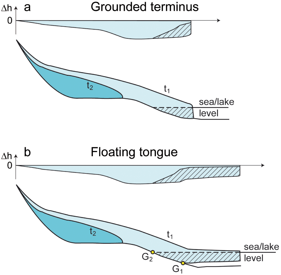
In principle, if elevation changes not caused by mass changes (Eqn (1)) can be accounted for and appropriate elevation-to-mass conversion factors (Eqn (2)) are applied, the geodetic (surface elevation differencing) method encompasses all mass-balance components, albeit without the ability to distinguish individual components. However, a significant complication may arise for tidewater or lake-terminating glaciers that experience terminus retreat or advance (Fig. 3). In practice, DEMs provide the elevation of the ocean or lake surface for the deglaciated ocean or lake area after a glacier retreat or before an advance. Therefore, for grounded glaciers, the method fails to account for any mass changes occurring beneath the water level in the deglaciated or newly glaciated terrain, capturing only the changes above the water surface (Fig. 3a; Goelzer and others, Reference Goelzer, Coulon, Pattyn, De Boer and Van De Wal2020). To address this issue, the underwater component must be assessed independently, or the DEMs should be pre-processed by substituting surface elevations with underwater ocean or lake-floor elevation data.
Illustration of the effect of the presence of subaqueous ice on elevation differencing for (a) a grounded glacier and (b) a glacier with a floating tongue that retreated onto land. The longitudinal profile before (t 1) and after the retreat (t 2), and the corresponding elevation change Δh based on DEM data and the actual ice thickness change, are shown for each case. The hatched areas correspond to the glacier thickness losses not captured directly by surface elevation differencing. In the case of a floating tongue (panel b), total ice thickness change can be derived from surface elevation measurements since measured Δh over the floating tongue is approximately 1/10th of the total ice thickness change due to hydrostatic equilibrium. As the grounding line shifts with the retreat of the glacier, the ratio transitions from 0.1 to 1 between points G 1 and G 2 (the initial and the highest possible location of the grounding line, respectively). However, the precise ratio at each specific point can no longer be accurately determined retrospectively, adding uncertainty to the ice thickness change estimate in this zone.

For floating tongues, this is less of an issue in principle since they are in hydrostatic equilibrium (Fig. 3b). Thus, the change in total ice thickness (which includes submerged ice) can be approximated by multiplying the elevation change relative to the water level by a factor of 10 (Trüssel and others, Reference Trüssel, Motyka, Truffer and Larsen2013). This factor accounts for approximately the density difference between ice and water. Nevertheless, accurate handling of the terminus regions of marine- or lake-terminating glaciers necessitates understanding whether and which parts of the terminus region were grounded or floating, and the situation becomes more intricate if the grounding line moved during the period under consideration. Furthermore, floating ice near the grounding line is not in hydrostatic equilibrium, introducing further errors. In addition, accurate outlines of the marine- or lake-terminating terminus region matching the elevation data are needed but not always available.
Incorporating underwater mass changes is important when the total glacier mass change is the focal variable, such as in evaluating the impact of freshwater influx into the ocean. Kochtitzky and others (Reference Kochtitzky2022) estimated that the total mass loss of all glaciers in the Northern Hemisphere outside the Greenland ice sheet during 2000–2020 would be underestimated by 2–4% if this component were not accounted for. However, if the focus is on the glacier contribution to sea-level change, it is important to note that for both grounded and floating glacier tongues, by far most of the underwater change (∼90%) does not contribute to sea-level change. This is because the submerged portion of the ice already displaces ocean water. Disregarding this component facilitates direct comparison with GRACE-derived mass balances, which exclude below-flotation mass changes. Therefore, the relevance of omitting this component, considering current DEM availability, hinges on the specific purpose of the mass-change calculations.
3.3. Time period and time systems
Mass budgets outside the tropics are typically characterized by net mass gain over winter and net mass loss in summer, thus exhibiting distinct cyclic behavior. Therefore, differences in the exact time span that a balance refers to can be a significant source of uncertainty when comparing annual values or multi-year average rates from different studies and methods. Mass-balance rates over longer periods of time (typically reported in mass change per year) are ideally derived over time spans of an integer number of years. However, in practice, this is often not the case due to observational constraints.
For global assessments, further complications can arise when balances are reported over mass-balance years (the roughly annual period between consecutive mass minima), since mass-balance years are shifted by 6 months in the Southern Hemisphere compared to the Northern Hemisphere, and the exact time span also can vary as a function of latitude within each hemisphere. Therefore, some studies have reported their balances in calendar years rather than mass-balance years (e.g. Marzeion and others, Reference Marzeion2020; Hugonnet and others, Reference Hugonnet2021). While disregarding the typical seasonal cyclicity in glacier mass variations, balances reported for calendar years are preferable for the purpose of providing information to sea-level budget compilations, which refer to calendar years.
3.3.1. Glaciological balances
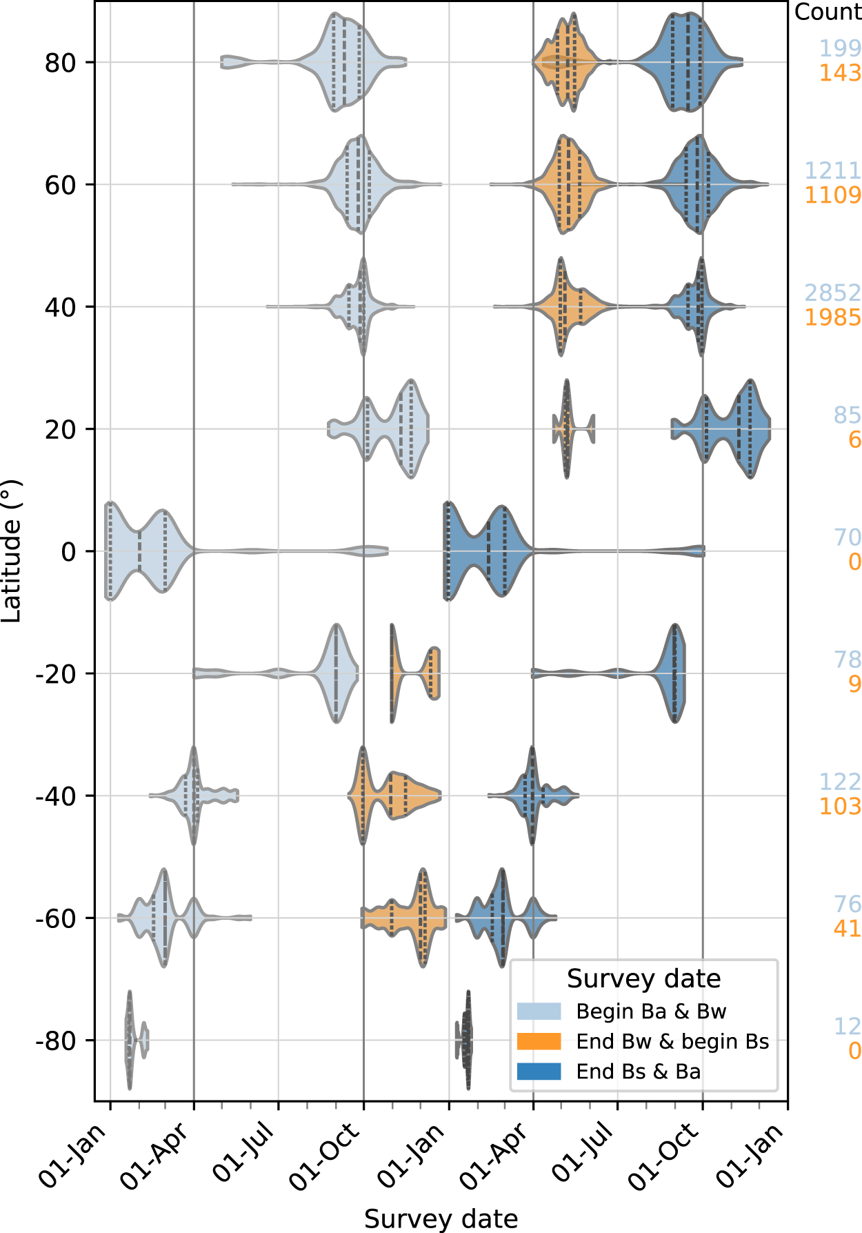
Glaciological measurements are typically designed to measure the mass balance over hydrological years, often starting 1 October (1 April) in the Northern (Southern) Hemisphere. However, the exact timing and duration of reported annual and seasonal balances vary significantly, as illustrated in Fig. 4, which displays the glaciological survey dates of annual and seasonal balances reported to the World Glacier Monitoring Service (WGMS) (WGMS, 2024). In the Northern Hemisphere, glaciological surveys are typically carried out between mid-August and mid-October. In the mid-latitudes of the Southern Hemisphere, they typically occur in April and May, whereas on the few glaciers observed in the (sub-)Antarctic islands, they occur in January or February (Fig. 4).
Violin plot showing the density distribution of glaciological survey dates aggregated by 20° latitude bands. Distributions are shown for the start and end dates of annual balances (B a), and mid-season dates that separate the end of the winter (B w) and the beginning of the summer balance (B s) periods. Vertical dashed and dotted lines refer to median and first and third quantiles, respectively. The count of survey dates per latitude bin for annual (blue) and winter/summer (orange) balances is given on the right. Source: WGMS (2024).

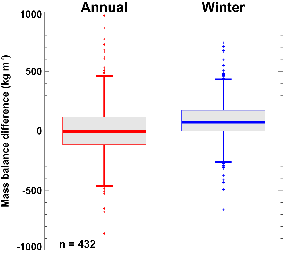
Observed (or modeled) annual balances can vary significantly depending on the time system, as the corresponding duration, along with the start and end dates of the mass-balance year, differs between these systems. In the fixed-date system (Cogley and others, Reference Cogley2011), dates are constant and each mass-balance year is exactly 12 months long. However, this is not the case in the floating date time system (defined by varying survey dates) and the stratigraphic system (defined by dates of sequential annual mass minima/maxima). To quantify discrepancies in annual and seasonal mass balances between the most commonly reported fixed- and floating date time systems, we compared the corresponding glacier-wide mass balances for 11 Swiss glaciers. Balances were derived from a daily-resolution distributed mass-balance model constrained by seasonal point observations (Huss and others, Reference Huss, Dhulst and Bauder2015; GLAMOS, 2024). This allows extracting mass balance over arbitrary time periods. Results indicate that absolute median differences between annual/winter balances derived from actual measurement dates and those based on a fixed-date system were less than 100 kg m−2 (0.1 m w.e.); however, individual cases can be an order of magnitude greater (Fig. 5).
Boxplot of difference of glacier-wide annual and winter mass balance between a fixed-date period (annual: 1 October–30 September, winter: 1 October–30 April) and the actual measurement period (floating-date system) for 11 Swiss glaciers with long-term monitoring starting between 1914 and 2012 and extending until 2024 (n = 432). Since the start date is unknown, for the winter balance, the start of the measurement period is the day of the modeled (glacier-wide) mass minimum (i.e. stratigraphic date). Whiskers extend to the furthest data points that lie within 1.5 times the interquartile range from the quartiles. Crosses refer to outliers. Absolute deviations of measurement dates from 1 October and from 30 April were 12 ± 12 days and 0 ± 22 days (mean ± standard deviation), respectively.

Accounting for deviations of the time span from full mass-balance years can be further complicated by the fact that the exact time spans of mass-balance estimates are often ill-defined or simply unknown. For example, for glaciological balances derived in the stratigraphic system, the dates of mass minima are typically not known. In addition, many glaciological mass balances reported to the WGMS lack information on the time system and/or dates and duration of each balance’s time span. Out of 8298 mass-balance records on 516 glaciers, only 4705 records (57%) on 296 glaciers include the start and end dates with the reported annual balance. Mid-season dates, referring to end-of-winter and beginning-of-summer balances, are reported for 3396 records on 222 glaciers (WGMS, 2024; Fig. 4).
3.3.2. Geodetic balances (surface elevation differencing)
DEM differencing relies on the availability of DEMs, which typically are not designed or acquired specifically for glaciological purposes. As a result, these balances may refer to any date in the year, and corrections are needed to make the balances comparable to balances that refer to one or multiples of full mass-balance years. The magnitude of these corrections depends on the mass changes that occur over the deviating period. For example, Yang and others (Reference Yang, Hock, Kang, Shangguan and Guo2020) found that the mass-change rate of all glaciers of the Kenai Peninsula in Alaska (>4000 km2) averaged over 9 years would have been underestimated by 0.09 m w.e. a−1 (∼10%) if the difference in acquisition dates of the earlier ASTER and the later IFSAR DEM had not been corrected for, despite the dates being only 27 days apart. Differences between uncorrected and seasonally corrected balance rates for an ice cap in Iceland reached up to 0.4 m w.e. a−1 when spanning shorter periods (4–6 years), but they were negligible for periods exceeding 20 years (Belart and others, Reference Belart2020). The largest required annual correction was almost 2 m w.e. for a DEM acquired two months before the end of the mass-balance year. For another Icelandic ice cap, one of the DEMs had to be corrected by an average elevation of 3.5 m, which corresponded to roughly three-fourths of the entire thickness change during the considered 15-year period. These examples underscore the critical importance of (i) accounting for differences in DEM acquisition dates especially in regions with large mass turnover and (ii) targeting DEM acquisitions, as much as possible, at a similar time of the year (Berthier and others, Reference Berthier2023).
In addition, DEMs or maps are often composed from sources referring to different dates, sometimes years apart, in different parts of the glacier or glacier region (e.g. Braun and others, Reference Braun2019), but mass balances are reported for one single (average) period. Instead of traditional DEM differencing from just two surveys, geodetic balances are increasingly derived from multi-survey regressions at pixel scale (see Section 2.2.1), further complicating precise determination of the time span especially when applied over larger regions. For example, Dussaillant and others (Reference Dussaillant2019) used 30 000 ASTER DEMs to determine the mass change over the entire Andes between 2000 and 2018. Although the first DEM was acquired in March 2000 and the last DEM in April 2018, in reality, the start and end dates varied substantially over the domain due to data availability and clouds. Averaged for their seven sub-regions, the mean start date ranged from June 2000 (Fuegian Andes) to December 2001 (North Patagonia). The mean end dates varied from March 2016 (Fuegian Andes) to November 2017 (Central Andes), thus covering differences in period lengths exceeding the length of an entire summer or winter season.
Similar challenges may also occur with other sources of elevation data. For example, the ICESat laser altimetry satellite acquired data between 2003 and 2009 in distinct campaigns in February/March and October/November each year, as well as May/June in some years. This non-continuous temporal sampling requires particular vigilance to avoid seasonal variations introducing bias into the trends. Bolch and others (Reference Bolch2013) used ICESat data from October 2003 (end of the ablation period) to March 2008 (end of the accumulation period) to determine mass changes in Greenland’s peripheral glaciers. They estimate a mass loss of 27.9 ± 10.7 Gt a−1. Also using ICESat, Gardner and others (Reference Gardner2013) estimated a loss of 37.7 ± 6.6 Gt a−1 between October 2003 and October 2009. The lower losses reported by Bolch and others (Reference Bolch2013) may result from not accounting for seasonality, though differences in densification corrections could also play a role.
3.3.3. Gravimetric method (GRACE)
The GRACE satellites provided their first data in April 2002, and it is common practice in the GRACE community to report mass balances from this date up to the most recent observations. Hence, reported average rates often do not coincide with a full mass-balance year or refer to an integer number of years. For example, Ciracì and others (Reference Ciracì, Velicogna and Swenson2020) reported average mass-balance rates for the period April 2002–September 2019. Wouters and others (Reference Wouters, Gardner and Moholdt2019) reported rates for April 2002–August 2016, albeit they also included estimates for periods with complete mass-balance years (October 2005–September 2015 in the Northern Hemisphere and April 2005–March 2015 in the Southern Hemisphere).
3.3.4. Simulating the impact of deviations from full mass-balance year
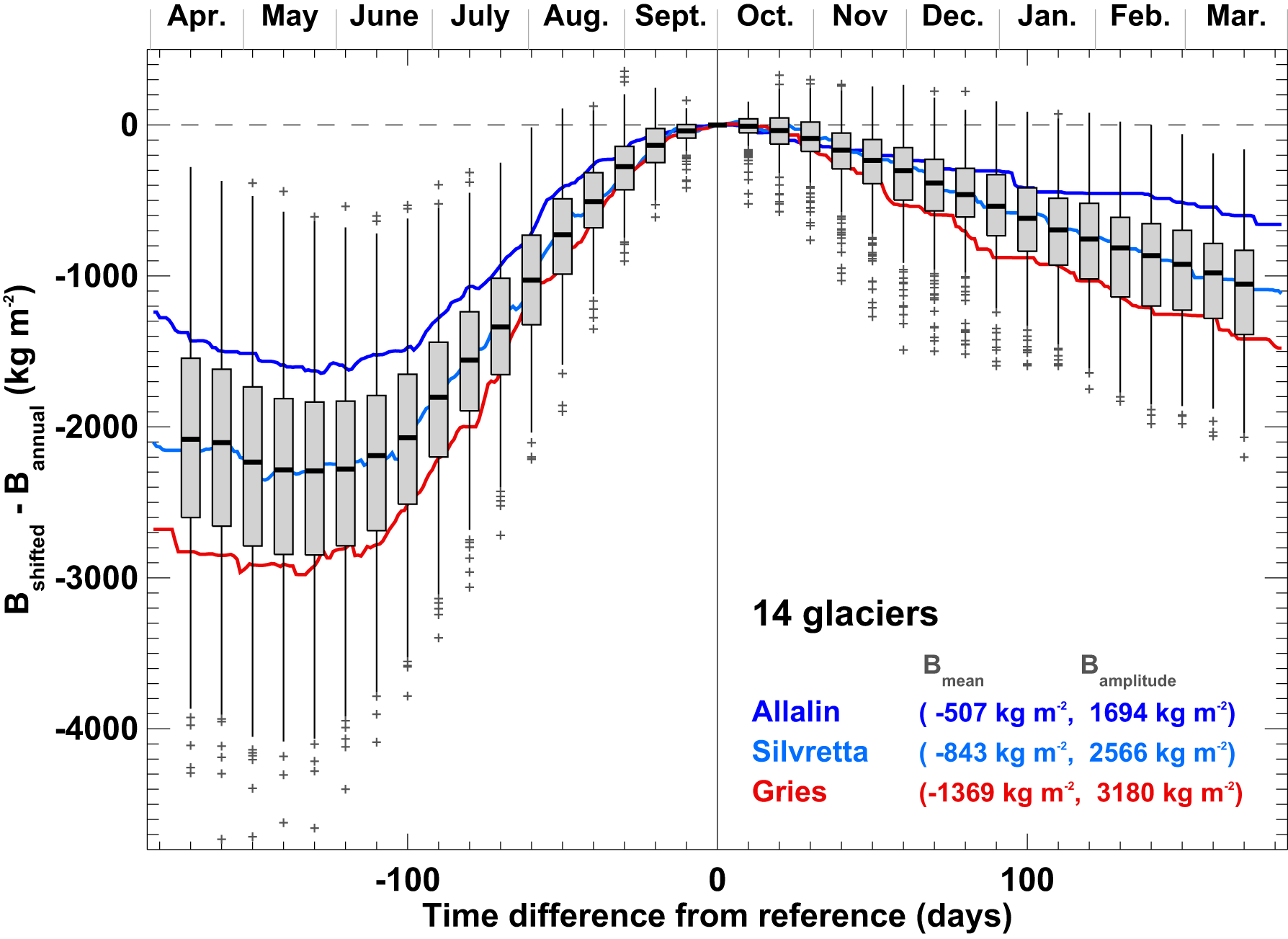
Mass balances are often reported as annual balances. However, regardless of the method of determination, mass balances are expected to increasingly diverge from the true annual balances as the duration deviates from a full year. To illustrate the effect of survey dates on mass balance, we simulated the glacier-wide daily mass balances of 14 glaciers in the Swiss Alps for the mass-balance years 1999/2000 through 2019/2020 constrained with seasonal in situ observations. We then recalculated each year’s mass balance by shifting the start date of the balance year by up to 170 days in both directions from a reference date of 1 October and computed the difference to each annual balance ending on 30 September of the following year. The results indicate that differences are generally small for shifts of up to 20 days but increase rapidly as the deviation from the reference date grows (Fig. 6). Outliers show that in certain years, even small shifts in the start date can result in substantial differences. However, when calculating multi-year averages, absolute differences will steadily decrease with each additional year. As expected, the results for Allalin, Silvretta and Gries Glacier confirm that the differences increase as the annual mass-balance amplitudes as well as discrepancies from balanced conditions grow. The effect of shifts in the observation date, for example, caused by image acquisition schedules, will thus be smallest for glaciers in more continental climates with low mass-loss rates and highest for maritime glaciers with rapid mass-loss rates.
Box plot of differences in mass balance over a full year (B annual; 1 October to the following 30 September) and the balance over longer/shorter periods (B shifted) as a function of deviation of mass-balance year-end data from the reference date. Data are based on 14 Swiss glaciers in the period 2000–2020 and derived from a mass-balance model constrained by in situ observations (Huss and others, Reference Huss2021). Results are aggregated in 10-day periods. The difference is also shown for three glaciers, each color-coded to represent different seasonal mass-balance amplitudes: low (Allalin), intermediate (Silvretta) and high (Gries). Whiskers extend from the box to the furthest data points that lie within 1.5 times the interquartile range from the quartiles. Crosses refer to outliers.

Figure 6 also demonstrates that the differences are asymmetric around the reference date, with notably greater discrepancies occurring when end dates are shifted earlier, i.e. into the summer season, than later toward winter. This can be attributed to the overall negative annual balances during this period, where summer mass losses surpass winter mass gains. Consequently, when planning satellite stereo acquisitions, deviations from the end of the mass-balance year toward winter are less problematic than deviations toward summer.
3.3.5. Compounding impact of seasonal snow
When deriving mass change from surface elevation differencing with a constant conversion factor, the impact of survey dates that do not align with full-year mass-balance years can be significantly amplified if the glacier is partially or fully covered by snow on one of the survey dates. Since seasonal snow typically has a density of less than half that of the widely used conversion factor of 850 kg m−3, the mass balance can be significantly overestimated or underestimated if the generally lower density of seasonal snow is not considered in the conversion to mass change. The difference is expected to increase with the amount of seasonal snow depth and thus will be greatest when the survey period begins in spring but ends in fall or vice versa.
3.4. Spatial domain and area
Accurate identification of the spatial domain and glacier area is critical but complicated by glacier area changes in response to mass change as well as methodological and data constraints. For example, regional GRACE mass-balance estimates can be contaminated by leakage from mass changes in adjacent regions. In the glaciological method, point balances are extrapolated across the current glacier area; however, in practice, maps are often not updated for years, thus invoking biases in the annual estimates (Zemp and others, Reference Zemp2013).
Regardless of the method used, the precise knowledge of glacier area at the survey dates is particularly important when balances are converted to or from specific units, i.e. the mass change divided by unit glacier area. The issue becomes increasingly important as the relative area change increases. Multi-year balances from surface elevation surveys face the problem of which area to use when the glacier area has changed between survey dates. In such cases, often the glacier areas of two consecutive surveys coinciding with or close to the start and end dates of the mass-change period are simply averaged (e.g. Fischer and others, Reference Fischer, Huss and Hoelzle2015; Seehaus and others, Reference Seehaus, Malz, Sommer, Lippl, Cochachin and Braun2019), but sometimes only the earlier area or latter area or any other mapped area closest to the mass-change period is used when no repeat information is available (e.g. Braun and others, Reference Braun2019). Some studies linearly interpolated between mapped areas when deriving specific mass-balance time series (Hugonnet and others, Reference Hugonnet2021). For five glaciers in North America, assuming a fixed maximum area rather than incorporating temporal retreat underestimated DEM-differencing-derived mass loss by 19%, highlighting the need to incorporate temporally resolved area changes (Florentine and others, Reference Florentine, Sass, McNeil, Baker and O’Neel2023).
4. Discussion and recommendations
The issues outlined above can hinder the comparability of published mass-balance estimates, particularly when they were derived from different methodologies. These challenges also complicate the process of synthesizing estimates from individual regions across various studies into global estimates. To address these concerns and ensure clarity, comparability and utility of glaciological data across studies, we propose the following recommendations that build upon and expand previous suggestions in the literature (e.g. Cogley and others, Reference Cogley2011; Berthier and others, Reference Berthier2023; Piermattei and others, Reference Piermattei2024; WGMS, 2024). Our recommendations hold equally for glacier and ice-sheet mass-balance reporting. They also generally hold for balances generated by numerical mass-balance models driven by climate data.
4.1. Definition of time span
Authors should explicitly define the time span of each reported mass balance by stating the precise start and end dates. This is important irrespective of the observational method or the duration of the mass-balance period, whether it is seasonal, annual, multi-year or any other time period. For glaciological balances, the time system used — whether fixed-date, floating-date, stratigraphic or combined — should be indicated, along with any applied corrections to align measurements with those definitions. In case of stratigraphic observations, it is useful to report an estimated reference date with plausible uncertainty. Such information is also necessary for geodetic balances when seasonal bias corrections are implemented to align with the targeted time period (typically a full year or its multiples). Annual balances and multi-year averages should be adjusted to and reported over periods of complete years to minimize seasonal bias. While less straightforward for balances derived from the glaciological method or DEM differencing, regional or global-scale modeled balances should also be reported over calendar years to improve compatibility with sea-level assessments.
Precise definition of the time span is particularly important for comparing observations with estimates from mass-balance models (Huss and Hock, Reference Huss and Hock2015). If a model is run with a sufficiently short time step, modeled mass change can be extracted over any period of time to match the exact period of the observation (Barandun and others, Reference Barandun2018). However, this is only possible if precise start and end dates are reported for each observational balance, whether it pertains to point, glacier-wide or region-wide mass balance.
4.2. Definition of domain
It is crucial to clearly define the spatial domain, specifying whether it covers an entire glacier, subregions thereof, or a collection of glaciers in a region. If balances are expressed in specific units, the glacier area used for the calculation should be given. If time-evolving areas are used, e.g. for annual balances, the area values at each time step should be reported. While mass balances reported in specific units can in principle be reported for any part of a glacier, only those covering one or more entire glaciers yield meaningful comparisons with other glaciers or regions, given the typical pronounced elevation-dependence of mass balance.
To support multi-study intercomparison and synthesis, regional-scale estimates should ideally be calculated and reported for glacier regions defined by the Global Terrestrial Network for Glaciers (GTN-G, 2023), which coincides with the regions of the Randolph Glacier Inventory (RGI; RGI Consortium, 2023). For estimates using existing glacier inventories, one should identify the inventory and version (e.g. RGI version 6 or 7), including any exclusions, for example, below a minimum glacier size. If the used glacier inventory data are not already in the public domain, then they should be included alongside the reported mass balance. Glacier outlines should be submitted to the GLIMS glacier database hosted at the US National Snow and Ice Data Center (NSIDC; Raup and others, Reference Raup, Racoviteanu, Khalsa, Helm, Armstrong and Arnaud2007), which also serves as the exclusive source for RGI version 7 and onward.
Gravimetry-derived balances may be affected by signal leakage from adjacent regions. Thus, authors should describe how domains were handled to minimize ambiguity.
4.3. Mass-balance components and terminology
Not all methods yield total mass change (Section 3.2), so it is crucial to specify which components are included and which may be omitted. For example, does a reported mass balance capture mass change below the ocean or lake level? Does it include frontal ablation, basal melt or refreezing?
In this context, proper terminology is crucial. For example, the term surface mass balance has been used ambiguously in the literature. While strictly speaking defined as the balance between accumulation and ablation at the surface (typically measured by the glaciological method), the term has been extended, in particular by the ice-sheet community, to also include refreezing in the ice sheets’ thick firn layers (e.g. Rignot and others, Reference Rignot, Box, Burgess and Hanna2008; Rahlves and others, Reference Rahlves, Goelzer, Born and Langebroek2025). Given that refreezing can be a major component of the mass budget (e.g. ∼50% of all melt refreezes within the Greenland ice sheet; van Dalum and others, Reference van Dalum2024), the distinction is far from merely academic, in particular for ice sheets. To address this ambiguity, Cogley and others (Reference Cogley2011) introduced the term climatic mass balance to refer to the sum of surface and internal mass balance, and the term climatic-basal mass balance if basal mass changes are included as well, to distinguish it unambiguously from the term surface mass balance. Overall, to improve clarity and comparability of reported mass balances of glaciers and ice sheets, we recommend adhering to the mass-balance terminology established by Cogley and others (Reference Cogley2011).
We also note that the term ‘geodetic method’, historically used in glaciology to describe surface elevation differencing (Cogley and others, Reference Cogley2011), has become ambiguous due to the growing prominence of the gravimetric method since the launch of the GRACE satellite in 2002. Therefore, we caution against its use in the former context whenever possible, or at least ensure that a clear definition is provided. When comparing methods, it is thus crucial to specify whether mass balances were derived from the gravimetric method (e.g. GRACE) or from surface elevation differencing (using DEMs or observations along flight/satellite tracks).
4.4. Units
All reported values should include sufficient information to enable conversion between units (e.g. from Gt to kg m−2 or SLE). Depending on the method, this includes the values of glacier area used to convert mass units to specific units and vice versa, as well as the conversion factor(s) used to convert between volume and mass. SLE estimates should provide the ocean area used in the calculations, detail the conversion process and specify the water densities if ice that displaced ocean water was accounted for.
We recommend using kg m−2 as the preferred unit for specific mass balance instead of the traditional and widely used unit m w.e., as it clearly conveys mass without any ambiguity regarding ice or snow density. Glacier-wide and regional estimates should ideally be presented in both mass and specific units, and global estimates should include SLEs to facilitate comparability across studies. When feasible, mass balances should also be reported as annual balances, in addition to multi-year averages.
4.5. Uncertainties
Mass-balance estimates (point, glacier-wide and regional/global) should be accompanied by statements of uncertainty; however, reported glaciological mass balances of individual glaciers usually lack them (WGMS, 2024). Regional-scale estimates generally include uncertainties; however, methods vary greatly among studies complicating direct comparison. Thus, developing community-based procedures for each principal method would be beneficial. At a minimum, uncertainty estimates, regardless of method, should include the associated probability range (e.g. one-sigma or two-sigma), assumptions made (e.g. how errors are propagated, correlation length scales) and sufficient details on their derivation to ensure reproducibility. When formal derivation of errors is not possible, it is recommended that the author provide an ‘expert judgment’ of the uncertainties accompanied by a justification, preferably with citations to existing peer-reviewed literature. When possible, spatially resolved estimates of glacier mass change should be accompanied by a spatially explicit error field.
4.6. Calculation methods, raw data and reproducibility
When reporting mass balance, it is essential to describe in detail the processing steps used to derive the balance. We note that mass balances from all three observational methods involve various assumptions or modeling steps. Thus, the distinction between observed, reconstructed and modeled mass balances is somewhat blurred (Geibel and others, Reference Geibel, Huss, Kurzböck, Hodel, Bauder and Farinotti2022). For instance, glacier-wide balances obtained through the glaciological method typically rely on statistical models for spatial extrapolation of the point balances, while methods based on elevation differencing require assumptions or models to determine the conversion factor from volume to mass, and gravimetrically derived estimates rely on models to account for mass changes from processes other than glacier mass change. Thus, transparency in data sources, analytical approaches, interpolation techniques (spatial and temporal) and parameter choices is essential for reproducibility and reinterpretation. For example, despite prescribed source data, a comprehensive inter-comparison project of geodetic balances revealed large disparities in derived glacier-wide surface elevation change rates (Piermattei and others, Reference Piermattei2024), underscoring the need to detail individual processing steps to identify their sources.
For estimates based on surface elevation differencing, this includes being explicit about the volume-to-mass conversion factors or firn models applied. Additionally, one should describe void-filling techniques and include void-filled elevation change fields, masks for voids or interpolated areas, off-ice elevation change fields and layers indicating data coverage, the number of data per pixel over time as well as start and end dates. When derived from sources with disparate surface elevation survey dates across the investigated domain, an additional layer that specifies for each pixel the start and end survey dates should be provided.
For glaciologically derived estimates, it is essential to clarify the density assumptions used to convert stake readings and snow depths to mass, and the spatial interpolation techniques used to extrapolate point observations. We further recommend that glacier-wide balances be consistently accompanied by the reporting of the individual point balances, including their precise spatial coordinates, elevation and sampling dates. Point balances are invaluable for model calibration and evaluation (Huss and Hock, Reference Huss and Hock2015), as they avoid the substantial uncertainties associated with spatial extrapolation (Hock and Jensen, Reference Hock and Jensen1999). Ideally, the raw data underlying the derived point balances (such as the original stake readings) are also made available.
For gravimetry-based estimates, authors should include information on the corrections applied (e.g. glacial isostatic adjustment, including possible Little Ice Age effects, terrestrial water storage, dynamic oblateness correction, Earth center of mass correction), what non-glacier signals have not been corrected for (i.e. terrestrial snow, reservoir change) and how the temporal gap between GRACE and GRACE Follow-On (from July 2017 to May 2018) has been handled. All gravimetry-derived estimates should publish raw time series, spatial domain of integration and corrections.
Regardless of the method, including the underlying data and metadata, for example as supplementary information, empowers future studies to apply alternative processing steps, updated models or assumptions. Thus, future users can reprocess results to suit evolving methodologies or science goals.
4.7. Open data
Glacier mass-balance data and their underlying raw data should be made publicly available to promote transparency and accessibility in accordance with the FAIR principles (Findable, Accessible, Interoperable and Reusable) (Wilkinson and others, Reference Wilkinson2016). Where appropriate, this should also be extended to the source code used to derive a reported mass balance from the raw data.
Glaciological glacier-wide balances have traditionally been archived by the WGMS in Zürich, Switzerland. In recent years, this archive has also expanded to include point balances and glacier-wide balances based on elevation differencing. The NSIDC in Boulder, USA, hosts a diversity of glacier inventories (GLIMS and different versions of the RGI), glacier mass-balance observations and model results with an emphasis on remote-sensing observations.
In addition, many mass-balance data are archived in open-access repositories such as the information system PANGAEA or Zenodo. However, centralized archives, as opposed to disparate data stores located in various places, are preferable as they facilitate uniform access and promote data standardization. Alternative solutions are still necessary to enable more comprehensive reporting of the underlying raw data and intermediate data products that centralized data centers typically do not support, such as distributed elevation change grids or ablation stake readings. Currently, gravimetry-derived observations are not archived in a centralized repository. We thus recommend that these observations are also curated by one of the international data centers to enhance accessibility and usability.
In recent years, we have experienced an exponential growth in glacier observations from remote sensing. The compilation, management and dissemination of this wealth of data become an increasing challenge for the notoriously underfunded international data centers (WGMS, NSIDC) and their databases (e.g. GLIMS, RGI). An increase in their long-term support is fundamental for the scientific community to continue and improve regional- to global-scale assessments.
5. Conclusions
Significant challenges emerge when comparing or synthesizing glacier mass-balance estimates from different sources and methods into regional and global estimates. These difficulties arise from lack of crucial information, inconsistent reporting and limitations inherent to the commonly employed glaciological, geodetic or gravimetric methods. Thus, there is an urgent need for more rigorous and standardized reporting of glacier mass-balance observations of both glaciers and ice sheets. For example, estimates must clearly specify the domain, the time period and included mass-balance components, along with sufficient information for converting to other commonly used mass-balance units to facilitate comparisons among studies. In addition, it is crucial to detail all processing steps used to derive a mass balance, including relevant equations, assumptions, parameter values and corrections. Ideally, underlying raw data and other relevant datasets used in the calculations are also made available to allow full reproducibility and reinterpretation, enhance scientific utility and promote transparency. Authors, reviewers, editors and data centers all share a collective responsibility to ensure the implementation of these improved reporting practices.
Data availability statement
The data and code for Figures 1, 2, 5 and 6 are available at https://zenodo.org/records/18959574.
Acknowledgements
This paper evolved from the Working Group on the Regional Assessments of Glacier Mass Change (RAGMAC) supported by the International Association of Cryospheric Sciences (IACS). R.H. was supported by the Norwegian Research Council (grant 324131 GLACMOD), the ERC-2022-ADG 101096057 GLACMASS and NASA grants 80NSSC20K1296 and 80NSSC20K1595. M.H.B. was supported by DFG grants (BR2105/14-1+2, BR2105/28-1 ITERATE and BR2105/29-1 CSAPIS) as well as through the International Doctorate Program M3OCCA funded by the Bavarian State Ministry of Science and The Arts through its Elite Network Bavaria. A.G.’s contributions were carried out at the Jet Propulsion Laboratory, California Institute of Technology, under a contract with the National Aeronautics and Space Administration (80NM0018D0004). E.B. acknowledges support from the French Space Agency (CNES) and M.Z. from the Federal Office of Meteorology and Climatology MeteoSwiss within the framework of GCOS Switzerland. We thank Martin Truffer for valuable input to Figure 3, scientific editor David Rounce for handling this manuscript and Shashank Bhushan and an anonymous reviewer for their reviews.
Author contributions
RH initiated and designed the study, and wrote the paper with significant edits from all co-authors. AG and BW contributed text to the Recommendations and GRACE sections, respectively. MH made three figures, and performed the related calculations; BW, MZ, EB and MHB made the remaining three figures, with input on content and design from RH. All authors, in particular MH, discussed the content, and commented on the manuscript.

 Open access