Introduction

The problem of understanding the response of Himalayan glaciers to climate change has attracted much attention (Reference RainaRaina, 2009; Reference CogleyCogley, 2011; Reference Scherler, Bookhagen and StreckerScherler and others, 2011a; Reference BennBenn and others, 2012; Reference BolchBolch and others, 2012; Reference Jacob, Wahr, Pfeffer and SwensonJacob and others, 2012). The variable response of Himalayan glaciers has prevented a coherent interpretation of the data (Reference Scherler, Bookhagen and StreckerScherler and others, 2011a; Reference BolchBolch and others, 2012). For instance, according to the remote-sensing study by Reference Scherler, Bookhagen and StreckerScherler and others (2011a), in the south central Himalaya, while most (65%) of the glaciers are retreating, a significant fraction (35%) are almost stationary or advancing. Reference Scherler, Bookhagen and StreckerScherler and others (2011a) highlighted the importance of the role of supraglacial debris cover in the dynamics of the response of these glaciers to changes in the climate. One peculiar feature they observe is the existence of many stagnant glaciers. These have stationary fronts and very low ice velocities (<2.5 m a⁻¹) in the tongue regions. All such glaciers have a large (>40%) extent of debris cover. Their data also reveal a difference between the front velocities (retreat/advance rates) of debris-covered and debris-free (bare) glaciers. To illustrate this we separate their sample into sparsely (<10% extent) debris-covered glaciers and extensively (>10% extent) debris-covered glaciers. Of the 255 glaciers for which they measured frontal retreat rates, 66 are in Hindu Kush, Karakoram and the west Kunlun Shan and 189 in the Himalaya. In this work we consider only those that are in the Himalaya. Of these 189 glaciers, 128 have extensive debris cover and 61 have sparse debris cover. We further classify these glaciers as retreating (front velocity <−5 m a⁻¹), stationary (−5 m a⁻¹ < front velocity < 5 m a⁻¹) and the rest as advancing. Of the 61 sparse-debris glaciers, 82% are retreating and 18% are stationary/ advancing, whereas of the 128 extensive-debris glaciers, 52% are retreating and 48% are stationary/advancing. These differences are puzzling, as the two types of glaciers are not regionally separated and must be experiencing similar climates.

In this paper we address three puzzles posed by the work of Reference Scherler, Bookhagen and StreckerScherler and others (2011a). Why are there such a large number of ‘stagnant’ glaciers? Why is there a discrepancy between the average behaviours of extensively debris-covered glaciers and sparsely debris-covered ones? Why is there such a large variation in the frontal retreat rates of glaciers in the Himalaya?

To answer the first two questions, we formulate and study a simplified flowline model of debris-covered glaciers. We validate this model against data on Dokriani Glacier (Reference Dobhal, Gergan, Thayyen and MahéDobhal and others, 2007). The analysis reveals that glaciers with extensive debris cover have a qualitative difference in their response to a warming climate as compared with bare glaciers. A debris-covered glacier has larger climate sensitivity than a bare glacier with the same equilibrium-line altitude (ELA). The dynamical response of an extensively debris-covered glacier to a warming climate is characterized by two timescales. For an initial period, which can be over a century, the front of the glacier is almost stationary and it develops a slow-flowing tongue. During this period, the glacier steadily loses ice volume by thinning. After this initial period it retreats with a rate characterized by a second timescale. Thus we conclude that the observed stagnant glaciers (Reference Scherler, Bookhagen and StreckerScherler and others, 2011a) are losing ice volume. We therefore reclassify the retreating and stagnant glaciers together and refer to them as shrinking glaciers. The fraction of shrinking glaciers in the sample with extensive debris cover (73%) then becomes about the same as the corresponding fraction in the sample of sparsely debris-covered glaciers (82%).

We then attempt to understand the large variation in the front retreat rates. The retreat rate of a glacier depends on the local climate and its geometrical properties (slope, length, etc.). Both the local climate and the geometry vary from glacier to glacier. A simple and natural framework to quantitatively describe these effects is Reference OerlemansOerlemans' (2005) model. The model describes the length changes of a glacier in response to changes in the local temperature, and was effectively used by Oerlemans to reconstruct the global average temperature history for the past four centuries. However, our results show that the complex lag effects (involving two timescales) of the response of extensively debris-covered glaciers to temperature change are not described by Reference OerlemansOerlemans' (2005) model as it stands. In the absence of a generalized model to describe the response of extensively debris-covered glaciers, we concentrate on the set of 61 sparsely debris-covered glaciers in the Himalayan region. We use Oerlemans' model, in the context of a particular climate scenario, to extract the warming rate experienced by each glacier. We thus obtain the distribution of warming rates corresponding to the observed glacier retreat rates. We compare this with the distribution of warming rates obtained from the available weather station data in the region. The two distributions have similar average values and standard deviations. While this agreement does not imply that the weather station data are correlated with the glacier data, it does suggest that the observed variation in the front retreat rates is compatible with the observed variation in the glacier geometries and local climate.

Debris-Covered Glaciers

Here we review past work on debris-covered glaciers, which motivates the model that we study in detail.

The debris layer and the ice are strongly coupled. The debris is transported by the ice and the ice flow is influenced by the debris. The debris exerts a small extra driving force on the ice surface and strongly affects the local ablation. The former effect is not very important, as the ice equivalent of the debris thickness is small compared with the ice thickness. However, experimental and theoretical work (Reference Nakawo and YoungNakawo and Young, 1981, Reference Nakawo and TakahashiNakawo and Takahashi, 1982; Reference Mattson, Gardner and YoungMattson and others, 1993; Reference Conway and RasmussenConway and Rasmussen, 2000; Reference KonovalovKonovalov, 2000; Reference Nicholson and BennNicholson and Benn, 2006; Reference BennBenn and others, 2012) shows that the ablation properties are significantly affected. The debris layer reduces the albedo and provides thermal insulation to the ice. Up to a thickness of ∼1 cm (Reference Mattson, Gardner and YoungMattson and others, 1993), the former effect is dominant and results in an increased rate of ablation. At larger thicknesses, the latter effect dominates, resulting in a significant decrease in the ablation rate.

The debris deposited in the accumulation zone subsides into the ice and emerges in the ablation zone with the melting ice. Thus the debris accumulates on the glacier surface as ice flows down the valley, thickening the debris layer there. The ice velocity in the ablation zone decreases in the downstream direction, causing the debris to pile up. Typically, there are also rockfalls on the valley sides, feeding debris into the glacier. Hence the debris thickness increases in the downstream direction and decreases the ablation rates. This decreasing trend can counteract or overcome the increasing trend due to the increase in temperature at lower elevations. Consequently, the specific mass-balance functions of glaciers with thick debris layers may decrease to a minimum or have a kink (a rapid change in slope) at some altitude, E _K, in the ablation zone. Below E _K it either becomes more-or-less independent of the altitude or increases in the downstream direction, as illustrated in Figure 1b and c.

Fig. 1.

Mass-balance profiles for debris-covered glaciers. (a) Mass-balance profile of the bare glacier Nigardsbreen, Norway (Reference Haeberli, Zemp, Kääb, Paul and HoelzleWGMS, 2008). (b) Mass-balance profile of the debris-covered Chota Shigri Glacier, Indian Himalaya (Reference WagnonWagnon and others, 2007). (c) Three examples of the idealized mass-balance profiles used in this paper. Note that above elevation E _K the profiles coincide and the value of the balance gradient is β. Also note that for debris-covered glaciers the mass-balance curve has a kink at E _K. For these glaciers the balance gradient below E _K takes the value (β – β′)

Some models of this coupled dynamics have been reported in the literature. These are flowline models with two variable functions, the debris-thickness profile and the ice-thickness profile. There is a set of two coupled equations which describes the dynamics. Reference Konrad and HumphreyKonrad and Humphrey (2000) studied the steady-state properties of rock glaciers, Reference Naito, Nakawo, Kadota and RaymondNaito and others (2000) modelled Khumbu Glacier and Reference Vacco, Alley and PollardVacco and others (2010) investigated the effects of a debris avalanche on the ice dynamics, using such models.

In the next section, we use a simpler model of a debris-covered glacier, that captures the essential physics of the effect of the debris layer.

A Flowline Model for Debris-Covered Glaciers

As discussed above, there is a qualitative difference in the specific mass-balance profiles of debris-covered and bare glaciers. The profile smoothly decreases in the downstream direction for bare glaciers, whereas for debris-covered ones there is a sharp change in slope somewhere in the ablation zone. In several cases the slope changes sign, leading to a minimum located in the ablation zone. We have studied the effects of the existence of this kink in the specific mass-balance profile in an idealized glacier model, the flowline model (Reference OerlemansOerlemans, 2001; Reference Adhikari and HuybrechtsAdhikari and Huybrechts, 2009). The glacier is modelled as ice flowing in a channel described by the cross-section-averaged ice thickness, H(x, t), and velocity, u(x, t), profiles; t is the time and x the coordinate along the central flowline. The ice-volume equation is

(1)

where W(x) is the cross-sectional area and b(x, t) the specific mass-balance profile. Given the form of the mass-balance profile, b(x, t), together with a constitutive relation between the velocity and the ice thickness, Eqn (1) can be solved for the thickness and velocity profiles. We take the constitutive relation to be (Reference OerlemansOerlemans, 2001)

(2)

where ρ is the ice density, g the acceleration due to gravity and z(x) the bedrock profile, which we take to be linear with slope, s; f _d is the constant associated with the deformation flow (Glen’s law) and f _s parameterizes the basal slip.

We have used a piecewise linear mass-balance profile, b(x), that incorporates effects of the debris layer in a minimal way,

(3)

where h(x, t) ≡ H(x, t) + z(x) is the ice surface altitude, with H(x, t) the ice thickness and β′ ≥ β > 0. This idealized profile, parameterized by the ELA, E, the altitude of the kink, E _K, and the two gradients, β and β′, is plotted in Figure 1 c for some sample parameters. The value of E − E _K can be expected to decrease with increasing debris source strengths and ice velocity gradients. Its value in the measured mass-balance profiles of some debris-covered Himalayan glaciers (e.g. Khumbu (Reference Benn and LehmkuhlBenn and Lehmkuhl, 2000), Chota Shigri (Reference WagnonWagnon and others, 2007) and Dokriani (Reference Dobhal, Gergan, Thayyen and MahéDobhal and others, 2007)) lie in the range 400–700 m.

Changes in the climate influence the glacier dynamics through changes in the mass-balance profile which, in turn, depends on both the climate and the ice/debris dynamics. We make the simplifying assumption that for small changes in temperature the ELA responds instantly to the changes and the balance gradients, β and β′, remain unchanged. We have investigated two extreme possibilities for the change in E _K: (1) the limit of fast debris response where E _K changes instantly, keeping E − E _K fixed, and (2) the limit where E _K remains fixed.

In the next section, we use this assumption in a flowline model of a real glacier to check its validity.

Validation of the Model

We have validated this model against data for Dokriani Glacier. Dokriani is a well-studied glacier (Reference Gergan, Dobhal and KaushikGergan and others, 1999; Reference Hasnain and ThayyenHasnain and Thayyen, 1999; Reference Dobhal, Gergan, Thayyen and MahéDobhal and others, 2007) located in the Bhagirathi Basin, Garhwal Himalaya (30’51°N, 78’49°E). It is ∼5.5 km long and has an area of ∼6 km². About 40% of the glacier area is covered with supraglacial debris (Reference Hasnain and ThayyenHasnain and Thayyen, 1999). Below we describe a simplified approximate numerical model of Dokriani Glacier.

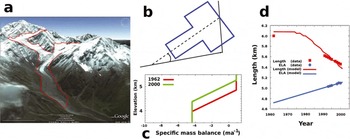
We approximate this glacier with a rectangular channel with a uniform slope of 0.4 (Fig. 2b). The channel width, W(x), above an elevation of 5000 m is 3.3 times larger than that below 5000 m (table 1 of Reference Dobhal, Gergan, Thayyen and MahéDobhal and others, 2007). The specific mass-balance function has been reported for the period 1992–2000 (fig. 2 of Reference Dobhal, Gergan, Thayyen and MahéDobhal and others, 2007). It is more-or-less independent of the altitude from a little above the ELA and this value does not change significantly during this period. The specific mass-balance function then linearly decreases with decreasing altitude and saturates to a constant melting rate at -750 m below the ELA. We therefore use a specific mass-balance function of the form of Eqn (3) with β = β′ = 0.0059 a⁻¹ and E − E _K = 750 m (Fig. 2c).

Fig. 2.

A simple model of Dokriani Glacier. (a) A Google Earth image of Dokriani Glacier (with approximate ice boundaries shown in red). Note the supraglacial debris cover in the lower ablation zone. (b) A simple model used to describe Dokriani Glacier. (c) The mass-balance profile used to model Dokriani Glacier. (d) Observed and model responses of the length of Dokriani Glacier (red) to the changing ELA (blue). The two timescales are clear.

A range of values of the flow parameters in Eqn (2) has been used in the literature (Reference OerlemansOerlemans, 2001; Reference Adhikari and HuybrechtsAdhikari and Huybrechts, 2009). We fix the flow parameters so the model glacier has an average ice thickness of 50 m, which is equal to the observed average ice thickness of Dokriani Glacier (Reference Gergan, Dobhal and KaushikGergan and others, 1999). The values we thus obtain are f _d = 0.475 × 10⁻²⁴ Pa⁻³ s⁻¹ and f _s = 1.425 × 10⁻²⁰ Pa⁻³ s⁻¹. These values are about four times less than those quoted by Reference OerlemansOerlemans (2001) and about seven times larger than those used by Reference Adhikari and HuybrechtsAdhikari and Huybrechts (2009).

We then ran the model, assuming that the glacier was in a steady state around 1962 with an ELA at 4720 m and that the ELA has moved up at a constant rate of 10 m a⁻¹ since then. These values are obtained from the best-fit linear extrapolation of the ELA data given in table 3 of Reference Dobhal, Gergan, Thayyen and MahéDobhal and others (2007) for the period 1992–2000.

The results are shown in Figure 2d. The model reproduces the observed front retreat (Reference Dobhal, Gergan, Thayyen and MahéDobhal and others, 2007) quite well. The rate of retreat of the model is slightly more than the observed rate. This may be due to the simplifying approximations made about the hypsometry and time dependence of the ELA variation. We found that the data are best reproduced when we change E _K along with E, keeping E − E _K fixed. Interestingly, the length hardly changes for the first 15 years, indicating that Dokriani Glacier would have been in a stationary state for that period, despite a steadily increasing ELA.

Dynamics of Debris-Covered Glaciers

Below we describe the results obtained by simulating a large number of synthetic debris-covered glaciers with linear bedrock profiles and uniform channel cross sections. We solve Eqn (1) numerically with an explicit forward-differencing method using a time-step of 0.00025 years and a spatial grid size of 25 m. The following parameter values are used in the simulations: ρ = 900 kg m⁻³, g = 9.8 m s⁻², f _d = 1.9 × 10⁻²⁴ Pa⁻³ s⁻¹ and f _s = 5.7 × 10⁻²⁰ Pa⁻³ m² s⁻¹. The values of the flow parameters are chosen to be equal to those used by Reference OerlemansOerlemans (2001). This is to check that our simulations reproduce the results described by Oerlemans for the debris-free glaciers. We take a headwall height of 5500 m. The ranges of the slope, E, E – E _K, β and β′/β are tabulated in Table 1.

Table 1.

The parameter ranges of the synthetic glaciers

We numerically solved Eqn (1) for ∼1000 synthetic glaciers with parameters in the ranges specified in Table 1. We then studied the steady-state profiles and the dynamics

Steady states

To study the steady states, we start with an empty valley with no ice on it and run the model until steady state is achieved. Comparing glaciers with the same ELA, β and slope, we find that the lengths and volumes increase with increasing debris cover (decreasing E – E _K and/or increasing β′). This can be understood as the effect of the decreased ablation below E _K. We also find that steady-state debris-covered glaciers have longer ablation zones than their bare counterparts (Fig. 3a and b) and the ice thickness in the ablation zone is smaller.

Fig. 3.

Evolution of a retreating model debris-covered glacier. (a) Ice velocity profiles of a retreating debris-covered glacier. (The model glacier has the following parameter values: s = 0.1, β = 0.007 a⁻¹, β′ = 1.1 β, change in ELA +50 m; the two vertical lines show the initial and final positions of the ELA.) The initial and final profiles (red curves) and intermediate profiles every 60 years (grey curves) are shown for the first 240 years. (b) Evolution of the ice velocity profile of a corresponding debris-free bare glacier. (c) Fractional change of length with time for both the glaciers. (d) Fractional variation of ice volume with time. (e) Parametric plot of evolution of total length and volume (grey dots denote positions every 60 years for the first 240 years).

The climate sensitivity, namely the change in length for a small and abrupt change in the ELA, is largerfor glaciers with debris cover (see, e.g., Figs 3 and 4). While this is a little counter-intuitive, it can also be understood as the effect of the decreased ablation below E _K in debris-covered glaciers as compared with a bare glacier. For example, if the ELA increases and the net accumulation decreases, the debris-covered glacier needs a larger decrease in length to make the total mass balance zero.

Fig. 4.

Evolution of an advancing model debris-covered glacier. (a) Ice velocity profiles of an advancing debris-covered glacier. (The model glacier has the following parameter values: s = 0.1, β = 0.007 a⁻¹ _, β′ = 1.1 β, change in ELA −50 m; the two vertical lines show the initial and final positions of the ELA.) Initial and final profiles are denoted by red curves and the intermediate profiles after every 30 years are shown as grey lines for the first 270 years. (b) Corresponding ice velocity profiles of a debris-free bare glacier. (c) Fractional changes in the total length with time for both glaciers. (d) Fractional changes in the total ice volume with time for both glaciers. (e) Parametric plot of evolution of total length and volume (grey dots denote positions after every 30 years for the first 270 years).

In order to better understand this effect, we follow Reference OerlemansOerlemans' (2001) approach to obtain an approximate analytical expression for the climate sensitivity for an arbitrary mass-balance profile. The specific mass balance at any point depends on the sum of the bedrock elevation and the ice thickness at that point (Eqn (3)). Since an analytic expression for the ice-thickness profile is not known, as a first approximation we ignore this ice-thickness feedback, i.e. we assume specific balance depends only on bedrock elevation. With this simplification the steady-state condition of a glacier with a uniform cross section is given by

(4)

where z ₀ and z _L are maximum elevation of the bedrock and the elevation of the glacier terminus, respectively. As mentioned above, here we consider an arbitrary mass-balance profile, b(z), without restricting ourselves to the piecewise linear mass-balance profiles considered in the previous sections. A change in ELA by a small amount, δE, keeping the shape of the mass-balance function the same, would lead to the balance condition, , where δz is the change in snout elevation and the modified mass-balance function, b ₁, is given by b ₁(z) = b(z + δE). Expanding up to first order in δz and δE, and combining the above relations we obtain

(5)

i.e.

(6)

where s denotes the slope of the glacier. This approximate relation describes our numerical data quite well, as shown in Figure 5a. Note that the expression systematically underestimates the numerical values, since a positive contribution from ice-thickness feedback has been neglected. The above expression reproduces the standard result (Reference OerlemansOerlemans, 2001) for debris-free glaciers with a linear mass balance, where |b(z _L)| ≈ b(z ₀). It also shows that a debris-covered glacier has a larger climate sensitivity, since |b(z _L)| < b(z ₀) in this case.

Fig. 5.

Variation of dL/dE and response times for debris-covered and bare glaciers. (a) Numerically obtained values of dL/dE and approximate analytic estimates (solid curves) are shown for both bare and debris-covered glaciers (β = 0:007a⁻¹, s = 0:1). (b) Variation of total length response time, τ ₁ + τ _st, for these glaciers. The solid curve shows expected variations for bare glaciers. The response time of debris-covered glaciers shows deviation from this behaviour. (c) Variations of τ _st for debris-covered glaciers.

Empirical formulae for the two response times

Here we develop empirical formulae for the two response times (τ ₁ and τ _st) at β = β′, based on the physics discussed above, and test them against our numerical simulations of the ensemble of synthetic glaciers.

As discussed, at β = β′ the stationary period, τ _st, is the time taken for the changes at E _K to affect the front significantly. This is equal to the length below E _K divided by the average velocity below E _K. We take the length to be proportional to fL, where f is the fraction of length of the glacier below E _K. The quantity with dimensions of velocity that can be constructed from the glacier parameters is βL. We expect the velocity scale to also depend on slope. We find that the choice s βL best describes our numerical data (as discussed below). Thus, we arrive at the empirical formula for τ _st,

(7)

where α ₁ is a constant. In Figure 6a, we plot the computed τ _st for our ensemble of synthetic glaciers with β = β′. The horizontal axis is f/βs and the vertical axis is τ _st. The empirical formula is shown as a solid line. The points shown as filled circles are the values of τ _st obtained from our numerical simulations of the ensemble of synthetic glaciers with β = β′. We see that the formula approximates τ _st quite well if we put α ₁ = 0.4. ϵ ≈ 7 years is a small number related to our numerical precision.

Fig. 6.

Empirical formulae for response times, τ _st and τ ₁. Empirical formulae of τ _st, τ ₁ (green line) and numerical data for the case of , β = β′, for a range of parameter values (β = 0.005–0.009 a⁻¹, s = 0.06–0.22).

The other timescale (τ ₁) is the one at which the thickness at E _K changes. This timescale should reduce to the standard length response time for bare glaciers when f = 0 so τ _st ≈ 0. Reference OerlemansOerlemans (2001) developed an empirical expression for τ for bare glaciers controlled by the ratio of the length of the glacier to a typical velocity scale,

(8)

where α ₂ is a constant.

We generalize this formula for the case of debris-covered glaciers. The dynamics above E _K are unaffected by the dynamics below it and are similar to those of a bare glacier. However, since debris covers generally lead to thinner ablation zones, we expect the typical velocity to be smaller in magnitude, resulting in a larger τ ₁. This, together with the constraint that we must recover the above formula when the debris-covered fraction goes to zero, motivates us to try the following empirical form of τ ₁:

(9)

In Figure 6b we compare the empirical formula with the numerical simulations. The horizontal axis in this plot is (1 + f)/βs ^1.5 L ^0.5 and the vertical axis is τ ₁. The above empirical formula is shown as a solid line. The open symbols are the numerical values of τ _1, obtained from the numerical simulations of the ensemble of synthetic glaciers with β = β′. As can be seen, the empirical formula describes our numerical data reasonably well if we put α ₂ = 1.1.

Thus we see that the qualitative nature of the transition between two steady states (Fig. 3) can be understood on the basis of general principles. We therefore believe that the existence of a debris-cover-dependent τ _st and the formation of a slow-flowing tongue during the stationary period in a warming environment and its absence in a cooling environment are robust features of the dynamics of glaciers with thick debris covers. Stagnation as a response to warming has also been found in a coupled debris/ice model (personal communication from D.A. Vacco and R.B. Alley, 2012).

Climate Signals from Himalayan Glaciers

We are now in a position to address the three puzzling aspects of the response of Himalayan glaciers to changes in the climate brought out by the work of Reference Scherler, Bookhagen and StreckerScherler and others (2011a): Why are there such a large number of ‘stagnant’ glaciers? Why is there a discrepancy between the average behaviours of extensively debris-covered glaciers and sparsely debris-covered glaciers? Why is there such a large variation in the front retreat rates?

The variation in front retreat rates

We now address the issue of the large variation in the observed front retreat rates. Glaciers respond to the local climate. Their response parameters, climate sensitivity and response times, depend on their geometry. Both the local climate and glacier geometry have significant variations. Reference Scherler, Bookhagen and StreckerScherler and others (2011 a) find no correlation between the response parameters of the glaciers and their front velocities. However, they did not analyse the lag effects and the possibilities of variations in the local climate. In this subsection we examine these two effects. We estimate the variation in the local warming rates required to explain the observed variation of the front retreat rates of the glaciers in the dataset. We then compare this with the distribution of warming rates estimated from the available meteorological station data.

Reference OerlemansOerlemans (2005) used a very simple model on a global scale to invert glacier retreat data for the variation of the global average temperature in the past four centuries. The temperature profile extracted from the glacier data matches the instrumental record remarkably well, indicating that the model captures the average behaviour of a large sample of real glaciers.

The model (Reference OerlemansOerlemans, 2001, Reference Oerlemans2005) describes the linear response of glacier length to changing temperature from some reference state and assumes that it is governed by

(10)

where ΔT(t) = T(t) − T(t ₀) is the change in temperature from that at some reference time, t ₀, ΔL(t) = L(t) − L ₀(T(t ₀)), where L ₀(T) denotes the steady-state length of the glacier at temperature T and L(t) is its length at time t; τ is the response time and c the climate sensitivity. It is indeed remarkable that such a simple model works so well on average. This reflects the fact that for bare glaciers the changing shape response is essentially reflecting the length response. Thus there is only one important length- and timescale in the system. Our results show that this is not the case for glaciers with extensive debris cover. There is an extra timescale, τ _st, and the volume change is not reflected by the length change (Fig. 3), indicating that there is another important length scale. It is clearly important to investigate this issue further, identify a suitable extra length scale and generalize Eqn (10) to reflect the coupled dynamics of the two length scales. A convenient choice of the extra length scale might be the mean thickness in the ablation zone.

In the absence of a generalized model to describe extensively debris-covered glaciers, we concentrate on the 61 sparsely debris-covered glaciers, which we assume are approximately described by Oerlemans' model. As the discussion above shows, the average qualitative behaviours of extensively and sparsely debris-covered glaciers are consistent. Therefore the signal extracted from the bare-glacier data can be used to understand the prevailing climatic conditions in the Himalaya as a whole.

Given the length of a glacier as a function of time, Eqn (10) can be used to compute the temperature changes. We do not have the luxury of detailed length records; we only have the front velocity at one epoch. However, as we show below, this information can be used to extract the average warming rate in the context of specific climate scenarios.

The front velocity is governed by the warming rate. Differentiating both sides of Eqn (10) with respect to time we get an equation for the front velocity, v(t) ≡ dL(t)/dt = dΔL(t)/dt. Thus,

(11)

where w(t) ≡ dΔT(t)/dt is the warming rate. The solution to this equation, with t ₀ set to 0, is given by

(12)

Given the front velocity at some epoch and the warming rate profile, the front velocity at future times is given by Eqn (11). If we approximate the warming rate profile by a time-independent average rate, , then it can be expressed in terms of the front velocities at the initial and final times,

(13)

The global average temperature shows a cooling period from ~1940 to ~1970. This is consistent with the available temperature data in the Himalaya (see also Reference Shrestha, Wake, Mayewski and DibbShrestha and others, 1999; Reference Bhutiyani, Kale and PawarBhutiyani and others, 2007). Therefore, we assume that all the glaciers had very small front velocities in 1960, i.e. v(1960) ≈ 0 and a constant warming rate from 1960 to 2010. We then use the observed front velocities in 2010 (Reference Scherler, Bookhagen and StreckerScherler and others, 2011a) to obtain the warming rates for the 61 sparsely debris-covered glaciers in the dataset by

(14)

Here n labels the individual glaciers, i.e. n = 1, …, 61, and is the average warming rate experienced by the nth glacier. The climate sensitivities, c_n , and response times, τ_n , were computed according to the formulae given by Reference OerlemansOerlemans (2005), which relate these quantities to local precipitation, length and slope values. The slope and length values used are as given by Reference Scherler, Bookhagen and StreckerScherler and others (2011 a,Reference Scherler, Bookhagen and Streckerb), and the precipitation is taken to be p = 1 m a⁻¹.

The front velocities are not exact and are measured only to an accuracy of Δv = 10 m a⁻¹ (Reference Scherler, Bookhagen and StreckerScherler and others, 2011a). This implies an uncertainty in the warming rates, Δw_n , given by

(15)

We use the individual values of and Δw_n to construct a probability distribution function (PDF) of warming rates in the Himalaya as follows:

(16)

where the sum is over the set of 61 relatively debris-free glaciers. is the probability that a glacier randomly picked from the dataset has experienced an average warming rate, , in the period 1960–2010. This PDF is plotted in Figure 7. It has an average warming rate of 1.2°Ccentury⁻¹ and a standard deviation of 1.7°Ccentury⁻¹. Although the average is about the same as the global average, there is a large spread of warming rates.

Fig. 7.

Distribution of warming rates in the Himalayan region: the warming rates extracted from the front retreat rate data of 61 bare glaciers (green curve, 1.2 ± 1.7°C century-¹), assuming uniform warming for past 50 years; and the warming rates obtained from 19 weather stations in the Himalayan region for the same period (red curve, 1.6 ± 2.2°C century⁻¹).

We then investigate whether this variation in warming rates is compatible with the available data from weather stations in the region. We compare the PDF obtained by inverting glacier retreat data with the distribution of warming rates extracted from the data from 19 weather stations in the Himalaya for the same period, 1960–2010 (Reference LawrimoreLawrimore and others, 2011). We obtain the annual averages from monthly means using only records that contain a full 12 months’ data. We then compute the bestfit mean linear warming rate, , and its standard error, , for the nth weather station. These values are tabulated in Table 2. The PDF that a randomly picked station will have a warming rate w is given by

(17)

is plotted in Figure 7. It has a mean warming rate of 1.6°C century⁻¹ and a standard deviation of 2.2°C century⁻¹.

Table 2.

Warming rate data for the 19 stations. w is the warming rate and Δw the uncertainty in its value. ‘No. of years’ gives the number of years between 1960 and 2010 for which the annual average temperature is known for that station

From Figure 7 we see that the two PDFs, one from glacier data and the other from weather station data, are very similar. We therefore conclude that the observed variation in the glacier retreat rates is consistent with the variation in their response parameters and the observed spatial variability of local climate.

The mean warming rate is about the same as the observed global average rate. This is consistent with the result of Reference BolchBolch and others (2012), where the average mass balance of the Himalayan glaciers is estimated to be about the same as the global average.

Discussion and Conclusions

We have investigated the dynamical response of debris-covered glaciers to changes in the climate. The important difference between bare and debris-covered glaciers is in the shape of the specific mass-balance function. For bare glaciers it decreases with decreasing altitude and is minimum at the front. For debris-covered glaciers it reaches a minimum somewhere in the ablation region and then either flattens out or increases. We have numerically investigated the effects of the existence of the minimum using a flowline model with idealized glacier geometries and mass-balance functions. We have further assumed that the mass-balance function changes in a simple way for changes in the climate.

Within the framework of our assumptions, we find dramatic differences in the response of bare and debris-covered glaciers to a warming climate. When a debris-covered glacier at steady state experiences a small, abrupt increase in temperature, its front initially remains stationary. During this stationary period it loses ice volume by thinning in the ablation region and it develops a very slow-flowing quasi-stagnant tongue. After this period the front retreats to the new steady-state value. The stationary period, which can exceed 100 years for debris-covered glaciers, is negligible for bare glaciers. The response to cooling is very different. The stationary period is smaller and the ablation zone thickens during this period and hence the quasi-stagnant tongue does not develop.

Thus, in a warming environment, the length changes of a debris-covered glacier do not reflect the volume changes. Figure 3 illustrates this by showing the evolution of the volume fraction and the length fraction at different epochs for bare and debris-covered glaciers responding to an increase in temperature. Figure 4 does the same for a decrease in temperature. These results show that the changes in the length fraction are an indicator of changes in the volume fraction in all cases, except for debris-covered glaciers responding to an increase in temperature.

The above conclusions are based on modelling idealized glaciers with very simple geometries and mass-balance functions. So we have presented evidence that the results are robust and apply to real glaciers. Firstly, we showed that the model is successful in reproducing the observed front retreat of Dokriani Glacier. Secondly, we provided a qualitative understanding of the effect, based on general physical principles. The origin of the two timescales in the response, namely the stationary period, τ _st, and the response time, τ, can be traced to the two gradients in the mass-balance function, β and β′. Further, empirical formulae for the climate sensitivity and the two response times, motivated by the qualitative physics, reproduce the model results reasonably well (Figs 5a and 6). We emphasize that the empirical formulae are not derived from the model but are based on general physical arguments. Thus the agreement between the model results and the empirical formulae indicates that the model results are robust. The last, but not least, piece of evidence comes from the large number of stagnant, debris-covered glaciers in the Himalaya (highlighted by Reference Scherler, Bookhagen and StreckerScherler and others, 2011a). Our results show that the development of a long, quasi-stagnant tongue is an unambiguous signal of the response to a warming climate. If the stagnant glaciers in the dataset (Reference Scherler, Bookhagen and StreckerScherler and others, 2011a) are interpreted accordingly, then the fractions of shrinking glaciers in the set of glaciers with extensive and sparse debris cover become approximately equal, consistent with both sets experiencing similar climatic conditions.

A central assumption we have made is that the mass balance responds to changes in the climate by a change in E and E _K, with the gradients remaining unchanged. While this assumption seems to be borne out for small changes over short times by our comparison of the model results with the field observations of Dokriani Glacier (Reference Dobhal, Gergan, Thayyen and MahéDobhal and others, 2007) and the existence of many stagnant glaciers in the data of Reference Scherler, Bookhagen and StreckerScherler and others (2011a), it is untested for changes that occur over many response times. For instance, we would hesitate to apply it to model the past glaciation of debris-covered glaciers over a timescale of thousands of years. More detailed studies are required to delineate the regime of applicability of our simplifying assumption.

We then attempted to understand the large variation in the observed front retreat rates and also extract information about the warming rates in the Himalaya from the front retreat data. We discuss why Reference OerlemansOerlemans' (2005) model, which was used so successfully to reconstruct the global average temperature variation from the length records of glaciers, has to be generalized to be applicable to glaciers with extensive debris cover.

In the absence of such a generalized model, we analysed the front retreat data of the 61 sparsely debris-covered glaciers in the framework of Oerlemans' model. Our main aim was to see if the variation in the response can be attributed to spatial variations in the climate and variation in the glacier geometry. We assumed a climate scenario in which all the glaciers were very close to steady state in 1960 and had experienced a temporally constant but spatially varying warming rate (i.e. different warming rates for different glaciers) since then. We then used Oerlemans' model to compute the warming rate corresponding to the front retreat velocity of each glacier. Incorporating the measurement uncertainty in the front retreat, we then constructed a PDF, , that a randomly picked glacier from the dataset is experiencing a warming rate . We found that this is very similar to the PDF extracted from Himalayan weather station data, , for the probability that a randomly picked station has a warming rate . We thus conclude that the observed variation in the front retreat rates of the glaciers can be attributed to the variation of their response parameters and variations in the local climate.

The warming rate we obtain from the glacier data is 1.2 ± 1.7°C century⁻¹. The mean is close to the global average warming rate. Reference BolchBolch and others (2012) have estimated the average of the mass-balance data from Himalayan glaciers to be very similar to the estimated global average. Our estimate obtained from the retreat rates is thus consistent with their estimate from the mass balance.

While we believe we have presented strong evidence for our main results, more work is required to make them conclusive:

1. 1. A comparison of our model with a coupled debris/ice model to delineate the regime of validity of our simplifying assumptions. This will also relate the two gradients, β and β′, and the altitude of the minimum of the specific mass balance, E _K, to the parameters characterizing the debris layer dynamics.

2. 2. Generalization of Reference OerlemansOerlemans' (2005) model to include debris-covered glaciers so the entire dataset can be used to quantitatively extract climate signals.

3. 3. A more detailed analysis of the relation between local climate variations and variations of glacier response, including glaciers in other regions.

We hope to report on these issues in the future.