


1. Introduction
Glacier slip speed is regulated by the balance between gravitational driving stresses and subglacial processes that supply resisting stresses. These processes are sensitive to, among other factors, subglacial hydrology (Bartholomaus and others, Reference Bartholomaus, Anderson and Anderson2008; Iken and Bindschadler, Reference Iken and Bindschadler1986; Harper and others, Reference Harper, Humphrey, Pfeffer, Fudge and Neel2005; Andrews and others, 2014). For hard-bedded glaciers, subglacial water storage and routing are primarily facilitated by a combination of linked cavity networks and channels, which adapt to changes in water flux on timescales of days to weeks (Fountain and Walder, Reference Fountain and Walder1998; Gulley and others, Reference Gulley, Benn, Screaton and Martin2009; Andrews and others, 2014; Nanni and others, Reference Nanni2020). For glaciers with connected surface and subglacial drainage systems, diurnal surface melting cycles and supraglacial lake drainage events can route water volumes to the bed that are beyond the capacity of the existing subglacial drainage system. This causes the basal drainage network to enter a transient period, evolving toward a new steady-state capable of handling larger inputs. Comparable transient adjustments also occur in response to rapid reductions in water flow through the subglacial drainage system (e.g., Bartholomaus and others, Reference Bartholomaus, Anderson and Anderson2008; Rada Giacaman and Schoof, Reference Rada Giacaman and Schoof2023). The dynamic interplay of hydrologic throughput, drainage system architecture and the scale of drainage system elements during a transient period drives changes in basal water pressure distribution and magnitude. These factors are not always clearly related to those of steady-state configurations (Murray and Clarke, Reference Murray and Clarke1995; Nienow and others, Reference Nienow, Sole, Slater and Cowton2017; Nanni and others, Reference Nanni, Gimbert, Roux and Lecointre2021; Rada Giacaman and Schoof, Reference Rada Giacaman and Schoof2023; Stevens and others, Reference Stevens2024).
Fast-flowing glaciers primarily move via slip at their beds and account for the majority of ice mass flux from continental glaciers into the world’s oceans (e.g., Ritz and others, Reference Ritz, Edwards, Durand, Payne, Peyaud and Hindmarsh2015). Therefore, understanding the mechanics governing slip is necessary to accurately model ice-sheet dynamics. Most large-scale models of glacier dynamics do not consider transient subglacial states, assuming instead that the subglacial environment instantaneously responds to changing hydrologic forcings along a continuum of steady-state configurations (e.g., Lliboutry, Reference Lliboutry1979; Helanow and others, Reference Helanow, Iverson, Woodard and Zoet2021); however, field observations and experiment-informed numerical modeling suggest that transient states diverge from the steady-state continuum assumption (Andrews and others, 2014; Zoet and others, Reference Zoet, Iverson, Andrews and Helanow2022). This discrepancy raises questions about the applicability of ‘steady-state models’ (Zoet and Iverson, Reference Zoet and Iverson2015, Reference Zoet and Iverson2016; Helanow and others, Reference Helanow, Iverson, Woodard and Zoet2021; Woodard and others, Reference Woodard, Zoet, Iverson and Helanow2023) to transiently forced subglacial slip processes and the drag they provide (Iverson and Petersen, Reference Iverson and Petersen2011; de Diego and others, Reference de Diego, Farrell and Hewitt2022; Tsai and others, Reference Tsai, Smith, Gardner and Seroussi2022; Zoet and others, Reference Zoet, Iverson, Andrews and Helanow2022; Stevens and others, Reference Stevens2024).
Subglacial cavities form in the lee of bedrock obstacles in response to modest slip velocities (on the order of 10 m a−1; Lliboutry, Reference Lliboutry1968; Woodard and others, Reference Woodard, Zoet, Iverson and Helanow2023). Cavity size is modulated by variations in basal slip velocities ( $U_\textit{b}$) and effective pressures ( $N$ = ice overburden minus water pressure), where increasing $U_b$ and decreasing $N$ each favor cavity dilation. The ability of cavities to form without hydrologic forcing makes them pervasive features in hard-bedded subglacial environments, and their ability to change under $U_b$ or $N$ forcings makes their mechanical behavior complex in some settings (MacGregor and others, Reference MacGregor, Riihimaki and Anderson2005; Stevens and others, Reference Stevens2024). Depending on ${U_b}$
,
${U_b}$
,  $N$ and the scale and local distribution of bedrock obstacles, cavities can form hydrologically connected networks, producing spatially heterogeneous patterns of ice-bed separation that influence the distribution and magnitude of basal shear stresses ( ${{\tau }}$) provided by the bed. In steady-state theory, ${{\tau }}$ is modulated by the area of ice-bed contacts, the slope of ice-bed contacts and $N$ for that representative area (Kamb and LaChapelle, Reference Kamb and LaChapelle1964; Lliboutry, Reference Lliboutry1968; Iken, Reference Iken1981; MacGregor and others, Reference MacGregor, Riihimaki and Anderson2005; Flowers, Reference Flowers2015; Zoet and Iverson, Reference Zoet and Iverson2015; Helanow and others, Reference Helanow, Iverson, Zoet and Gagliardini2020; Zoet and others, Reference Zoet, Iverson, Andrews and Helanow2022). Due to their ubiquity in hard-bedded glacier settings, cavities and their dynamics can exert significant control on the overall slip dynamics of glaciers (Hoffman and others, Reference Hoffman2016; Helanow and others, Reference Helanow, Iverson, Zoet and Gagliardini2020, Reference Helanow, Iverson, Woodard and Zoet2021).
Steady-state models that include cavities (e.g., Iken, Reference Iken1981; Zoet and Iverson, Reference Zoet and Iverson2015, Reference Zoet and Iverson2016; Helanow and others, Reference Helanow, Iverson, Woodard and Zoet2021) likely hold for small or protracted changes in  $U_b$ and $N$ forcings (Cohen and others, Reference Cohen, Hooyer, Iverson, Thomason and Jackson2006; Andrews and others, 2014; Zoet and others, Reference Zoet, Iverson, Andrews and Helanow2022). However, large and sudden changes in driving conditions could cause cavity dynamics, and their mechanical response, to deviate from steady-state predictions, as shown in Zoet and others (Reference Zoet, Iverson, Andrews and Helanow2022). These departures from the continuum of steady-state predictions are hypothesized to arise from time-dependent evolution of cavity geometries and mechanical properties of the ice.
Observation, experimentation and process-oriented modeling indicate that cavities cyclically forced by changes in  $N$ or $U_b$ at periods shorter than their equilibration timescales can produce cavity geometries that oscillate out of phase with the forcings (Andrews and others, 2014; de Diego and others, Reference de Diego, Farrell and Hewitt2022; Tsai and others, Reference Tsai, Smith, Gardner and Seroussi2022; Zoet and others, Reference Zoet, Iverson, Andrews and Helanow2022; Stevens and others, Reference Stevens2024). Such forcings are common for mountain glaciers and ice-sheet margins where surface and subglacial hydrologic systems are connected or where tidal back-stresses influence subglacial water pressures and driving stresses (Zwally and others, Reference Zwally, Abdalati, Herring, Larson, Saba and Steffen2002; Davis and others, Reference Davis, Juan, Nettles, Elosegui and Andersen2014; Nienow and others, Reference Nienow, Sole, Slater and Cowton2017; LA Stevens, Reference Stevens2022; Stevens and others, Reference Stevens2024). Despite the importance of these processes, numerical treatments of transient subglacial dynamics have only recently been advanced (de Diego and others, Reference de Diego, Farrell and Hewitt2022; Tsai and others, Reference Tsai, Smith, Gardner and Seroussi2022), they lack substantial empirical validation (Skarbek and others, Reference Skarbek, McCarthy and Savage2022; Zoet and others, Reference Zoet, Iverson, Andrews and Helanow2022), and the impact of transient behaviors on long-term glacier dynamics is unknown (e.g., Stevens and others, Reference Stevens, Roland, Zoet, Alley, Hansen and Schwans2023; Armstrong and others, Reference Armstrong2022; and references therein).
Here, we present the first laboratory study emulating glacier slip with cavities subjected to oscillating effective pressures. Using a cryogenic ring-shear device with a rigid, sinusoidal bed, we conducted two oscillatory loading experiments with fixed periods—24 and 6 h—to investigate the effects of forcing periodicity on cavity geometries and mechanics. During one experiment, we directly observed the dynamic evolution of cavity geometries to validate use of representative geometric parameters and proxies featured in many hard-bedded sliding rules. We then used our observations from both experiments to assess the validity of several aspects of analytic theory for transiently forced systems.
2. Materials and methods
2.1. Experimental apparatus
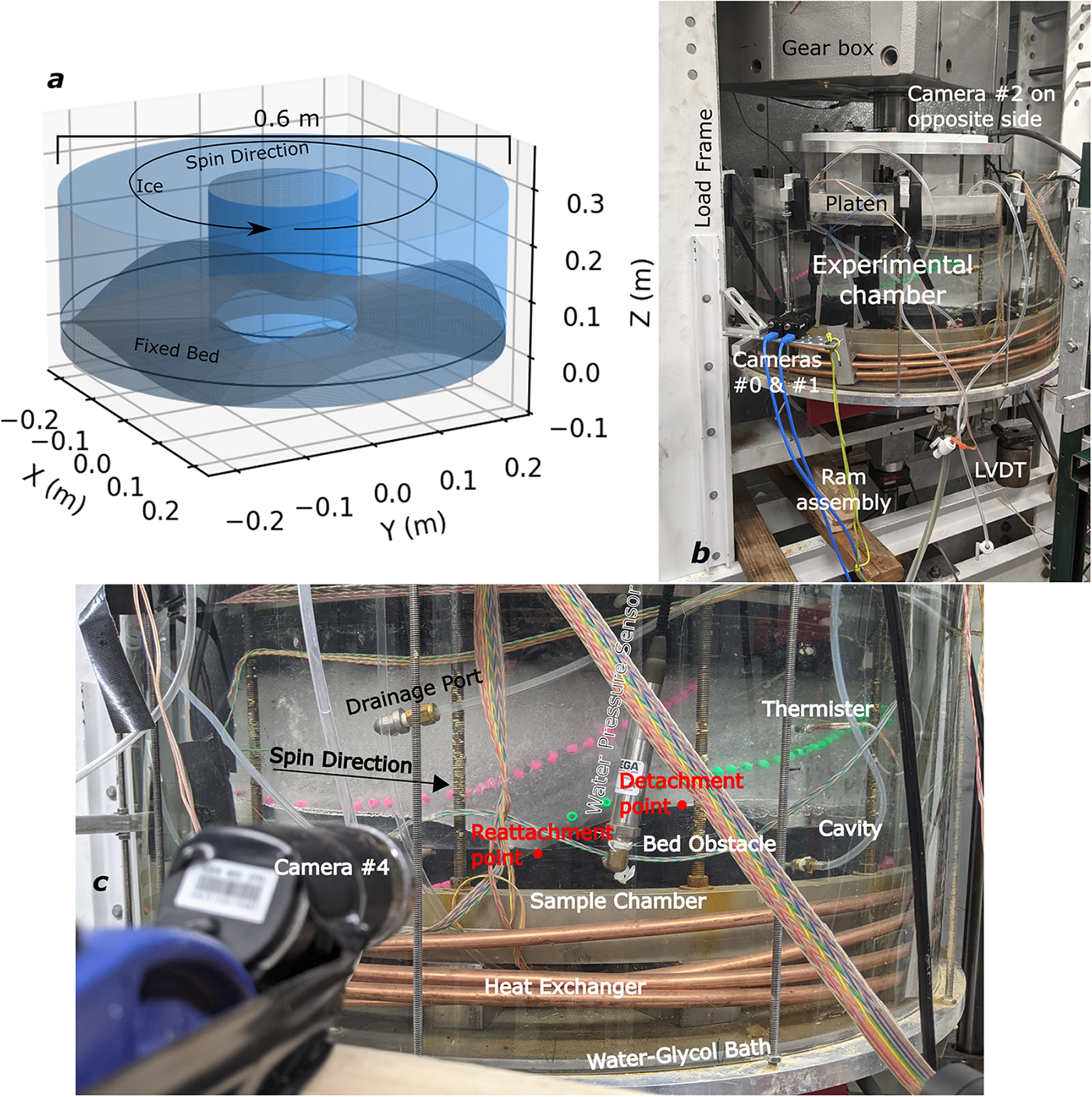
We simulated glacier slip using the University of Wisconsin–Madison Cryogenic Ring-Shear Device (UW–CRSD)—a large-diameter ring-shear device. Zoet and others (Reference Zoet, Sobol, Lord and Hansen2023) provide a comprehensive description of the UW-CRSD and its operation, so here we focus on aspects of its structure and operation relevant to our experiments: bed geometry, ice-ring construction, cavity geometry monitoring and loading profile design and execution. Figure 1 provides an overview of key components of the UW–CRSD referenced in this study. Note that the experimental chamber refers to the entire acrylic/metal housing shown in Fig. 1b, whereas the sample chamber is the vessel within the experimental chamber (Fig. 1c) that houses the ice-ring and bed (Fig. 1a).
UW-CRSD anatomy overview. (a) Scale diagram of the sample chamber contents: bed surface (gray), ice-ring (blue), and spin direction. Mean elevation of the bed is marked with a black ring. (b) Major structural components and sensors. (c) Detailed view of the experimental chamber structure, sensors and features of the bed/cavity sliding system (see text). Note: Camera numbering based on serial port indices, port #3 was unused.
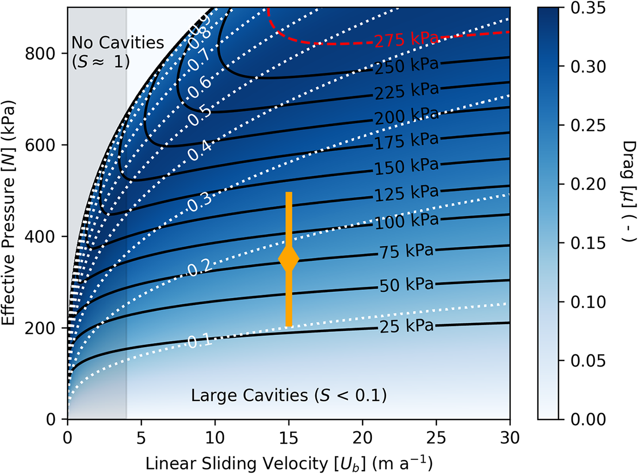
Predicted parameter space for sliding over the UW-CRSD sinusoidal bed (Table 1) using the analytic sliding rule detailed in zoet and iverson (Reference Zoet and Iverson2015) and Appendix A. Figure axes show linear slip velocities ( ${U_b}$
) and effective pressures (
${U_b}$
) and effective pressures ( $N$). Solid black contours show predicted shear stresses ( $\tau$), dotted white contours show predicted ice-bed contact fractions ( $S$) and blue shading shows predicted drag ( $\mu $; color bar). The gray shaded region shows sliding velocities below the operational limits of the UW-CRSD and the red-dashed line shows the maximum shear stress the UW-CRSD’s load frame can safely support (after Table 2). The parameter space relevant to our experiments is shown as an orange line with the average state marked as an orange diamond.
2.1.1. Rigid bed
We installed a rigid, sinusoidal bed in the UW-CRSD sample chamber (Fig. 1a) that follows design principles from prior CRSD experiments (Iverson and Petersen, Reference Iverson and Petersen2011; Zoet and Iverson, Reference Zoet and Iverson2015, Reference Zoet and Iverson2016) that allow direct comparison of experimental observations with modeled values from analytic sliding theory (Lliboutry, Reference Lliboutry1968, Reference Lliboutry1979; Kamb, Reference Kamb1987). Thus, we can compare our observations of transiently forced behaviors to those from theory and steady-state experiments for this particular bed geometry (Zoet and Iverson, Reference Zoet and Iverson2015). The bed used in our experiments is made of milled Delrin®: a polymer with a low thermal conductivity and a low friction coefficient that suppress regelation and frictional shear stress, respectively. These properties help isolate the effects of viscous deformation on system mechanics that control slip behaviors for field-scale obstacles, supporting scalability of physics constrained in the laboratory to models of real glacier systems (e.g., Cuffey and Patterson, Reference Cuffey and Patterson2010; Iverson and Petersen, Reference Iverson and Petersen2011; Zoet and Iverson, Reference Zoet and Iverson2015). We used a bed comprised of four sinusoidal obstacles, the geometry of which is summarized in Table 1.
UW–CRSD bed and sample chamber geometric parameters along the inner wall, centerline, and outer wall of the sample chamber. The centerline measurements are identical to radially averaged values of wavelength and amplitude
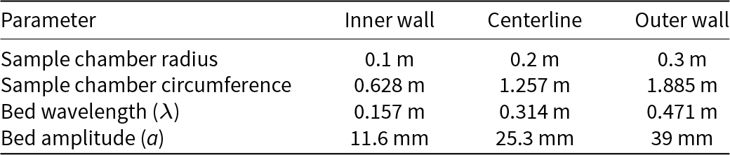
Unlike beds in prior studies, the bed used in this study had open sockets for installing mounting bolts near the crests and valleys of each obstacle. Sockets on obstacle crests were within ice-bed contact areas and provided an additional source of resisting stress. To account for the effect of these sockets, we constrained a new correction factor for measured shear stresses not included in established CRSD protocols (see Section 3.2).
2.1.2. Ice-ring
After installing the sinusoidal bed, we constructed an ice-ring with an average height of 25 cm in a series of 5 cm layers. Layers consisted of crushed, deionized water-ice that were flooded with near-freezing deionized water and allowed to freeze in place at the ambient laboratory temperature (approximately −10°C). Prior to making the final ice layer, we installed strain markers (beads) near the outer wall of the sample chamber and froze these in place with additional deionized water (see Figs 1b, c). Immediately after flooding the final layer, we lowered the platen into contact with the ice-ring, sealing the sample chamber and allowing the Delrin® teeth of the upper platen to freeze into the top of the ice-ring (Fig. 1b). Like the bed, the use of Delrin® for the platen teeth provides better coupling between the ice-ring and the rotating platen that drove radial shearing at a specified angular velocity ( $\omega $) throughout the study.
2.1.3. Operation and data acquisition
We applied vertical pressures to the contents of the sample chamber using a computer controlled ISCO pump connected to a hydraulic ram (Fig. 1b). The ram adjusted the vertical position of the experimental chamber, and a pressure transducer in the ram assembly measured the vertical force applied by the ram. Control systems continuously monitored data from the pressure transducer and adjusted the vertical position of the ram and experimental chamber to maintain a prescribed vertical force on the contents of the sample chamber. Prior CRSD studies maintained a constant vertical force for the entirety of each experiment. In our experiments, we imposed oscillatory loading profiles to emulate cycles in subglacial effective pressure ( $N$), calculating the vertical pressure ( $P_V$) as the applied force divided by the cross-sectional area of the sample chamber and subtracting measured water pressure ( $P_W$) in the sample chamber ( $N=P_V-P_W$). We corrected vertical force measurements for the mass of the experimental chamber and its contents prior to calculating $P_V$. As the ice-ring melted, water was passively evacuated at near-atmospheric pressures via drainage ports in the bottom and sides of the sample chamber. Evacuated water was retained in buckets attached to the outside of the experimental chamber, maintaining the cumulative mass supported by the ram throughout the study. Water pressures in the sample chamber were monitored with two water pressure transducers (Fig. 1c), and we used the average of these data to calculate $N$.
$N$.
As the platen rotated the ice-ring at a uniform angular velocity, resisting forces generated through slip processes were measured using a custom torque transducer fixed to the base of the experimental chamber (Fig. 1b). Torques were initially corrected for resisting forces provided by the gasket that seals the sample chamber at the platen (after Zoet and Iverson, Reference Zoet and Iverson2015; Zoet and others, Reference Zoet, Sobol, Lord and Hansen2023) and converted to a shear stress. We subsequently estimated corrections for resistance provided by the mounting sockets using  $\tau $ observations and modeled values during geometrically confirmed steady-state periods. We then calculated drag from calibrated measurements of $N$ and ${{\tau }}$ ( ${{\mu }} = \,{{\tau }}/\,N$).
Changes in cavity geometry can produce changes in vertical separation of a glacier and its bed (e.g., Andrews and others, 2014; Zoet and others, Reference Zoet, Iverson, Andrews and Helanow2022). To continuously monitor changes in ice-bed separation during our experiments, we used a linear vector displacement transducer (LVDT) attached to the exterior of the experimental chamber (Fig. 1b). During our experiments, the LVDT was occasionally reset to keep the sensor within its dynamic range. These adjustments were manually corrected in the data to produce a continuous time series of the relative vertical position of the experimental chamber throughout this study. Additionally, time-lapse cameras were deployed around the UW-CRSD to directly observe changes in cavity geometries (Figs 1b, c).
Transducer measurements for vertical forces, torques and water pressures were recorded every 15 s, and photos were taken by all cameras every minute (Figs 1b, c). We filtered out occasional, short-duration spikes (lasting less than four samples) in time series associated with episodic delays in loading ram response. All but one of these spikes occurred outside the timing of our loading experiments, apart from a spike at the start of the 24 h oscillation experiment (see supplementary Figure S1 and text).
2.2. Experiment design
2.2.1. Steady-state theory
The steady-state experimental observations presented in Zoet and Iverson (Reference Zoet and Iverson2015) demonstrated a ‘double-valued’ drag relationship for glacier slip over sinusoidal bedforms consistent with analytic theory for a range of slip velocities (Lliboutry, Reference Lliboutry1968, Reference Lliboutry1979; Kamb, Reference Kamb1987). This experimentally constrained double-valued drag law states that as cavities nucleate and dilate in response to rising  $U_b$, drag ( $\mu $) provided by the system increases and therefore ${{\tau }}$ increases without a change in $N$. Past a certain threshold dictated by the relative geometry of cavities and bed obstacles—parameterized as the ice-bed contact length fraction $S$—further cavity dilation from subsequent increases in $U_b$ result in decreasing ${{\mu }}$. Thus, ${{\tau }}$ decreases without a change in $N$ as $U_b$ continues to rise past this geometrically defined inflection point. Comparable decreases in $U_b$ allow viscous contraction of cavities, which the double-valued drag theory indicates should result in a reciprocal evolution of $\mu $ and ${{\tau }}$ along the same path. This is an expression of the underlying assumption in analytic theory that at any point in the system’s evolution, the cavity geometry is in a steady-state configuration relative to the current $U_b$.
Whereas cavities can also nucleate and dilate in response to decreasing  $N$, analytic theory suggests that a double-valued drag relationship should also apply for $N$ modulated systems (i.e., water pressure modulation). Using the system of equations from Zoet and Iverson (Reference Zoet and Iverson2015) (recapitulated in Appendix A), the geometry of the UW-CRSD sample chamber and bed (Table 1) and rheologic parameters for temperate ice constrained in Zoet and Iverson (Reference Zoet and Iverson2015), we modeled the parameter space for $N$,
$N$,  $U_b$, ${{\tau }}$, ${{\mu }}$ and $S$ shown in Fig. 3. Using these modeled values, we identified a region of parameter space that avoids the inflection point between increasing and decreasing ${{\mu }}$, encompasses a range of $N$ values consistent with borehole observations near the Greenland Ice-Sheet margin (Andrews and others, 2014) and falls within the operational limits of the UW-CRSD (grayed-out areas in Fig. 3; summarized in Table 2). Subsequent references to modeled values are denoted with a ‘calc’ superscript (e.g., $\tau^\text{calc}$) throughout this report. All parameters appearing in this study (and sub-/superscripted versions thereof) are summarized in Table B1 of Appendix B.
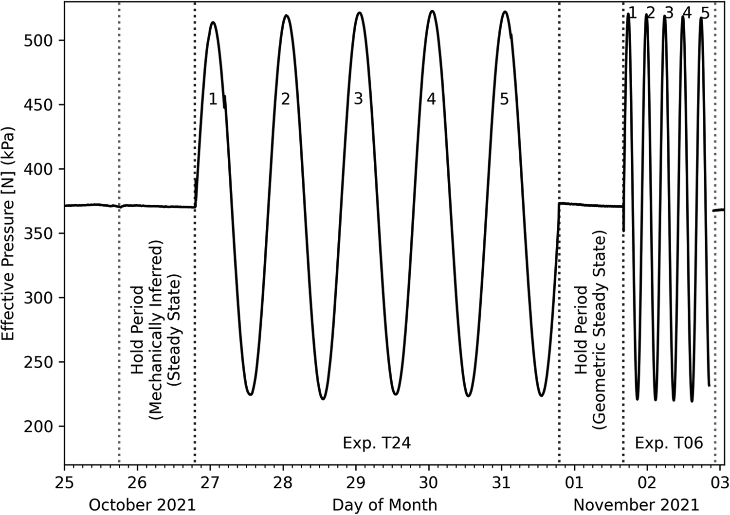
Observed effective pressures  $(N)$ for Exp. T24, Exp. T06 and intervening hold periods. cycle numbers within experiments are labeled and the nature of hold periods’ steady-state are annotated (see text). hold period and experiment start/stop times are marked with vertical dotted lines.
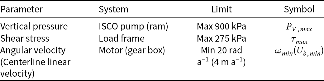
Operational limits of relevant UW–CRSD control systems and superstructure
2.2.2. Loading profile design
We targeted an average vertical pressure ( $P_V$) of 350 kPa for all our experiments and a pressure oscillation amplitude ( $P_A$) of 140 kPa. These parameters approximate conditions at the bed of a 400 m-thick glacier at 90% flotation pressure (hydrologic head height of 330 m) experiencing a 15.5 m head oscillation amplitude—roughly twice the amplitude observed by Andrews and others (2014) in boreholes accessing cavity networks and five times smaller than their observations in boreholes in nearby moulins. Correcting for observed ${P_W}$, imposed effective pressure cycles were measured as
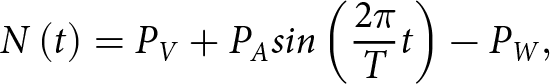 \begin{equation}N\left(t\right)=P_V+P_Asin\left(\frac{2\pi}Tt\right)-P_W,\end{equation}
 with oscillation period  $T$ and observation times $t$. Observed ${P_W}$ values rarely exceeded 3 kPa (1% of ${P_V}$), with one notable excursion reaching 18 kPa associated with the $P_V$ spike at the start of the 24 h cycling experiment (supplement, Fig. S1). To assess a broader range of cavity geometries during this experiment— $S \in \left[ {0.1,0.3} \right]$—we prescribed a centerline slip velocity ( $U_b$) of 15 m a−1 (angular velocity of 75 rad a−1) instead of a $U_b$ value observed at the Greenland Ice-Sheet margin (60–160 m a−1; Andrews and others, 2014). This still permitted all expected $N\left( t \right)$ values to fall into a domain where $N$ and $\mu $ covary (Fig. 3; orange bar). Following a spin-up period, our first experiment used $T$ = 24 h (Exp. T24) to simulate the dominant forcing period for surface-melting forced glacier systems. Our second experiment used $T$ = 6 h (Exp. T06) to investigate the effect of shorter forcing periods on slip mechanics and cavity geometries. We attempted a third experiment with $T$ = 96 h starting 24 h after the end of Exp. T06, but it was incomplete due to operational issues (i.e., loss of power/pressure in the ram) (see Fig. S1). As such, we focus on results from experiments T24 and T06 in this study. Raw data from experiment T96 are included in the repository (see Data availability statement) and interested readers are directed to Stevens (Reference Stevens2022) for further information on this third experiment (Exp. T96).
Ice dynamics modeling by Law and others (Reference Law, Christoffersen, MacKie, Cook, Haseloff and Gagliardini2023) suggests most slip occurs with ice at pressure melting temperatures (i.e., temperate ice). To emulate these conditions in the laboratory, the UW-CRSD is housed in a walk-in freezer that maintains temperatures to within 1°C of target values and the sample chamber is enveloped in a temperature regulation system that maintains temperatures to within 0.01°C of target values. The temperature regulation system comprises a circulating water–glycol bath that fills the outer volume of the experimental chamber and uses computer-controlled heat exchangers and glass bead thermistors imbedded in the sample chamber walls to monitor and regulate the sample chamber’s temperature (Fig. 1c). The pressure melting temperature ( $\Theta_{PMT}$) is calculated as
 \begin{equation}{\Theta _{{{PMT}}}}\left( {\rm{N}} \right) = {\Theta _{TP}} - \gamma \left( {{\rm{N}} - {P_{TP}}} \right)\end{equation}
with the triple-point temperature ( $\textstyle\Theta_{TP}$= 273.15 K) and pressure ( ${P_{TP}}$
= 611.73 Pa) for pure water and the Clausius–Clapeyron parameter (
${P_{TP}}$
= 611.73 Pa) for pure water and the Clausius–Clapeyron parameter ( $\gamma $ = 9.8 × 10⁻⁸ K Pa−1; e.g., Hooke, Reference Hooke2005) for pure, air-saturated water. Before initiating slip in the experiment, we raised the temperature in the sample chamber to −0.034°C ( $\Theta_{PMT}$ for $N$ = 350 kPa) and maintained this temperature within control system tolerances for the remainder of the experiment.
2.2.3. Experiment spin-up and execution
We initialized our experiment with a ‘spin-up’ period to develop large, steady-state cavities ( $S \approx 0.2$) under a low applied pressure ( $P_V$
$P_V$  $ \approx $ 180 kPa) to expedite cavity growth and allow longer experiment run-time before the ice-ring melted to an inoperable thickness. We increased ${P_V}$ to 350 kPa and drove the system to steady-state according to established methods, defined by sustained ${{\tau }}$ values that do not vary by more than 1% for at least 6 h (Zoet and Iverson, Reference Zoet and Iverson2015, Reference Zoet and Iverson2016; Zoet and others, Reference Zoet, Iverson, Andrews and Helanow2022, Reference Zoet, Sobol, Lord and Hansen2023). We refer to this as a ‘mechanically inferred steady-state’. Exp. T24 started without a target number of oscillations, rather we continued oscillations until we observed nearly identical ${{\tau }}$ responses for two successive oscillations: cycles 4 and 5. After Exp. T24, we held $P_V$ at 350 kPa for 24 h while maintaining the slip rate to allow the system to return to steady-state conditions and then initiated Exp. T06, which we ran for five cycles. Observed $N$ values during both experiments and hold periods are shown in Fig. 3 and imposed $P_V$ and observed $P_W$ values are included in the supplement (Fig. S1). We also reproduce ${P_V}$
and
${P_V}$
and  $N$ time series in Figs 5 and 6 for the time periods of Exp. T24 and T06, respectively.
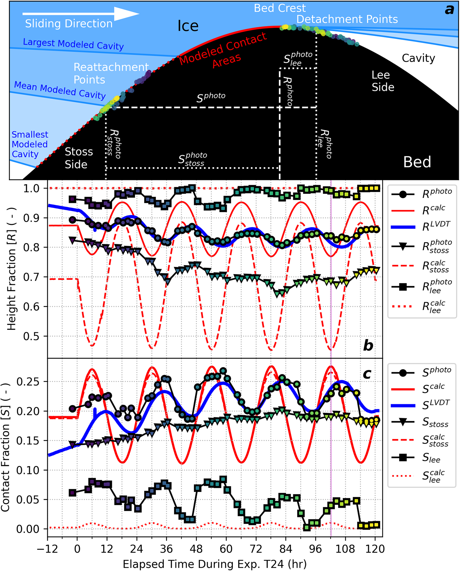
Cavity geometry evolution during Exp. T24. (a) Spatial distribution of photo-derived detachment and reattachment points overlain on a bed obstacle (black). The range of cavity geometries predicted from modeling are shown in blue and annotated, and the range of contact surfaces are shown in red. The minimum contact surface is shown as a solid red line, whereas regions over which model predictions oscillate on the stoss and lee are shown as dotted lines. (b–c) Time series of photo-derived, LVDT-derived, and model estimates of (b) average cavity height ( $R$) and (c) ice-bed contact length ( $S$). measurements of $S$ and $R$ from photos are illustrated and annotated in (a) and correspond to the time shown as a magenta line in (b–c). Photo-derived measurements are color-coordinated in all subplots to convey their timing.
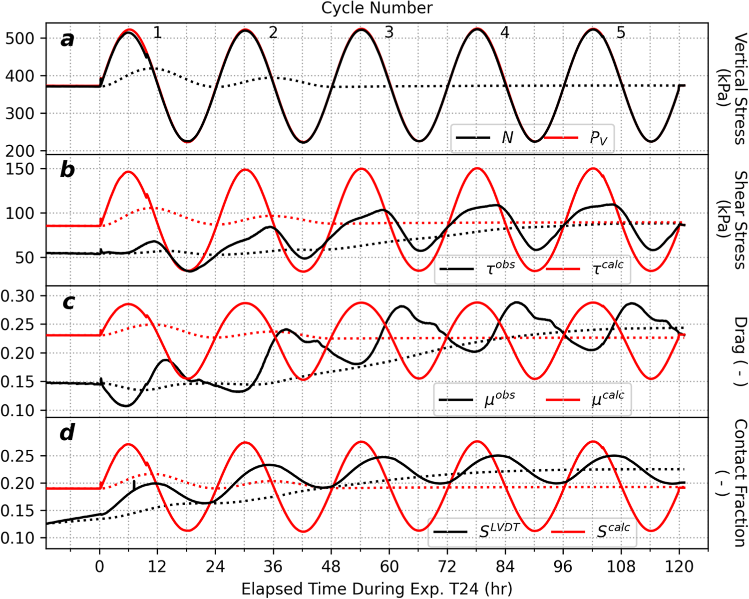
Time series of observed (black lines) and modeled/applied (red lines) mechanical parameters for Experiment T24. (a) effective stress ( $N$) and applied vertical stress ( ${P_V}$
), (b) shear stress (
${P_V}$
), (b) shear stress ( ${{\tau }}$), (c), drag ( ${{\mu }}$) and (d) ice-bed contact fraction ( $S$). Dotted lines are the 48 h moving averages of observed (black) and modeled (red) values. Cycle numbers are noted in (a).
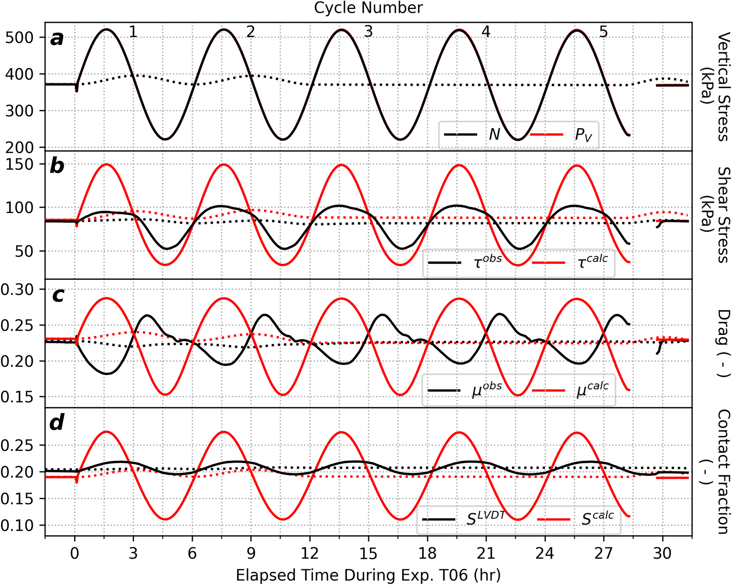
Time series of observed (black lines) and modeled/applied (red lines) mechanical parameters for Eexperiment T06. (a) Effective stress ( $N$) and applied vertical stress ( ${P_V}$
), (b) shear stress (
${P_V}$
), (b) shear stress ( ${{\tau }}$), (c), drag ( $\mu$) and (d) ice-bed contact fraction ( $S$). Dotted lines are 12 h moving averages of observed (black) and modeled (red) values. Cycle numbers are noted in (a). The gap in each figure arose from a logging gap for the pressure and torque transducers.
2.3. Cavity geometry monitoring
Ice-bed contact geometry plays a central role in hard-bedded sliding theory, with the size and slope of ice-bed contact areas modulating the resisting stresses provided by a rigid obstacle (Lliboutry, Reference Lliboutry1968, Reference Lliboutry1979; Kamb, Reference Kamb1987; Zoet and Iverson, Reference Zoet and Iverson2015; Helanow and others, Reference Helanow, Iverson, Woodard and Zoet2021). Direct observation of cavity and ice-bed contact area geometries is exceedingly difficult in subglacial environments, so changes in ice-bed separation (the change in cavity height/volume) are typically used as a proxy for changes in ice-bed contact size (Iken and Bindschadler, Reference Iken and Bindschadler1986; Andrews and others, 2014; Zoet and Iverson, Reference Zoet and Iverson2015, Reference Zoet and Iverson2016; Zoet and others, Reference Zoet, Iverson, Andrews and Helanow2022). To generalize system geometries across scales, analytic theory normalizes contact areas by a characteristic length of bed obstacles ( $\lambda $, here), yielding a nondimensionalized contact length parameter ( $S$).
$S$).  $S$ is a function of the lateral positions of where the cavity lifts off the bed (the detachment point, Fig. 1c) and where it rejoins the bed (the reattachment point, Fig. 1c).
In analytic theory,  $S$ is related to ice-bed separation by the geometry of a cavity’s roof and the geometry of the bed (Appendix A; Zoet and Iverson, Reference Zoet and Iverson2015). Measurements from the LVDT contain a record of changes in average ice-bed separation due to changes in cavity volume, so taking the average elevation from modeled cavity roof geometries should emulate LVDT measurements arising from changes in cavity geometry. Numerical analysis showed that the arithmetic mean of a modeled cavity roof profile was equivalent to average elevation of the modeled detachment and reattachment points. As such, we used the horizontal and vertical positions of the detachment and reattachment points to define $S$ and a comparable, nondimensionalized parameter for cavity height ( $R$). We define $R$ as the average cavity height normalized by the characteristic height of bed obstacles (twice the bed amplitude, $a$, in Table 1). By using detachment and reattachment points to parameterize cavity geometries, we can also use point measurements from time-lapse photos to directly compare observed cavity geometries, LVDT-derived geometries and modeled geometries.
We derived  $S$ and $R$ from time-lapse images by manually picking the positions of cavity detachment points $(\left\{ {{x_d},\,{y_d}} \right\})$
, reattachment points
$(\left\{ {{x_d},\,{y_d}} \right\})$
, reattachment points  $(\left\{ {{x_r},\,{y_r}} \right\})$
, obstacle crests
$(\left\{ {{x_r},\,{y_r}} \right\})$
, obstacle crests  $(\left\{{x_c} = 0, {y_c} = 2a\right\})$ and static reference points (e.g., drainage ports; Fig. 1c). The full sequence of time lapse images for Exp. T24 are provided in Movies S1 through S3 (supplement), but due to the labor-intensive nature of manually picking point data in raw images, we chose to analyze 50 frames from cameras #2 and #4 (Figs 1b, c) that coincided with extremum in stresses, drag and LVDT cycles throughout Exp. T24. In addition, we analyzed images from the hold periods before and after Exp. T24 to constrain a reference, steady-state geometry. We then used the reference points and known geometry of the bed to reproject raw images and picked points into a flattened reference frame using a linear transformation algorithm provided with the QGIS GeoReferencer plugin (QGIS Association, 2024). Finally, we applied small, translational (<1 mm) and rotational (<2°) adjustments on picked data to align reference points across images and cameras. Photo-derived estimates of scaled geometric parameters ( ${R^{photo}}$
and
${R^{photo}}$
and  ${S^{photo}}$
) as
${S^{photo}}$
) as
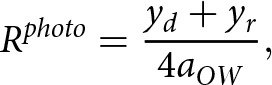 \begin{equation}{R^{photo}} = {{{y_d} + {y_r}} \over {4{a_{OW}}}},\end{equation}
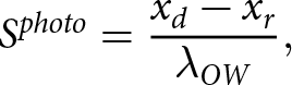 \begin{equation}{S^{photo}} = {{{x_d} - {x_r}} \over {{\lambda _{OW}}}},\end{equation}
 using the amplitude and wavelength of the bed along the outer wall of the sample chamber ( ${a_{OW}}$
and
${a_{OW}}$
and  ${\lambda_{OW}}$
, respectively; Table 1).
${\lambda_{OW}}$
, respectively; Table 1).
Measurements from the LVDT record the summation of ice-ring melting and changes in the average height of cavities. We corrected LVDT measurements ( ${y^{LVDT}}$
) at times (
${y^{LVDT}}$
) at times ( $t$) for the average melting rate of the ice-ring during each experiment ( $m$) and calibrated them to a photo-derived reference geometry ( ${R^{photo}}$
) at the time of a steady-state cavity configuration (
${R^{photo}}$
) at the time of a steady-state cavity configuration ( ${t_0}$
).
${t_0}$
).  ${R^{LVDT}}$
is therefore calculated as
${R^{LVDT}}$
is therefore calculated as
 \begin{equation}{R^{LVDT}}\left( t \right) = {{{y^{LVDT}}\left( t \right) - m\left( {t - {t_0}} \right) - {y^{LVDT}}\left( {{t_0}} \right)} \over {2{a_{CL}}}} + {R^{photo}}\left( {{t_0}} \right),\end{equation}
with the average (centerline) bed obstacle amplitude ( ${a_{CL}}$
; Table 1). We then approximated a function relating
${a_{CL}}$
; Table 1). We then approximated a function relating  $S$ and $R$ using analytic theory to estimate a calibrated, fractional contact area from LVDT observations ( ${S^{LVDT}}$
). Modeled values for
${S^{LVDT}}$
). Modeled values for  $S$ and were calculated using the system of equations in Appendix A. Values of ${S^{calc}}$
were calculated using Eqn A8 and centerline geometries (Table 1), and
${S^{calc}}$
were calculated using Eqn A8 and centerline geometries (Table 1), and  ${R^{calc}}$
values were calculated as the mean roof elevation
${R^{calc}}$
values were calculated as the mean roof elevation
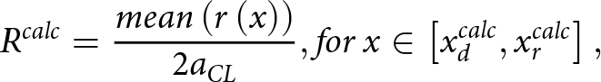 \begin{equation}{R^{calc}} = {{mean\left( {r\left( x \right)} \right)} \over {2{a_{CL}}}}, for\, x \in \left[ {x_d^{calc},x_r^{calc}} \right],\end{equation}
with  $r\left( x \right)$ from Eqn A2 for positions $x$ that lie at or above the modeled bed (Eqn A1).
As indicated by Eqn 2, the melting temperature (and thus melting rate) at ice-bed contacts should vary linearly with  $N$ during oscillatory loading experiments. Whereas we applied symmetric, periodic $N$ cycles in both experiments, the average slope of the LVDT data across multiple loading cycles should reflect the average melting rate across those cycles. To estimate the long-term-average $m$ for our experiments, we only used data from complete cycles that exhibited highly similar $\tau $ cycles to estimate $m$ (cycles 4–5 in Exp. T24 and 2–5 in Exp. T06). This assumes that the highly similar ${{\tau }}$ cycles arise from highly similar cycles in cavity/contact geometry. Within cycles, times with relatively higher $N$ should favor enhanced melting at ice-bed contacts and vice versa. Therefore, the amplitudes of ${R^{LVDT}}$
corrected with the average melting rate may over-estimate the range of cavity heights due to modulation of within cycles not accounted for by this melt correction method.
${R^{LVDT}}$
corrected with the average melting rate may over-estimate the range of cavity heights due to modulation of within cycles not accounted for by this melt correction method.  ${S^{LVDT}}$
inversely varies with
${S^{LVDT}}$
inversely varies with  ${R^{LVDT}}$
, so unaccounted for melting-rate modulation within cycles would lead to
${R^{LVDT}}$
, so unaccounted for melting-rate modulation within cycles would lead to  ${S^{LVDT}}$
under-estimating the true range of ice-bed contact lengths during our experiments.
${S^{LVDT}}$
under-estimating the true range of ice-bed contact lengths during our experiments.
Through direct observation, we can also assess a key assumption present in analytic theory: that ice-bed contact areas on the stoss (up-flow) side of bed obstacles provide resisting stresses, and therefore changes in stoss contact area explain all observed changes in drag and resisting stresses provided by ice-bed contacts. As a corollary, analytic theory indicates lee contact areas remain small and do not contribute appreciably to the mechanical response of the system. To inspect these features, we define stoss- and lee-side contact areas derived from photos as
 \begin{equation}S_{stoss}^{photo} = {{{x_c} - {x_r}} \over {{\lambda _{OW}}}},\end{equation}
 \begin{equation}S_{lee}^{photo} = {{{x_d} - {x_c}} \over {{\lambda _{OW}}}},\end{equation}
 \begin{equation}R_{stoss}^{photo} = {{{y_c} - {y_r}} \over {2{a_{OW}}}},\end{equation}
 \begin{equation}R_{lee}^{photo} = {{{y_c} - {y_d}} \over {2{a_{OW}}}}.\end{equation} $S$ and $R$ and their geometric relationship to bed obstacle and cavity geometries is provided in Fig. 4a, including component measurements on lee and stoss sides of an obstacle.
3. Results
3.1. Cavity geometries
Our photo-derived observations of cavity geometries during Exp. T24 are shown in Fig. 4 and compared to LVDT- and model-derived estimates. Figure 4a shows the spatial distribution of photo-derived cavity detachment and reattachment points overlain on the range of cavity and contact area geometries predicted by analytic theory. We found that observed detachment points ranged over a much wider section of the lee side of the obstacle than predicted by modeling. Similarly, observed reattachment points raged over a much narrower section of the stoss side of the obstacle relative to model predictions. As Exp. T24 progressed, both the detachment and reattachment points migrated toward an average position generally consistent with model predictions for average  $N$ (and ${U_b}$
) in this experiment (marker colors progressing from dark to light in Fig. 4a).
${U_b}$
) in this experiment (marker colors progressing from dark to light in Fig. 4a).
Figure 4b shows the temporal evolution of  $R$ estimates from photos, LVDT measurements and modeling, and includes component estimates of $R$ (lee and stoss) from photos and modeling. ${R^{photo}}$
and
${R^{photo}}$
and  ${R^{LVDT}}$
tracked closely with one another indicating that our correction factors applied to LVDT data reasonably approximated the true, average height of cavities (Eqn 4). Both
${R^{LVDT}}$
tracked closely with one another indicating that our correction factors applied to LVDT data reasonably approximated the true, average height of cavities (Eqn 4). Both  ${R^{photo}}$
and
${R^{photo}}$
and  ${R^{LVDT}}$
oscillated in a narrower range of values compared to
${R^{LVDT}}$
oscillated in a narrower range of values compared to  ${R^{calc}}$
and have long-term, increasing trends over cycles 1–3 and steady mean values during cycles 4 and 5. This intercycle trend supports our interpretation of stabilizing mean cavity geometries during these later cycles provides further support for our melt correction method (Eqn 4 and text). Oscillations in
${R^{calc}}$
and have long-term, increasing trends over cycles 1–3 and steady mean values during cycles 4 and 5. This intercycle trend supports our interpretation of stabilizing mean cavity geometries during these later cycles provides further support for our melt correction method (Eqn 4 and text). Oscillations in  ${R^{photo}}$
had relatively even contributions from variations in
${R^{photo}}$
had relatively even contributions from variations in  $R_{lee}^{photo}$
and
$R_{lee}^{photo}$
and  $R_{stoss}^{photo}$
reflecting a general observation that the entire cavity roof raised and lowered during
$R_{stoss}^{photo}$
reflecting a general observation that the entire cavity roof raised and lowered during  $N$ cycles (see movies in supplement; Mov. S1–S3).
Figure 4c shows the temporal evolution of  $S$ estimates from photos, LVDT data, and modeling and component estimates. We found that ${S^{photo}}$
and
${S^{photo}}$
and  ${S^{LVDT}}$
tracked together well for cycles 3–5, with under-estimating
${S^{LVDT}}$
tracked together well for cycles 3–5, with under-estimating  $S^{photo}$ during cycles 1 and 2. Contrary to model predictions, we observed that $S_{lee}^{photo}$
accounted for most of the variability in
$S_{lee}^{photo}$
accounted for most of the variability in  ${S^{photo}}$
within cycles, whereas
${S^{photo}}$
within cycles, whereas  $S_{stoss}^{calc}$
accounted for most of the variability in
$S_{stoss}^{calc}$
accounted for most of the variability in  ${S^{calc}}$
. remained relatively stable within cycles, instead displaying two distinct long-term trends: a linear increase across cycles 1–3 and a steady configuration across cycles 4 and 5. Our observations call the assumption of minimally important lee contact area dynamics into question.
${S^{calc}}$
. remained relatively stable within cycles, instead displaying two distinct long-term trends: a linear increase across cycles 1–3 and a steady configuration across cycles 4 and 5. Our observations call the assumption of minimally important lee contact area dynamics into question.
In summary, we found the following differences between observed cavity geometries and model predictions:
1) Observed cavity shapes oscillate in a narrower range compared to steady-state model predictions.
2) Observed cavity geometry changes lagged model predictions by 4 h.
3) Observed contact-area oscillations primarily arose from changes in the size of the lee contact area within cycles and from stoss contact areas across cycles.
Despite these differences, analytic theory closely matches cavity geometries observed at the end of Exp. T24 suggesting that the system oscillated about a steady-state configuration close to model predictions. Additionally, we found that LVDT-derived estimates of cavity geometries were a reasonable approximation for photo-derived values, supporting the use of LVDT measurements as a proxy for ice-bed contact size with appropriate correction factors. The selection of these correction factors is presented in the next section alongside our measurements of the system’s mechanical response to transient forcing.
3.2. Empirical correction factors
Photo-derived cavity geometry measurements closely matched modeled equivalents from analytic theory at the end of Exp. T24 (Figs 4a–c), which we interpret as a geometrically constrained steady-state (labeled in Fig. 3). As such, we used geometric and mechanical measurements from the hold period following Exp. T24 to calibrate LVDT measurements and estimate a correction factor for added resisting stresses arising from mounting bolt sockets. These correction factors are summarized in Table 3 and described below.
Individual empirical correction factors for LVDT measurements relevant to Eqn 4
We used the last  ${R^{photo}}$
measurement in Fig. 4b to calibrate LVDT estimates of
${R^{photo}}$
measurement in Fig. 4b to calibrate LVDT estimates of  $R$ and $S$ (Eqn 4), and geometric and mechanical measurements from averaged $N$ and ${U_b}$
values observed in the 24 h hold period between Exp. T24 and Exp. T06 to model predicted shear stress for this cavity geometry (
${U_b}$
values observed in the 24 h hold period between Exp. T24 and Exp. T06 to model predicted shear stress for this cavity geometry ( ${\tau^{calc}}$
; Eqn A5). Modeled values used the same flow-law exponent (
${\tau^{calc}}$
; Eqn A5). Modeled values used the same flow-law exponent ( $n$ = 3) and effective viscosity ( $B$ = 63 MPa a−1/3) as Figs 3 and 4 and analyses in Zoet and Iverson (Reference Zoet and Iverson2015). We then attributed the difference between ${\tau^{calc}}$
and observed shear stresses corrected for resistance from the platen gasket (
${\tau^{calc}}$
and observed shear stresses corrected for resistance from the platen gasket ( $\tau ^{\prime}$) to the additional resistance arising from the mounting bolt sockets in the bed, yielding a correction factor
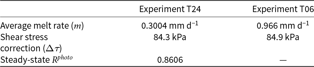
  ${{\Delta }}\tau $ = 84.3 kPa. Changing cavity geometries throughout both experiments and hold periods did not expose or envelop additional sockets, so we hypothesized that the enveloped sockets provided a relatively uniform shear stress enhancement throughout our experiments. To test this hypothesis, we repeated this analysis with data from the 24 h hold after the end of Exp. T06 and found a nearly identical value: ${{\Delta }}\tau $ = 84.9 kPa. Thus, we applied a uniform correction of ${{\Delta }}\tau $ = 84.6 kPa to all shear stress measurements, yielding the observed shear stresses ( ${\tau ^{obs}} = \tau ^{\prime} - \Delta \tau $
) in Figs 5b and 6b. We then calculated observed drag as:
${\tau ^{obs}} = \tau ^{\prime} - \Delta \tau $
) in Figs 5b and 6b. We then calculated observed drag as:  ${\mu ^{obs}} = {\tau ^{obs}}/{N^{obs}}$
(Figs 5c and 6c). The estimate for
${\mu ^{obs}} = {\tau ^{obs}}/{N^{obs}}$
(Figs 5c and 6c). The estimate for  $m$ in Exp. T06 used LVDT data from cycles 2–5, where ${\tau ^{{\rm{obs}}}}$
cycles are highly similar. We found
${\tau ^{{\rm{obs}}}}$
cycles are highly similar. We found  $m$ = 0.966 mm d−1, which is still within the range of correction factors estimated across experiments reported in Zoet and Iverson (Reference Zoet and Iverson2015) despite its threefold difference relative to $m$ from Exp. T24 (Table 3).
3.3. System evolution
3.3.1. Experiment T24
The mechanical response of this system to 24 h  $N$ cycles shown in Fig. 5 displays a rich variety of features that diverge from analytic theory predictions, but also shows long-term trends that agree with analytic theory. Effective pressures closely tracked with applied vertical pressures (Fig. 5a), with a small deviation during cycle 1 associated with a spike in ${P_V}$
and
${P_V}$
and  ${P_W}$
. This spike did not appreciably impact the form of the forcing during Exp. T24 or the recorded system responses. We found that
${P_W}$
. This spike did not appreciably impact the form of the forcing during Exp. T24 or the recorded system responses. We found that  ${\tau^{obs}}$
oscillated in a narrower range relative to
${\tau^{obs}}$
oscillated in a narrower range relative to  ${\tau^{calc}}$
, but
${\tau^{calc}}$
, but  ${\tau^{obs}}$
remained within the predicted range of
${\tau^{obs}}$
remained within the predicted range of  ${\tau^{calc}}$
values throughout the experiment (Fig. 5b).
${\tau^{calc}}$
values throughout the experiment (Fig. 5b).  ${\tau^{obs}}$
exhibited systematic asymmetry within cycles characterized by protracted peaks and narrowed troughs, with peak
${\tau^{obs}}$
exhibited systematic asymmetry within cycles characterized by protracted peaks and narrowed troughs, with peak  ${\tau^{obs}}$
aligning with peaks in
${\tau^{obs}}$
aligning with peaks in  ${S^{LVDT}}$
, rather than peaks in
${S^{LVDT}}$
, rather than peaks in  $N$ (Figs 5a, b and d). To inspect the intercycle average system response, we calculated the 48 h rolling average of observed and modeled time series (dotted lines in Fig. 5). ${\tau^{obs}}$
(dotted black line in Fig. 5b) rose across cycles 1–3 and converged with the comparable rolling average of
${\tau^{obs}}$
(dotted black line in Fig. 5b) rose across cycles 1–3 and converged with the comparable rolling average of  ${\tau^{calc}}$
during cycles 4 and 5, indicating that the resisting stresses provided by the system converged with predicted values on intercycle timescales, with
${\tau^{calc}}$
during cycles 4 and 5, indicating that the resisting stresses provided by the system converged with predicted values on intercycle timescales, with  ${\tau^{obs}}$
oscillating about this quasi-steady-state mean within each cycle. Observed drag (
${\tau^{obs}}$
oscillating about this quasi-steady-state mean within each cycle. Observed drag ( ${\mu^{obs}}$
) oscillated with a complex pattern in a narrower range compared to predicted drag (
${\mu^{obs}}$
) oscillated with a complex pattern in a narrower range compared to predicted drag ( ${\mu ^{{\rm{calc}}}}$
) and systematically lagged
${\mu ^{{\rm{calc}}}}$
) and systematically lagged  ${\mu^{calc}}$
cycles by 12 h (Fig. 5c). Unlike
${\mu^{calc}}$
cycles by 12 h (Fig. 5c). Unlike  ${\tau^{obs}}$
, the 48 h rolling average of
${\tau^{obs}}$
, the 48 h rolling average of  ${\mu ^{{\rm{obs}}}}$ was higher than the rolling average of ${\mu^{calc}}$
by 7.7%.
${\mu^{calc}}$
by 7.7%.  ${S^{LVDT}}$ showed similar lags and enhancements compared to ${S^{calc}}$ (Fig. 5d), with ${S^{LVDT}}$
oscillations lagging
${S^{LVDT}}$
oscillations lagging  ${S^{calc}}$
by 4 h and an enhancement of the rolling average
${S^{calc}}$
by 4 h and an enhancement of the rolling average  ${S^{LVDT}}$
of 17.0% relative to the rolling average of
${S^{LVDT}}$
of 17.0% relative to the rolling average of  ${S^{calc}}$
. These lags are consistent with relationships reported in Zoet and others (Reference Zoet, Iverson, Andrews and Helanow2022) for a comparable system forced by
${S^{calc}}$
. These lags are consistent with relationships reported in Zoet and others (Reference Zoet, Iverson, Andrews and Helanow2022) for a comparable system forced by  ${U_b}$
transients with a dominant period of 24 h.
${U_b}$
transients with a dominant period of 24 h.
3.3.2. Experiment T06
The responses of this sliding system to 6 h cycles in  $N$ (Exp. T06) shown in Fig. 6 share many features with observations from Exp. T24 (Fig. 5). The $N$ forcing is essentially identical to the applied ${P_V}$
profile (Fig. 6a) indicating water pressure effects on
${P_V}$
profile (Fig. 6a) indicating water pressure effects on  $N$ were negligible during this experiment. ${\tau^{obs}}$
cycles in Exp. T06 show asymmetry like those in Exp. T24 (Figs 5b and 6b), but to a lesser degree, resulting in the timing of maximum and minimum
${\tau^{obs}}$
cycles in Exp. T06 show asymmetry like those in Exp. T24 (Figs 5b and 6b), but to a lesser degree, resulting in the timing of maximum and minimum  ${\tau^{obs}}$
to correlate with the timing of peaks and troughs in model predictions (Fig. 6b). We used the 12 h rolling average to inspect long-term average system responses for Exp. T06 (dotted lines in Fig. 6). Average
${\tau^{obs}}$
to correlate with the timing of peaks and troughs in model predictions (Fig. 6b). We used the 12 h rolling average to inspect long-term average system responses for Exp. T06 (dotted lines in Fig. 6). Average  ${\tau^{obs}}$
tracked closely with average
${\tau^{obs}}$
tracked closely with average  ${\tau^{calc}}$
starting in cycle 2 and continuing to the end of the experiment (Fig. 6b).
${\tau^{calc}}$
starting in cycle 2 and continuing to the end of the experiment (Fig. 6b).  ${\mu^{obs}}$
(Fig. 6c) displays a similarly complex asymmetry as observed in Exp. T24 (Fig. 5c) and lags
${\mu^{obs}}$
(Fig. 6c) displays a similarly complex asymmetry as observed in Exp. T24 (Fig. 5c) and lags  ${\mu^{calc}}$
cycles by roughly 3 h (Fig. 6c). Unlike Exp. T24, there is no indication of an enhancement in average
${\mu^{calc}}$
cycles by roughly 3 h (Fig. 6c). Unlike Exp. T24, there is no indication of an enhancement in average  ${\mu^{obs}}$
in Exp. T06 relative to
${\mu^{obs}}$
in Exp. T06 relative to  ${\mu^{calc}}$
. Like
${\mu^{calc}}$
. Like  ${\mu^{obs}}$
,
${\mu^{obs}}$
,  ${S^{LVDT}}$
oscillated within a narrower range compared to
${S^{LVDT}}$
oscillated within a narrower range compared to  ${S^{calc}}$
throughout Exp. T06 and
${S^{calc}}$
throughout Exp. T06 and  ${S^{LVDT}}$
cycles lagged
${S^{LVDT}}$
cycles lagged  ${S^{calc}}$
cycles by approximately 1 h (Fig. 6d). The average
${S^{calc}}$
cycles by approximately 1 h (Fig. 6d). The average  ${S^{LVDT}}$
is slightly elevated relative to average
${S^{LVDT}}$
is slightly elevated relative to average  ${S^{calc}}$
values, but this may also result from small divergences in correction factors used to derive these measurements (Eqn 4; Table 3).
${S^{calc}}$
values, but this may also result from small divergences in correction factors used to derive these measurements (Eqn 4; Table 3).
Observed system responses in Exp. T06 tend to diverge less from analytic theory compared to observations from Exp. T24. However, the lags in and  ${S^{LVDT}}$
relative to their modeled counterparts hint at linear scaling relationship between effective pressure oscillation period and systematic lags in cavity geometry (
${S^{LVDT}}$
relative to their modeled counterparts hint at linear scaling relationship between effective pressure oscillation period and systematic lags in cavity geometry ( $T/6$) and drag ( $T/2$) for the range of $T$ values assessed in this study. The systematic lags and higher-order features observed in the mechanical response of this periodically forced sliding system give rise to hysteresis not predicted by steady-state theory that we examine further in the next section.
3.4. System hysteresis
Analytic theory for sinusoidal beds with cavities states that changes in system forcings precipitate instantaneous changes in cavity geometries and mechanical response of the system. As such, the diverse set of lags between the system’s forcing, geometry and mechanical responses observed here are not consistent with steady-state theory. These varied lags give rise to hysteresis in both experiments as displayed in cross plots in Figs 7 and 8. Figure 7 focuses on identifying influences from the forcing function and system geometry on drag evolution, whereas Fig. 8 focuses on identifying their effects on shear stress evolution. In every case, parameter cross plots display hysteresis not predicted by analytic theory (red lines). We also observe that hysteresis is more pronounced (i.e., wider loops) in Exp. T24 compared to Exp. T24, but the general form of hysteresis for each parameter combination remains the same between experiments (e.g., variably flattened ellipses for  $N$ and ${S^{LVDT}}$
for Figs 7a, b). These general observations suggest that the same processes underlie hysteresis observed in both experiments but their relative importance is influenced by the dominant period of the transients applied.
${S^{LVDT}}$
for Figs 7a, b). These general observations suggest that the same processes underlie hysteresis observed in both experiments but their relative importance is influenced by the dominant period of the transients applied.
Cross plots for effective pressures ( $N$), drag ( ${{\mu }}$), and contact lengths ( $S$) during Exp. T24 (left) and Exp. T06 (right). (a–b) Contact size as a function of effective pressure, (c–d) drag as a function of effective pressure and (e–f) drag as a function of contact size. Line color denotes the relative time of data within forcing cycles (color bar; also Figs 3, 5 and 6). Steady-state model predictions are shown for reference (red lines, same values as in Figs 5 and 6). Trajectories of effective pressure changes and the general position of effective pressure extremum are annotated to support descriptions and interpretations in the text.
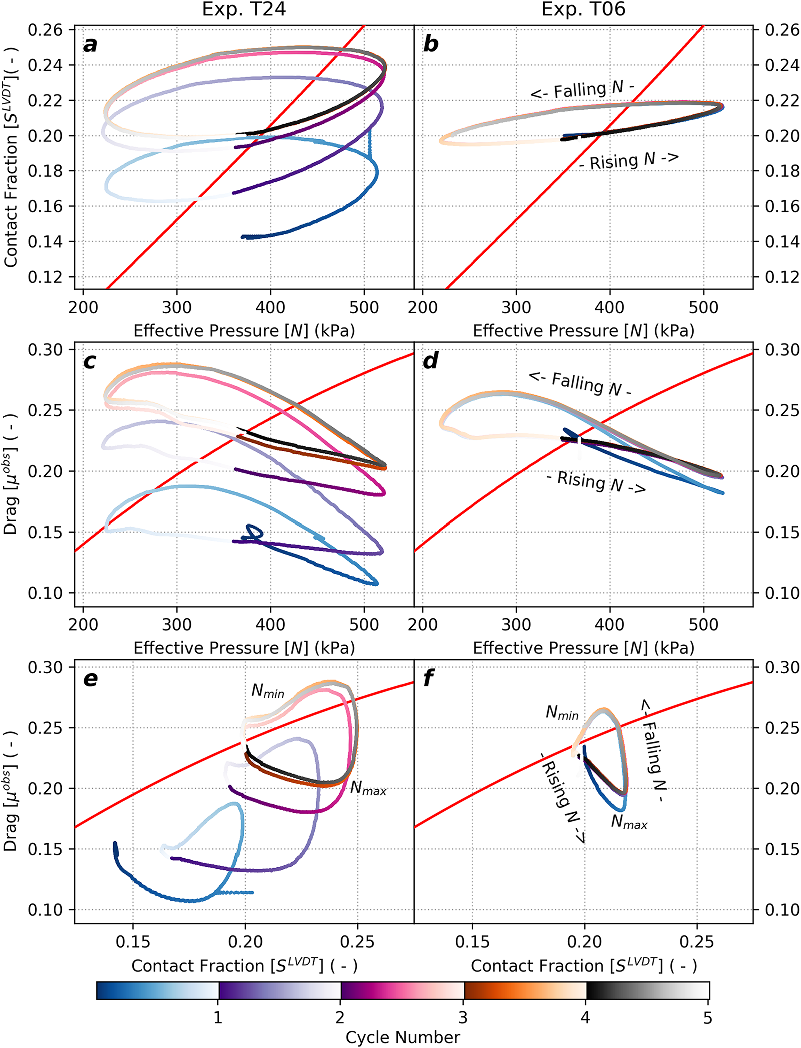
We observed the simplest hysteresis patterns between  $N$ and ${S^{LVDT}}$
(Figs 7a, b) indicating that cavity geometries oscillate with a simple phase lag relative to
${S^{LVDT}}$
(Figs 7a, b) indicating that cavity geometries oscillate with a simple phase lag relative to  $N$. In both experiments, ${\mu^{obs}}$
and
${\mu^{obs}}$
and  $N$ oscillated in anti-phase relative to expectations from analytic theory (Figs 7c, d) and exhibited a roughly linear relationship when $N$ rose, and experienced a relative, nonlinear enhancement as $N$ fell. Changes in contact area also exhibit a nonlinear relationship with drag (Figs 7e, f). During times when effective pressures are lower than average (about ${N_{min}}$; Fig. 7e) ${\mu^{obs}}$
and
${\mu^{obs}}$
and  ${S^{LVDT}}$
generally agree with analytic theory, suggesting contact size has a strong influence on drag evolution under these conditions. As
${S^{LVDT}}$
generally agree with analytic theory, suggesting contact size has a strong influence on drag evolution under these conditions. As  $N$ rose above average values drag decreased while contact areas grew, and as $N$ fell from peak values ( ${N_{max}}$
; Fig. 7e) drag rebounded with little change in contact area. These nonlinear responses are inconsistent with a strictly contact-area-modulated process framework (i.e., analytic theory) and may arise from changes in the physical properties of ice-bed contacts related to elevated effective pressures (e.g., Goldsby and Kohlstedt, Reference Goldsby and Kohlstedt2001; Skarbek and others, Reference Skarbek, McCarthy and Savage2022).
${N_{max}}$
; Fig. 7e) drag rebounded with little change in contact area. These nonlinear responses are inconsistent with a strictly contact-area-modulated process framework (i.e., analytic theory) and may arise from changes in the physical properties of ice-bed contacts related to elevated effective pressures (e.g., Goldsby and Kohlstedt, Reference Goldsby and Kohlstedt2001; Skarbek and others, Reference Skarbek, McCarthy and Savage2022).
Shear stresses and effective pressures (Figs 8a, b) cycled in a similar manner as  ${\mu^{obs}}$
and
${\mu^{obs}}$
and  $N$ (Figs 7c, d), which is to be expected because of the dependence of ${\mu^{obs}}$
on
${\mu^{obs}}$
on  $N$. This evolution of linear relationships between ${\tau^{obs}}$
and
${\tau^{obs}}$
and  $N$ when $N$ was rising and relative, nonlinear enhancement of ${\tau^{obs}}$
for comparable values of
${\tau^{obs}}$
for comparable values of  $N$ as $N$ fell similarly points to a process evolution wherein falling effective pressures enhance resisting stresses in a nonlinear manner. Unlike the ${\mu ^{obs}} - N$ relationship (Figs 7c, d), the ${\tau ^{obs}} - N$ relationship (Figs 8a, b) oscillated along the trend of model predictions. The relationships between shear stress and contact length (Figs 8c, d) also show a functional form similar to ${\mu^{obs}}$
—
${\mu^{obs}}$
— $N$ (Figs 7c, d) and ${\tau^{obs}}$
—
${\tau^{obs}}$
— $N$ (Figs 8a, b); however, the conditions under which ${{{\tau }}^{obs}}$ and ${S^{LVDT}}$
vary (non)linearly are flipped. In these cases, shear stresses provided by contact areas of the same size are enhanced nonlinearly during times when
${S^{LVDT}}$
vary (non)linearly are flipped. In these cases, shear stresses provided by contact areas of the same size are enhanced nonlinearly during times when  $N$ was rising relative to a linear relationship between ${\tau^{obs}}$
and
${\tau^{obs}}$
and  ${S^{LVDT}}$
when
${S^{LVDT}}$
when  $N$ fell (Figs 8c, d). In summary, our observations indicate the following:
1) Lags in cavity geometry changes can be explained by viscous deformation processes (Figs 7a, b).
2) The trajectory of effective pressure transients plays an appreciable role in the evolution of nonlinear enhancements of system responses within forcing cycles (Figs 7c, e and 8a, d).
3) The period of effective pressure oscillations influences the intensity of nonlinear behaviors (Figs 7c, e and 8a, d).
4) The scale of effective pressure transients relative to background conditions appears to be more important for drag evolution than in the rest of our observations (Figs 7e, f).
Cross plots for effective pressure ( $N$), shear stress ( ${{\tau }}$) and contact lengths ( $S$) during Exp. T24 (left) and Exp. T06 (right). (a–b) Shear stress as a function of effective pressure, (c–d) shear stress as a function of contact fraction. Modeled values shown in red, observed values are colored by cycle number and relative time within each cycle (color bar; see description of formatting in Figure 7).
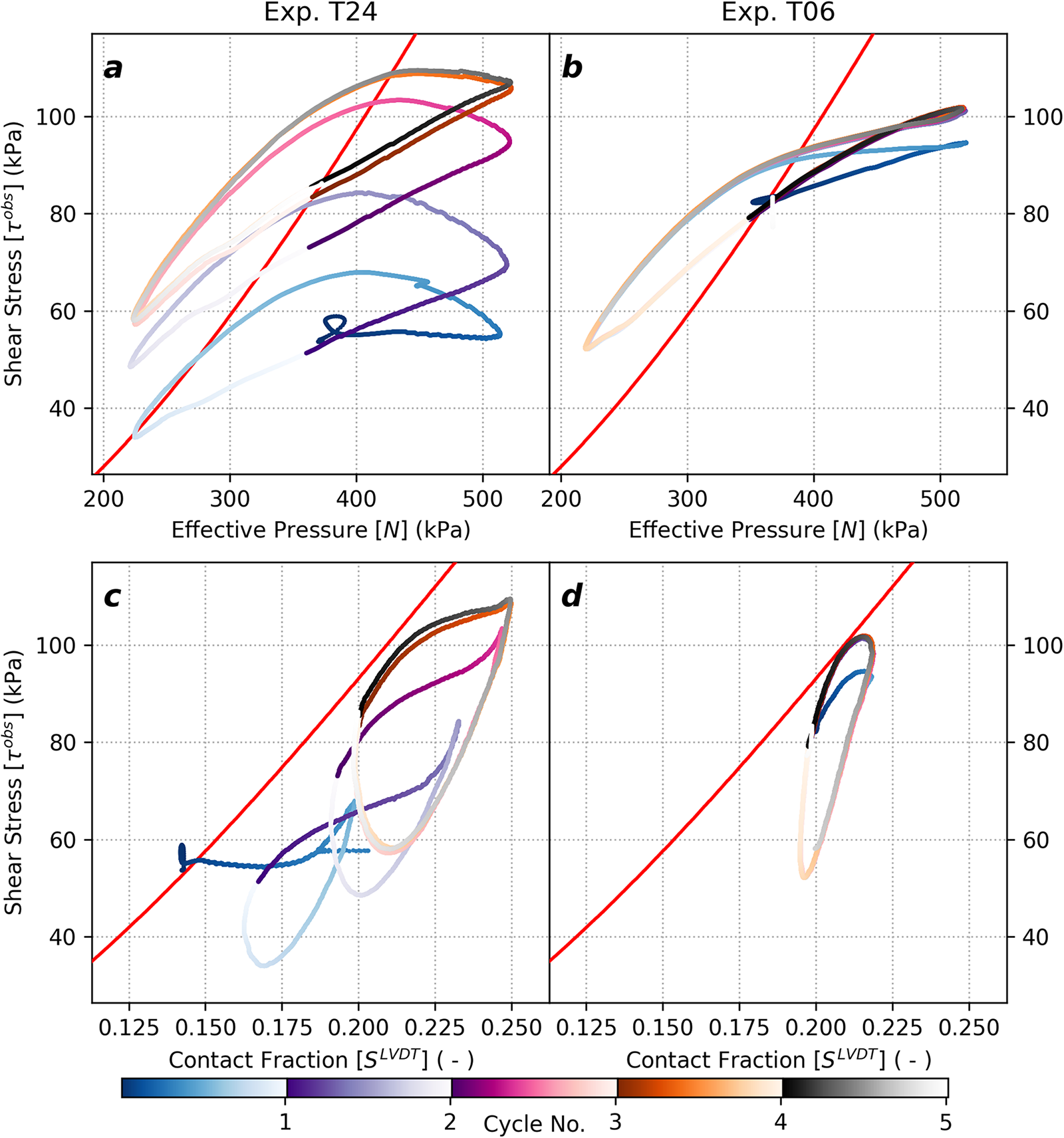
4. Discussion
4.1. Comparison to analytic theory
4.1.1 Geometric and mechanical responses
Our experimental observations significantly diverge from analytic theory on timescales of individual forcing cycles but generally conform to modeling predictions on longer timescales (Figs 4–6). Observed cavity geometries and mechanical responses oscillated in narrower ranges compared to model predictions, but all observed values fell within the range of model predictions for the range of  $N$ applied to the system (Figs 4–6). On multi-cycle timescales, observed average system responses tracked closely with model predictions (Figs 5 and 6) with some deviations observed during Exp. T24 (Figs 5c, d). We found that long-term evolution of this system’s mechanical responses could still be contributed to changes in the geometry of ice-bed contacts on the stoss side of bed obstacles (Fig. 4a), but within forcing cycles, this relationship broke down, with changes in lee contact areas correlating with transient shear stress and drag responses (Figs 4 and 5). These observations call into question the assumption that resisting forces are modulated through (stoss) contact area alone within transient forcing cycles. Additionally, the enhancement of drag and average contact area size toward the end of Exp. T24 may indicate a drag-enhancing feedback that arises from transient forcing (Figs 5c, d). Due to their late emergence in Exp. T24, it is unclear whether these enhancements are characteristic responses of the sliding system to the applied forcing, or an effect of extenuating circumstances such as the disequilibrium starting point of this experiment.
Both geometric and mechanical measurements indicate that Exp. T24 was initiated before the system reached steady-state, despite meeting the mechanical criteria used in earlier studies (Figs 4 and 5). This premature start provided a useful insight that a hard-bedded sliding system in disequilibrium can still converge to an average, near-steady-state configuration even when subjected to periodic transient forcing. Furthermore, our observations indicate that periodic transients tend to result in system responses that oscillate about a near-steady-state configuration and support the use of analytic theory to model system dynamics at time periods longer than the dominant period of relevant forcings. As such, our experiments suggest that analytic theory can still be used to model the average shear stress provided by hard beds experiencing periodic forcing for timescales longer than the dominant period of the forcing. However, modeling the average drag or cavity geometries using steady-state theory on these timescales may require adjustment.
4.1.2. Interchangeability of transient  ${U_b}$
and N forcings?
${U_b}$
and N forcings?

Our observations of characteristic lags in observed cavity geometries and drag relative to modeled values (Figs 5 and 6) match observations and modeling of comparable systems subjected to periodic  ${U_b}$
forcing (Andrews and others, 2014; de Diego and others, Reference de Diego, Farrell and Hewitt2022; Zoet and others, Reference Zoet, Iverson, Andrews and Helanow2022). This commonality suggests that periodic
${U_b}$
forcing (Andrews and others, 2014; de Diego and others, Reference de Diego, Farrell and Hewitt2022; Zoet and others, Reference Zoet, Iverson, Andrews and Helanow2022). This commonality suggests that periodic  ${U_b}$
and
${U_b}$
and  $N$ transients may be able to produce identical system responses, like steady-state theory. Fundamentally, this interchangeability arises in steady-state models because ${U_b}$
and
${U_b}$
and  $N$ modulate cavity geometries, which in turn modulate drag and resisting stresses. Our observations indicate that contact geometry alone does not fully explain observed drag and shear stress behaviors within forcing cycles (Figs 7e, f and 8c, d). As such, direct application of the physical processes underlying the steady-state equivalency of ${U_b}$
and
${U_b}$
and  $N$ forcings is not appropriate. However, ice-on-rock sliding experiments subjected to oscillatory forcing (McCarthy and others, Reference McCarthy, Skarbek and Savage2022; Skarbek and others, Reference Skarbek, McCarthy and Savage2022) may provide missing elements that support an interchangeability of periodic ${U_b}$
and
${U_b}$
and  $N$ transients for this system. Their experiments forced sliding with comparatively short period ${U_b}$
oscillations (10–100 s) and found that the oscillatory forcing shifted the system from velocity strengthening drag to velocity weakening drag. This is equivalent to the
${U_b}$
oscillations (10–100 s) and found that the oscillatory forcing shifted the system from velocity strengthening drag to velocity weakening drag. This is equivalent to the  $T$/2 lag in our drag observations and those modeled in Zoet and others (Reference Zoet, Iverson, Andrews and Helanow2022). They attribute this change to modulation of the stiffness of the ice-bed interface, which may also occur in our experiments and could provide additional support for the proposed interchangeability of transient ${U_b}$
and
${U_b}$
and  $N$ forcings for our modeled system.
Steady-state theory indicates that perturbations to  ${U_b}$
or
${U_b}$
or  $N$ can produce the same geometric and mechanical responses for cavity modulated sliding systems, and theoretical treatments of these systems often generalize the functional form of shear stress or drag with respect to ${U_b}/N$. We display our observations from both experiments for this parameterization (with ${U_b}$
= 15 m a−1) in Fig. 9. If the interchangeability of
${U_b}$
= 15 m a−1) in Fig. 9. If the interchangeability of  ${U_b}$
and
${U_b}$
and  $N$ forcings featured in steady-state theory holds true for transiently forced systems, periodic ${U_b}$
forcings might produce similar functional forms as our
${U_b}$
forcings might produce similar functional forms as our  $N$-forced observations in Fig. 9. Although drag (Fig. 9a) cycles in a manner largely inconsistent with steady-state theory, shear stresses cycle roughly parallel with model predictions (Fig. 9b) and exhibits the least amount of hysteresis of all our observations (compare to Figs 7 and 8). Data-model misfits in Fig. 9b might be reduced with modest changes in the rheologic parameters ( $B$ and $n$) selected for the steady-state model, and modulation of these parameters within cycles could further explain our observations. We explore the potential process linkages relevant to this system in the next section.
Comparison of (a) drag and (b) shear stress responses as a function of effective pressure normalized slip velocity ( ${U_b}/N$
) for steady-state model predictions (red) and observed values from exp. T24 (black) and Exp. T06 (blue) during cycles with stable mean cavity geometries (cycle numbers in key; also see Figs 3 and 5–8). All estimates shown use
${U_b}/N$
) for steady-state model predictions (red) and observed values from exp. T24 (black) and Exp. T06 (blue) during cycles with stable mean cavity geometries (cycle numbers in key; also see Figs 3 and 5–8). All estimates shown use  ${U_b}$
= 15 m a−1.
${U_b}$
= 15 m a−1.
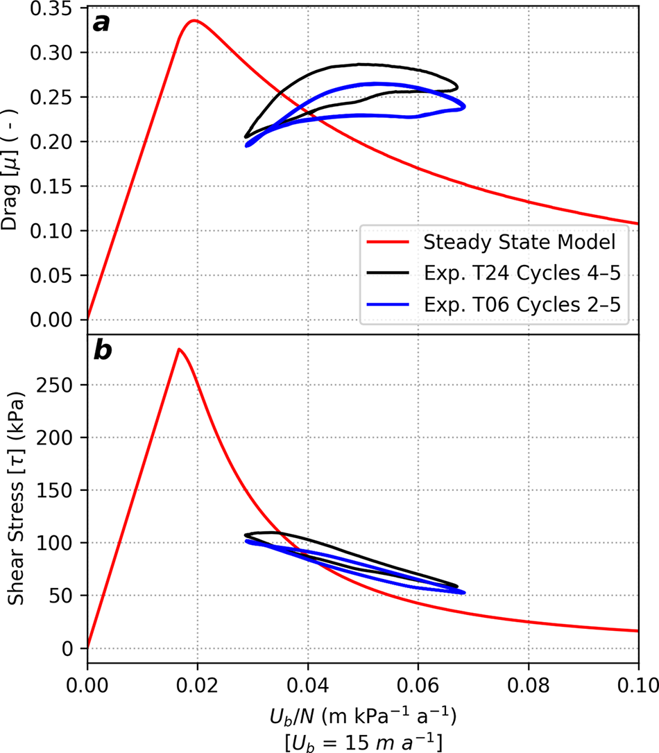
4.2. Process interpretation
We propose that the drag and resisting stress responses observed in our sliding system arise from a combination of changes in system geometry and physical properties at ice-bed contacts. The variety of hysteresis patterns observed in our experiments arose from mutual lags between system forcing, geometry and mechanical parameters that are not predicted by analytic theory (Figs 7 and 8). Common features in these patterns give insights as to the phenomena important to the evolution of drag and shear stresses in different portions of forcing cycles. The elliptic relationship between  $N$ and ${S^{LVDT}}$
(Figs 7a, b) can be explained by a simple lead-lag relationship that operates on timescales consistent with characteristic relaxation times of viscous deformation processes. This indicates that under our experimental conditions, cavity/contact-area geometry changes can be explained by viscous deformation of the ice-ring.
${S^{LVDT}}$
(Figs 7a, b) can be explained by a simple lead-lag relationship that operates on timescales consistent with characteristic relaxation times of viscous deformation processes. This indicates that under our experimental conditions, cavity/contact-area geometry changes can be explained by viscous deformation of the ice-ring.
Relationships between  $N$,
$N$,  ${\mu^{obs}}$
,
${\mu^{obs}}$
,  ${\tau^{obs}}$
and
${\tau^{obs}}$
and  ${S^{LVDT}}$
exhibit a combination of linear and nonlinear elements that trade off depending on the trajectory of effective pressures (Figs 7c, d and 8a, d). Our observations show that falling
${S^{LVDT}}$
exhibit a combination of linear and nonlinear elements that trade off depending on the trajectory of effective pressures (Figs 7c, d and 8a, d). Our observations show that falling  $N$ favors nonlinear enhancements of ${\tau^{obs}}$
and
${\tau^{obs}}$
and  ${\mu^{obs}}$
(Figs 7c, d and 8a, b) relative to comparable conditions while
${\mu^{obs}}$
(Figs 7c, d and 8a, b) relative to comparable conditions while  $N$ is rising. In contrast, we found that contact areas of comparable size corresponded to nonlinear enhancement of shear stresses when effective pressures were rising (Figs 8c, d). More complex still, ${\mu^{obs}}$
evolution relative to contact size depended more on contact size when
${\mu^{obs}}$
evolution relative to contact size depended more on contact size when  $N$ was lower than average and became highly nonlinear when $N$ was higher than average (Figs 7e, f). These behaviors demonstrate that shear stresses and drag do not evolve strictly as a function of contact geometry, as proposed by steady-state models. Instead, they appear to vary as a function of both contact geometry and stress-state-dependent processes.
Experimental measurements and numerical simulations of glacier slip commonly use the area-averaged estimate of stresses at the ice-bed interface, as calculated above, because it provides the same estimate of  $\mu $ as contact-area based estimates. Explicit calculations for ice-bed contact stresses (also referred to as local stresses, ${\sigma_{loc}}$
) demonstrate that
${\sigma_{loc}}$
) demonstrate that  ${\sigma_{loc}}$
can be much higher than
${\sigma_{loc}}$
can be much higher than  $N$ for cavity-dominated sliding systems and can influence ice flow around bed obstacles (Zoet and Iverson, Reference Zoet and Iverson2015). We calculated local stresses as ${\sigma_{loc}}$
=
${\sigma_{loc}}$
=  $N/{S^{LVDT}}$ for both experiments (Fig. 10). ${\sigma_{loc}}$
estimates range between 1.1 and 2.5 MPa in both experiments, values nearly five times larger than synchronous values of
${\sigma_{loc}}$
estimates range between 1.1 and 2.5 MPa in both experiments, values nearly five times larger than synchronous values of  $N$. This range of contact stresses straddles the transition stresses between low ( $n$ = 1.8) and high ( $n$ = 4) flow law exponents reported in Goldsby and Kohlstedt (Reference Goldsby and Kohlstedt2001; their Figure 7), with higher ${\sigma_{loc}}$
favoring
${\sigma_{loc}}$
favoring  $n$ = 4, which enhances viscous deformation rates and ‘softens’ the ice-bed interface. Skarbek and others (Reference Skarbek, McCarthy and Savage2022) attribute their experimental observations to this phenomenon and note that this effect becomes more pronounced for ice near its pressure melting point. Changes in $n$ during periods of rising $N$ may help explain the nonlinear evolution of ${\tau^{obs}}$
relative to contact area (Figs 8c, d), where initially increases with little change in
${\tau^{obs}}$
relative to contact area (Figs 8c, d), where initially increases with little change in  $S^{LVDT}$ (a ‘firm contact’ low- $n$ response) followed by diminishing enhancement of $\tau^{obs}$ with enlargement of ${S^{LVDT}}$
(a ‘soft contact’ high-
${S^{LVDT}}$
(a ‘soft contact’ high- $n$ response). Similarly, the transition to a higher- $n$ rheology relative to background conditions should diminish drag, as observed in both experiments (Figs 7c, d).
As  $N$ falls, the system should transition back to a lower- $n$ rheology, but our experiments show that this retrograde evolution is not identical to the prograde (rising $N$) evolution. Falling effective pressures lower the pressure melting point at the ice-bed interface (Eqn 2), resulting in less melt production on ice-bed interfaces. This reduced lubrication elevates drag and vice versa. This lubrication-modulation process and its effects on drag are consistent with our findings in Figs 7c, d, particularly when $N$ is higher than average. No single physical process—geometric, rheologic or thermodynamic—fully explains patterns observed in our experiments. Instead, we propose that the observed evolution of our transiently forced system arises from the interplay of these processes, with the relative importance of each process changing within transient cycles. The precise structure of this framework is under-constrained by our observations and likely requires targeted experimental work to isolate the contributions of individual processes.
Comparison of area-averaged vertical pressure ( $N$; black) and local contact pressures ( $N/{S^{LVDT}}$
; blue) for (a) Exp. T24 and (b) Exp. T06. Note the change in pressure units to mPa.
$N/{S^{LVDT}}$
; blue) for (a) Exp. T24 and (b) Exp. T06. Note the change in pressure units to mPa.
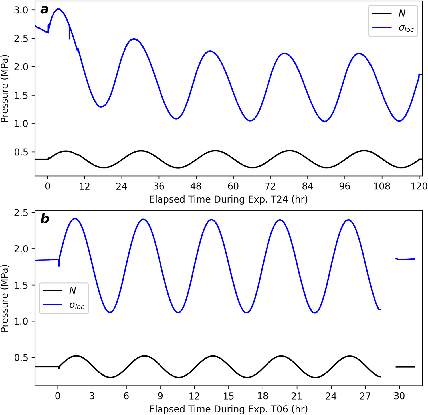
4.3. Application to field observations
Our experimental observations provide new constraints on transient, subglacial processes inferred from field observations. The 4 h lag between system forcings and cavity geometry responses observed in our experiments and in the field (Andrews and others, 2014) is used to help explain the timing and intensity of subglacial seismicity observed at hard-bedded alpine glaciers (e.g., Walter and others, Reference Walter, Deichmann and Funk2008; Stevens and others, Reference Stevens2024) and along the Greenland Ice-Sheet margin (Roeoesli and others, Reference Roeoesli, Helmstetter, Walter and Kissling2016). Stevens and others (Reference Stevens2024) observed abundant seismicity along the margins of a subglacial conduit and proposed that cavity-modulated ice-bed contacts hosted this seismicity. These cavities were subjected to large diurnal effective pressure cycles, and seismicity was most abundant in the hours after forcing peaked (following  $N_{min}$). They attribute this observation to a concentration of $\sigma_{loc}$ arising from lagged cavity dilation, consistent with our observations in Exp. T24. Our experiments show that clean ice sliding under these conditions favor increasing shear stresses (Fig. 8c) and a moderate reduction in drag (Fig. 7e), which can explain the slip deceleration observed by Stevens and others (Reference Stevens2024), but also provide unfavorable conditions for seismogenesis (e.g., Zoet and others, Reference Zoet, Carpenter and Scuderi2013; Zoet and others, Reference Zoet2020; Lipovsky and Dunham, Reference Lipovsky and Dunham2016; Lipovsky, Reference Lipovsky2019; Skarbek and others, Reference Skarbek, McCarthy and Savage2022; and references therein). Their study proposes that basal debris is a key element needed to reconcile these contrasting observations, citing experimental and theoretical studies (Zoet and others, Reference Zoet, Carpenter and Scuderi2013; Lipovsky and Dunham, Reference Lipovsky and Dunham2016; Lipovsky and others, Reference Lipovsky2019; Zoet and others, Reference Zoet2020). Our experiments provide new support for this process framework, corroborating the aspects of transient cavity geometry and resisting stresses responses to effective pressure cycles. By extension, our observations also reinforce the importance of basal debris for slip-generated seismicity and highlight the need for additional experimental constraints on transient slip behaviors with basal debris.
4.4. Glaciologic implications
Our experimental observations indicate that analytic theory remains relevant for modeling hard bedded glacier slip on timescales longer than a few days, even in the presence of oscillatory effective pressures. On timescales of individual oscillations, our experiments indicate that the geometric and mechanical responses of cavity systems are largely inconsistent with predictions from analytic theory, which could make interpreting field data collected on these short timescales difficult. Additionally, enhanced long-term-average drag observed during Exp. T24 may indicate a mechanism by which subglacial drag can be enhanced by transient forcing, but this would require additional experimentation to confirm.
Our observations corroborate recent studies that inspect cavity-modulated slip responses to oscillatory transients (de Diego and others, Reference de Diego, Farrell and Hewitt2022; McCarthy and others, Reference McCarthy, Skarbek and Savage2022; Skarbek and others, Reference Skarbek, McCarthy and Savage2022; Zoet and others, Reference Zoet, Iverson, Andrews and Helanow2022). In combination, these findings suggest that transiently forced cavities respond in a similar manner to transient oscillations of  $N$ or ${U_b}$
, which would provide a convenient extension of analytic theory for deriving a unified, transient slip rule for hard glacier beds. Similarly, our observations hint at diminishing importance of oscillatory loading effects on system responses for short period fluctuations, as illustrated by the reduced complexity in hysteresis patterns for Exp. T06 compared to Exp. T24. However, findings in Skarbek and others (Reference Skarbek, McCarthy and Savage2022) suggest that some of the phenomena that we invoke remain sensitive to oscillatory loading and important for overall slip mechanics at very short periods. We lack constraints on the effect of oscillatory loading with multi-day periods, but we hypothesize that system responses become identical to steady-state theory predictions at sufficiently long periods. Forcing periods of roughly 24 h may produce particularly strong transient behaviors in sliding systems modulated by cavities, and if this is the case, the mechanics investigated here are particularly relevant for modeling glacier systems subjected to diurnal forcing (i.e., tides and meltwater cycles), particularly on timescales comparable to—or shorter than—dominant forcing periods.
${U_b}$
, which would provide a convenient extension of analytic theory for deriving a unified, transient slip rule for hard glacier beds. Similarly, our observations hint at diminishing importance of oscillatory loading effects on system responses for short period fluctuations, as illustrated by the reduced complexity in hysteresis patterns for Exp. T06 compared to Exp. T24. However, findings in Skarbek and others (Reference Skarbek, McCarthy and Savage2022) suggest that some of the phenomena that we invoke remain sensitive to oscillatory loading and important for overall slip mechanics at very short periods. We lack constraints on the effect of oscillatory loading with multi-day periods, but we hypothesize that system responses become identical to steady-state theory predictions at sufficiently long periods. Forcing periods of roughly 24 h may produce particularly strong transient behaviors in sliding systems modulated by cavities, and if this is the case, the mechanics investigated here are particularly relevant for modeling glacier systems subjected to diurnal forcing (i.e., tides and meltwater cycles), particularly on timescales comparable to—or shorter than—dominant forcing periods.
4.5. Experimental limitations
Our experiments are not intended to replicate all the complexities of the natural world. Instead, they are intended to examine the response of a simplified system of temperate ice slipping over an idealized bed geometry when vertical pressures are systematically oscillated. Experimental limitations include the initial conditions selected (Fig. 2), the form of the forcing function (Fig. 3), the forcing parameters selected (Eqn 1) and the use of only vertical pressure modulation to drive effective pressure changes. Due to the limited number of transient sliding studies for rigid beds (i.e., de Diego and others, Reference de Diego, Farrell and Hewitt2022; Zoet and others, Reference Zoet, Iverson, Andrews and Helanow2022), there is relatively little constraint on the impacts of the initial conditions on transient system evolution. We can borrow insights from steady-state theory, but as discussed in Section 4.1, there are numerous behaviors not included in these frameworks.
Our observations show that shear stresses in both experiments converged to average values comparable to steady-state model predictions (Figs 5b and 6b), but average drag and contact sizes may experience enhancement relative to steady-state theory predictions as observed in Exp. T24 (Figs 5c, d). We lack adequate constraints on how these average cavity geometries and mechanical responses relate to initial conditions or the form of our forcing function. This makes it difficult to determine if these observations are an intrinsic features of diurnal forcings, or if they arose from some combination of experimental design choices. Similarly, we observed period-dependent behaviors that begin to illuminate a relationship between forcing oscillation periods and system responses but lack experimental constraints on forcing amplitude dependent behaviors. Numerical experiments in de Diego and others (de Diego and others, Reference de Diego, Farrell and Hewitt2022) suggest that changes in forcing amplitude produces system responses that differ from the effects of modulating the forcing period.
Our use of vertical pressure variation to modulate effective pressures contrasts some natural systems where water pressures modulate effective pressures. Although interchangeable in theory, vertical pressure modulation may produce heterogeneous stress distributions along cavity roofs and ice-bed contact areas that do not arise in water pressure modulated systems (e.g., Fig. 10). Despite these limitations, our initial transect of relevant parameter spaces provides useful insights on the response of cavity-modulated slip effective pressure transients and under what circumstances analytic theory may still be useful in modeling these systems. Further experimental work is necessary to better constrain transient system dynamics and provide a physical basis for modeling of these systems.
5. Conclusions
We conducted the first-ever experimental study of temperate glacier sliding with ice-bed separation subjected to periodic effective pressure transients using newly developed control systems at the University of Wisconsin-Madison CRSD (Fig. 1). Two experiments with 24 and 6 h oscillation periods (Fig. 3) revealed time-dependent mechanical behaviors that likely arose from a combination of geometric, rheologic and thermodynamic processes operating at ice-bed contact areas. We found that the long-term-average resisting stresses provided by our experimental system were consistent with steady-state theory (Figs 5b and 6b) and that average cavity geometries and drag generally conformed to model predictions (Figs 4, 5c, d and 6c, d). On transient timescales, the system oscillated in a variety of ways inconsistent with analytic theory. The diverse lags and cycling patterns in system responses gave rise to hysteresis not predicted by analytic theory, which also provided insights as to the processes governing transient system responses.
We directly observed cavity growth and contraction and used this to validate standard proxies for cavity geometries used in the laboratory and field (Fig. 4). Our observations indicated that cavity geometries (Figs 4, 5d and 6d) and drag (Figs 5c and 6c) systematically lagged imposed forcings. Although lags in cavity/contact geometry could be explained by viscous deformation of the ice-ring in response to effective pressure cycles, drag exhibited highly nonlinear responses requiring additional processes such as modulation of melt production or ice viscosity at ice-bed contacts. Similarly, shear stresses did not strictly vary with imposed effective pressures or ice-bed contact size (Figs 5–8), requiring consideration of these perturbed thermodynamic and rheologic properties to explain our observations in addition to the contact-geometry modulation featured in comparable steady-state theory. This framework, and our observations, are consistent with previous experimental and numerical studies that explicitly address oscillatory forcings on subglacial dynamics (de Diego and others, Reference de Diego, Farrell and Hewitt2022; McCarthy and others, Reference McCarthy, Skarbek and Savage2022; Skarbek and others, Reference Skarbek, McCarthy and Savage2022; Tsai and others, Reference Tsai, Smith, Gardner and Seroussi2022; Zoet and others, Reference Zoet, Iverson, Andrews and Helanow2022). Although our experiments provide new insights the processes governing transient slip and applicability of established and emerging sliding rules, there remains a wide swathe of parameters relevant to natural glacier systems that remain untested and warrant future numerical and experimental investigation.
Supplementary material
The supplementary material for this article can be found at https://doi.org/10.1017/jog.2025.9.
Data availability statement
Raw data and QGIS projects used to measure cavity geometries from photos are archived on MINDS@UW (https://minds.wisconsin.edu/handle/1793/89628). Additional, unprocessed time-lapse images are available upon request from the authors. Source code that reproduces all results and figures in this study are available on GitHub (https://github.com/nts345045/CRSD_CNSB.git).
Acknowledgements
This manuscript benefitted from reviews by two anonymous reviewers, A. Rempel (University of Oregon; Scientific Editor) and R. Greve (Hokkaido University; Associate Chief Editor). Formulation of our study and interpretations of our data benefitted from discussions with J. Brooks (UW-Madison), N. Morgan-Witts (UW-Madison), N. Iverson (Iowa State University), K. Feigl (UW-Madison), J. Fowler (Iowa State University), and K. Ferrier (UW-Madison). Experiment construction and operation were led by D.D. Hansen and data analyses were led by N.T. Stevens. Interpretation and drafting of this manuscript were led by N.T. Stevens and supported by D.D. Hansen and L.K. Zoet. P.E. Sobol and N.E. Lord designed, constructed, and maintain the UW-CRSD. The revision process was supported by the generosity of C.L. Bahnfleth and S.B.B. Stevens. This work was supported by NSF grants 2048315 and PR-1738913 awarded to L.K. Zoet.
Our institutions occupy traditional lands and waters of the Ho-Chunk, a place their nation has called Teejop since time immemorial, and traditional lands and waters of the Duamish, Mucleshoot, Puyallup, Suquamish and Tualip nations. We acknowledge and honor these caretakers—past and present—of these places, respect their inherent sovereignty, and strive to model their responsible stewardship.
Analyses in this work were conducted using the open-source Python libraries SciPy (Virtanen and others, Reference Virtanen2020), NumPy (Harris and others, Reference Harris2020), pandas (The Pandas Development Team, 2024) and matplotlib (Hunter, Reference Hunter2007). QGIS was used for image processing (QGIS Association, 2024). We thank these developers and contributing community members for their dedication to open-source scientific software.
Competing interests
The authors have no competing interests.
Appendix A. Steady-state Sliding Theory
The double-valued, steady-state sliding theory from Zoet and Iverson (Reference Zoet and Iverson2015) is based on Lliboutry (Reference Lliboutry1968, Reference Lliboutry1979) and Kamb (Reference Kamb1987) and models slip dynamics over a rigid, sinusoidal bed with bump elevations,  $h\left( x \right)$, calculated as
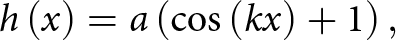 \begin{equation}h\left( x \right) = a\left( {{\rm{cos}}\left( {kx} \right) + 1} \right),\end{equation}
with amplitude,  $a$, and wavenumber $k$ (= $2\pi /\lambda $, with wavelength $\lambda $). The roof geometry of the cavity, $r\left( x \right)$ (presented as $g\left( x \right)$ in Zoet and Iverson, Reference Zoet and Iverson2015)—assuming there is no subsequent bump—is modeled as (eqn 4 in Kamb, Reference Kamb1987)
 \begin{equation}r\left( x \right) = h\left( {{1 \over 2} - {1 \over \pi }{\rm{si}}{{\rm{n}}^{ - 1}}\left( {{{2x - l} \over l}} \right) - {{2\left( {2x - 1} \right)\sqrt {x\left( {l - x} \right)} } \over {\pi {l^2}}}} \right),\end{equation}
where the length-scale of the cavity in the absence of subsequent bumps, is approximated for a nonlinear-viscous ice rheology as (eqn A2 in Zoet and Iverson, Reference Zoet and Iverson2015):
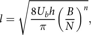 \begin{equation}l = \sqrt {{{8{U_b}h} \over \pi }{{\left( {{B \over N}} \right)}^n}} ,\end{equation}
with the sliding velocity,  ${U_b}$
, viscosity parameter,
${U_b}$
, viscosity parameter,  $B$, stress exponent, $n$ and effective pressure at the bed, $N$. We adopted values of $B$=6.3 × 10⁷ Pa s1/n and $n$=3 from Zoet and Iverson (Reference Zoet and Iverson2015) for our calculations. The effective pressure is the overburden pressure from the glacier minus subglacial water pressure, ${P_W}$
, given as
${P_W}$
, given as
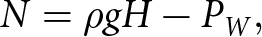 \begin{equation}N = \rho gH - {P_W},\end{equation}
with ice density  $\rho $, gravitational acceleration $g$ and ice thickness $H$. The shear stress ( $\tau$) provided by the bed with the geometry of Eqn A1 and cavity roof geometry specified by Eqns A2 and A3 is calculated as
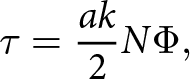 \begin{equation}\tau = {{ak} \over 2}N\Phi ,\end{equation}
Note that Eqn A5 has a ½ factor compared to the initial formulation provided in Lliboutry (Reference Lliboutry1968, Reference Lliboutry1979), which arises from later re-analysis by Lliboutry (Zoet and Iverson, Reference Zoet and Iverson2015). The bed geometry parameter in Eqn A5 is defined as
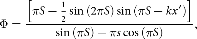 \begin{equation}\Phi = {{\left[ {\pi S - {1 \over 2}\sin \left( {2\pi S} \right)\sin \left( {\pi S - k{x^{\prime}}} \right)} \right]} \over {\sin \left( {\pi S} \right) - \pi s\cos \left( {\pi S} \right)}},\end{equation}
with ice-bed contact fraction  $S$ and critical length $x^{\prime}$, which is estimated as
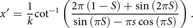 \begin{equation}{x^{\prime}} = {1 \over k}{\cot ^{ - 1}}\left( {{{2\pi \left( {1 - S} \right) + \sin \left( {2\pi S} \right)} \over {\sin \left( {\pi S} \right) - \pi s\cos \left( {\pi S} \right)}}} \right).\end{equation}
For the domain of a given cavity, the contact fraction is typically calculated as
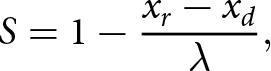 \begin{equation}S = 1 - {{{x_r} - {x_d}} \over \lambda },\end{equation}
with the cavity reattachment point  $0 \ll {x_{\rm{d}}} \lt \lambda $
and cavity detachment point
$0 \ll {x_{\rm{d}}} \lt \lambda $
and cavity detachment point  $0 \le {x_r} \ll \,\lambda $, rather than the obstacle-crest centric reference frame used in this report.
Appendix B. Parameter Summary
Summary of variable symbols, names and standard units used in this study
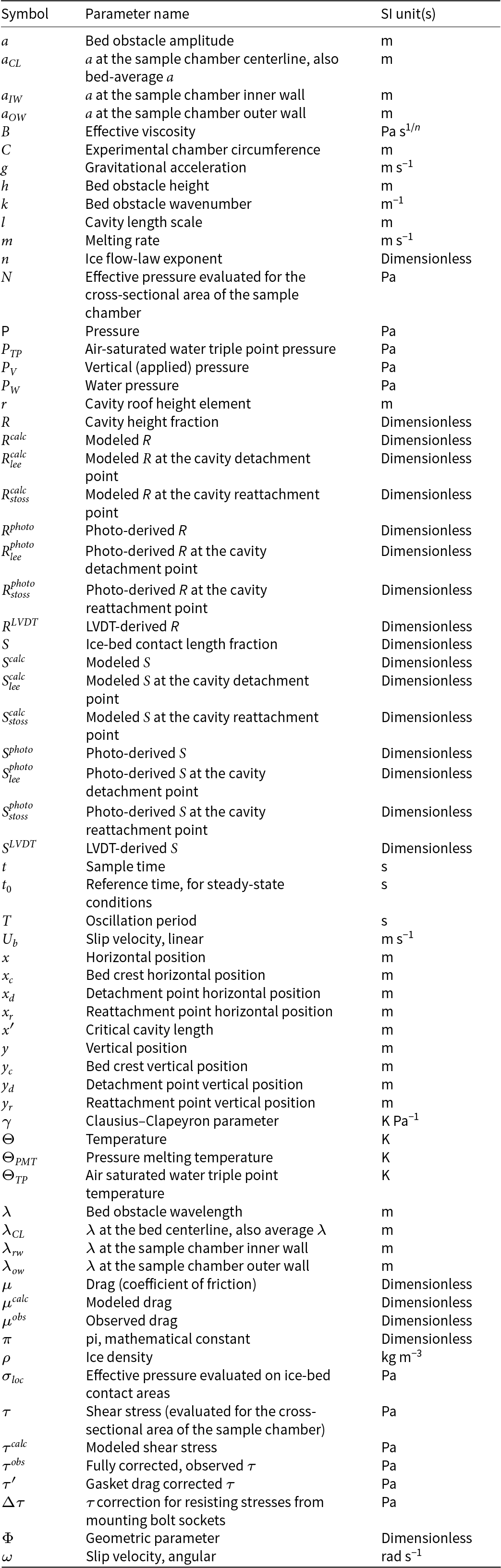


 Open access