2.1. Dynamics Model

The system error dynamic model of integrated navigation used in the Kalman filter is designed based on the INS error equations. The insignificant terms are neglected in the process of linearization (Titterton and Weston, Reference Titterton and Weston2004). The psi-angle error equations of INS are as follows (Li et al., Reference Li, Wang, Li, Gao and Tan2014):

(1) $$\delta {\dot {\bf r}} = - {{\bf \omega} _{{\rm en}}} \times \delta {\bf r} + \delta {\bf v}$$

(2) $$\delta {\dot {\bf v}} = - (2{{\bf \omega} _{{\rm ie}}} + {{\bf \omega} _{{\rm en}}}) \times \delta {\bf v} - \delta {\bf \psi} \times {\bf f} + {\bf \eta} $$

(3) $$\delta {\dot {\bf \psi}} = - ({{\bf \omega} _{{\rm ie}}} + {{\bf \omega} _{{\rm en}}}) \times \delta {\bf \psi} + {\bf \varepsilon} $$

where $\delta {\bf r}$ , $\delta {\bf v}$ and $\delta {\bf \psi} $ are the position, velocity and orientation error vectors, respectively. ${{\bf \omega} _{{\rm en}}}$ is the rate of navigation frame with respect to Earth, and ${{\bf \omega} _{{\rm ie}}}$ is the rate of Earth with respect to inertial frame. The system error dynamics of GPS/INS integration are obtained by expanding the accelerometer bias error vector ${\bf \eta} $ and the gyro drift error vector ${\bf \varepsilon} $ .

The accelerometer bias error vector ${\bf \eta} $ and the gyro drift error vector ${\bf \varepsilon} $ are regarded as the random walk process vectors, which are modelled as follows (Wang et al., Reference Wang, Lee, Hewitson and Lee2003):

(4) $${\dot {\bf \eta}} = {{\bf u}_{\rm \eta}} $$

(5) $${\dot {\bf \varepsilon}} = {{\bf u}_{\rm \varepsilon}} $$

where ${{\bf u}_{\rm \eta}} $ and ${{\bf u}_{\rm \varepsilon}} $ are white Gaussian noise vectors.

Combining Equations (1) to (5), the system dynamical model becomes:

(6) $$\left\{ {\matrix{ {\delta {\dot {\bf r}} = - {{\bf \omega} _{{\rm en}}} \times \delta {\bf r} + \delta {\bf v}} \hfill \cr {\delta {\dot {\bf v}} = - ({{\bf \omega} _{{\rm ie}}} + {{\bf \omega} _{{\rm in}}}) \times \delta {\bf v} - \delta {\bf \psi} \times {\bf f} + {\bf \eta}} \hfill \cr {\delta {\dot {\bf \psi}} = - {{\bf \omega} _{{\rm in}}} \times \delta {\bf \psi} + {\bf \varepsilon}} \hfill \cr {{\bf \eta} = {{\bf u}_{\rm \eta}}} \hfill \cr {{\bf \varepsilon} = {{\bf u}_{\rm \varepsilon}}} \hfill \cr}} \right.$$

which can be generalized in matrix and vector form:

(7) $${\dot {\bf X}} = {\bf \Phi X} + {\bf u}$$

where X is the error state vector, ${\bf \Phi} $ is the system transition matrix, and u is the process noise vector.

2.2. Observation Model

The observation model in GPS/INS integrated navigation is composed of the position and velocity difference vector between the GPS solutions and the INS computation value (Titterton and Weston, Reference Titterton and Weston2004):

(8) $$\eqalign{&{Z_{\rm r}}(t) = {r_{{\rm GPS}}}(t) - {r_{{\rm INS}}}(t) \cr & \qquad = {r_{{\rm GPS}}}(t) - \left( {{r_{{\rm INS}}}(t - \Delta t) + {v_{{\rm INS}}}(t - \Delta t) \cdot \Delta t + \displaystyle{1 \over 2}\alpha (t) \cdot \Delta {t^2}} \right)} $$

(9) $$\eqalign{&{Z_{\rm v}}(t) = {v_{{\rm GPS}}}(t) - {v_{{\rm INS}}}(t) \cr & \qquad{\hskip2pt} = {v_{{\rm GPS}}}(t) - \left( {{v_{{\rm INS}}}(t - \Delta t) + \alpha (t) \cdot \Delta t} \right)} $$

where Z _r(t) is the position error measurement vector at t time, Z _v(t) is the velocity error measurement vector, r _GPS(t) is the GPS position vector, r _INS(t) is the INS position vector, v _GPS(t) is the GPS velocity vector, v _INS(t) is the INS velocity vector, α(t) is the acceleration vector determined by the INS alone and Δt is the sample time of INS.

The generic measurement equation system of the Kalman filter can be written as:

(10) $${{\bf Z}_{\rm k}} = \left[ {\matrix{ {{Z_{\rm r}}(t)} \cr {{Z_{\rm v}}(t)} \cr}} \right] = {{\bf B}_{\rm k}}{\bf X} + \left[ {\matrix{ {{\tau _{\rm r}}} \cr {{\tau _{\rm v}}} \cr}} \right]$$

where ${{\bf B}_{\rm k}}$ is the observation matrix, and τ is the measurement noise vector, assumed to be white Gaussian noise.

4.1. Kalman Filter in GPS/INS Integrated Navigation

The Kalman filter is the most common method to realise the data fusion of different sensors. The optimal estimates of the state vector from the Kalman filter can be reached through a time update and a measurement update at a time instant:

(17) $${{\hat {\bf X}}_{\rm k}} = {{\hat {\bf X}}_{{\rm k},{\rm k} - 1}} + {{\bf G}_{\rm k}}({{\bf Z}_{\rm k}} - {{\bf B}_{\rm k}}{{\hat {\bf X}}_{{\rm k},{\rm k} - 1}})$$

(18) $${{\bf G}_{\rm k}} = {{\bf P}_{{\rm k},{\rm k} - 1}}{\bf B}_{\rm k}^{\rm T} {({{\bf B}_{\rm k}}{{\bf P}_{{\rm k},{\rm k} - 1}}{\bf B}_{\rm k}^{\rm T} + {{\bf R}_{\rm k}})^{ - 1}}$$

(19) $${{\hat {\bf X}}_{{\rm k},{\rm k} - 1}} = {{\bf \Phi} _{{\rm k},{\rm k} - 1}}{{\hat {\bf X}}_{{\rm k} - 1}}$$

(20) $${{\bf P}_{{\rm k},{\rm k} - 1}} = {{\bf \Phi} _{\rm k}}{{\bf P}_{{\rm k} - 1}}{\bf \Phi} _{\rm k}^{\rm T} + {{\bf Q}_{\rm k}}$$

(21) $${{\bf P}_{\rm k}} = ({\bf I} - {{\bf G}_{\rm k}}{{\bf B}_{\rm k}}){{\bf P}_{{\rm k},{\rm k} - 1}}$$

where ${{\bf G}_{\rm k}}$ is the gain matrix of Kalman filter at time k, ${{\bf P}_{\rm k}}$ is the covariance matrix of state vector at time k, ${{\bf R}_{\rm k}}$ is the covariance matrix of measurement noise vector at time k, ${{\bf Q}_{\rm k}}$ is the covariance matrix of process noise at time k, and the subscript k,k-1 represents the state and covariance estimates forward from time k-1 to time k.

In a closed loop integration scheme, a feedback loop is used for correcting the systematic errors. In this way, the mechanisation performs a simple navigation calculation under the assumption of small errors. In this case, the error states will be reset to zero after every measurement update (Godha, Reference Godha2006). Thus, the navigation resolution is expressed by:

(22) $${{\hat {\bf X}}_{\rm k}} = {{\bf P}_{{\rm k},{\rm k} - 1}}{\bf B}_{\rm k}^{\rm T} {({{\bf B}_{\rm k}}{{\bf P}_{{\rm k},{\rm k} - 1}}{\bf B}_{\rm k}^{\rm T} + {{\bf R}_{\rm k}})^{ - 1}}{{\bf Z}_{\rm k}}$$

4.2. Uncertainty of GPS Observation Expansion

GPS observation expansion is able to increase the filter frequency, while it brings the data uncertainty to the GPS/INS integrated navigation. To control the uncertainty of GPS observation expansion, it should be described quantitatively. Although it is feasible to apply the GPS position information (x _T , y _T) to filter and update the states at time T + 0·01 s, T + 0·02 s, the PDF at the time T + 0·01 s, T + 0·02 s … is decreasing with respect to the PDF at time T. This indicates that the uncertainty of the expanded GPS observation of T + 0·01 s, T + 0·02 s, … increases. The uncertainty growth of the GPS positions will decrease the filter accuracy. In order to know the depth of uncertainty well, the information entropy can be used to describe the uncertainty of the expanded GPS observation.

The information entropy is used to measure how much information is in an event. The larger uncertainty a variable has, the more complex information it will contain, or it will have a larger information entropy. The information entropy can be defined as (Xu et al., Reference Xu, Ma and Su2011):

(23) $$H = - \int\!\!\!\int_R {\,f\,(x,y) \cdot \ln \vert f\,(x,y) \vert dxdy} $$

From Equations (13) and (23), the information entropy of GPS position observation is

(24) $$H = \left( {\ln \displaystyle{1 \over {2\pi {\sigma ^2}}} - \displaystyle{{{r^2}} \over {2{\sigma ^2}}} - 1} \right) \cdot {e^{\textstyle{{{r^2}} \over {2{\sigma ^2}}}}} - \ln \displaystyle{1 \over {2\pi {\sigma ^2}}} + 1$$

where $r = \sqrt {{{\left( {x - {x_{\rm T}}} \right)}^2} + {{\left( {y - {y_{\rm T}}} \right)}^2}} $ is the distance between the current position (x, y) and its mathematical expectation (x _T , y _T).

The derivative of Equation (24) is given by

(25) $$H^{\prime} = - \displaystyle{r \over {{\sigma ^2}}} \cdot {e^{\textstyle{{{r^2}} \over {2{\sigma ^2}}}}}\left( {\ln \displaystyle{1 \over {2{\rm \pi} {\sigma ^2}}} - \displaystyle{{{r^2}} \over {2{\sigma ^2}}}} \right)$$

if σ is larger than $1/\sqrt {2{\rm \pi}} $ , and the derivative H′ is bigger than zero. In GPS/INS integrated navigation, the σ of GPS position from single point positioning is larger than one metre, which implies that the information entropy of expanded GPS observation is the increasing function of the variable r. During the GPS observation expansion, the further the expansion of the observation is with respect to the mathematical expectation, the larger uncertainty it will have.

4.3. Adaptive Filter with GPS Observation Expansion

In order to control the influence of growing uncertainty in GPS observation expansion, the adaptive filter can be deployed. The common adaptive filter resolution is generally expressed as:

(26) $${{\hat {\bf X}}_{\rm k}} = {{\hat {\bf X}}_{{\rm k},{\rm k} - 1}} + {{\bar {\bf G}}_{\rm k}}({{\bf Z}_{\rm k}} - {{\bf B}_{\rm k}}{{\hat {\bf X}}_{{\rm k},{\rm k} - 1}})$$

where ${{\bar {\bf G}}_{\rm k}}$ is the adaptive Kalman filter gain matrix (Yang and Gao, Reference Yang and Gao2006):

(27) $${{\bar {\bf G}}_{\rm k}} = \displaystyle{1 \over {{\alpha _{\rm k}}}}{{\bf P}_{{\rm k},{\rm k} - 1}}{\bf B}_{\rm k}^{\rm T} {(\displaystyle{1 \over {{\alpha _{\rm k}}}}{{\bf B}_{\rm k}}{{\bf P}_{{\rm k},{\rm k} - 1}}{\bf B}_{\rm k}^{\rm T} + {{\bf R}_{\rm k}})^{ - 1}}$$

with a feedback loop, the adaptive filter resolution can be simplified to:

(28) $${{\hat {\bf X}}_{\rm k}} = \displaystyle{1 \over {{\alpha _{\rm k}}}}{{\bf P}_{{\rm k},{\rm k} - 1}}{\bf B}_{\rm k}^{\rm T} {(\displaystyle{1 \over {{\alpha _{\rm k}}}}{{\bf B}_{\rm k}}{{\bf P}_{{\rm k},{\rm k} - 1}}{\bf B}_{\rm k}^{\rm T} + {{\bf R}_{\rm k}})^{ - 1}}{{\bf Z}_{\rm k}}$$

in which α _k is the adaptive factor.

During GPS observation expansion, the expansion information due to the uncertainty will bring outlier disturbance. Thus, $\alpha _{\rm k}^{\rm H} $ is introduced to decrease or even eliminate the outlier disturbance. On the basis of the uncertainty of the expanded GPS position observations, $\alpha _{\rm k}^{\rm H} $ is defined by:

(29) $$\alpha _{\rm k}^{\rm H} = 1 - H$$

where H is the uncertainty in current time.

Except where the adaptive factor can decrease or eliminate the abruptness of GPS observation expansion, it can also be used to inhibit the influence of gross errors on the GPS observation. Accordingly, the adaptive factor $\alpha _{\rm k}^{\rm e} $ is introduced based on predicted residual (Mohamed and Schwarz, Reference Mohamed and Schwarz1999):

(30) $$\alpha _{\rm k}^{\rm e} = \left\{ {\matrix{ 1 & { \vert \Delta {V_{\rm k}} \vert \le {\rm c}} \cr {\displaystyle{{\rm c} \over {{\rm \vert} \Delta {V_{\rm k}}{\rm \vert}}}} & { \vert \Delta {V_{\rm k}} \vert \gt {\rm c}} \cr}} \right.$$

where c is a constant between 0·85 and 1·0.

The learning statistic ΔV _k is constructed as follows

(31) $$\Delta {V_{\rm k}} = \displaystyle{{{\bf V}_{\rm k}^{\rm T} {{\bf V}_{\rm k}}} \over {{\rm tr}({{\bf B}_{\rm k}}{{\bf P}_{{\rm k},{\rm k} - 1}}{\bf B}_{\rm k}^{\rm T} + {{\bf R}_{\rm k}})}}$$

(32) $${{\bf V}_{\rm k}} = {{\bf Z}_{\rm k}} - {{\bf B}_{\rm k}}{{\hat {\bf X}}_{{\rm k},{\rm k} - 1}}$$

The following should be noted about the proposed filter method. Firstly, when the GPS observation contaminated by gross error at the time of T is used to implement the filter update as GPS observation expansion, the Kalman filter solution suffers from gross error and outlier disturbance due to observation expansion, which can easily lead to a filter divergence. Hence, the GPS observation expansion should not be performed at the time T + 0·01 s, T + 0·02 s …in the case that GPS observation is affected by gross error at the time of T. Secondly, because the vertical accuracy of a GPS position is much lower than the horizontal accuracy, GPS observation expansion only makes use of horizontal position. Thirdly, if the position at the current time is far away from the position at the time of T, the expanding observation with large uncertainty is used to perform the measurement update of the states, which may easily lead to a major outlier. In that case, the GPS observation expansion may be counter-productive. Therefore, the GPS measurement expansion with large uncertainty should be rejected by setting up a threshold β.

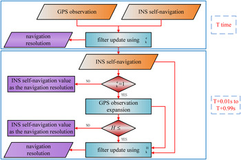
We schematically present a block diagram in Figure 2 to outline the fundamental mechanism of the proposed adaptive filter method. The flow of the proposed adaptive filter with GPS observation expansion can be summarised as follows:

1. 1) At the time T, resolve the navigation result by the adaptive filter with the GPS observation (x _T , y _T) using the adaptive factor $\alpha _{\rm k}^{\rm e} $ ( ${\alpha _{\rm k}} = \alpha _{\rm k}^{\rm e} $ );

2. 2) For the further time instants from T + 0·01 s to T + 0·99 s, if $\alpha _{\rm k}^{\rm e} \lt 1$ at time T, the navigation results only make use of the free inertial navigation solution without observation expansion;

3. 3) If $\alpha _{\rm k}^{\rm e} = 1$ at the time T, calculate the distance r between the current position with (x _T , y _T) and obtain the uncertainty H using Equation (16);

4. 4) If H ≤ β, calculate the adaptive factor $\alpha _{\rm k}^{\rm H} $ and perform the adaptive filter update using the expanded GPS observation ( ${\alpha _{\rm k}} = \alpha _{\rm k}^{\rm H} $ ). Otherwise, only the inertial self-navigation is introduced;

5. 5) If H > β, the integrated navigation does not perform any measurement update using GPS observation expansion, until the GPS receiver delivers the new position information, and then repeats the steps above.

Figure 2. The proposed adaptive filter with GPS observation expansion

According to the above description, the adaptive factor $\alpha _{\rm k}^{\rm e} $ is only used at the time when the GPS observation inputs and the adaptive factor $\alpha _{\rm k}^{\rm H} $ is only applied during GPS observation expansion. The two kinds of factor are not used at the same time to avoid filter divergence. If one compares the adaptive filter using GPS observation expansion with the standard Kalman filtering, one can find the following: (1) GPS observation expansion increases the frequency of the observation updates for the time between two GPS observation epochs; (2) the adaptive filter with GPS observation expansion can not only control the effect of GPS measurement errors on the states, but also lessens the influence of outliers due to GPS observation expansion; (3) the proposed GPS observation expansion is based on the dynamic characteristics of a vehicle itself, which relies on the velocity of the vehicle. The Kalman filter will be processed more times in the proposed method and the corresponding amount of calculation will be increased. Not too many conditions meet the requirements of GPS observation expansion, so the overall calculation burden will not be significantly increased. On the other hand, the key of navigation work is real-time performance. So the different operations in GPS/INS integrated navigation have been set on different priorities. The GPS observation expansion algorithm is one assisting method and its priority is the lowest to make sure that it will not impact the real-time performance.

5.1. Test One

To test the efficiency of the proposed method, a land vehicle field test was carried out. The field test was conducted in the Daxing district of Beijing. An overview of the test trajectory is given in Figure 3. The road condition is complex and diverse including city circular road, street area and bridge overpass. The whole test lasts about half an hour. The MEMS IMU ran at the data rate of 100 Hz and its technical data is shown in Table 2. The GPS receiver was used at the data rate of 1 Hz. A SPAN-CPT (Synchronous Position, Attitude and Navigation combined GNSS and INS) product by NovAtel Inc., together with the MEMS-IMU was installed in the vehicle. One GPS antenna was installed on the roof of the vehicle and another GPS receiver was set on a known point as the dynamical differential GPS reference station. The post-processed differential GPS solutions were used as the position reference value and the post-processed SPAN-CPT outputs were used as the velocity and attitude reference value and their accuracies are shown in Table 3.

Figure 3. The trajectory of test one.

Table 2. The MEMS-IMU's technical data.

Table 3. The reference value accuracy.

In the data processing, the initial parameters of the Kalman filter for the integrated navigation were determined based on experience. The initial position errors were 3 m, 3 m and 5 m and the initial velocity errors were 0·1 m/s, 0·1 m/s and 0·5 m/s in NED (North-East-Down) directions, respectively. The initial platform alignment errors were 0·01°, 0·01°, 0·1°. The initial standard deviations of gyro and accelerometer biases were 10°/h and 500 mg, respectively. The initial standard deviation of GPS position and velocity were 3·3 m and 0·1 m/s. The alignment information can be obtained with INS and GPS information in static condition. The initial position, velocity and attitude are set the same for different schemes to obtain a better comparison performance.

In order to test the efficiency of the new method, three calculation schemes are performed:

• Scheme 1: the standard Kalman filter,

• Scheme 2: the adaptive Kalman filter without GPS observation expansion (Yang and Gao, Reference Yang and Gao2006),

• Scheme 3: the enhanced GPS/INS integrated navigation system with GPS observation expansion (the proposed method in this paper).

The whole analysis focuses on four road conditions: 1. High-speed (velocity ⩾ 40 km/h) and straight road, 2. High-speed and curving road, 3. Low-speed (velocity < 40 km/h) and straight road, 4. Low-speed and curving road.

Figure 4 shows the trajectory chart of the reference and three schemes. One local area of the four road conditions mentioned above was chosen and shown in Figure 5. In order to compare the error in different regions of Figure 5, the horizontal position error series of three schemes is shown in Figure 6. Whether on straight roads or on curving roads, the navigation solution of three schemes in high speed conditions was almost the same. However, the navigation result from Scheme 3 was better than the result from Scheme 1 and Scheme 2 when the vehicle was driven at low speed. This was due to the fact that the vehicle in high-speed conditions was leaving from the position at the time T in a short time span. The expanding GPS observations were very few or even non-existent, which would weaken the effect of the GPS observation expansion.

Figure 4. Trajectory comparison of different schemes.

Figure 5. Trajectory comparison of different motion regions (enlargement): (a) High-speed straights region; (b) High-speed corners region; (c) Low-speed straights region; (d) Low-speed corners region.

Figure 6. Horizontal position error comparison of different motion regions: (a) High-speed straights region; (b) High-speed corners region; (c) Low-speed straights region; (d) Low-speed corners region.

Figure 7 shows the time series of position error from three schemes vs. dynamical differential GPS solution in the NED directions. A statistical summary of the Root Mean Square errors (RMS) and maximum value for position error is presented in Table 4. From the whole trajectory, the navigation accuracy with Scheme 2 was little better than the accuracy with Scheme 1. The navigation accuracy for Scheme 3 was superior to the accuracy from Scheme 1 and Scheme 2. The adaptive filter (Scheme 2) could resist the impact of dynamics model outliers on the state estimates. The GPS observation expansion (Scheme 3) could not only increase the measurement update rate, but also inhibit the negative effect of the growing uncertainty from the expanding GPS observation, which can improve the navigation accuracy and prevent the filter from diverging. The results show that the position of Scheme 3 can achieve an accuracy of 0·852 m, 0·946 m and 0·951 m in the north, east and down coordinate components, respectively. Compared with Scheme 1, the position accuracy in the north, east and down directions is improved by 69%, 67% and 16% for Scheme 3 respectively. Compared with Scheme 2, the position accuracy in the north, east and down directions are improved by 43%, 43% and 11% for Scheme 3 respectively. Because only the horizontal coordinate is brought in the GPS observation expansion, δr _N and δr _E are the directly measurable variables and δr _D is the indirectly measurable variable. So the accuracy improvement in the north and east directions is larger than that in the down direction.

Figure 7. The position error for different schemes: (a) position error in north; (b) position error in east; (c) position error in down.

Table 4. Comparison of three schemes in terms of position error.

Table 5 shows the velocity improvement realized by the enhanced GPS/INS integrated navigation system with GPS observation expansion proposed in the paper. Figure 8 plots the integrated system velocity errors in north, east and down directions respectively. The results show that the velocity of Scheme 3 can achieve an accuracy of 0·304 m/s, 0·304 m/s and 0·118 m/s in the north, east and down coordinate components, respectively, which is a better performance than Scheme 1 and Scheme 2. Compared to Scheme 1, the proposed enhanced GPS/INS integrated navigation system improves all the velocity errors in the north, east and down direction by 45%, 47% and 1% RMS, respectively. The velocity accuracies of three schemes are almost of the same level in the down direction. Because the velocity is very small in the north direction for land vehicles, the velocity value is set to zero at the beginning of the INS self-navigation computation period, which is one non-holonomic constraint for land vehicles.

Figure 8. The velocity error for different schemes: (a) velocity error in north; (b) velocity error in east; (c) velocity error in down.

Table 5. Comparison of three schemes in terms of velocity error.

The roll, pitch and yaw errors of Scheme 1, Scheme 2 and Scheme 3 are given in Figure 9 and Table 6. It can be seen that the attitude accuracy has been improved with Scheme 3. In terms of RMS, compared with Scheme 1 (3·763°) and Scheme 2 (3·254°), the error from Scheme 3 dropped down to 2·709°in yaw attitude. The largest attitude errors of roll, pitch and yaw angles are 0·399°, 0·261° and 6·005°, respectively, when Scheme 1 is used. By contrast, the largest attitude errors are 0·304°, 0·194° and 4·701° when the proposed approach is applied, which are considerably smaller.

Figure 9. The attitude error for different schemes: (a) attitude error in roll; (b) attitude error in pitch; (c) attitude error in yaw.

Table 6. Comparison of three schemes in terms of attitude error.

5.2. Test Two

Longer field tests were conducted to evaluate the performance of the proposed method. The test systems are the same as test one. The field test was conducted in China University of Mining and Technology of Xuzhou. An overview of the test trajectory is given in Figure 10.The whole time of the test was about two hours. The three calculation schemes of test one were performed.

Figure 10. The trajectory of test two.

Shown in Figure 11 are time series of position solution differences with respect to the reference value from different schemes. Table 7 illustrates RMS and maximum values of position error. The results of test two are similar to those of test one. The results show that the position of Scheme 3 can achieve an accuracy of 0·845 m, 0·768 m and 2·399 m in the north, east and down coordinate components, respectively. Compared with Scheme 1, the position accuracy in the north, east and down directions are improved by 62%, 56% and 51% for Scheme 3 respectively. The result shows that the enhanced GPS/INS integrated navigation system with GPS observation expansion is able to realise better performance in longer term navigation work.

Figure 11. The position error for different schemes: (a) position error in north; (b) position error in east; (c) position error in down.

Table 7. Comparison of three schemes in terms of position error.