

Introduction
Projecting how much the Greenland ice sheet will contribute to sea-level rise continues to be a challenge for numerous reasons, including low model resolution, unknown boundary conditions, model physics which remain incapable of simulating ice-stream acceleration, and the current inability to couple climate and ice-sheet models to include adequate feedback between surface mass-balance and elevation changes (e.g. Reference SolomonSolomon and others, 2007; Reference Vaughan and ArthernVaughan and Arthern, 2007; Reference JoughinAlley and Joughin, 2012). Mostly satellite-based, the recent observations of mass (Reference ShepherdShepherd and others, 2012; Reference Luthcke, Sabaka, Loomis, Arendt, McCarthy and CampLuthcke and others, 2013), surface velocities (Reference JoughinJoughin and others, 2012; Reference Moon, Joughin, Smith and HowatMoon and others, 2012), surface elevations (Reference SørensenSørensen and others, 2011) and ice discharge (Reference Rignot and KanagaratnamRignot and Kanagaratnam, 2006; Reference Howat, Joughin and ScambosHowat and others, 2007) portray a rapidly evolving ice sheet in greater detail (e.g. Reference Rignot and KanagaratnamRignot and others, 2011) and highlight the complex and regionally variable interplay between ice discharge, precipitation, surface melting and runoff (Reference SasgenSasgen and others, 2012). The area that has experienced melt has been gradually increasing (Reference TedescoTedesco and others, 2013), amplified by an albedo feedback that may enlarge the area to a significant portion of the ice sheet within a few decades (Reference Box, Fettweis, Stroeve, Tedesco, Hall and SteffenBox and others, 2012). Concomitantly, total mass losses are increasing. The dynamics along the margins of the ice sheet are also changing, so that tidewater outlet glaciers have not only been seen to accelerate, thin and retreat, but even subsequently to decelerate and readvance (e.g. Reference Luckman, Murray, de Lange and HannaLuckman and others, 2006; Reference Rignot and KanagaratnamRignot and Kanagaratnam, 2006; Reference Velicogna and WahrVelicogna and Wahr, 2006; Reference Howat, Joughin and ScambosHowat and others, 2007; Reference Wouters, Chambers and SchramaWouters and others, 2008; Reference Pritchard, Arthern, Vaughan and EdwardsPritchard and others, 2009; Reference Rignot and KanagaratnamRignot and others, 2011; Reference SørensenSørensen and others, 2011; Reference Moon, Joughin, Smith and HowatMoon and others, 2012; Reference KhanKhan and others, 2013).
Large-scale modeling efforts for both the Greenland and Antarctic ice sheets have been somewhat hindered by low resolutions as well as by undetermined boundaries and initial conditions, and the models remain incapable of describing high-velocity ice streams realistically (e.g. Reference Ridley, Huybrechts, Gregory and LoweRidley and others, 2005; Reference Gregory and HuybrechtsGregory and Huybrechts, 2006; Reference Vizcaíno, Mikolajewicz, Jungclaus and SchurgersVizcaíno and others, 2010). For these reasons, model studies to date have been unable to assess whether the developments observed represent minor perturbations prior to stabilization, or rather a major trend that may affect sea level (Reference Alley, Clark, Huybrechts and JoughinAlley and others, 2005). By applying an advanced model to the Greenland ice sheet, a recent study showed that ice discharges can adjust rapidly to dynamic perturbation, thereby establishing that local surface mass balance will need two-way coupling with ice-sheet models to ensure their predictive ability (GilletChaulet and others, 2012). On centennial timescales, attempts to couple climate with large-scale ice-sheet models indicate that while ice-sheet responses hardly affect global climate, they can significantly impact local and regional temperatures, atmospheric circulation and precipitation (Reference Ridley, Huybrechts, Gregory and LoweRidley and others, 2005; Reference Mikolajewicz, Vizcaíno, Jungclaus and SchurgersMikolajewicz and others, 2007). New models have been emerging to address the above limitations. For instance, surface mass-balance models with a high resolution show not only more mass-balance turnover (Reference EttemaEttema and others, 2009) and runoff (Reference HannaHanna and others, 2008; Reference Mernild, Liston, Hiemstra and ChristensenMernild and others, 2010), but also the significance of ocean/ice interactions (Reference Holland, Thomas, Young, Ribergaard and LyberthHolland and others, 2008; Reference Docquier, Perichon and PattynDocquier and others, 2011; Reference Vieli and NickVieli and Nick, 2011). Finally, a number of studies have highlighted the requirement for finer model resolutions of precipitation patterns and topographical features in order to advance the scientific understanding of climatic mass balance regarding the Greenland ice sheet (Reference Box, Bromwich and BaiBox and others, 2004, Reference Box2006; Reference Fettweis, Gallée, Lefebre and Van YperseleFettweis and others, 2005; Reference EttemaEttema and others, 2009; Reference Lucas-Picher, Wulff-Nielsen, Christensen, Aðalsgeirsdóttir, Mottram and SimonsenLucas-Picher and others, 2012).
On both decadal and centennial timescales, projections of ice-sheet responses resemble the use of weather-forecasting models, because the initial model state strongly affects model responses (Reference Arthern and GudmundssonArthern and Gudmundsson, 2010; Reference Aschwanden, Aðalsgeirsdóttir and KhroulevAschwanden and others, 2013). Therefore, capturing the observed present-day trends in ice mass is crucial for projecting future developments reliably. Hindcasting has been suggested for validating the initial states of models and thereby increasing confidence in model responses (Reference Aschwanden, Aðalsgeirsdóttir and KhroulevAschwanden and others, 2013). Large-scale ice-sheet models are currently being developed that should be capable of simulating observed mass losses (Reference Ren, Fu, Leslie, Karoly, Chen and WilsonRen and others, 2011; Reference Gillet-ChauletGillet-Chaulet and others, 2012; Reference Larour, Seroussi, Morlighem and RignotLarour and others, 2012; Reference Brinkerhoff and JohnsonBrinkerhoff and Johnson, 2013).
A number of methods have been suggested for initializing an ice-sheet model. One common procedure is to run the model through a full glacial cycle (125 ka), applying climate records from ice cores to parameterize the fluctuations in climate forcing (e.g. Reference Letréguilly, Reeh and HuybrechtsLetréguilly and others, 1991; Reference Ritz, Fabre and LetréguillyRitz and others, 1996; Reference HuybrechtsHuybrechts, 2002; Reference GreveGreve, 2005). However, this often results in an ice sheet that differs in size and shape from the observed present-day sheet, thereby introducing potential biases in ice dynamics. Inverse methods, while faithful to observed ice-sheet geometry, may nonetheless lead to some inconsistencies with the forcing fields and eventually to model drift. One solution has been to combine more than one method while creating the initial state, which calls for obtaining temperature fields from glacial cycle runs, in addition to making the model conform with observed ice-sheet geometry and velocity (Reference GoelzerGoelzer and others, 2013). An example of this approach would be to locally adjust the basal drag coefficient and then to run model simulations that would permit surface evolution in response to forcing, thereby relieving the initial state from constraints imposed by the initialization procedure (e.g. Reference Gillet-ChauletGillet-Chaulet and others, 2012; Reference Seddik, Greve, Zwinger, Chaulet and GagliardiniSeddik and others, 2012).
This paper presents the results of simulations performed with the Parallel Ice Sheet Model (PISM; Reference Khroulev and PISMKhroulev and PISM Team, 2012). The study is designed to assess the sensitivity of sea-level rise projections to (1) climate-forcing fields, (2) the method of initializing the ice-sheet model, and (3) the average present-day climate that is assumed for the initial state, and added to anomalies in the scenario runs. Four initializing methods are applied, three of which are similar to those used by Reference Aschwanden, Aðalsgeirsdóttir and KhroulevAschwanden and others (2013). The various initial states are subsequently forced with the output from three dynamic regional climate models (RCMs), which are used to downscale the climate output fields of two general circulation models (GCMs, i.e. ECHAM5 and HadCM3) according to two emissions scenarios (A1B and E1). The climate model fields are adopted from the European Union’s Seventh Framework Programme (EU FP7) project ice2sea. The resulting sea-level contributions are presented in terms of 21st-century cumulative mass losses from the Greenland ice sheet.
Methods
The Parallel Ice Sheet Model (PISM)
PISM (http://www.pism-docs.org) is an open-source, parallel, high-resolution ice-sheet model (Reference Bueler, Lingle and BrownBueler and others, 2007; Reference Bueler and BrownBueler and Brown, 2009; Aschwanden and others, 2012) that has been applied in numerous studies of the Greenland and Antarctic ice sheets (Reference MartinMartin and others, 2011; Reference Solgaard, Reeh, Japsen and NielsenSolgaard and others, 2011; Reference WinkelmannWinkelmann and others, 2011; Reference Solgaard and LangenSolgaard and Langen, 2012; Reference Aschwanden, Aðalsgeirsdóttir and KhroulevAschwanden and others, 2013). The simulations described here use similar model version, set-up and forcing methods to those used by Reference Aschwanden, Aðalsgeirsdóttir and KhroulevAschwanden and others (2013) for hindcasting (development revisions based on stable version 0.4). As a hybrid stress balance model, PISM solves both shallow-shelf and shallow-ice approximations (SSA and SIA, respectively) of the stress balance equations from which it combines the solutions (Reference Bueler and BrownBueler and Brown, 2009). The thermodynamic equation is solved in terms of enthalpy rather than temperature, enabling solutions for polythermal ice masses (Reference Aschwanden, Bueler, Khroulev and BlatterAschwanden and others, 2012). For basal sliding, a nearly-plastic power law (Reference Schoof and HindmarshSchoof and Hindmarsh, 2010) relates bed-parallel shear stress, τ b, to the sliding velocity, u b:
where τ c is the yield stress, q is the pseudo-plasticity exponent, which in this study is kept constant at 0.25, and u 0 = 100 m a−1 a threshold speed. This formulation assumes that the basal material (till) is partially saturated with water. Through the following equation, the yield stress, τ c, is obtained by relating it to the till friction angle,, the ice overburden pressure, ρgH (where ρ is ice density, g is acceleration due to gravity and H is ice thickness), and the pore water pressure, p w, entered as a fraction of the ice overburden pressure:
For each time step, the relative amount of water stored in the till, w, is computed by time-integrating the basal melt. Excess water drains when the thickness of the stored water has reached 2 m. The allowed pore-water pressure fraction is expressed by the coefficient, for which this study assumes α = 0.98. The till friction angle, ϕ, is determined as a continuous function of the bed elevation, equalling 5° for elevations lower than 300 m below sea level and 20° for elevations higher than 700 m a.s.l. and varying linearly in between. In many ice-sheet models, an enhancement factor, E, is used to account for the anisotropic nature of the ice, as well as impurities (e.g. Reference Huybrechts and WoldeHuybrechts and de Wolde, 1999). Here we use E = 3, which is similar to the value selected for many other experimental models (e.g. Reference Gillet-ChauletGillet-Chaulet and others, 2012). To allow for comparing and assessing the initialization method impact on model responses, our scenario runs do not vary the parameters q, α, φ, and E.
A spatially variable geothermal heat flux map derived from crustal magnetic field models (Reference Maule, Purucker, Olsen and MosegaardMaule and others, 2005, Reference Maule, Purucker and Olsen2009) is applied at the basal boundary. This heat flux map is held constant throughout both the initialization procedure and the scenario runs. Another geothermal heat flux map, derived from a global seismic model (Reference Shapiro and RitzwollerShapiro and Ritzwoller, 2004), is applied in similar model runs and leads to only minor differences in sea-level contribution. To account for the Earth deforming beneath the ice sheet, a layered, elastic, spherical Earth model, combined with that of a viscous half-space overlain by an elastic plate lithosphere, is applied (Reference Bueler, Lingle and BrownBueler and others, 2007).
At the ocean boundary, ice calves off at points determined by a flotation criterion based on the initial bedrock topography and the ice thickness. The representation of the narrow fjords around Greenland is limited by the model resolution; it is considered sufficiently accurate for the presented simulations. The calving locations are held fixed throughout the simulations. At present, no method has been developed to include ocean heat flux variations in the forcing of ice-sheet models. Therefore, none of the potential variations in ice discharge that have been suggested (e.g. by Reference Holland, Thomas, Young, Ribergaard and LyberthHolland and others, 2008) to occur due to ocean-forcing variations are included in the model experiments presented here.
The bed elevation map recently compiled for the ice2sea project is used for the basal boundary conditions (Reference BamberBamber and others, 2013). Whereas its spatial resolution is 1 km, the experiments are performed with a horizontal resolution of 5 km, so the bed elevation map is bilinearly interpolated to the model resolution. The computational domain extends horizontally over an area of 1500 km × 2800 km, and vertically through 4000 m of ice and a further 2000 m of bedrock. PISM has an adaptive time-stepping scheme, with typical time steps of ~15 days for a horizontal grid resolution of 5 km.
Initializing the ice-sheet model
The goal of the initialization procedure is to provide an ice-sheet model state that is self-consistent with respect to the climate forcing, ice temperature, ice thickness and velocity and carries with it a long-term memory of previous evolution (e.g. Reference GoelzerGoelzer and others, 2013). The current availability and accuracy of climate forcing does not allow for initializing ice-sheet models to ensure this self-consistency, so it is necessary to use methods to minimize transient model responses that are not natural but due to the initializing method or shift in forcing fields. To assess the effect that the initial state of an ice-sheet model has on the responses to climate forcing, as well as on projections of mass loss, the model experiments presented here use the following four initializing methods. Three of these methods are similar to those applied by Reference Aschwanden, Aðalsgeirsdóttir and KhroulevAschwanden and others (2013) for hindcasting experiments, except that, in regard to the initial state ‘Paleo init’, the present study applies temperature and precipitation fields from the RCMs for the present-day climate. The fourth method, actually a combination of two methods, was not included in the hindcasting experiments.
1. Assuming a constant climate, the initial state of the ice sheet, ‘Const init’, is created by forcing the model for 60 ka with the average present-day climatic mass balance (the sum of the surface mass balance and the internal mass balance (Reference CogleyCogley and others, 2011)) from the two RCMs. The 2 m air temperature field is taken as a boundary condition for the thermodynamical equation, and the ice sheet modeled by the end of the method 2 run is taken as the initial state for this run. The resulting steady-state ice sheet has a size and shape similar to observations and is self-consistent with the modeled present-day climate.
2. In our paleoclimate initialization method, referred to here as ‘Paleo init’, the ice-sheet model is run through a full glacial cycle from 125 ka BP until present. The forcing applied is based on paleoclimatic reconstructions. The temperature and precipitation fields are those from the present-day RCM runs (ERA-Interim forced MAR or HIRHAM5) with an added scalar anomaly term that is derived from the oxygen isotope record from the Greenland Ice Core Project (GRIP) ice core (Reference DansgaardDansgaard and others, 1993). Finally, a positive degree-day (PDD) model, with constant degree-day factors for snow and ice with values 3 and 8 mm w.e. °C−1 d−1, respectively, based on the method of Reference Calov and GreveCalov and Greve (2005) is used to compute surface melt and surface mass balance. This is similar to the method used in a number of previous studies (e.g. European Ice-Sheet Modelling Initiative (EISMINT) project (Reference GreveGreve, 1997; Reference Huybrechts and WoldeHuybrechts and de Wolde, 1999; Reference Tarasov and PeltierTarasov and Peltier, 2003) and Sea-level Response to Ice Sheet Evolution (SeaRISE) assessment project (http://websrv.cs.umt.edu/isis/index.php/SeaRISE Assessment; Reference BindschadlerBindschadler and others, 2013)). The initialized ice sheet turns out to be larger than observed; it is self-consistent with the modeled present-day climate, but not in equilibrium as it is evolving in response to the isotope record.
3. Flux-corrected initialization, ‘FC init’, starts with the same simulation as ‘Paleo init’, but the climatic mass balance is modified during the last 5 ka of the run in order to enforce similarity between the modeled and observed ice thicknesses at the end of the initialization run (year 0). The mass-balance modifier is a multiple of the difference between the measured and the modeled thickness, so that its magnitude varies over the 5 ka period, decreasing as the modeled ice sheet approaches the observed topography (Reference Aschwanden, Aðalsgeirsdóttir and KhroulevAschwanden and others, 2013). However, the mass-balance modifier is not applied in the projection runs, because it is not assumed to remain constant during the simulated time period. The model drift resulting from releasing the mass-balance modifier is analyzed below. While the size and shape of the initalized ice sheet resemble those of the observed ice sheet, the initialized ice sheet is not self-consistent with the present-day climate, leading to model drift when the flux correction is released.
4. Merged initialization, ‘Merged init’, combines the ‘Const init’ (1) and ‘Paleo init’ (2) methods above. The ice temperature (enthalpy), basal conditions and basal uplift rate of the ice sheet modeled upon completing the ‘Paleo init’ method are here rescaled to fit the topography of the ‘Const init’ ice sheet. Through ‘Merged init’, the ice sheet acquires not only a shape and size consistent with applied climate forcing, but also a temperature (enthalpy) field that accounts for the memory of temperatures during the Last Ice Age and Holocene. The total enthalpy of the ‘Const init’ ice sheet differs from that of the ‘Merged init’ sheet by 4.5%, whereby the ‘Const init’ ice sheet is warmer. This initialization method shows consideration for the effects that ice-sheet memory from the past Ice Age may have on responses to climate change (Reference Rogozhina, Martinec, Hagedoorn, Thomas and FlemingRogozhina and others, 2011).
Climate forcing
The forcing fields, annual mean climatic mass balance and 2 m air temperature are computed by three RCMs: MAR (Reference Fettweis, Tedesco, Van den Broeke and EttemaFettweis and others, 2011), HadRM3P (Reference JonesJones and others, 2004) and HIRHAM5 (Reference Lucas-Picher, Wulff-Nielsen, Christensen, Aðalsgeirsdóttir, Mottram and SimonsenLucas-Picher and others, 2012). All three RCMs are forced at the lateral boundaries with the ERA-Interim reanalysis dataset (Reference DeeDee and others, 2011) for the period 1989–2010, and with output from two GCMs: ECHAM5 (Reference RoecknerRoeckner and others, 2003) and HadCM3 (Reference GordonGordon and others, 2000). The GCMs are run for the period 2000–2100 based on the SRES A1B scenario (Reference Nakićenović and SwartNakićenović and Swart, 2000) and the E1 mitigation scenario used in the ENSEMBLES project (Reference LoweLowe and others, 2009). The A1B scenario represents continued increases in carbon emissions, but the E1 scenario assumes successful mitigation and reduction of carbon emissions through the 21st century. In the context of ice sheets, the E1 scenario therefore represents minimum changes against which the effect of high carbon emission on sea-level change can be measured. The RCM outputs were produced as part of the EU FP7 project ice2sea; the three sets of RCM results are compared and the projection details discussed by Reference RaeRae and others (2012). Since all of the RCMs are run at a horizontal resolution of 25 km and with a constant ice-sheet topography, these simulations do not account for any feedback between elevation and climatic mass balance. The forcing fields are interpolated onto the ice-sheet model grid using a bilinear method. The points which the RCM indicates to be ice-free along the ice-sheet margins are assigned a small negative value for climatic mass balance.
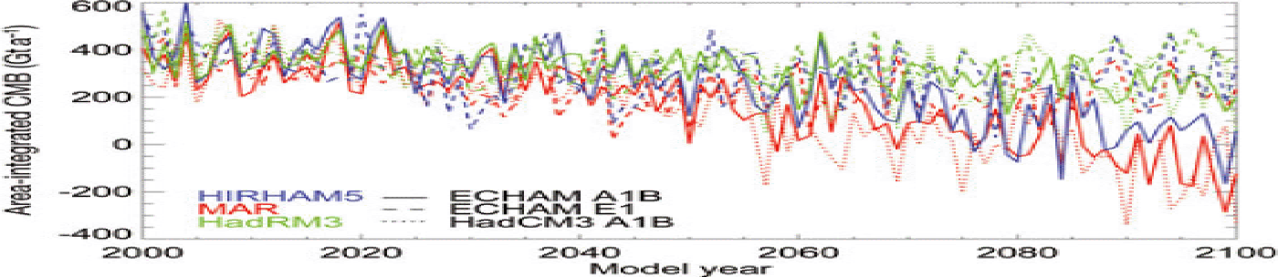
The forcing fields for the projection runs are created by adding anomaly fields, which are taken from the projected future climate, onto the present-day average climate from the ERA-Interim forced runs. The reason for using anomaly fields from the GCM-forced runs is that the average present-day climatic mass balance that results from forcing the RCMs with the two GCMs is smaller than the average balance from the ERA-Interim runs. Applying this GCM forced climatic mass balance to create a ‘Const init’ state results in an ice sheet that is only ~60% of the present-day ice-sheet volume and therefore not suitable as an initial state for the future simulations. The ‘Const init’ ice sheets resulting from forcing the model with the average climatic mass balance of either MAR or HIRHAM5 forced with ERA-Interim resemble the present-day ice sheet, whereas the ‘Const init’ ice sheet forced by ERA-Interim from HadRM3P does not. Therefore, we decided to use only the MAR and HIRHAM5 results that are forced with ERA-Interim to provide the initial model states and the present-day average climate for adding to the anomaly fields from the GCM-forced runs. The forcing fields used in the projection runs are thus generated by first subtracting the average present-day temperature and climatic mass-balance fields from each GCM scenario run and then adding these anomalies onto the average fields which have been forced by ERA-Interim from either MAR or HIRHAM5. This method of using scenario anomalies from GCM-forced runs is similar to that applied by Reference GoelzerGoelzer and others (2013). Figure 1 shows the area-integrated climatic mass balance over the RCM ice-sheet gridpoints after adding the ERA-Interim forced MAR averages to the anomaly fields of each GCM-forced run. From the MAR output, the area-integrated climatic mass balance over the ice-sheet gridpoints, averaged over 1989– 2010, is 377 Gt; from the HIRHAM5 output, in contrast, it is 491 Gt (averaged over 1989–2009, the period for which HIRHAM5 output is available). The simulations presented below assess how the chosen present-day climate will influence the projections.
The area-integrated climatic mass-balance fields computed over the ice sheet. Results from three RCMs forced with two GCMs and two emission scenarios are shown. The average present-day climatic mass balances from MAR forced with ERA-Interim (averaged over 1989–2010) have been added to the anomaly fields from the GCM-forced runs.
Results
Initialized ice-sheet model
The long ‘Paleo init’ initialization runs are done with 20 and 10 km grid resolution, and a 5 km simulation is regridded from the 10 km run 5 ka before the end of the run. Figure 2 shows the evolution of the total ice-sheet volume during the model initialization runs; it allows comparisons of the total volumes calculated for each initial ice-sheet geometry. The volume of the 20 km ‘Paleo init’ ice sheet exceeds that at 10 km resolution by ~15%. The models at 20 and 10 km resolutions fail to represent adequately the narrow marine-terminating outlet glaciers and properly to delineate the ablation zones and therefore are all ice-sheet projection runs performed at a 5 km model resolution. Model simulations with even higher resolution (2.5 and 2 km) show that the mass loss trends are consistent with respect to the grid resolution for horizontal grid spacings less than 10 km (Reference Aschwanden, Aðalsgeirsdóttir and KhroulevAschwanden and others, 2013).
Volume evolution during the ice-sheet model initializations. The ‘Paleo init’ state is developed by initialization runs from –125 ka BP up to the present, the ‘Const init’ by starting at the ‘Paleo init’ initial state and running for 60 ka, and the ‘FC init’ by taking the volume at –5 ka in the paleoclimate initialization run and continuing from that point to the present.
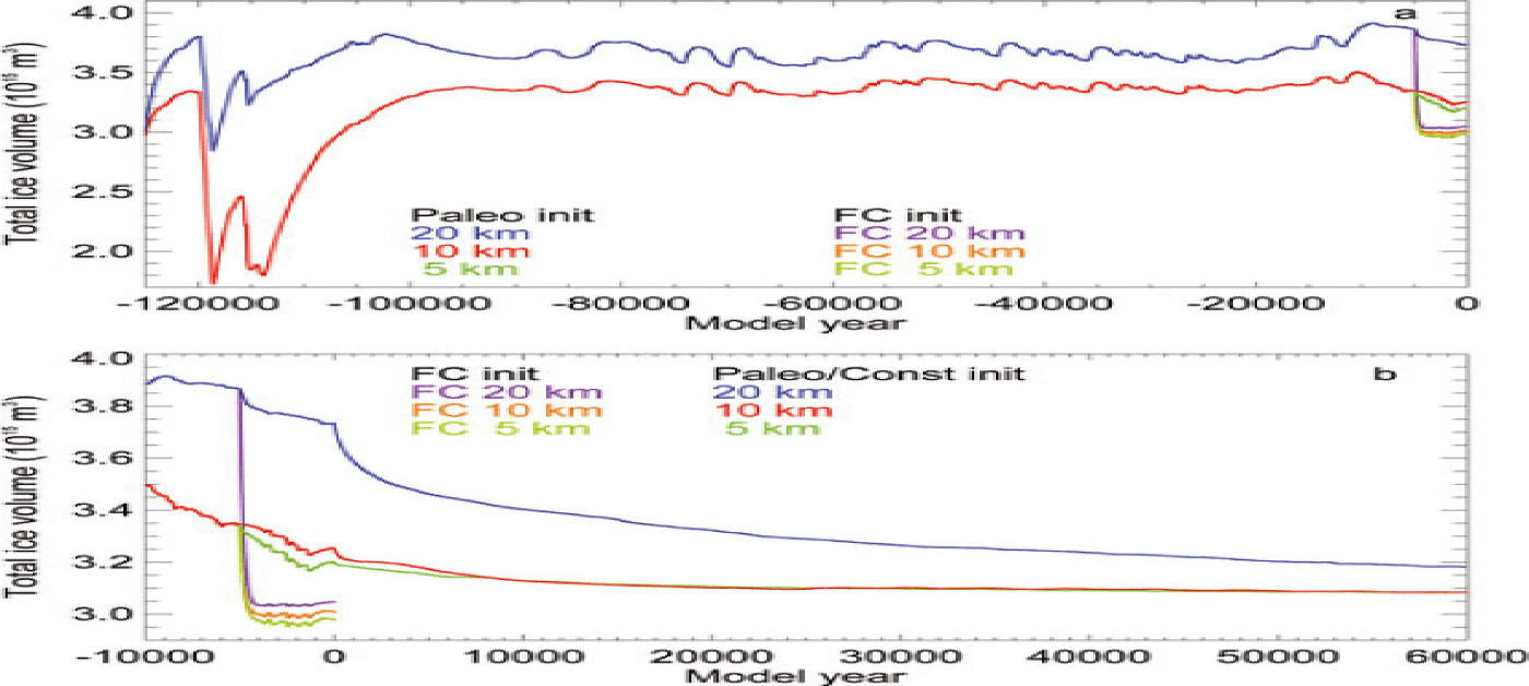
Figure 3 shows the topography and extent of the initial states, and Figure 4 presents three cross sections, which allow comparison of the ice thicknesses of the different initial states. Compared to the observed ice sheet, the ‘Paleo init’ and ‘Const init’ ice sheets are slightly thinner in their central and northwestern parts, while extending farther towards the north and southwest coasts and the steep areas on the east coast. The ‘Merged init’ ice sheet has the same shape as the ‘Const init’ sheet, and the ‘FC init’ sheet is very similar to the observed, as expected.
The 5 km resolution surface topography of the initialized ice sheets. (a) ‘Paleo init’, (b) ‘Const init’ and (c) ‘FC init’. The extent of the ‘FC init’ is the same as the observed ice sheet. The locations of the three cross sections selected for Figure 4 appear here as blue lines.

Three cross sections through the modeled initial states, at a 5 km resolution. The overhead locations of the cross sections are along the blue lines in Figure 3. Note the different scale on the x –axis in (c).

Projection runs
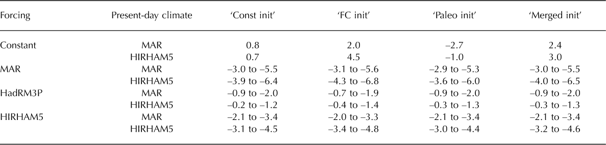
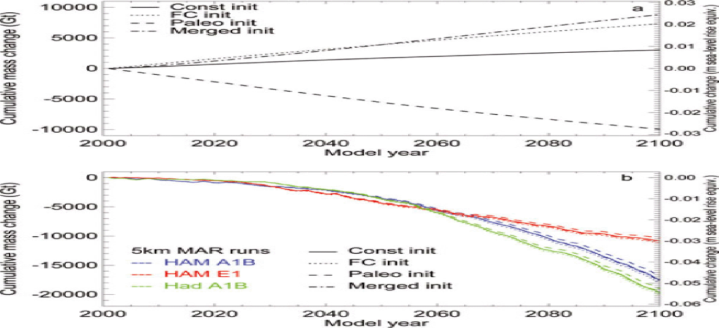
The model sensitivity to climate-forcing fields, the chosen present-day average climate and the initializing method can be assessed with the projection runs. In the projection runs, the initialization methods are likely to introduce drift while the model is recovering from the constraints imposed by the initialization procedure. The switch from a PDD scheme to climatic mass-balance forcing by the RCMs in the case of the ‘Paleo init’ state, the release of the mass-balance modifier in the case of the ‘FC init’ state, and the adjustment of ‘Merged init’ ice-sheet geometry to the new enthalpy field and basal conditions derived from the ‘Paleo init’ sheet are all processes that might introduce artificial drift into a scenario run. Therefore, 100 year runs from these initial states are done for comparison, in which constant average ERA-Interim climate fields from either MAR or HIRHAM5 are applied. The different cumulative mass balances during these runs are compared in the first two lines of Table 1. Note that the magnitude of drift is dependent on the applied present-day climate, and the drift of the ‘Paleo Init’ state is smaller when using HIRHAM5 present-day climate, but larger for the ‘FC init’ and ‘Merged init’ states. The time series of the drift caused by each of the four initialization methods during runs based on the MAR present-day climate are shown in Figure 5a, and Figure 5b shows the corresponding projections after subtracting the drift. The differences in cumulative mass change in Figure 5b are due to the different scenarios (A1B or E1) and the different GCM forcing fields (ECHAM or HadCM3). Between the two scenarios, the difference amounts to 1.9 cm sea-level rise equivalent, and between the GCMs to a difference of 0.6 cm sea-level rise equivalent. The forcings of the two scenarios result in different mass loss rates: under the E1 scenario the cumulative mass loss is greater by mid-century, but towards the end of the simulation period the mass loss computed with the A1B scenario has accelerated and results in a significantly larger sea-level rise contribution. This difference reflects the assumption made under the E1 scenario that successful reduction in carbon emissions through the 21st century has occurred.
Cumulative total mass balance (listed as sea-level rise equivalent (cm)) for model runs starting from the four initial model states as well as from the two constant average present-day climate fields (from MAR and HIRHAM5), forced with the output from the three RCMs indicated in the first column. The ranges are due to the different GCM and emission scenarios (ECHAM A1B or E1 and HadCM A1B). The time series in the third line under the column headings (MAR forcing, MAR present-day climate) are shown graphically in Figure 5, and the time series of the HIRHAM5 present-day climate runs at the bottom of the ‘Const init’ column are shown graphically in Figure 6
Sensitivity to the initialization method. (a) Changes in cumulative total mass during the constant forcing runs. (b) Scenario runs when the drift in (a) has been subtracted. All the runs in (a) and (b) start with the four initialized states and are forced with the MAR climatic mass balance, as forced by the average ERA-Interim. In (b), anomaly fields from the GCM-forced MAR runs are added to the forcing field. The varying colors refer to different GCM forcings and separate emission scenarios, and the variations in line style refer to the four initialization methods. The right-hand axis assumes an Earth ocean area of 36.1 × 10⁶ km2.
Similar values for the total cumulative mass balance during simulations with other combinations of present-day average climate fields and anomaly fields are shown in Table 1 and the ranges due to the initialization method, the GCM forcing fields and the scenarios in Table 2. When the present-day climate from HIRHAM5 is applied, there is a clear shift towards greater mass loss in the runs that use anomalies from HIRHAM5 and MAR, but towards smaller mass loss when anomalies from HadRM3P are used. There is also a greater sensitivity to the initialization method in the runs with present-day climate from HIRHAM5 and anomalies from HIRHAM5 or MAR (Table 2). There is no consistency as to which initialization method has the smallest or largest cumulative mass balance; the projections are similar in the initial 20–40 years but then start to diverge, and at the end of the 100 year simulation the difference is 5–15%. The sensitivity of cumulative mass change to the initializing method is smaller than the difference due to applied GCM or scenario (Table 2).
Ranges of cumulative total mass balance (listed as sea-level rise equivalent (cm)) for the different simulations. The ranges are due to the different initialization method, GCMs and emission scenarios (ECHAM A1B or E1 and HadCM A1B). The time series in the first line under the headings (MAR-forced, MAR present-day climate) are shown graphically in Figure 5b
The different RCM forcing fields lead to significant deviations in cumulative mass balance during the 21st century. Figure 6 presents examples of runs starting with the ‘Const init’ ice sheet created with the present-day climate from HIRHAM5 forced with ERA-Interim. In this figure, the drift occurring in the constant climate runs has already been subtracted. The ranges for the other simulations are shown in Table 1. The sea-level contributions during simulations forced with MAR anomaly fields are ~30% greater than from simulations forced with HIRHAM5 anomalies. The cumulative 21st-century mass loss from simulations forced by the HadRM3P anomalies is considerably smaller than from simulations forced by the MAR or HIRHAM5 anomalies. The reason is that HadRM3P does not simulate as much increase in surface melt (Fig. 1) because of its lower sensitivity to rising temperatures, compared to the other two RCMs. The differences among the RCMs stem primarily from varying approaches to simulating snow and ice melt, implementing surface albedo and representing refreezing processes; as a result, differences arise in climatic mass balance, despite the RCMs having the same lateral boundary forcing (Reference RaeRae and others, 2012). The interannual variability during individual scenario runs, however, is similar for all the RCMs (Fig. 1).
Sensitivity to climate forcing. Cumulative total mass balance of the ice sheet at a 5 km resolution, starting from the ‘Const init’ model state. The different colors refer to the particular RCM forcing fields, and the different line styles refer to the particular GCM and emission scenarios.
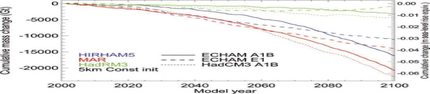
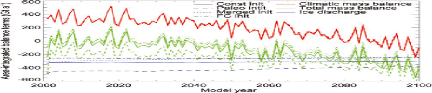
Figure 7 shows the integrated climatic mass balance, ice discharge (amount of ice calving at the margins) and total mass balance (the sum of climatic mass balance and ice discharge) for runs that begin with the four initial states and are forced with the MAR-ECHAM A1B scenario (using MARERA Interim as present-day average climate). As the figure demonstrates, the size and shape of each initial ice sheet results in different amounts of discharge from the margins. The smaller ice sheets, ‘Const init’, ‘FC init’ and ‘Merged init’, produce discharge amounts resembling the observed discharge of 325 Gta−1, obtained with the flux-gate method (Reference Rignot and KanagaratnamRignot and Kanagaratnam, 2006), while the larger ‘Paleo init’ ice sheet produces a discharge that is 30–40% greater, in line with the 1996–2008 estimate of 480–600 Gt a−1 (Reference Van den BroekeVan den Broeke and others, 2009). Although not demonstrated here, but shown in a hindcast simulation (Reference Aschwanden, Aðalsgeirsdóttir and KhroulevAschwanden and others, 2013), this agreement could be fortuitous, due to the model consistently overestimating the ice thickness and underestimating the ice flow. Also to be noted is that as the ice sheets decrease in volume over the 100 year projection run, the ‘Merged init’ and ‘Paleo init’ discharges decrease, while the ice discharges from the ‘Const init’ and ‘FC init’ remain nearly constant. This reduction arises from the modifications in ice-sheet shape that occur during the run.
Area-integrated climatic mass balance, ice discharge and total mass balance (sum of the climatic mass balance and ice discharge) for runs starting with the four initialized model states and forced with MAR-ECHAM A1B fields. Although the climatic mass balance over the ice sheet is the same for all the runs (red lines), the changing geometry of the ice sheets leads to slight deviations towards the end of the model runs. Ice discharge depends on the size and shape of the initial ice sheet (blue lines), and the differences in ice discharge impact the total mass balance (green lines). The differences in line style refer to the individual initialization methods.
Discussion
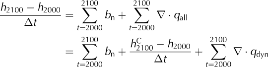
The elevation changes during the 100 year scenario runs ![]() are not only a direct effect of the climatic mass balance
are not only a direct effect of the climatic mass balance  but are also due to the dynamic developments (∇ ∙ qall) which include the elevation changes occurring during the constant-forcing runs (the drift,
  and other responses of the ice-sheet model, according to the continuity equation
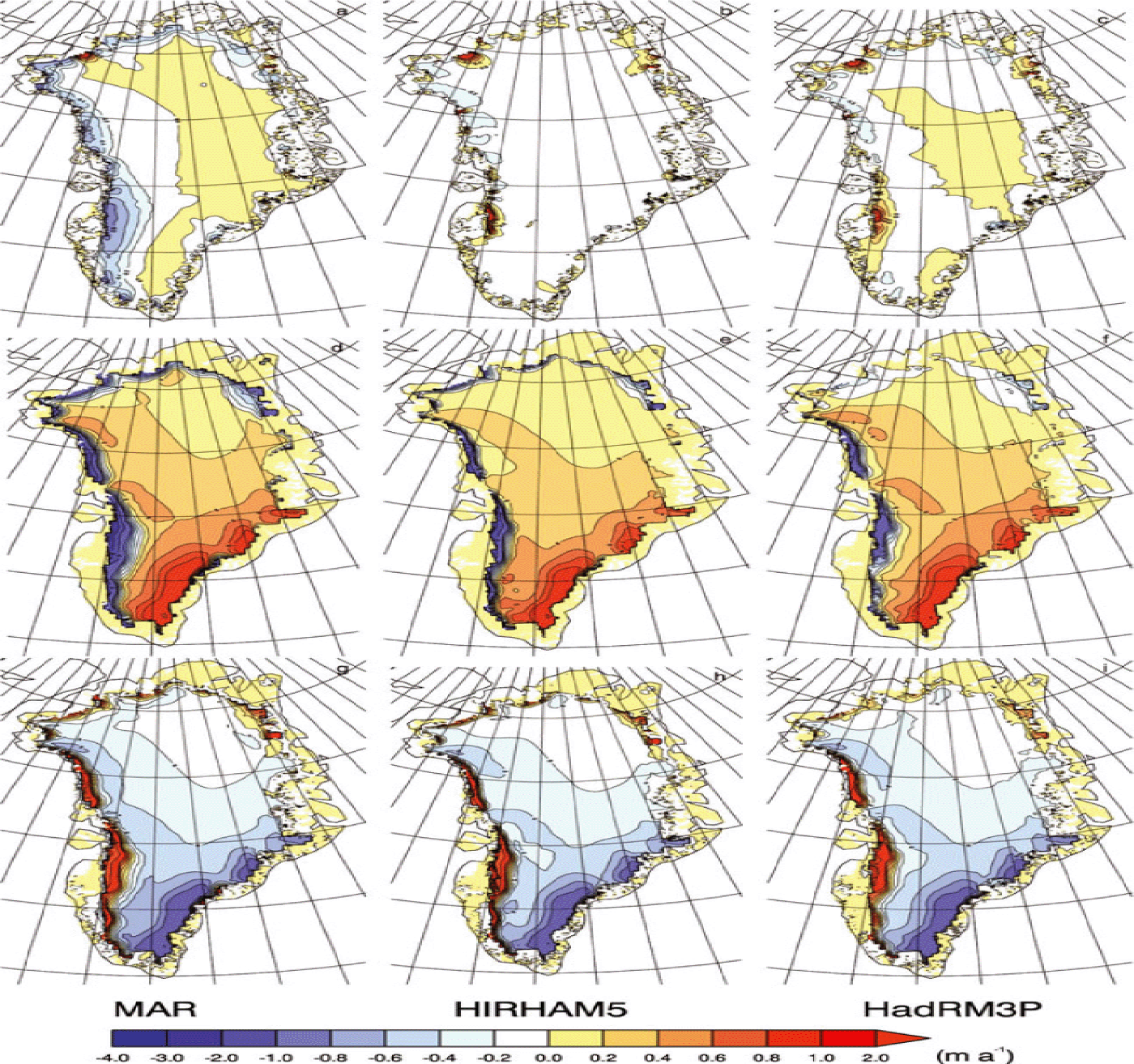
Figures 8 and 9 show these terms for the projection runs with different RCM forcings and different initial states, respectively. When the integrated climatic mass balance (Fig. 8d–f) and the elevation changes due to model drift (Fig. 9e–h), i.e. the first two terms on the right-hand side of Eqn (3), have been subtracted from the total 21st-century elevation changes, the remainder can be seen as the dynamic part  . The dynamic part represents the ice movement from the accumulation area to the ablation area. Numerous comparisons of this dynamic part, by starting runs from the different initial states and forcing them with anomaly fields from the different RCMs (Table 1), show that the dynamic parts remain remarkably similar. In 100 year simulations, the integrated difference over the entire ice sheet is sea-level rise equivalent of 2–3 mm. This confirms that the simulations are internally consistent, and highlights that for 100 year simulations the decisive forcing is that of climatic mass balance, as Reference GoelzerGoelzer and others (2013) concluded after experimenting with various dynamic model perturbations.
Surface-elevation changes forced with anomalies from the different RCMs (left column MAR, centre HIRHAM5, right HadRM3P). (a–c) Elevation change (h
2100 – h
2000)/Δt); (d–f) integrated climatic mass balance ; and (g–i) the dynamic part . All begin with the ‘Const init’ model state and are forced with the ECHAM A1B scenario and present-day average climate from MAR.
Surface-elevation changes during the 100 year projection runs starting from different initial states (from left to right: ‘Const init’, ‘Merged init’, ‘FC init’ and ‘Paleo init’). (a–d) Total elevation change (h
2100 – h
2000)/Δt) forced with the MAR-ECHAM A1B climate and MAR present-day average climate; (e–h) elevation change during runs with constant climate (the drift, ![]() ; and (i–l) the dynamic part which is the elevation change after the climatic mass balance and drift have been subtracted.
; and (i–l) the dynamic part which is the elevation change after the climatic mass balance and drift have been subtracted.
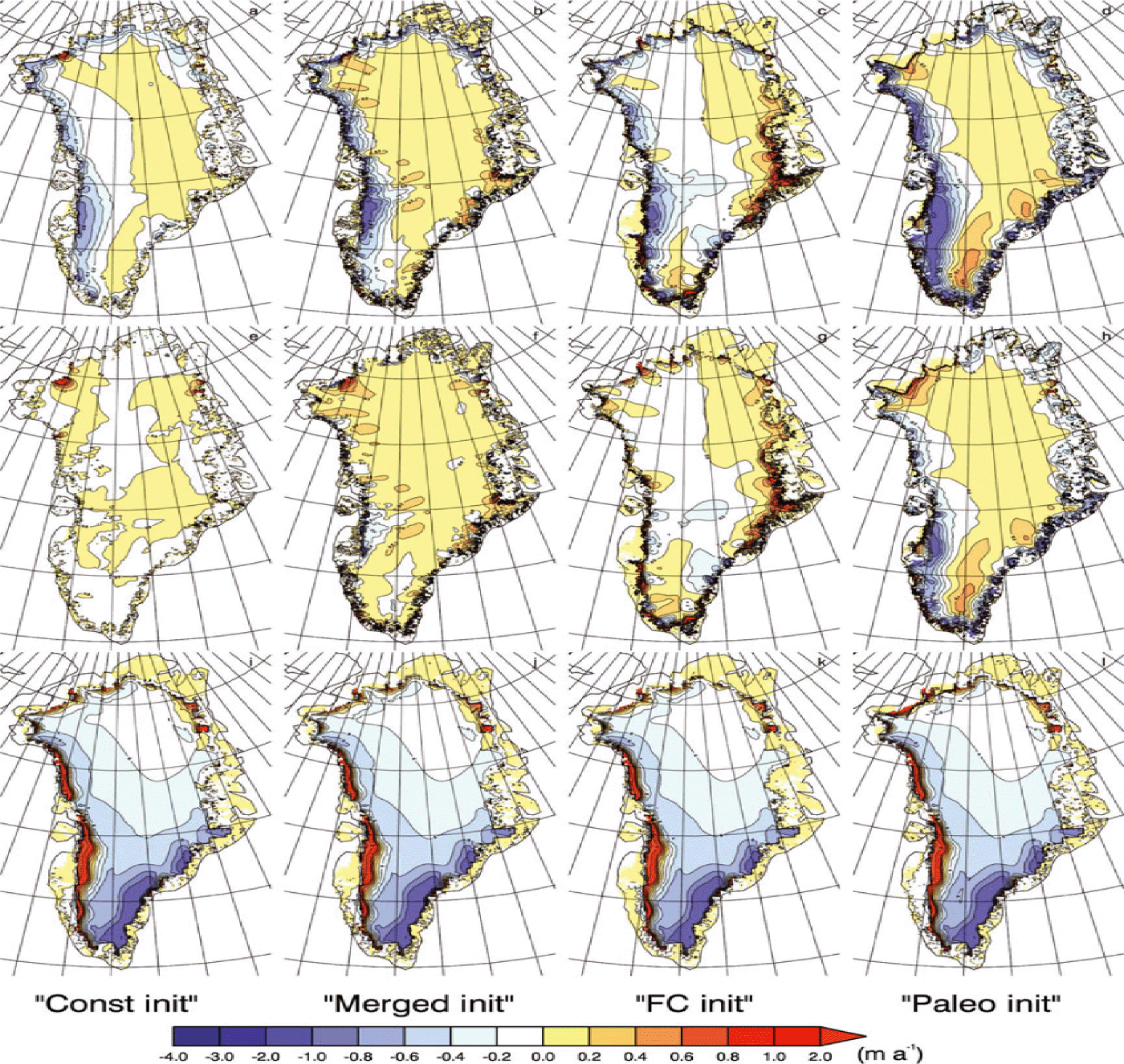
The elevation changes while forcing the model with the MAR RCM show that during the course of the 100 years, most of the interior area of the ice sheet thickens (Fig. 8a). In all the marginal areas and on the western and northern sides, however, the ice thins, except in the area around Petermann Gletscher in the northwest, where the elevation changes are positive. This is a mutual feature of all the simulations and can also be seen in the model-drift elevation changes (Fig. 9e–h). It appears that the combined ablation and ice discharge are smaller than the amount of ice transported towards Petermann Gletscher, yielding positive elevation changes there. As for elevation changes forced by the HIRHAM5 RCM (Fig. 8b), these are slightly negative for all of the interior area as well as most marginal areas, although the ice does thicken in the northwest and northeast and along the western margin southwards from Jakobshavn Isbræ. Finally, the elevation changes forced by the HadRM3P RCM share some basic features common to the other two RCMs, with the central area of the ice sheet, the northwestern corner, the western margin and the southeast region thickening, while the ice thins along the other margins. It therefore appears that the MAR and HadRM3P ice accumulations are more than able to compensate for ice flowing away from the accumulation areas. The ice thinning along the west coast in the MAR run demonstrates that the ice transport towards the west coast is unable to keep up with simulated ablation. In HIRHAM5 and HadRM3P, however, the simulated ablation amounts are smaller than the amount of ice transported towards the Jakobshavn area, resulting in ice thickening along this western margin.
With starting points in each of the four initialization states, the top row of Figure 9 shows the elevation changes ![]() during runs forced with anomaly fields from MAR-ECHAM A1B. Since the same integrated climatic mass balance is applied to all four initialization states, the differences in elevation changes reveal the varying dynamic contributions involved in the individual initialization methods. The middle row of Figure 9, on the other hand, presents the elevation changes during runs forced with constant climate , thereby spotlighting the adjustments which the model makes solely in relation to the initialization procedure. A comparison of the elevation developments in the two ice sheets with the same starting shape, ‘Const init’ and ‘Merged init’, reveals only slight differences due to contrasting enthalpy fields. The ‘Merged init’ ice sheet thickens across a broader central area than the ‘Const init’ ice sheet, as well as on the steep eastern margins, emphasizing that the colder, stiffer ice moves more slowly. At the margins, the total thinning rates of these two ice sheets are similar, with both thinning less than the integrated negative mass balance in the same area (Fig. 8d). This confirms that the dynamics of both ice sheets are favorable to efficient ice transport towards the margins, to replace the melted ice (Fig. 9i and j). While the thinning rates of the ‘FC init’ ice sheet at the western margin are similar to those of the ‘Const init’ and ‘Merged init’ ice sheets, indicating that the smaller ice sheets do not lose mass as fast as the ‘Paleo init’ ice sheet, it thickens along its whole eastern side. This thickening also occurs during the constant-climate simulation, indicating a strong response to the initialization method. In the hindcast experiment presented by Reference Aschwanden, Aðalsgeirsdóttir and KhroulevAschwanden and others (2013) the ‘FC init’ method produced unrealistic elevation changes compared to observations. This method of forcing the initialized ice sheet to be as close to observed ice thickness as possible appears to create unwanted transients in the projection runs. Compared to the other initial states, the ‘Paleo init’ model thins more in the marginal areas and thickens more across its central area, particularly on the south dome. This is a combined effect of the ‘Paleo init’ ice sheet being colder and stiffer and of the ice flow differences due to contrasting ice-sheet geometry.
during runs forced with anomaly fields from MAR-ECHAM A1B. Since the same integrated climatic mass balance is applied to all four initialization states, the differences in elevation changes reveal the varying dynamic contributions involved in the individual initialization methods. The middle row of Figure 9, on the other hand, presents the elevation changes during runs forced with constant climate , thereby spotlighting the adjustments which the model makes solely in relation to the initialization procedure. A comparison of the elevation developments in the two ice sheets with the same starting shape, ‘Const init’ and ‘Merged init’, reveals only slight differences due to contrasting enthalpy fields. The ‘Merged init’ ice sheet thickens across a broader central area than the ‘Const init’ ice sheet, as well as on the steep eastern margins, emphasizing that the colder, stiffer ice moves more slowly. At the margins, the total thinning rates of these two ice sheets are similar, with both thinning less than the integrated negative mass balance in the same area (Fig. 8d). This confirms that the dynamics of both ice sheets are favorable to efficient ice transport towards the margins, to replace the melted ice (Fig. 9i and j). While the thinning rates of the ‘FC init’ ice sheet at the western margin are similar to those of the ‘Const init’ and ‘Merged init’ ice sheets, indicating that the smaller ice sheets do not lose mass as fast as the ‘Paleo init’ ice sheet, it thickens along its whole eastern side. This thickening also occurs during the constant-climate simulation, indicating a strong response to the initialization method. In the hindcast experiment presented by Reference Aschwanden, Aðalsgeirsdóttir and KhroulevAschwanden and others (2013) the ‘FC init’ method produced unrealistic elevation changes compared to observations. This method of forcing the initialized ice sheet to be as close to observed ice thickness as possible appears to create unwanted transients in the projection runs. Compared to the other initial states, the ‘Paleo init’ model thins more in the marginal areas and thickens more across its central area, particularly on the south dome. This is a combined effect of the ‘Paleo init’ ice sheet being colder and stiffer and of the ice flow differences due to contrasting ice-sheet geometry.
The model drift during simulations that are forced with constant climate is shown in Figure 5a and the middle row of Figure 9. The drift in the simulation starting from the ‘Const init’ ice sheet is very small, only ~0.1% of the total volume. This residual drift indicates that in a mathematical sense the model is still not in a steady-state configuration even after 60 ka constant forcing, but the model is in a self-consistent state with the forcing field. The run starting from the ‘Merged init’ ice sheet results in a larger drift; the ice sheet expands as it adjusts its geometry to the enthalpy field and basal conditions of the ‘Paleo init’ ice sheet. The ‘Merged init’ ice is colder and thereby stiffer, due to its memory of temperatures during the Last Ice Age, and flows slower than the warmer ‘Const init’ ice. The simulated sea-level rise contributions of the two runs figure out to be the same, once the drifts appearing in the constant present-day climate runs have been subtracted (Fig. 5b; Table 1). This experiment setup does not separate the effect of model adjustments to the new enthalpy field, resulting from the initialization procedure, from the effect of slower response due to stiffer ice, which is a natural part of the drift and should be included in projections. Conclusions about whether the thermodynamic state in a Greenland ice sheet model will affect the response rate of the ice sheet over century-scale projections, as suggested by Reference Rogozhina, Martinec, Hagedoorn, Thomas and FlemingRogozhina and others (2011), or whether it is reasonable to use steady-state temperature profiles that do not include past climate history as Reference Seroussi, Morlighem, Rignot, Khazendar, Larour and MouginotSeroussi and others (2013) conclude, will have to wait for fully coupled runs over one or several glacial–interglacial cycles.
The projected sea-level rise from this model ensemble has a range from 0.2 to 6.8 cm sea-level rise equivalent, with the range arising from combined uncertainties in the initialization method (0.1–0.8 cm), the applied RCM (0.8–3.9 cm), GCM (0.4–0.6 cm) and scenario (0.65–1.9 cm) (Tables 1 and 2). The lower end of the range is due to the projections made with anomalies from HadRM3P, which has lower sensitivity to temperature increase than the other two RCMs (Reference RaeRae and others, 2012). These results are within the ranges of possible sea-level rise contribution from the Greenland ice sheet: 2–12 cm due to climatic mass balance and 1–6 cm due to dynamic-discharge changes under the SRES A1B scenario presented in the fifth assessment report of the Intergovern-mental Panel on Climate Change (Reference Church and StockerChurch and others, 2013). Similar to recent studies we find the largest uncertainty arising from the climate scenarios and the sensitivity of the climate models that derive the forcing (Reference Graversen, Drijfhout, Hazeleger, Van de Wal, Bintanja and HelsenGraversen and others, 2011; Reference GoelzerGoelzer and others, 2013; Reference Yan, Wang, Johannessen and ZhangYan and others, 2014).
The detailed response to climate forcing is clearly sensitive to the initial model state on a decadal timescale, as the initial size and shape (thickness and surface slope) of the ice sheet determine the driving stress and therefore the ice flow and mass loss through discharge. Furthermore, conclusions drawn from model simulations with a full force-balance model confirm that discharge and surface mass-balance anomalies cannot be treated independently, so a full coupling with local surface mass-balance models will be required to improve model predictive ability on centennial timescales (Reference Gillet-ChauletGillet-Chaulet and others, 2012). The four different initial states applied in this study respond differently to the applied forcing producing a model drift. In order to achieve drift-free model projections that fully couple the atmosphere with the ice sheet, the goal is for the initialization procedure to produce a model state with a similar size and shape to that of the observed ice sheet. Only such initial states will allow for projecting realistic ice discharges and for remaining self-consistent with the climate-forcing fields. One necessary factor in proper initialization will be a freely evolving ice surface, which can only be provided when climate models accurately represent the climate in Greenland without bias correction being required for the initialization procedure.
Conclusion
The method of initializing the ice-sheet model controls the size, shape and viscosity of the modeled ice sheet, which in turn determines the flow velocity and ice discharge. The model adjustment to the constraints imposed by the initialization method differs for the four methods tested here. The conclusion is that in order to realistically simulate future ice-sheet responses, the initialized ice-sheet model needs to be as similar to the currently observed ice sheet as possible, including the temperature field. At the same time it should remain fully self-consistent with climate forcing in order to minimize unnatural transients in the model response but maintain the natural response of the model which results from its initial state.
Two present-day (1989–2010) climate fields (MAR and HIRHAM5, forced by ERA-Interim) are used to create the initial states and to add to the anomalies for simulating the future. The model results presented here show that the projections are sensitive to the applied present-day climate. The drift in the runs with constant forcing varies according to the initial state of climate, resulting in a shift in the projections.
Ice-sheet responses involve a number of feedback mechanisms that can increase or decrease total volume loss. Although direct mass losses due to changes in climatic mass balance and to dynamic ice-sheet changes are included in our simulations, the impact that developments in surface elevation have on climatic mass balance is, for instance, not included, because the RCMs are run with a constant ice-sheet topography. Other feedback mechanisms not considered in this study include enhanced surface melt leading to enhanced basal lubrication and changes in ocean forcing effecting subglacial and frontal ablation at marine termini. Furthermore our study is limited to a small subset of parameters in both the ice-sheet and climate models. In order to account for all of the feedback mechanisms that may contribute to future volume changes in the ice sheet, it would be necessary to run a fully coupled ice-sheet– atmosphere model system. Therefore, the projected sea-level contribution presented here should be considered as the lower bounds for contributions from the Greenland ice sheet during the 21st century.
Acknowledgements
We thank Jennifer Griggs of Bristol University, UK, for providing updated 1 km topography grids for the Greenland ice sheet. Philip Vogler, of Lingua/Norðan Jökuls ehf., edited and clarified the text. The study received financial support from the Danish Agency for Science, Technology and Innovation, and is a part of the Greenland Climate Research Centre. PISM development is funded by a NASA Modeling Analysis and Prediction grant, NNX09AJ38G. This work was supported by funding for the ice2sea programme from the European Union’s Seventh Framework Programme (grant No. 226375, ice2sea contribution No. 101). This publication is contribution No. 48 of the Nordic Centre of Excellence SVALI, ‘Stability and Variations of Arctic Land Ice’, funded by the Nordic Top-level Research Initiative (TRI). A. Aschwanden was supported by NASA grant No. NNX13AK27G. We are grateful for comments and suggestions from Torsten Albrecht, three anonymous reviewers and the scientific editor, Ralf Greve, which helped to improve the paper.


