
11.1 Introduction
Climate, specifically Earth’s surface temperature, is controlled by solar insolation, albedo, and the greenhouse gas content in the atmosphere.Reference Sagan and Mullen1, Reference Walker, Hays and Kasting2 Solar insolation relates to the solar radiative flux, which depends on changes in the sun’s luminosity and the planet’s distance from the sun. Albedo represents the fraction of the solar radiative flux reflected back into space, which is influenced by clouds, ice sheets, vegetation, the land/ocean ratio, and aerosols. That part of the solar flux not reflected back into space is absorbed by Earth’s surface and re-radiated in the form of infrared energy. In the presence of certain gases that absorb infrared radiation, this re-radiated energy heats the atmosphere.
Radiative balance calculations show that, without greenhouse gases, Earth’s average surface temperature would be well below the freezing point of water.Reference Sagan and Mullen1 Geologic evidence for an active hydrologic cycle as far back as the early Archean suggests that Earth’s surface temperature has not strayed wildly from the triple point of water, requiring the warming effects of greenhouse gases. Even in the first 2 billion years, when the sun’s luminosity was substantially lower than today’s, surface temperatures were still conducive to liquid water. What is remarkable, then, is that the amount of greenhouse gases in the atmosphere must vary in a way that buffers Earth’s surface temperature, even when other factors like solar luminosity change. If greenhouse gases fall below some threshold, liquid water would freeze over globally, or if a threshold is exceeded, temperatures could rise to a level at which most of the water would be in the form of vapor, not unlike Venus today. This billion-year “stability” of Earth’s climate indicates that greenhouse gas contents are regulated by an internal thermostat to maintain a clement climate.Reference Walker, Hays and Kasting2
Superimposed on this billion-year climatic stability are shorter-term climatic fluctuations ranging from long-lived (10+ My) greenhouse and icehouse intervalsReference Berner3, Reference Zachos, Dickens and Zeebe4 to <100‑ky oscillations associated with Milankovitch orbital dynamics.Reference Hays, Imbrie and Shackleton5 Icehouse conditions of the last 30 My have been characterized by large, permanent polar ice sheets (Figure 11.1a) that wax and wane with orbital cycles.Reference Huybers and Wunsch6 In contrast, the late Mesozoic to early Cenozoic greenhouse interval (150–50 Ma) was characterized by average surface temperatures >10°C higher than today and free of permanent ice sheets (Figure 11.1a).Reference Zachos, Dickens and Zeebe4 Between 600 and 800 Ma, Earth may have temporarily experienced runaway icehouses, known as “Snowball” events, where temperatures got cold enough for continental ice sheets to develop at low latitudes.Reference Hoffman and Schrag7, Reference Hoffman, Kaufman, Halverson and Schrag8
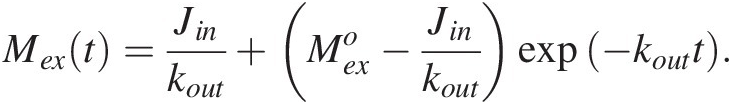
(a) Oxygen isotope record of seawater since 65 Ma with corresponding estimates of temperature on the right-hand axis (from Zachos et al.Reference Zachos, Dickens and Zeebe4). Onsets of Antarctic and northern hemisphere glaciations are shown. Box denotes the Paleocene–Eocene thermal maximum (PETM), which is expanded in (b). (b) Paleo-pCO2 estimates for the last 65 My (adapted from Zachos et al.Reference Zachos, Dickens and Zeebe4). (c) Carbon and oxygen isotopic composition of seawater across the PETM (adapted from Zachos et al.Reference Zachos, Dickens and Zeebe4). (d) Schematic diagram of the mass of C in the exogenic system (Mex) versus time. This diagram shows the concepts of response time (τ) and steady state.
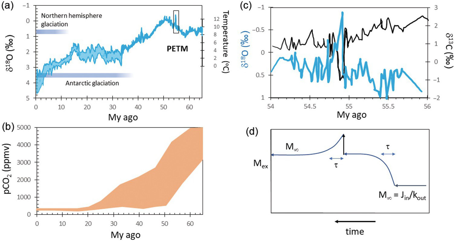
Paleo-proxy data indicate that the partial pressure of atmospheric CO2, the dominant greenhouse gas for most of Earth’s history, is generally high during greenhouse times and low during icehouses (Figure 11.1b).Reference Berner9, Reference Royer, Berner, Montanez, Tabor and Beerling10 Thus, understanding long-term climate variability requires an understanding of what controls the C content of the exogenic system, which we define here as the sum of the ocean, atmosphere, biosphere, and the thin veneer of reactive soil or marine sediments that support life (Figures 11.2 and 11.3). These exogenic reservoirs cycle rapidly between each other on timescales of days to thousands of years, allowing for short-term variability of atmospheric CO2. The exogenic C cycle operates on top of a much longer deep Earth C cycle, wherein the total amount of C in the exogenic system is controlled by fluxes into and out of Earth’s interior, which we term the endogenic system (Figures 11.2 and 11.3).
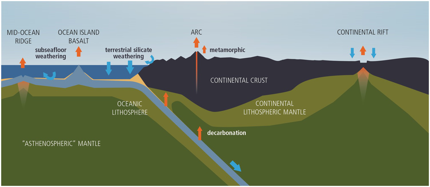
Cartoon (not to scale) showing how the whole-Earth C cycle relates to plate tectonics and the dynamics of the mantle. Orange arrows correspond to outgassing from Earth’s interior. Blue arrows correspond to carbonate precipitation or organic C burial. Curved blue arrows represent terrestrial silicate weathering and seafloor weathering.
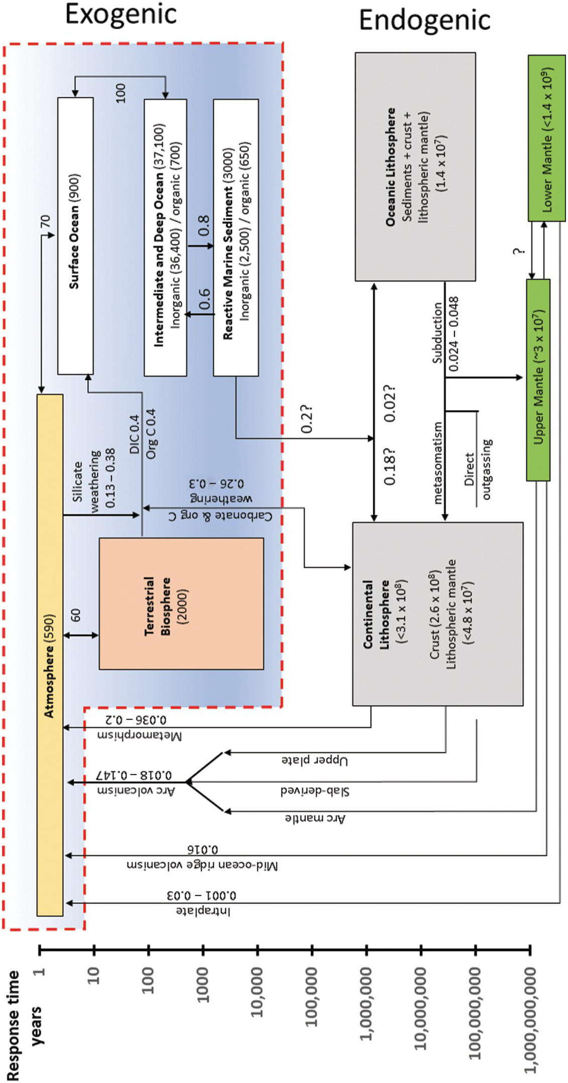
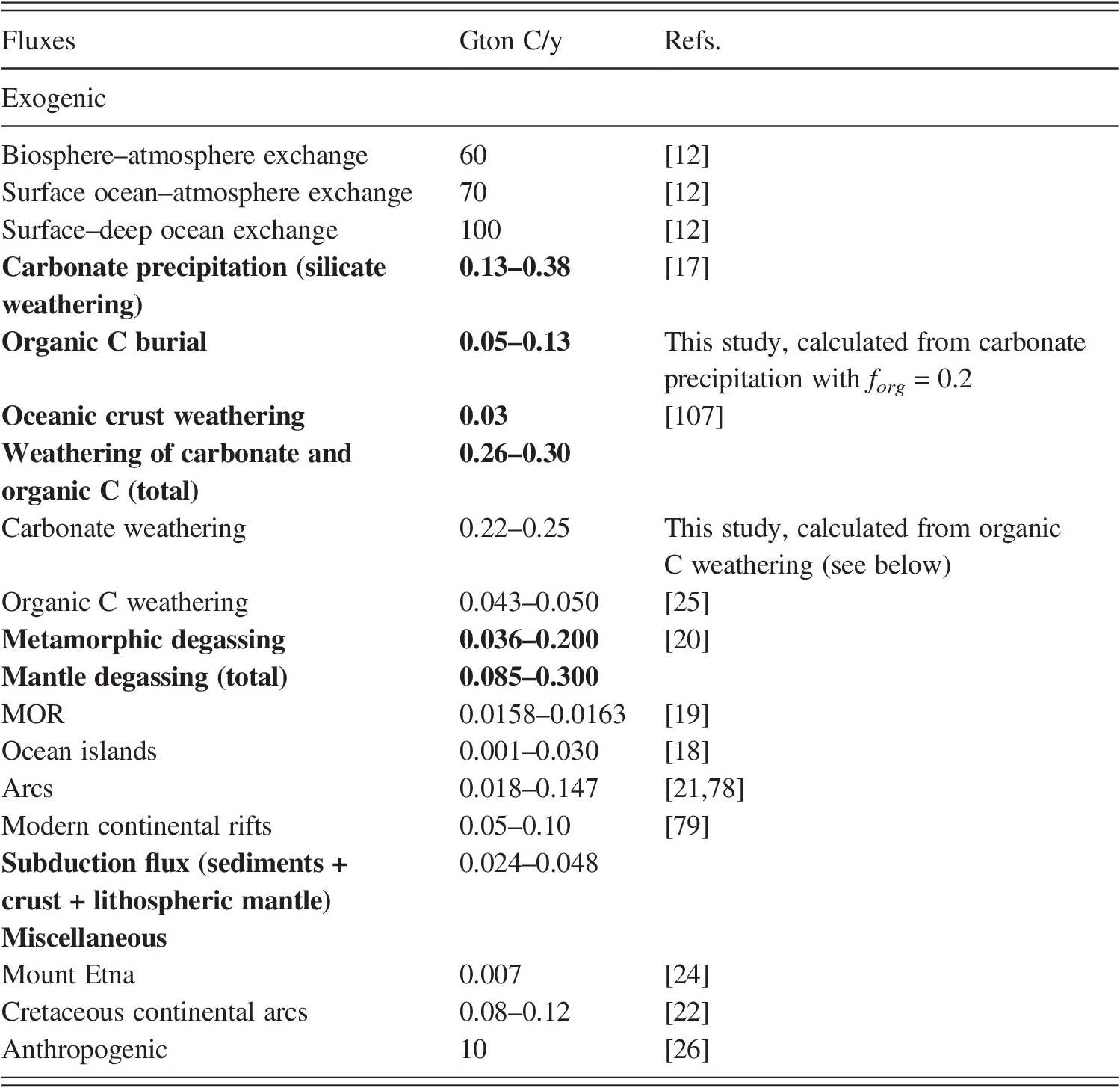
Box model describing the whole-Earth C cycle (excluding the core). Boxes within the red outlined region represent reservoirs within the exogenic system: the atmosphere, oceans, and the biosphere. All other boxes represent Earth’s interior reservoirs and refer to the endogenic system. Arrows represent fluxes of C from one reservoir to another. Numbers by arrows represent fluxes in units of Gton C/y. Numbers in parentheses within each box refer to total reservoir mass of C (Gton C). Reservoirs are placed according to the estimated residence or response time of C in the reservoir (see vertical axis). The vertical extent of each box represents the range of plausible residence/response times. The horizontal size of each box is arbitrary. Image inspired by Sundquist and Visser.Reference Sundquist and Visser11 C fluxes internal to the exogenic system are taken from Sundquist and Visser.Reference Sundquist and Visser11–Reference Hansell and Carlson16 Silicate weathering flux is taken from Gaillardet et al.Reference Gaillardet, Dupre, Louvat and Allegre17 Mantle degassing fluxes are from Dasgupta and Hirschmann,Reference Dasgupta and Hirschmann18 Tucker et al.,Reference Tucker, Mukhopadhyay and Gonnermann19 and other references discussed in the text. Metamorphic degassing data are from Kerrick and Caldeira.Reference Kerrick and Caldeira20 Volcanic arc emissions are from Burton et al.Reference Burton, Sawyer and Granieri21 Cretaceous continental arcs are from Lee et al.Reference Lee22 and Lee and Lackey.Reference Lee and Lackey23 Mt. Etna data are from Allard et al.Reference Allard24 Organic C weathering data are from Petsch,Reference Petsch25 from which carbonate weathering rates are calculated. Anthropogenic emissions are from Friedlingstein et al.Reference Friedlingstein26
The endogenic system includes C in the core, convecting mantle, and lithospheres (crust and lithospheric mantle). Endogenic C enters the exogenic system via volcanic degassing as well as metamorphic degassing and weathering of fossil organic C and carbonate. Carbon from the ocean, atmosphere, and biosphere is removed by carbonate precipitation and organic C burial, the former through an intermediate step of silicate weathering and the latter through photosynthesis. Subduction or deep burial of these carbonates and organic C is the mechanism by which exogenic C is transferred back into the endogenic system. The response time of the exogenic system to perturbations in C inputs or outputs is thought to be ~10–100 ky, which would imply that on My timescales, inputs and outputs are roughly balanced, so that the total exogenic C budget is near steady state.Reference Berner and Caldeira27, Reference Broecker and Sanyal28 The fact that Earth has fluctuated between long intervals of greenhouse or icehouse conditions implies that Earth transitions between different steady states, requiring that inputs from the endogenic system or the efficiency of weathering and organic C burial are not constant over My timescales. This chapter describes how C cycles between the endogenic and exogenic systems.
11.2 Basic Concepts of Elemental Cycling
11.2.1 Steady State and Residence Time
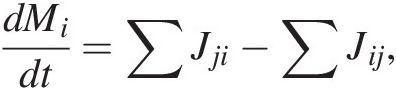
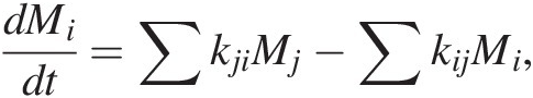
The rate of change of C mass in reservoir i, dMi/dt, is given by
 (11.1)
where the first term on the right represents the sum of all mass flows of C from reservoirs j into i and the second term right represents the sum of all mass flows of C out of reservoir i to reservoirs j. More simply, (11.1) expressed as total inputs Jin and outputs Jout from a reservoir M, such as the entire exogenic system Mex (ocean + atmosphere + biosphere), is given by
 (11.2)
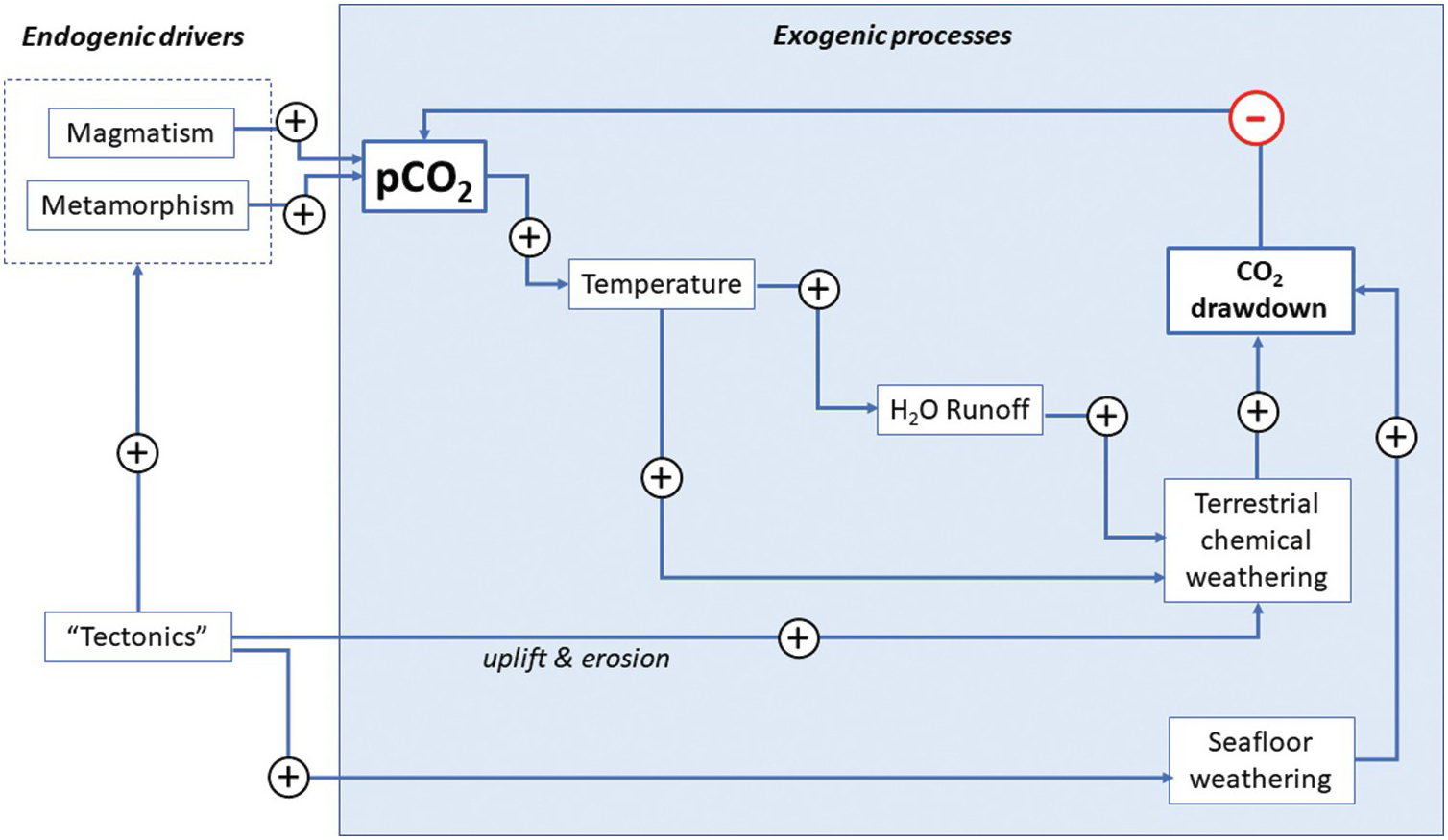
To completely model the CO2 content of the atmosphere (and not just the total exogenic system), both alkalinity and total C fluxes must be tracked, as the stoichiometry of these fluxes can vary considerably and their relative balance determines the proportion of exogenic C partitioned into the atmosphere. The treatment here, by ignoring this complexity, captures the first-order behavior of the system. Jin would then represent all inputs of C (volcanic and metamorphic degassing) and Jout the total C drawdown by silicate weathering (followed by carbonate burial) and organic C burial. Jout must scale with the amount of C in the system; after all, if there is no C in the exogenic system, then the output must be zero. At the most basic level, we can adopt a linear scaling, such that
where kout is the sum of all rate constants (s–1) describing the efficiency of different pathways by which C is sequestered from the exogenic system
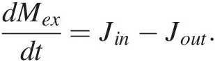
Analogous to radioactive decay, kout represents the probability that an atom of C is removed from the system per unit time. Because the output rate depends on the amount of C in the system, kout represents a negative feedback, which essentially counteracts any change in C in the system (see LasagaReference Lasaga29). As we will discuss later, kout represents a complex function of many processes. For example, C removal by silicate weathering and carbonate precipitation might be enhanced with greater water precipitation and temperature, both of which increase when atmospheric CO2 increases.Reference Walker, Hays and Kasting2 The net effect is a negative feedback (Figure 11.4).
Feedback loop describing the silicate weathering feedback acting on the exogenic C system. Arrows correspond to transfer functions, with positive symbols indicating positive feedback and negative symbols representing negative feedback. Increases in pCO2 increase temperature, which leads to enhanced precipitation and runoff, accelerating chemical weathering rates and drawdown of CO2. Similarly, an increase in pCO2 increases seafloor weathering rates, increasing drawdown of CO2. Tectonics and mantle dynamics drive the entire system by: (1) increasing erosion rates during mountain building, thereby increasing the availability of weatherable substrate and drawdown rates of CO2; and/or (2) increasing magmatic or metamorphic inputs of CO2 into the exogenic system. Whether tectonics enhance degassing or drawdown will depend on the nature of the tectonic activity.
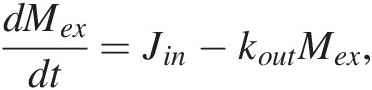
Jin must also scale with the mass of C from which the flux derives. If most of Jin derives from volcanic degassing, then Jin = kinMm, where Mm represents the mass of C in the mantle. If we assume that the mass of C in the mantle is much larger compared to that in the exogenic system, then Jin is approximately constant and (11.2) becomes a first-order differential equation:
 (11.5)
with the following solution:
 (11.6)
Here,  represents an initial perturbation to the amount of C in the exogenic system. Equation (11.6) shows that the system will return exponentially to a steady state, given by
 (11.7)
At steady state, inputs and outputs are balanced, hence the C content of the exogenic system does not evolve (steady state does not mean thermodynamic equilibrium). The time for the system to relax back to steady state after a perturbation (response time) is roughly the e-fold timescale of the system; that is:
For a linear feedback, the response time is equivalent to the residence time of C in the system (Figure 11.1d). The residence time represents the average time a C atom remains in the exogenic system when the system is at steady state, dMex∕dt = 0. At steady state, Jin = Jout, such that the residence time of C in the system is given by
 (11.9)
When negative feedbacks operate, a system perturbed suddenly, such as by a pulse of CO2 outgassing, will eventually return to a steady state, defined by the ratio of the external forcings (e.g. the input) to the efficiency of the negative feedback, kout (11.6). On timescales longer than the response time of the system, the C in the system should evolve toward a steady state, after which the only processes that can change the C content in the exogenic system would be temporal changes in the forcings, such as changes in magmatic or metamorphic activity, or changes in the efficiency of carbonate precipitation, which may relate to changes in tectonics and the efficiency of silicate weathering.
The response time for C in the exogenic system has been determined in two ways. One approach is to take the mass of C in the exogenic system and divide it by the measured inputs or outputs to obtain residence times. This approach is only valid if the measured inputs or outputs truly represent steady-state conditions. Another approach is to measure the relaxation time of a perturbed system, with one example being the C isotope excursion observed at the Paleocene–Eocene thermal maximum (PETM).Reference Zachos, Dickens and Zeebe4 Both approaches suggest that C in the exogenic system has a response time between 10 and 100 ky (Figure 11.1c and d).Reference Zachos, Dickens and Zeebe4 Thus, on My timescales, the C content of the exogenic system should be close to steady state. However, the fact that atmospheric CO2 nevertheless changes on My and Gy timescales means that tectonic/magmatic forcings or the global efficiency of the negative feedbacks must change with time as Earth evolves. In other words, Earth’s exogenic system is characterized by time-varying steady states or a baseline C content and climate. On short timescales, the exogenic system is not strongly influenced by the deep Earth, but on My timescales, the total budget of the exogenic C is controlled by the deep Earth through degassing and weathering.
11.2.2 Climatic Drivers versus Negative Feedbacks
The most important feature of negative-feedback systems is that steady state, if given enough time, will eventually be attained. Without a negative feedback, where the output does not depend on the amount of C in the exogenic system, a system is unlikely to attain steady state. In such a system, the C content of the exogenic system would rise indefinitely if inputs exceeded outputs or eventually decline to zero if outputs exceeded inputs. Earth’s climate has changed through time, but liquid water appears to have been present for almost all of Earth’s history, implying that inputs and outputs must be balanced on long timescales, which in turn implies that C in the exogenic system and climate is controlled by a negative-feedback mechanism. Any imbalances in inputs and outputs must be transient and occur on timescales shorter than the response time of exogenic C to perturbations (Figure 11.1d).Reference Berner and Caldeira27
Baseline or steady-state C in the exogenic system is driven by the inputs and modulated by the efficiency of the outputs. The greater the kinetic rate constant for C removal from the exogenic system, the more sensitive the negative feedback. In a steady-state system, this concept is illustrated well in a graph of C input or output versus total C in the exogenic system.Reference Caves, Jost, Lau and Maher30, Reference Kump, Arthur and Ruddiman31 For a linear system, the sensitivity of the negative feedback is the slope of the output as shown in Figure 11.5. Because the input of C from the deep Earth does not depend on the amount of exogenic C, the output function is represented by a horizontal line in Figure 11.5a. The intersection between the two lines defines the steady state. For a given sensitivity, k, the only way to change steady-state exogenic C is to change inputs. If inputs are instead held constant, exogenic C can only change by changing the strength (slope) of the weathering feedback. If exogenic C were to suddenly decrease below the system’s steady state, inputs would temporarily exceed outputs, returning exogenic C contents back to steady-state values. Conversely, if exogenic C contents were to suddenly increase, outputs would then exceed inputs, eventually returning the system to steady state. These concepts are shown in Figure 11.5b by keeping track of the intersection of the input and output functions. If the system were to become more efficient at C drawdown (higher k), such as if Earth was characterized by a global increase in mountain building and erosion, steady-state exogenic C would decrease. If drawdown efficiency were to decrease, such as through decreased weatherability of continents, steady-state exogenic C would increase without any change in the input (Figure 11.5b). Most importantly, if the negative-feedback efficiency is strong, then large changes in the inputs are required to change exogenic C, which is to say that the exogenic C content is buffered. This is why Earth’s climate, while variable over time, has rarely veered to extreme climatic conditions.
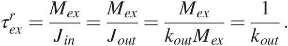
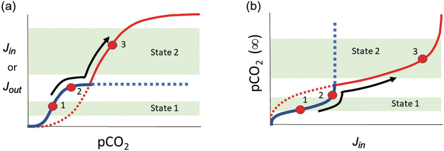
Inputs Jin and outputs Jout as a function of pCO2. Geologic inputs are assumed not to depend on exogenic C and are thus represented as horizontal lines. Output rate depends on pCO2, with the slope k representing the sensitivity of the negative weathering feedback. The intersection between Jin and Jout represents steady state, where Jin = Jout. The pCO2 at this intersection represents steady-state pCO2. In (a), we show that steady-state pCO2 increases by increasing Jin while holding the weathering feedback constant (red arrows from states 1 to 2 show an increase in steady-state pCO2). In (b), we hold inputs constant but decrease the sensitivity of the weathering feedback. This causes steady-state pCO2 to increase without any change in the input.
It is often debated whether Earth’s climate and exogenic C is input or sink driven. This debate is not about whether inputs or outputs are in balance because, on long timescales, they are in balance.Reference Zeebe and Caldeira32 The crux of this debate is whether changes in the C content of the exogenic system are controlled by changes in input or changes in the efficiency of the negative feedback (Figure 11.5). The former involve changes in magmatic, metamorphic, or weathering-related outgassing rates, while the latter involve changing the efficiency of weathering and organic C burial.
11.2.3 When Systems Transition to New Steady States
Despite the overall stability of Earth’s climate, there are examples when Earth or other planets have veered toward extreme climatic states. The Snowball climate of the Neoproterozoic, when Earth is thought to have frozen over, is an example of runaway cooling.Reference Hoffman, Kaufman, Halverson and Schrag8 Mars represents an example of a permanent icehouse, with surface temperatures of –55°C and no active hydrologic cycle.Reference Lodders and Fegley33, Reference Ingersoll34 Permanent greenhouse characterizes Venus, where surface temperatures are 460°C and the atmosphere is made of 96% CO2.Reference Lodders and Fegley33, Reference Ingersoll34 Earth itself may have undergone short-lived excursions to hothouse conditions. These include the PETM and the various hyperthermals around that time.Reference Zachos, Dickens and Zeebe4, Reference Dickens, O’Neil, Rea and Owen35, Reference Zachos, Pagani, Sloan, Thomas and Billups36
In a linear system, runaway processes cannot happen. However, negative-feedback mechanisms need not scale linearly with exogenic C content. For example, if the rate-limiting step for silicate weathering and precipitation of carbonates becomes the rate at which fresh new rock is exposed to the atmosphere, one could envision a “threshold” of atmospheric CO2 content above which further increases in CO2 do not result in increased weathering. Similarly, a scenario could be envisioned in which surface temperatures drop to a threshold below which weathering kinetics become negligible, and because surface temperature is in part controlled by the amount of greenhouse gases, this translates to a threshold of atmospheric CO2 below which weathering rates are insensitive to CO2. Thus, the functional form for the negative feedback might involve low-sensitivity regimes at low and high atmospheric CO2 separated by a sensitive, quasi-linear regime at intermediate CO2 contents (Figure 11.6). For a scenario in which C inputs to the exogenic system do not depend on atmospheric CO2, one can track how steady-state exogenic C varies as inputs vary. From Figure 11.6, we see that when inputs rise toward an upper threshold, steady-state exogenic C contents can rise uncontrollably, leading to a runaway greenhouse. If inputs decrease below some lower threshold, steady-state exogenic C contents will plummet, resulting in runaway icehouse conditions. Crossing these thresholds may move the planet to a different steady state, where a new type of negative feedback operates (Figure 11.7). Understanding the functional form of global weathering feedbacks is thus critical to understanding where these thresholds lie in terms of exogenic C.
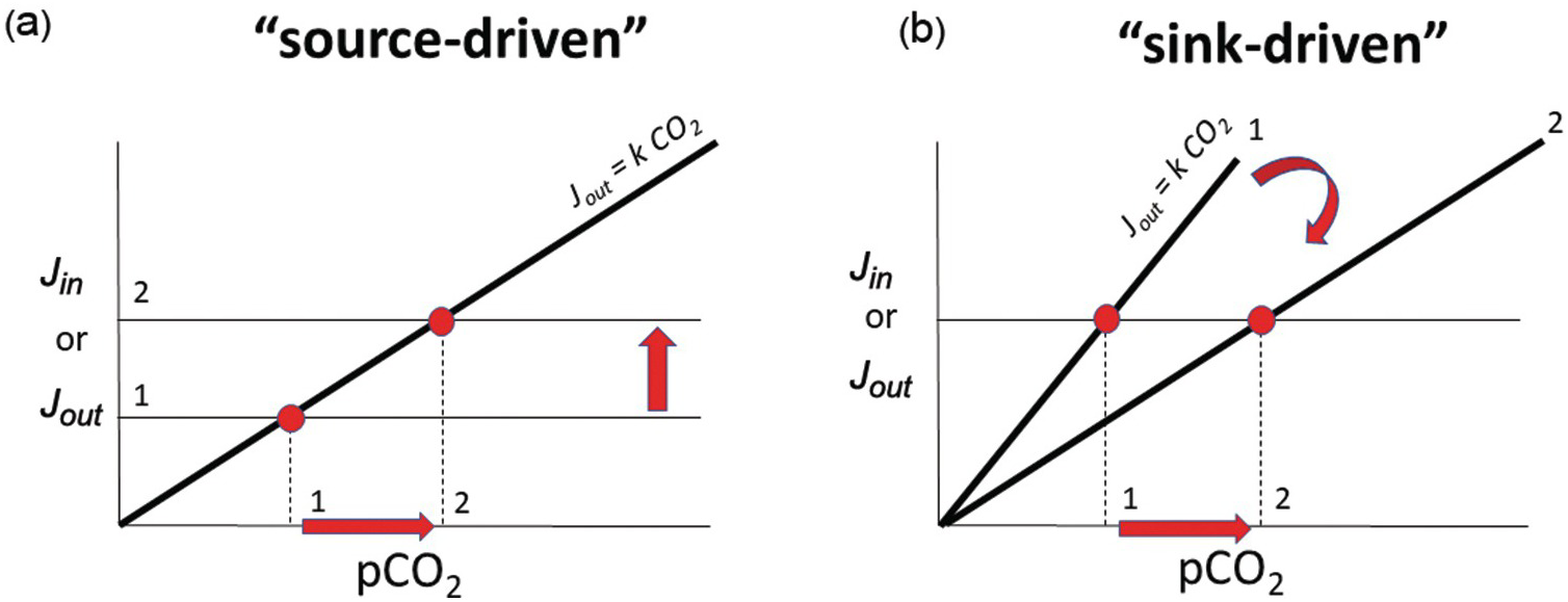
(a) Input Jin and output Jout versus pCO2. The conceptual model is identical to that of Figure 11.5, but the functional form of the weathering feedback Jout is nonlinear, consisting of low-sensitivity regimes at low pCO2 and high pCO2. These low-sensitivity regimes are referred to here as kinetically limited and substrate-limited, respectively. At low pCO2, temperatures are low and kinetics of dissolution are sluggish. At high pCO2, reaction is limited by the availability of new substrate for weathering. Between these two low-sensitivity regimes lies a quasi-linear high-sensitivity regime, where climate is stable. Intersections of Jin (thin horizontal lines) with Jout (thick bold line) are denoted by red circles. (b) Steady-state pCO2 in (a) is plotted versus Jin. When inputs rise to some threshold (e.g. from states 1 to 2), further increases in Jin will lead to rapid rises in pCO2. Conversely, when inputs drop below some threshold (states 1 to 3), further decreases in Jin will lead to rapid declines of pCO2. Hothouse and icehouse excursions are controlled by how close the system’s baseline climate is to the threshold.
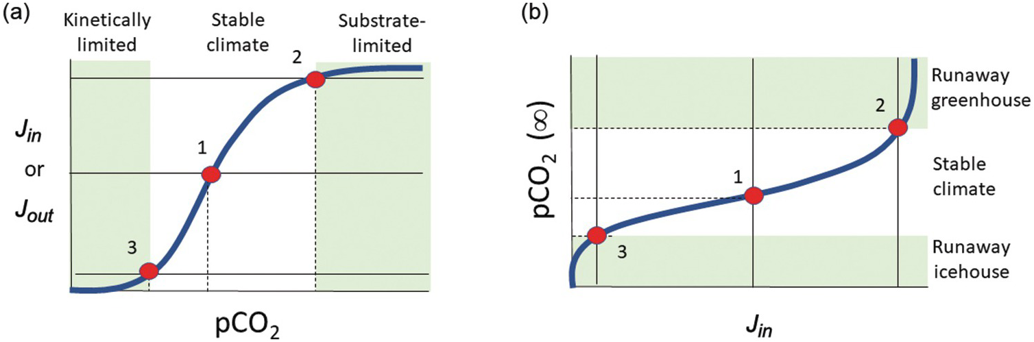
(a) and (b) are schematic diagrams that are conceptually identical to those of Figure 11.6, except that two different functional forms of the weathering feedback Jin are shown. The two different weathering feedback mechanisms are assumed to operate at different pCO2 values such that the system can transition into a fundamentally new state after it crosses a pCO2 threshold (e.g. from states 1 to 2 to 3).
11.3 Carbon Inventories of Earth Reservoirs
11.3.1 Modern and Primitive Mantle Reservoirs
Excluding the core, more than 99.99% of all C on Earth is in the mantle and crust, although exact quantities are highly uncertain.Reference Dasgupta and Hirschmann18 Estimates of the C budget of the uppermost mantle are indirectly calculated from the C content of mid-ocean ridge basalts (MORBs), with C itself inferred by bootstrapping to other elements, such as Nb, Ba, H, or noble gases.Reference Saal, Hauri, Langmuir and Perfit37–Reference Marty and Jambon39 These studies have resulted in estimates of 16–300 ppm C for the MORB source mantle, typically assumed to represent the upper mantle (Figure 11.3). However, reconstructing mantle C contents is faced with the challenge of correcting for degassing of C and other elements. Tucker et al.Reference Tucker, Mukhopadhyay and Gonnermann19 and Hauri et al. (Chapter 9 of this book) provide the most recent and rigorous reconstructions of the MORB source region and arrive at 30 ppm C (Table 11.1). This estimate agrees well with previous estimates of ~15–50 ppm C for the MORB source mantle that used undegassed or minimally degassed MORB CO2 contents and CO2/Ba, CO2/Nb, and H/C ratios (e.g. Refs. Reference Saal, Hauri, Langmuir and Perfit37, Reference Hirschmann and Dasgupta38, Reference Michael and Graham40, and Reference Rosenthal, Hauri and Hirschmann41). A homogeneous upper mantle (<670 km; mass of 1.06 × 1024 kg42) with a MORB source C content would contain ~3.2 × 10⁷ Gton C (Figure 11.8). If the MORB source was representative of the entire mantle down to the core–mantle boundary (4.0 × 1024 kg), the whole mantle would contain 1.2 × 10⁸ Gton C.

BSE = bulk silicate Earth; DM = depleted mantle; ROL = recycled oceanic lithosphere.
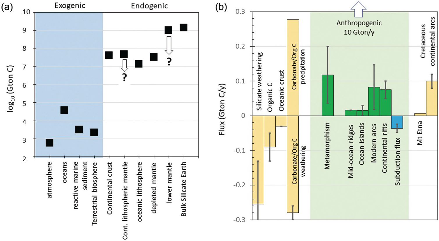
(a) Estimates of total C content (Gton C) in various exogenic and endogenic reservoirs. See Table 11.1 and text for details. Estimates of the continental lithospheric mantle and bulk silicate Earth (BSE) are from this study. Downward-pointing arrows denote that these estimates represent maximum bounds. Depleted mantle volume corresponds to mantle above 670 km with C concentration equal to that inferred for the MORB mantle source. Lower mantle corresponds to mantle between 670 km and the core–mantle boundary with a C concentration equivalent to BSE. (b) Graphical representation of C fluxes (Gton C/y) with inputs as positive values and outputs as negative values. Silicate weathering, organic C burial, and seafloor weathering are shown in yellow. Inputs of CO2 via weathering of organic C and carbonates are combined (negative bars), but such weathering is thought to be balanced by rapid re-precipitation of carbonate and burial of organic carbon (positive bars). Endogenic outgassing is shown in green, while subduction is shown in blue. Degassing through Mt. Etna and Cretaceous continental arcs is shown in order to illustrate the importance of carbonate-intersecting continental arcs. Vertical arrow points to anthropogenic production of CO2 through fossil fuel burning and cement production (10 Gton C/y).
Of interest is the C content of the bulk silicate Earth (BSE), which is the primordial mantle prior to extraction of the continents, oceans, and atmosphere (Figure 11.9a). The present mantle represents what remains of the mantle after degassing and silicate differentiation, which we refer to as the Depleted Mantle (DM); the composition of the DM is assumed to be represented by the MORB source mantle.Reference Hofmann43, Reference Zindler and Hart44 Thus, the BSE can be calculated by re-homogenizing the atmosphere, oceans, and continents back into the DM, but this is challenging if the C contents of all of these reservoirs and their sizes are not known well. A common approach, used for refractory lithophile elements, is to extrapolate magmatic differentiation trends to chondritic ratios, but this cannot be done for C because of its volatility during nebular condensation/planetary accretion and siderophile nature during core formation (e.g. Ref. Reference Chi, Dasgupta, Duncan and Shimizu45).
(a) Cartoon showing how C concentration in BSE is determined. BSE is the hypothetical primordial mantle composition after combining the DM, continental crust (CC), continental lithospheric mantle (CLM), and all other reservoirs, such as recycled oceanic lithosphere (ROL), as well as oceans, atmosphere, etc. (latter not shown because of small size). (b) C content of BSE as constrained by relative depletion of Ba and U in DM. Horizontal axis represents the relative efficiency k by which C is retained (during melting) or recycled (during subduction) into the mantle compared to Ba or U; k is likely larger than 1. (c) Missing fraction of C from the DM after subtraction of C in continental crust (DM is assumed to be the size of the upper mantle down to 670 km). Thick black lines correspond to estimates based on C/Ba-constrained BSE and thin blues lines are based on C/U-constrained BSE. Two sets of lines for each color are denoted and correspond to calculations using the crustal budgets of C from WedepohlReference Wedepohl58 and Gao et al.Reference Gao59 This missing C can be stored in the CLM or as recycled components in the mantle. (d) Maximum concentration of C in CLM, assuming all missing C is the CLM.
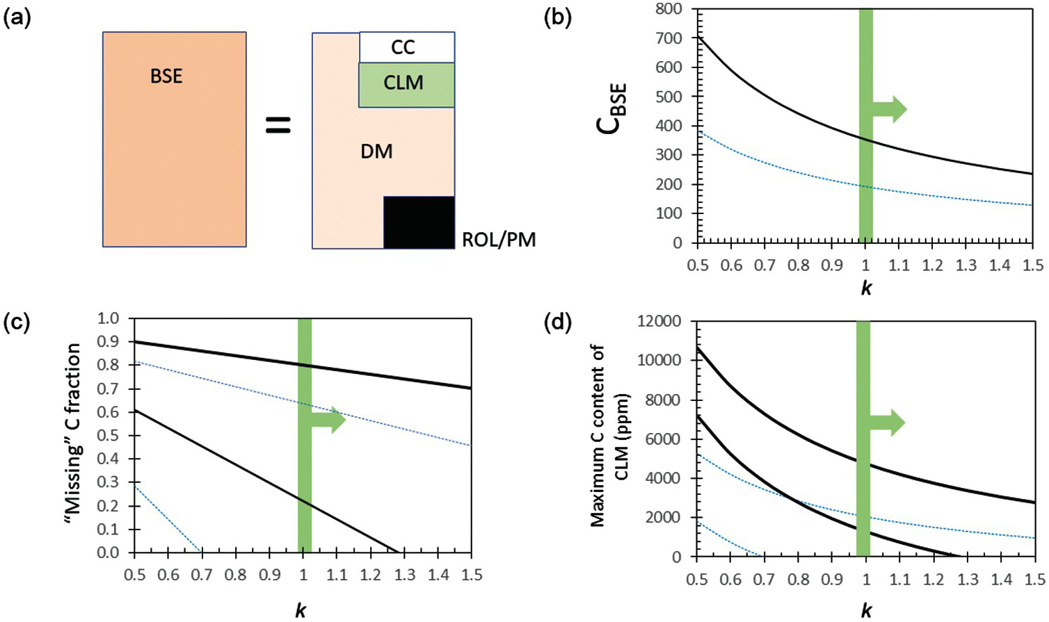
Instead, we infer the C of BSE from elements that behave geochemically like C but are refractory in a cosmochemical sense. For example, during mantle melting, C is thought to behave like Ba, a refractory element.Reference Tucker, Mukhopadhyay and Gonnermann19, Reference Rosenthal, Hauri and Hirschmann41 The depletion of Ba in the DM (0.563 ppmReference Workman and Hart46) relative to the BSE (6.6 ppmReference McDonough and Sun47) – that is, BaDM/BaBSE – is ~0.085. If Ba and C also behave similarly during subduction, then the relative depletion of C in the MORB source is equivalent to that of Ba. The BSE concentration of C is then calculated by dividing the C concentration of the DM by the Ba depletion factor (CBSE = CDM/(BaDM/BaBSE)), yielding ~350 ppm C for the BSE (Figure 11.9b). If C does not behave identically to Ba, then a correction factor must be applied, CBSE = CDM/(kC/Ba × BaDM/BaBSE), where kC/Ba represents the efficiency by which C is returned to the mantle relative to Ba (or the relative efficiency by which C is retained or recycled into the mantle relative to Ba). If kC/Ba > 1, C is preferentially subducted deep into the mantle relative to Ba and our estimates of C in the BSE are hard maximum bounds. If kC/Ba < 1, Ba is preferentially recycled and our estimates are minimum bounds (Figure 11.9b). It seems likely that Ba, mostly concentrated in slab sediments, is more efficiently removed from the subducting slab given the extreme enrichments of Ba in arc lavas.Reference Elliott, Plank, Zindler, White and Bourdon48 While some of the carbonate in subducting sediments might also be removed efficiently,Reference Kelemen and Manning49 organic C and carbonate in the oceanic crust are likely retained,Reference Duncan and Dasgupta50, Reference Dasgupta51 so it seems likely that kC/Ba > 1, and thus CBSE < 350 ppm. If C during melting behaves more like U, a refractory element with a DM depletion factor of ~0.16 relative to BSE (Figure 11.9b),Reference Workman and Hart46 CBSE < ~192 ppm. In any case, CBSE can be no higher than <350 ppm (Table 11.1), consistent with a recent estimate of CBSE of ~140 ppm.Reference Hirschmann52 These values of CBSE would imply that the DM reservoir has lost no more than 40–90% of its original C during silicate differentiation; however, the DM reservoir is unlikely to represent the entire convecting mantle, so the fractional loss of C from the whole mantle must be far smaller. We note that the C concentration of the mantle source of ocean island basalts (OIBs) ranges from 33 to 500 ppm C.Reference Dasgupta and Hirschmann18 The source region of OIBs is thought to represent primitive undegassed mantle and/or enriched domains associated with recycled crust.Reference Hofmann and White53, Reference Garapić, Mallik, Dasgupta and Jackson54
11.3.2 Continental Crust and Continental Lithospheric Mantle
Carbon in the continental crust is represented by ancient sedimentary rocks as well as carbonate and graphite stored in metamorphic and igneous basement rocks. The sedimentary rocks are dominated by carbonates (limestones and dolostones) with organic C-rich sediments making up a smaller fraction.Reference Wilkinson and Walker55, Reference Wilkinson and Algeo56 The carbonate content of the continental crust is calculated by estimating the volume of carbonate sediments in the continents.Reference Ronov57, Reference Wedepohl58 Due to high variability in the organic C content of sediments, the average organic C content of continents is usually estimated by assuming that organic C makes up ~20% of the total C budget. This approach is based on the assumption that the C isotopic composition of seawater, often assumed to represent the fraction of organic C (forg), has remained relatively constant over most of Earth’s history. The C content of the rest of the continental crust is estimated from measurements of basement rocks and extrapolated to the upper, middle, and lower crusts based on a model of the compositional structure of the crust. Because of the high degree of variability in carbonate content of igneous and metamorphic rocks, any estimate of the C content of the nonsedimentary part of the continental crust is fraught with large errors. For example, WedepohlReference Wedepohl58 estimated that the continental basement amounted to one-fifth of the C in sedimentary rocks, yielding a total continental crust budget of 4.2 × 10⁷ Gton C. A more comprehensive study of basement rocks in China found higher concentrations of C in igneous and metamorphic rocks, leading to a much higher estimate of the total continental crust budget of 2.6 × 10⁸ Gton C.Reference Gao59
We now turn to the continental lithospheric mantle (CLM), the cold and hence rheologically strong part of the mantle underlying the continental crust, which extends down to depths of ~100 km beneath Phanerozoic terranes and up to ~200–250 km beneath many stable cratons.Reference Jordan60–Reference Gung, Panning and Romanowicz63 Because of their Gy stability,Reference Pearson64–Reference Walker, Carlson, Shirey and Boyd67 CLM is subjected to numerous metasomatic events, which could lead to hydration or carbonation.Reference Foley68–Reference Dasgupta75 We can place an upper bound on how much C could be in the CLM. If we assume that the volume of DM is equivalent to the entire upper mantle down to 670 km depth (1.06 × 1024 kg), the total amount of C degassed is <3.4 × 10⁸ Gton C as inferred above from C/Ba systematics and >1.7 × 10⁸ Gton C from C/U systematics. From these quantities we subtract the amount of C in the continental crust. If we use the higher crustal abundances of Gao et al.Reference Gao59 and the DM C content inferred from C/Ba, we are left with 20% of unaccounted C that must be housed in the CLM or as recycled components deep in the mantle (Figure 11.9c). If we use the crustal abundances of Wedepohl,58 80% is unaccounted for. If we use the lower estimates of C in DM as inferred from C/U systematics, we find that the C budget of the continental crust accounts for or even exceeds the amount of C degassed from the upper mantle, which seems unreasonable; reconciling this discrepancy would require a volume of mantle greater than the upper mantle to have degassed to the extent of the DM reservoir. In any case, if we restrict the DM to the upper mantle and use the C/Ba-constrained DM composition and Gao et al.’s crustal estimate, we find a maximum missing C of 4.8 × 10⁷ Gton C. All of this C in the CLM would translate to a hard upper bound of ~740 ppm C in the CLM, assuming an average CLM thickness of ~150 km (Figure 11.9d and Table 11.1). No doubt, some of the missing C is in the form of recycled crust deep in the mantle, as balancing present-day arc flux requires a small fraction of subducted C to be supplied to sub-arc mantle source regions via fluids or melts (e.g. Ref. Reference Duncan and Dasgupta76). Whether the missing C is in the CLMReference Kelemen and Manning49 or recycled into the deep mantleReference Hirschmann52 is currently debated.
11.3.3 Exogenic Reservoirs
For completeness, we briefly discuss the C budget of the exogenic system (Table 11.1). In total, the exogenic system accounts for <0.01% of Earth’s C budget (excluding the core), with reservoir sizes increasing as follows (Figure 11.3): atmosphere < terrestrial biosphere and soil < reactive marine sedimentary carbon < ocean.Reference Sundquist and Visser11 For a modern preindustrial atmospheric CO2 content of 280 ppmv, the total amount of pre-anthropogenic C in the atmosphere today is 590 Gton or ~1.4% of the total C in the exogenic system.Reference Sundquist and Visser11 The oceans account for ~87% of the total exogenic C, with most of the C in the oceans in the form of HCO3–. The terrestrial biosphere and soils account for ~4% and the reactive marine sedimentary reservoir accounts for ~8% of the total exogenic C. It is possible that the reactive marine sedimentary reservoir is substantially larger than noted here if the size of gas-hydrate reservoirs has been underestimated.Reference Dickens77
In summary, although the amount of C in the exogenic system is nearly negligible compared to that of the bulk Earth, all C degassed from the interior of Earth passes through the exogenic system before being buried as carbonates or organic C, and it is through the exogenic system that C influences climate.
11.4 Long-Term Carbon Fluxes
11.4.1 Inputs
11.4.1.1 Volcanic Inputs
On long timescales, the exogenic system is supported by C inputs from the endogenic system through volcanism, metamorphism, and weathering of ancient carbonates and organic C. Outputs from the exogenic system occur through carbonate and organic C burial via the intermediate steps of silicate weathering and photosynthesis. Ultimately, some fraction of carbonate and organic C is removed from the exogenic system by deep burial in the crust or subduction back into the mantle (Figure 11.3).
Fluxing of C into and out of the exosphere can occur through many different species of C (CO2, CH4, CO, etc.). We denote all C fluxing, regardless of species, in terms of Gton of elemental C per year. In the case of volcanism and metamorphism, the dominant C species today is CO2. The most widely used estimate of global volcanic degassing is that of Marty and Tolstikhin.Reference Marty and Tolstikhin78 Based on various approaches to estimating CO2 fluxes through mid-ocean ridges (MORs), arcs, and intraplate magmas (Figure 11.10), they estimated a global volcanic C flux of 0.03–0.13 Gton C/y, with MORs > arcs > intraplate magmatism. These estimates are highly uncertain. In both cases, C fluxes were estimated by measuring C/3He ratios in gases or hydrothermal plumes and then multiplying by the 3He flux, which is either measured or calculated. Regardless of these uncertainties, the Marty and Tolstikhin estimates are lower bounds because they did not consider diffuse fluxes, which Burton et al.Reference Burton, Sawyer and Granieri21 showed to be significant. Burton et al. estimate that the total subaerial flux, dominated by arc volcanoes, could be as high as 0.15 Gton C/y, significantly greater than the ~0.030 Gton C/y arc flux estimated by Marty and Tolstikhin (Figure 11.8). Diffuse degassing through faults in continental rifts can also be important (Figure 11.10b); diffuse degassing in the East African Rift alone currently emits 0.05–0.10 Gton C/y, comparable to the flux emitted through the entire length of MORs (Figure 11.8).Reference Lee79 It is also important to consider that some anomalous volcanoes like Mount Etna, whose magmas have interacted with crustal carbonates, have unusually high emissions (~0.006 Gton/y for Mount EtnaReference Allard24), with one volcano accounting for a substantial proportion (>10%) of the modern arc flux (Figure 11.8).
The four most important regions of magmatically related degassing (not to scale): (a) MORs, (b) continental rifts, (c) island arcs, and (d) continental arcs. In continental rifts, metasomatized domains within the CLM may contain excess C in the form of carbonate or graphite. Destabilization of such C can enhance magmatic flux during rifting. In continental arcs, magmatic degassing can be enhanced by decarbonation of crustal carbonates.
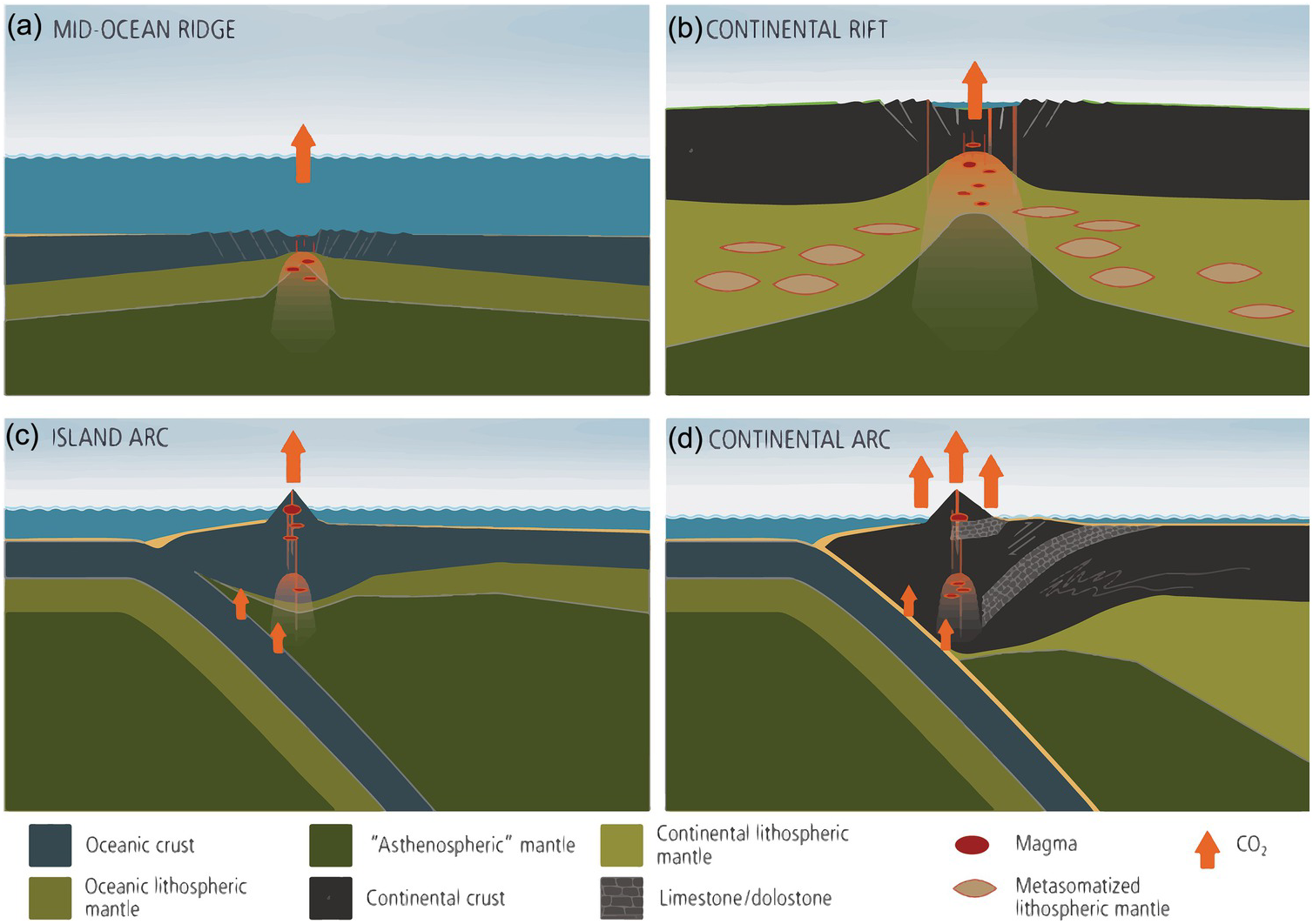
Global volcanic inputs of C are thus at least 0.54 Gton C/y if diffuse degassing estimates from Burton et al.Reference Burton, Sawyer and Granieri21 are considered. Global volcanic flux of C through geologic time, however, is likely to vary significantly due to variations in plume activity or global oceanic crust production rates.Reference Larson80, Reference Larson81 It has also been shown that continental arcs, because of magmatic interactions (via assimilation, melt-rock reaction, contact, and regional metamorphismReference Carter and Dasgupta82–Reference Carter and Dasgupta85) with ancient crustal carbonates stored in the continents emit significantly more CO2 than island arcs (Figure 11.10c and d); hence, the waxing and waning of continental arcs through time will also lead to increases in volcanic CO2 fluxing.Reference Lee22, Reference Lee and Lackey23, Reference Mason, Edmonds and Turchyn86–Reference McKenzie88 Enhanced continental rifting could also lead to enhanced CO2 production.Reference Lee79, Reference Johansson, Zahirovic and Muller89, Reference Brune, Williams and Muller90
11.4.1.2 Metamorphic Inputs
Metamorphic inputs of C involve thermal breakdown of crustal carbonates. The dominant decarbonation reactions occur by reaction of carbonate with silica:
to form calc-silicate minerals, such as wollastonite and other pyroxenes.Reference Ferry91, Reference Spear92 These reactions operate at temperatures (400–600°C) that can be achieved over large areas during regional metamorphism. The presence of water, which decreases CO2 activity, further decreases the temperatures needed for reaction (300°C).Reference Ague and Nicolescu93 Metamorphic decarbonation can thus be pervasive in subduction zones, continental collisions, or continental extension.
Estimates of metamorphic CO2 degassing rates, particularly on a global scale, are challenging to quantify because metamorphic degassing is diffuse and spatially heterogeneous. It has been shown that the metamorphic CO2 flux in the Himalayas may be large, being similar to or even higher than that removed by silicate weathering from the Himalayas themselves.Reference Evans, Derry and France-Lanord94 Kerrick and CaldeiraReference Kerrick and Caldeira20 have suggested that metamorphic outgassing associated with orogenies during the Eocene could be anywhere between 0.04 and 0.20 Gton C/y (Figure 11.8). Importantly, even though these numbers are highly uncertain, their magnitudes are potentially equal to or greater than that of MOR degassing.
11.4.1.3 Carbonate and Organic Carbon Weathering
Weathering of ancient crustal carbonates and organic C represents another large input of C into the exogenic system. Carbonate weathering involves the dissolution of the carbonate fraction in eroding material by the following reaction
For each mole of CO2 consumed, dissolution releases 2 moles of bicarbonate (HCO3–), resulting in a net contribution of 1 mole of CO2 to the ocean–atmosphere system. However, because carbonate dissolution introduces Ca2+ and Mg2+ ions as well as bicarbonate ion into the ocean (in silicate weathering, CO2 is consumed), precipitation of carbonate follows:
On timescales longer than ~10 ky, carbonate dissolution and precipitation balance, such that carbonate weathering is not thought to significantly influence the long-term evolution of exogenic C.Reference Berner3
Another source of CO2 is weathering of organic C, wherein a reduced form of C is oxidized by the atmosphere to form oxidized C; that is, CO2:
Weathering of “black” shales would be an example of oxidative weathering of organic C. Like carbonate weathering, oxidative weathering of organic C is assumed to be balanced on short timescales by organic C burial:
so that on long timescales, the net effect of organic C weathering on exogenic C is often assumed to be negligible.Reference Berner3 Such a close balance between organic C fluxes is presumably regulated by atmospheric O2 concentrations. For example, increases in the oxidative weathering of organic C would lead to lower atmospheric (and seawater) O2 concentrations, which are thought to enhance organic matter burial. However, there is still uncertainty as to whether the organic C cycle is in balance because many of the redox fluxes are not well constrained. A full treatment of organic C weathering must be coupled with the global oxygen cycle.Reference Berner3, Reference Lee95
Although weathering of carbonates and organic C are likely balanced on timescales >100 ky, it is nevertheless important to appreciate their magnitudes (Figure 11.8). The oxidative weathering rate of organic C is thought to be ~0.05 Gton C/y,Reference Petsch25 and global compilations and river chemistry indicate a modern carbonate weathering flux of 0.148 Gton C/y (these calculations assume stoichiometric weathering).Reference Gaillardet, Dupre, Louvat and Allegre17 Together, these fluxes are comparable to the total volcanic flux of CO2 today. To illustrate the magnitude of the carbonate weathering flux, it is now established that the alkalinity in global rivers is dominated by carbonate weathering rather than silicate weatheringReference Gaillardet, Dupre, Louvat and Allegre17, Reference Evans, Derry and France-Lanord96, Reference Jacobson, Blum and Walter97 due to the fast dissolution kinetics of carbonates compared to silicates. Because these weathering fluxes are large, any imbalances in weathering of carbonates and organic C versus carbonates and organic C burial could lead to large swings in exogenic C on short timescales.Reference Walker and Opdyke98 The magnitudes and timescales of such swings are ultimately limited by the fact that ocean chemistry adjusts to maintain a relatively constant saturation state with respect to calcium carbonate phases.Reference Zeebe and Westbroek99 Estimates of the response timescale of carbonate buffering in the ocean are around 6000 years.Reference Zeebe and Westbroek99 Such weathering probably cannot be truly ignored even on >100‑ky timescales, especially if the ratio of organic C to carbonate weathering (or deposition) varies with time or if the distribution of carbonate and organic C deposition changes with time (deep sea versus continental shelves). Finally, it has recently been shown that oxidative sulfide weathering in organic-rich sedimentary rocks can lead to a net release of CO2 if the resulting sulfuric acid reacts with nearby carbonates.Reference Torres, West and Li100 Unlike carbonate (by carbonic acid) or organic C weathering, sulfide weathering can serve as a long-term input of CO2 if there is an imbalance in the S cycle.
11.4.1.4 Carbon Inputs Internal to the Exogenic System
Geologic inputs (volcanic and weathering) of CO2 into the exogenic system are small compared to fluxes internal to the exogenic system. For context, exchange between the terrestrial biosphere and atmosphere is ~60 Gton C/y and between the surface ocean and atmosphere is ~70 Gton C/y.Reference Sundquist and Visser11 Present anthropogenic CO2 emissions from fossil fuels and cement production is ~10 Gton C/y,Reference Friedlingstein26 which exceeds volcanic emissions by more than 50 times. These large fluxes are likely not important on long timescales as they operate on much faster timescales within the exogenic system. Nevertheless, on short timescales, any imbalances in the system associated with these fluxes or sources can lead to large, short-lived excursions in atmospheric CO2. Intriguingly, terrestrial biomarkers present in river sediments yield apparent radiocarbon “ages” in excess of 1000 years,Reference Galy and Eglinton101 which implies that imbalances between terrestrial photosynthesis and respiration may play a role in the exogenic C cycle over millennial timescales.
11.4.2 Carbon Outputs
11.4.2.1 Silicate Weathering Chemistry and Carbonate Precipitation
While all silicate minerals undergo dissolution, Ca- and Mg-bearing silicate minerals in the continental crust (e.g. hornblende, plagioclase, pyroxene, and, to a lesser extent, olivine and biotite for Mg only) are often considered the most important in the context of the long-term global C cycle because the dissolved Ca2+ and Mg2+, after traveling to the ocean via rivers, eventually precipitate to form calcium and magnesium carbonates in the marine environment. However, alkalinity supplied by the dissolution of Na- and K-bearing silicates dominates the silicate-derived riverine flux and contributes to CaCO3 precipitation via ion-exchange reactions. Additionally, some portion of the Na and K flux is thought to react with Si and Al to form clay minerals in a process termed “reverse” weathering, which, by modifying the seawater alkalinity balance, contributes CO2 back into the atmosphere.Reference Isson and Planavsky102
The dominant Ca-bearing mineral in the average continental crust is plagioclase, but for simplicity, silicate weathering of calc-silicates is often idealized by lumping all calc-silicates into the form of wollastonite, CaSiO3 (however, wollastonite is exceedingly rare in the continental crust!). The sequence of reactions begins with formation of carbonic acid by equilibration with CO2 in the atmosphere or subsurface pore-space:
This is followed by release of H+ ions:
which react with calc-silicates to release Ca2+ and Si4+ in the form of silica hydroxides into river waters (an identical reaction can be written for MgSiO3):
CaReference Walker, Hays and Kasting2+ ions combine with the major carbonate species in seawater, bicarbonate (HCO3–), to precipitate calcium carbonate in the marine or lacustrine environments (and dissolved silica precipitates as chert, SiO2):
If we combine the above equations, we arrive at the commonly cited net reaction for calc-silicate weathering:
The equivalent reaction for plagioclase is:
Dissolution of calc-silicates followed by precipitation of carbonates results in net consumption of CO2. Estimates of the terrestrial silicate weathering output of C in the form of carbonate are typically drawn from the dissolved flux of cations in river waters, assuming that most of the Ca and Mg ions and some portion of the Na and K fluxes (via exchange) eventually precipitate as Ca–Mg carbonates. Modern carbonate burial fluxes associated with silicate weathering only are thought to be between 0.13 and 0.38 Gton C/y (Figure 11.8).Reference Sundquist and Visser11 As discussed above, a fraction of the Ca ion flux in rivers comes from dissolution of carbonate, so the carbonate fraction must be subtracted. According to Gaillardet et al.,Reference Gaillardet, Dupre, Louvat and Allegre17 the global terrestrial carbonate-corrected silicate weathering flux may be on the low end of the above range, at ~0.14 Gton C/y. Newer estimates from Moon et al.Reference Moon, Chamberlain and Hilley103 revise the silicate weathering flux to even lower values (0.09 ± 0.02 Gton C/y), but completely exclude Na and K from these calculations.
Not accounted for in the above estimates of the silicate weathering–carbonate precipitation flux is the role of seafloor basalt alteration. A number of studies have shown that the CO2 content of altered oceanic crust can be quite high. For example, Mesozoic-aged altered oceanic crust can contain up to 2.5 wt.% CO2, compared to ~0.5 wt.% CO2 in late Cenozoic oceanic crust.Reference Coogan and Gillis104–Reference Staudigel, Hart, Schmincke and Smith107 These studies estimate that C sequestration via seafloor alteration could amount to 0.006–0.036 Gton C/y,Reference Coogan and Gillis104, Reference Staudigel, Hart, Schmincke and Smith107, Reference Coogan and Dosso108 similar to modern inputs of C via MORs, but less than the terrestrial silicate weathering sink (Figure 11.8).
11.4.2.2 Photosynthesis and Organic Carbon Burial
Most of the C in the atmosphere–ocean system today is in an oxidized form. A fraction of this C is reduced through autotrophic organisms by oxygenic photosynthesis to form organic C (other types of photosynthesis could have dominated early in Earth’s history):
Here, organic C is approximated as “CH2O” and differs from CO2 in being composed of reduced C (C3+ or less) as compared to oxidized C in CO2 (C4+). Much of the organic C is respired (oxidized) back to the atmosphere through organic C decomposition or indirectly through consumption by heterotrophic life, reversing the above reaction. In net, photosynthetic production and oxidative destruction of organic C are roughly in balance, even on timescales as short as years or even days in some cases. However, a small fraction of organic C “leaks” out from the exogenic system through sedimentary burial. This burial of organic C, like the burial of carbonate, represents a net long-term sink of C from the exogenic system, but differs from the carbonate cycle in that burial of organic C also generates free O2, with implications for atmospheric oxygenation. Buried at great enough depths, organic C becomes part of the crustal reservoir in the form of “fossil” C.
Estimates of the organic C burial rate are typically inferred from the C isotopic composition of seawater. Carbon isotopes are fractionated to light values during photosynthesis but are not strongly fractionated during carbonate precipitation (due to a lack of redox change). Assuming the isotopic compositions of long-term C inputs into the exogenic system are mantle-like, the fraction of organic C (commonly referred to as forg in the literature) buried can be estimated from the C isotopic composition of seawater or marine carbonates. Except for short-term excursions, the 13C/12C of seawater has remained relatively constant at 4–5 per mil higher than the mantle for most of Earth’s history, which translates into an organic C burial fraction of ~20–25% relative to total C burial (carbonate + organic C).Reference Berner3, Reference Berner9, Reference Schidlowski109
Whether forg has indeed remained constant and, if so, why, remain important questions.Reference Krissansen-Totton, Buick and Catling110 It may be worth exploring whether the isotopic offset between inorganic and organic C remains constant through Earth’s history. There is also the possibility that the weathering of carbonates or the metamorphic outgassing efficiencies of crustal carbonates and organic C are different enough that the isotopic composition of the long-term inputs of C into the exogenic system need not balance with mantle-like values at all times.Reference Lee22, Reference Mason, Edmonds and Turchyn86, Reference Shields and Mills111
11.4.2.3 Subduction Flux
Subduction of the oceanic lithosphere and accompanying marine sediments is the primary mechanism by which C is “permanently” removed from Earth’s surface and recycled back into the endogenic system. Subduction itself is not a direct negative feedback in the climate system because it only serves to transport already sequestered C into the mantle. Subduction plays an indirect role in the longer-term exogenic C cycle and climate if it contributes some of its C to arc magmas or it influences the efficiency of C released from the sub-arc mantle wedge and into arc magmas.
Based on estimates of the carbonate and organic C distribution of marine sediments and the amount of C in seafloor altered crust (mostly in the form of carbonate),Reference Coogan and Gillis104, Reference Alt and Teagle105, Reference Staudigel, Hart, Schmincke and Smith107, Reference Plank and Langmuir112 Dasgupta and HirschmannReference Dasgupta and Hirschmann18 estimated a modern global subduction flux of 0.024–0.048 Gton C/y (Figure 11.8). This is comparable to the lower end of estimates of global magmatic degassing. How much of this subducted C is released back into the crust or atmosphere through volcanism and how much continues deep down into the mantle is debated. Because the temperature needed for decarbonation reactions increases with pressure, the subducting slab needs to heat up sufficiently for efficient decarbonation.Reference Kerrick and Connolly113, Reference Kerrick and Connolly114 In the absence water, slab decarbonation (either during subsolidus conditions or during partial melting) is not expected to be efficient in most modern subduction zones, except for perhaps the youngest and hottest ones.Reference Dasgupta51, Reference Kerrick and Connolly114 Slab decarbonation would have been more efficient in the Archean if the thermal states of these ancient subduction zones were higher than today.Reference Dasgupta51 In the presence of water, CO2 activities decrease, depressing reaction temperatures.Reference Spear92 Thus, dehydration of serpentine in the slab could give rise to “water-fluxed” decarbonation or carbonate dissolution, enhancing the efficiency of decarbonation (see Refs. Reference Kelemen and Manning49 and Reference Ague and Nicolescu93). Small amounts of C in the form of graphitized organic C in slabs are still expected to survive fluid-fluxed melting (e.g. Ref. Reference Duncan and Dasgupta50). In any case, release from the slab does not guarantee that such C quantitatively returns to the exogenic system through arc volcanoes.
11.5 Efficiency of the Silicate Weathering Feedback
In this section, we discuss the kinetics of silicate weathering (we ignore organic C burial because it is a smaller flux). The kinetics of silicate dissolution are much slower than those of carbonate precipitation in the oceans. The ocean is oversaturated in carbonate and therefore any Ca that enters the ocean tends to precipitate on short timescales. Thus, silicate dissolution is the rate-limiting step. The rate (moles/y) of dissolution should scale asReference Kump, Brantley and Arthur115, Reference Winnick and Maher116:
where k is a kinetic rate constant (moles/m2/y) defined relative to a specified surface area A (e.g. geometric or total surface area) and represents a measure of the efficiency of dissolution, aH+ is the activity of hydronium ions in solution, and n represents the order of the chemical reaction. Hydronium ion activity aH+ depends on the pCO2 in equilibrium with weathering fluids:
 (11.23)
This relation with pCO2 is one potential source of a negative feedback in the global C cycle. If the pCO2 of weathering fluids increases as the pCO2 of the atmosphere increases (e.g. via changes in primary productivityReference Pagani, Caldeira, Berner and Beerling117), silicate dissolution rates increase, which results in more rapid removal of CO2 from the atmosphere through carbonate precipitation. In the Earth system, the global silicate weathering feedback must also include the effects of atmospheric CO2 on the hydrologic cycle, vegetation, and so forth, so (11.23) is only meant to conceptually represent the most elementary level of CO2 feedback.
Increases in pCO2 should also lead to increases in temperature due to the greenhouse effect (~2.4–4.8°C per doubling of pCO2118). The negative feedback is enhanced because of the temperature dependence of the kinetics of dissolutionReference Laidler119; that is:
where ko is a pre-exponent constant that depends on the type of mineral, EA is the activation energy for dissolution, R is the gas constant, and T is temperature. If pCO2 increases, temperature increases, which in turn increases dissolution rates, thereby increasing rates of CO2 drawdown by silicate weathering (followed by carbonate precipitation).
As we scale up from the mineral to the global scale, additional influences on weathering rate must be considered. For example, if chemical weathering reactions occur close to thermodynamic equilibrium, weathering fluxes will scale with the total water flux through the system.Reference Maher and Chamberlain120 Chemical weathering can also be enhanced by biology, through bioturbation and higher subsurface pCO2 levels. Because hydrology and biology can both accelerate chemical weathering, these processes can act as negative feedbacks if increases in global temperature, perhaps driven by increases in atmospheric CO2, accelerate the hydrologic cycle.Reference Maher and Chamberlain120, Reference Held and Soden121 Finally, chemical weathering can also be limited by the rate at which fresh rock is supplied by physical weathering and erosion. Erosion can behave as a negative feedback under conditions in which erosion is accelerated by higher hydrologic or biological activity. Under conditions in which erosion is largely controlled by tectonics, which do not depend on climate, the feedback would be poor.
Combining all of these factors results in a complicated functional form of the silicate weathering feedback. BernerReference Berner122 proposed the following generalized empirical equation:
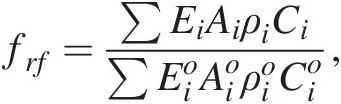
where FSi′ represents the silicate weathering flux contributing to carbonate precipitation, fw is the function describing the sensitivity of mineral dissolution to pCO2, frf represents mean global relief, fpl represents the effect of plants, and fro represents average water runoff, with all functions normalized to present conditions. In the Berner model, the temperature effect is subsumed into the effect of temperature on runoff and the effect of pCO2 on chemical weathering. For the purposes of this chapter, the exact functional relationships are not critical (see Ref. Reference West123). These relationships must be calibrated against field studies to be relevant for a particular region or a given time period in Earth’s history.
If we consider fw, fpl, and fro to all be related to pCO2 through a series of transfer functions, we can combine them into one master function fw*, which describes the dependency of weathering on pCO2:
 (11.26)
This leaves the relief term in Berner’s model, frf, as the only function independent of pCO2. The relief term is fundamental as it relates to erosion rate. Erosion supplies fresh rock to the surface so that it can undergo chemical weathering. At low erosion rates, soil mantles, although chemically depleted due to their long residence times in the weathering regime, no longer contain weatherable minerals. On long timescales, what ultimately drives erosion is topography, which itself is driven by tectonism or magmatism.
We can describe frf as the weighted average flux of fresh rock supplied by erosion relative to the global mean today:
 (11.27)
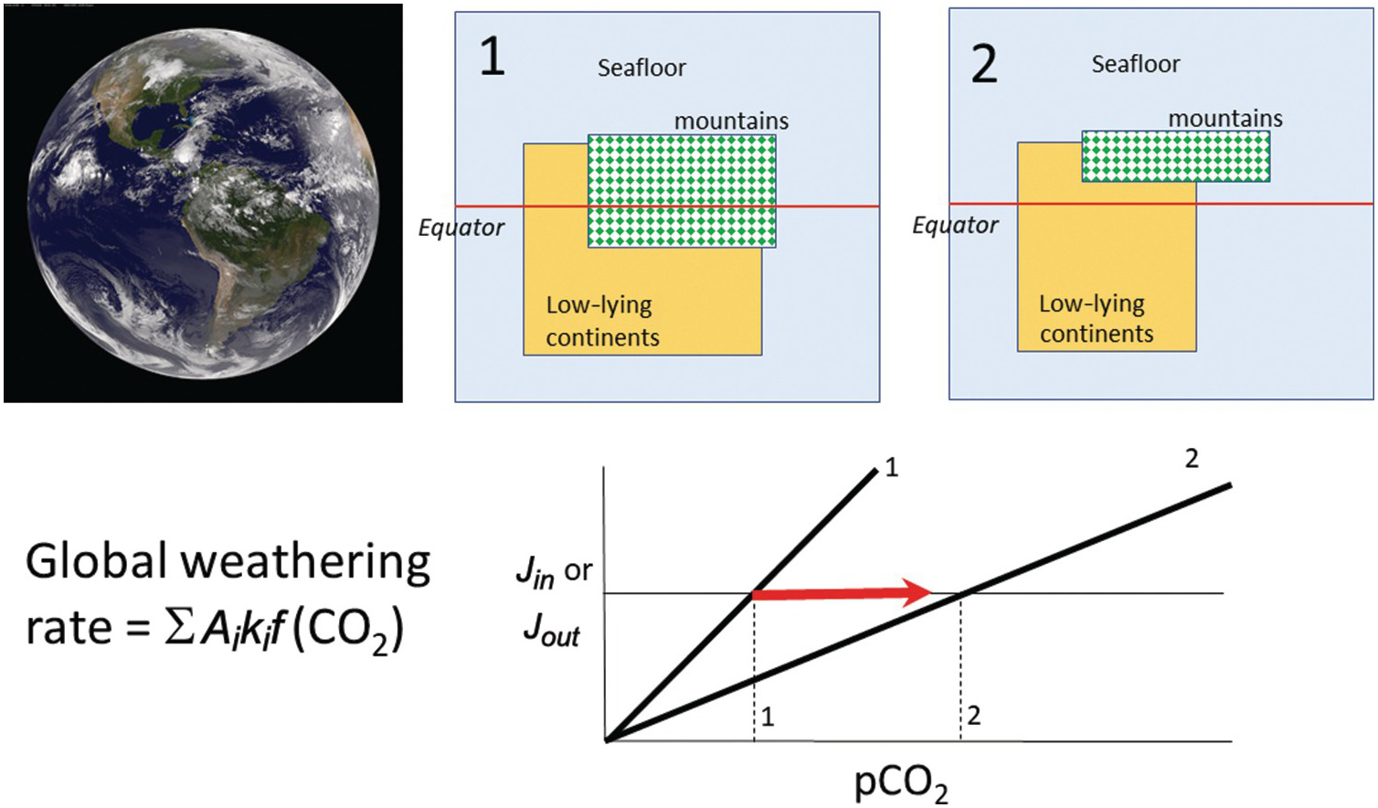
where Ei is the erosion rate (m/y) in a given region i and Ai is the map area of region i, with the quantities in the denominator representing present-day conditions (Figure 11.11). The summation signs denote summation over the entire continental area. What is important is that the area of orogenic activity on Earth is not constant. For example, the hypothesis that mid-Cenozoic cooling was triggered by enhanced erosion associated with the Himalayan orogeny is based on the premise that the mean area of orogenies and mean erosion rates increased.Reference Raymo, Ruddiman and Froelich124, Reference Raymo and Ruddiman125 A simple way to understand the effect of increased orogenic belts is to consider the case in which the silicate weathering response to changes in pCO2 is linear. In such a scenario, doubling the length of orogenic belts (i.e. doubling the mass of silicate minerals exposed at the surface per unit time) would increase the sensitivity (e.g. the slope on the silicate weathering-driven burial rate of carbonate versus pCO2) of the global silicate weathering feedback by a factor of 2 (Figure 11.11). If long-term inputs of CO2 into the exogenic system do not change, exogenic CO2 would decrease by a factor of 2, cooling the atmosphere. This simple exercise also implies that in a world devoid of orogenic belts, such as in the extreme case of flat continents riding near sea level, the strength of the negative silicate weathering feedback would be substantially decreased.
The global silicate weathering rate can be described by partitioning Earth into different types of weathering sites, each defined by different weathering kinetics (e.g. seafloor, orogens, and low-relief continents). Changes in the proportions of low-relief continents or orogenic belts will change the global sensitivity of the weathering feedback. A decrease in area of continents and orogens results in a decrease in the weathering feedback strength (states 1 to 2), leading to an increase in pCO2 (states 1 to 2).
Finally, temporal changes in the composition of the bedrock undergoing weathering can be important. It is widely agreed that the average composition of the continental crust is intermediate in composition, equivalent to the composition of a typical andesite.Reference Rudnick and Fountain126 These published averages often obscure the fact that the continental crust is highly heterogeneous, containing rocks of all types, from ultramafic rocks (serpentinites and peridotites) to mafic rocks (basalts) to highly silicic rocks (e.g. rhyolites). Because different lithologies weather at different rates, have different temperature sensitivities, and supply major cations in different proportions, the composition of rocks within an active orogeny matters. For example, the CaO content of a typical basalt/gabbro is between 10 and 15 wt.%, that of andesite/granodiorite is between 6 and 8 wt.%, and that of a rhyolite/granite is less than 3 wt.%. Additionally, available estimates suggest that basalts weather, on average, approximately two times faster than granitic rocks, but this ratio varies as a function of climatic conditions.Reference Ibarra127 This compositional effect can be incorporated through the erosional term, frf:
 (11.28)
where Ci represents the concentration of Ca and Mg (note that not all Mg is sequestered as carbonate) and ρi is rock density. Equation (11.28) describes the availability of Ca and Mg due to differences in composition. Depending on the composition of the crust undergoing orogeny, the sensitivity of the regional chemical weathering feedback could vary by a factor of 3–5 due to the availability of Ca and Mg (there is also a small effect of Na and K exchange with Ca in the ocean). Added to this compositional effect will also be the faster dissolution kinetics of basalt versus granite,Reference Gaillardet, Dupre, Louvat and Allegre17, Reference Ibarra127–Reference Gislason, Arnorsson and Armannsson129 which would modify ki in (11.22). A number of studies have shown that the composition of orogenies can vary depending on orogenic style or geologic history.Reference Farner and Lee130 There may have also been Gy-scale changes in the composition of magmatism, from mafic to a felsic crust around 2.5 Ga,Reference Lee95, Reference Tang, Chen and Rudnick131, Reference Keller and Schoene132 suggesting that the weathering feedback strength could have fundamentally changed over Earth’s history.
In summary, silicate weathering represents a negative feedback in the whole-Earth C system because of the dependency of weathering on pCO2 through direct and indirect effects on temperature, biological activity, and precipitation/runoff. One of the most important controls of the strength of the feedback is the area of orogenic belts, where chemical weathering is facilitated by high erosion rates. Large fluctuations in the intensity and distribution of orogenic activity could play a key role in modulating the strength of the silicate weathering feedback.
11.5.1 Seafloor Weathering Feedback
In Section 11.4.2, we showed that carbonate sequestration via seafloor alteration was comparable to the CO2 flux out of MORs, begging the question of how important seafloor alteration is as a negative feedback. Coogan and DossoReference Coogan and Dosso108 inferred that the activation energy for rock dissolution during seafloor alteration is ~92 kJ/mol, similar to that for the dissolution of various silicate minerals under conditions relevant for terrestrial weathering.Reference Kump, Brantley and Arthur115 If direct temperature effects alone were the dominant control on the negative weathering feedback, one would expect the strength of the seafloor alteration feedback to be equivalent to that of the terrestrial feedback, all other variables being equal. However, as discussed above, many other processes operate. In the case of terrestrial weathering, the effects of runoff on erosion will amplify the strength of the negative feedback. In the case of seafloor alteration, there are no erosional mechanisms that replenish fresh rock for dissolution, so the weathering system would be closer to equilibrium and the kinetics of weathering would be slow. These factors could reduce the net sensitivity of seafloor weathering to global temperature. A recent inverse study of the paleoclimate record suggested that seafloor weathering was not as important as continental weathering over the last 100 My.Reference Krissansen-Totton and Catling133 However, during periods of low orogenic activity, the proportional contribution of the seafloor to the global feedback indeed increases (Figure 11.11). For example, silicate weathering could have been dominated by seafloor weathering in the Archean if most of the continents were below sea level.Reference Lee134 In such a case, the strength of the seafloor weathering feedback becomes critically important to understand.
11.6 Discussion
11.6.1 Framework for Modeling Whole-Earth C Cycling
Earth systems modeling is traditionally rendered in terms of boxes with estimates of reservoir sizes and fluxes (Figure 11.3 and Sections 11.3 and 11.4). However, in such renditions, fluxes and reservoir sizes are snapshots in time and cannot be applied back in time if reservoir sizes change. Instead of using fluxes, it is better to use the kinetics of C transfer between reservoirs, as kinetic rate “constants” do not depend on reservoir size even if the system is not at steady state. Rate constants can of course change if the fundamental physics and chemistry change. If the rate constants are known, (11.1) can be expressed as follows for a linear system:
 (11.29)
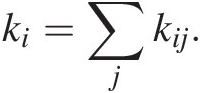
where kij represents the rate constant describing the transfer of C from reservoir i to j. The first term represents inputs into reservoir j from all reservoirs i. The second term represents outputs from reservoir i into different reservoirs j. Solving (11.29) for a system of interacting reservoirs involves solving a system of equations using a multidimensional (i × j) matrix kij, which can be estimated from modern fluxes if the system is near steady state. We can divide the flux associated with any given process by the size of the reservoir from which C is removed, resulting in a fractional rate constant. The sum of all rate constants describing removal of C from a reservoir i is the total rate constant, ki; that is:
 (11.30)
The inverse of the total rate constant represents the residence time τi of C in reservoir i from which C is extractedReference Lee, Lee and Wu135:
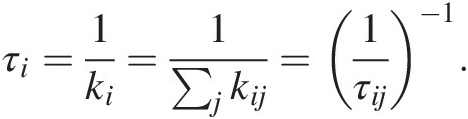 (11.31)
In Figure 11.12, we present reservoir residence times (leftmost column) and the rate constant matrix, the latter represented in the form of fractional response times 1/kij, which are more intuitive than fractional rate constants. In Figure 11.12, the row denotes the reservoir (i) from which C is being removed and the column denotes the reservoir (j) receiving C from i. Estimates of exogenic rate constants were guided by modern fluxes and reservoir sizes from Table 11.2 and an assumption of near steady state. For endogenic reservoirs, which are larger and may not be at steady state, our estimated rate constants are speculative. The modeler is encouraged to modify the endogenic rate constants to explore the behavior of the system. Empty boxes indicate the absence of flux. Boxes with a question mark indicate that there is a flux, but the magnitude of the flux and the rate constant are poorly known or change considerably with time. For example, degassing of the deep ocean to the atmosphere varies considerably between glacial–interglacial cycles. Transfer of C between the upper mantle and lower mantle is uncertain because it depends on the flux of mantle material between the two reservoirs, which is not known.
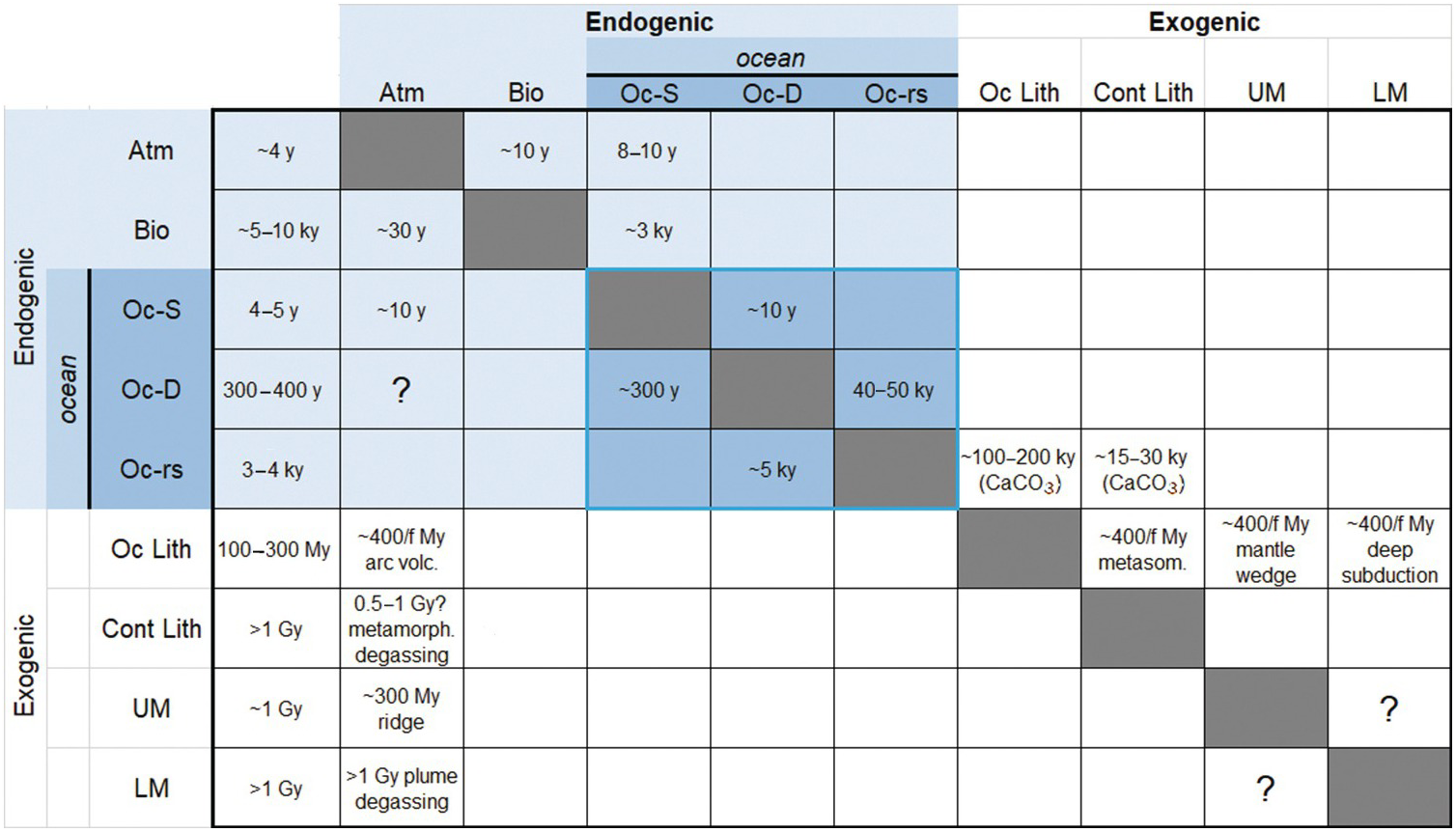
Matrix of kinetic rate constants between reservoirs, expressed as fractional response times or the inverse of the kinetic rate constant (τij = kij–1). Each cell corresponds to the transfer of C from reservoir i to j, where i correspond to the row and j corresponds to the column. Empty or gray cells indicate a lack of C transfer from i to j. Cells with a question mark indicate that C transfer occurs, but the magnitude and rate constant are not known or vary significantly in time; these are left for the reader to vary in their own studies. Blue-shaded cells represent exogenic reservoirs. The blue-outlined group of cells represents ocean reservoirs, including reactive marine sediments. The leftmost column shows residence time τi of reservoir i. Reservoir symbols as follows: Atm = atmosphere; Bio = terrestrial biosphere; Oc-S = surface ocean; Oc-D = intermediate and deep ocean; Oc-rs = reactive marine sediment; Oc Lith = oceanic lithosphere, which includes oceanic crust and oceanic lithospheric mantle; Cont Lith = continental lithosphere, which includes continental crust (sediments + basement) and CLM; UM = upper mantle (<670 km); LM = lower mantle (>670 km). Earth’s core is excluded. “f” corresponds to the fraction of C from the subducting oceanic lithosphere that is lost to a particular reservoir.
11.6.2 Is Earth’s Mantle Degassing or “Ingassing”?
A key question is whether mantle degassing rates are balanced by recycling of C back into the mantle through subduction. The only direct way to answer this question is to compare mantle degassing fluxes to subduction fluxes, but these quantities are uncertain. A better approach is to explore possibilities through a forward box modeling approach as discussed in Section 11.6.1 and depicted in Figure 11.12. Rate constants can be allowed to vary with time as constrained by the physical evolution of Earth following simple, parameterized convectionReference McGovern and Schubert136 rather than full-scale coupling of thermodynamic and geodynamic models. For example, it is relatively straightforward to develop petrologically constrained scalings for mantle and crustal degassing as a function of mantle thermal state and convective vigor, with the goal of quantifying degassing at MORs, subducting slabs, arcs, and intraplate environments. Important quantities would be the kinetics of chemical weathering, but also where carbonates are deposited. In the extreme scenario in which all carbonates are deposited on continental shelves, which do not subduct, then there is little recycling of C back into the mantle. As far as we know, there is not yet any whole-Earth box model that has incorporated the nature of how C is deposited (oceans versus continents). The important controls of where carbonates are deposited will be total area of shallow continental margins, the evolution of life, and the chemistry of the oceans.Reference Ridgwell and Zeebe137, Reference Ridgwell138 Variations of continental shelf area with time could be one of the most important factors controlling the rate at which C accumulates at the surface, as there are times in Earth’s history when continents may have been wholly submerged,Reference Lee134, Reference Korenaga, Planavsky and Evans139, Reference Flament, Coltice and Rey140 with most C being deposited in epicontinental seas, leaving little to be deposited in the deep sea for subduction.
In any case, we know that sedimentary rocks have accumulated on the continents over Earth’s history. We also know that other incompatible elements, such as U, Th, and K, among others, have progressively migrated into the continental crust, leaving behind a depleted upper mantle. If C behaves incompatibly, then the continental crust and CLM C budget have likely grown with time as well. This growing continental reservoir of C serves as a capacitor, which can enhance outgassing rates by metamorphic or magmatically driven decarbonation of the lithosphere in continental arcsReference Lee22 or continental rifts.Reference Lee79 If direct mantle degassing rates have not changed with time, total outgassing rates from the endogenic system should have increased with time. Alternatively, if mantle degassing rates are thought to have decreased significantly through time, lithospheric amplification could have partly compensated for this decline. Understanding how total outgassing rates from Earth’s interior have changed through time will have profound implications for the evolution of other volatiles, whose chemistries may be linked to C. For example, an increasing outgassing flux of C would result in increased photosynthetic production of atmospheric oxygen.Reference Lee95
11.6.3 What Drives Greenhouse and Icehouse Conditions?
On 10–100‑My timescales, Earth’s climate fluctuates between greenhouse and icehouse states, the latter being characterized by permanent polar ice sheets and the former without permanent polar ice. For example, the late Jurassic to the early Cenozoic was characterized by greenhouse conditions, where temperatures were thought to be >10°C higher than today and any ice sheets were thought to be ephemeral. This greenhouse interval was punctuated by a number of short-term (<100‑ky) excursions to even warmer conditions, often referred to as “hothouse” events.Reference Jenkyns, Forster, Schouten and Sinninghe Damste141
Earth began to cool around 50 Ma in the mid-Cenozoic based on the seawater oxygen isotope record, with southern hemisphere glaciation (Antarctica) beginning ~35 Ma, followed by the development of the northern hemisphere ice sheet ~5 Ma.Reference Zachos, Dickens and Zeebe4, Reference Zachos, Pagani, Sloan, Thomas and Billups36 Earth in the last several million years has been characterized by bipolar glaciation, and because of the albedo effect of ice, subtle variations in solar insolation driven by orbital dynamics can drive short-term cycles (10–100 ky) of ice sheet growth and retreat. Thus, superimposed on the late Cenozoic icehouse baseline are geologically rapid periodic fluctuations of temperature, ice volume, and eustatic sea level tuned to orbital dynamics. During greenhouse intervals, apparent changes in relative sea level (e.g. sequence boundariesReference Haq, Hardenbol and Vail142, Reference Vail, Mitchum and Thompson143) recorded during greenhouse conditions most likely have origins that are different from glacioeustasy, such as external changes in sediment supply. While rapid fluctuations in sea level are a defining characteristic of an icehouse world, short-lived hothouse excursions – a characteristic feature of greenhouse intervals – appear to be absent from icehouse worlds.
Two questions follow. First, what controls baseline climate? Second, what conditions allow for and trigger short-term excursions to extreme warm and cold climates? In general, baseline climate on >10‑My timescales is ultimately controlled by the amount of greenhouse gases in the atmosphere, namely CO2 for most of Earth’s history. Orbital dynamics are too rapid, while changes in the sun’s luminosity only explain changes over Gy. Understanding long-term baselines comes down to understanding what controls the steady state. The combination of volcanic/metamorphic forcings (input) and the efficiency of the silicate weathering feedback defines a given steady state, and it is the variations in these two quantities that we seek to understand.Reference Caves, Jost, Lau and Maher30
11.6.3.1 Greenhouse Intervals
A widely held view is that the late Mesozoic and early Cenozoic greenhouse conditions were driven by a 1.5- to 2-fold increase in MOR spreading rates, leading to an increase in CO2 output from the mantle.Reference Berner3, Reference Larson80, Reference Larson81 The contribution from oceanic spreading may have been enhanced by a greater emplacement frequency of large igneous provinces.Reference Larson80 Mid-Cenozoic cooling toward icehouse conditions is widely thought to have been driven by an increase in the efficiency of the silicate weathering feedback through the collision of India with Eurasia and the uplift of the Himalayas and Tibet.Reference Raymo, Ruddiman and Froelich124, Reference Raymo and Ruddiman125
There are, however, reasons to explore other hypotheses. One question is whether enhanced MOR spreading was able to sustain a Cretaceous pCO2 that was 5–10 times higher than present (Figure 11.1b). If CO2 concentrations in Mesozoic MORBs were similar to today’s, the increase in CO2 production rates would scale roughly linearly with the increase in spreading rate. Assuming a linear negative feedback, the enhanced spreading rates would lead to only a 1.5- to 2-fold increase in atmospheric CO2, or the global silicate weathering feedback would have to have been less efficient. The latter seems unlikely because weathering kinetics should increase in the hotter and wetter conditions of greenhouse climates. Furthermore, the late Mesozoic to early Cenozoic was characterized by significant orogenic activity in the form of Andean-style continental arcs. Thus, weathering feedback strength during the late Mesozoic greenhouse should have been high, requiring even higher inputs of CO2 to sustain the elevated pCO2.
Recently, it has been suggested that length of continental arcs during the Cretaceous was 1.5–2 times longer than that of the mid-Cenozoic.Reference Lee22 Due to the large amounts of carbonate stored in the continental crust, continental arcs may degas more CO2 through metamorphic and magmatically induced decarbonation of crustal carbonate; thus, a global chain of continental arcs might amplify global CO2 outgassing.Reference Lee22, Reference Mason, Edmonds and Turchyn86, Reference Aiuppa, Fischer, Plank, Robidoux and Di Napoli144 Long-term fluctuations in the length of continental arcs, driven by the assembly and dispersal of continents, have been suggested to drive greenhouse–icehouse oscillations based on studies of the detrital zircon record and arc length through time.Reference McKenzie88, Reference Cao, Lee and Lackey145 Lee et al.Reference Lee22 showed that the long Cretaceous continental arcs may have supported a flux of 0.09–0.13 Gton C/y, more than twice that of global magmatic arcs today (Figure 11.8b). This hypothesis has been contested by Pall et al.,Reference Pall146 who argue for a weak correlation between carbonate-intersecting continental arcs and high pCO2. However, this study did not incorporate the Precambrian distribution of carbonates or uncertainties in the paleo-pCO2 record. In any case, other factors to be considered are the competing effects of enhanced erosion and weathering during continental arc magmatismReference Jiang and Lee147, Reference Lee, Thurner, Paterson and Cao148 and the slab contribution to CO2 fluxing through arcs, the latter requiring an understanding of slab composition, slab thermal state, and CO2 solubility in fluids and melts, among other factors. In any case, faster spreading, faster subduction, more plumes, and a transition to continental arcs over island arcs may operate together,Reference Lenardic149 making it difficult to ascribe greenhouse intervals to a single process.
11.6.3.2 Icehouse Drivers
Are long-lived icehouses driven by enhanced silicate weathering feedbacks or decreased outgassing from Earth’s interior? The Cretaceous greenhouse and mid-Cenozoic to present icehouse represent an ideal case study. It is widely thought that the Himalayan orogeny played a strong role in Cenozoic cooling beginning ~50 Ma by enhancing the silicate weathering feedback through enhanced erosion rates.Reference Raymo and Ruddiman125 However, the rise in 87Sr/86Sr often touted as an indicator of terrestrial weathering occurs ~38 Ma, well after cooling initiated.Reference Kent and Muttoni150, Reference Hodell151 Furthermore, radiogenic isotopes do not necessarily correlate with silicate weathering fluxes because source age and composition can be just as important.Reference Bataille, Willis, Yang and Liu152 For example, local weathering of ultramafics or black shales has an outsized influence on seawater 187Os/188Os.Reference Peucker-Ehrenbrink, Ravizza and Hofmann153, Reference Peucker-Ehrenbrink and Ravizza154 Similarly, weathering of carbonates or the very ancient basement influences 87Sr/86Sr.Reference Bataille, Willis, Yang and Liu152
These complications in interpreting seawater Sr isotopes raise a number of important questions. Is the Himalayan orogeny, in a regional sense, a net producer or consumer of CO2?Reference Evans, Derry and France-Lanord94, Reference Evans, Derry and France-Lanord96, Reference Jacobson, Blum and Walter97 This, combined with the possibility that regional metamorphism causes metamorphic decarbonation of crustal carbonates, should encourage vigorous discussion on the role of the Himalayan orogeny on global cooling. Recent studies have suggested that the closing of the Tethys ocean, which culminated in a transcontinental orogenic belt, of which the Himalayas are but one segment, involved the obduction of numerous island arc terranes and ophiolites, increasing global silicate weathering efficiency.Reference Jagoutz, Macdonald and Royden155 In an alternative scenario, Kent et al.Reference Kent156 suggested that the ~65‑Ma Deccan flood basalts in India may have increased global weathering efficiency as India migrated north into wet equatorial latitudes in the Cenozoic.
There is also the possibility that cool climates simply represent a decline in magmatic outgassing.Reference Berner, Lasaga and Garrels157 Evidence from detrital zircons and arc reconstructions have been used to suggest that long icehouse intervals coincide with periods of reduced continental arc activity, just as greenhouses have been suggested to correlate with enhanced continental arc activity.Reference Lee22, Reference McKenzie, Hughes, Gill and Myrow87, Reference McKenzie88, Reference Cao, Lee and Lackey145 The rise and fall of continental arcs offer an intriguing process for modulating the exogenic C system. When continental arcs are magmatically active, they are likely to be net producers of CO2, but after magmatism wanes, the remnant topography transforms continental arcs into regional sinks of CO2, resulting in a global increase in the efficiency of silicate weathering.Reference Jiang and Lee147, Reference Lee, Thurner, Paterson and Cao148 In such a scenario, magmatic outgassing drives greenhouse intervals, which are followed by icehouse intervals when the same orogens die magmatically but continue to weather (Figure 11.13).
(a) Case study of a magmatic orogen: Cretaceous Peninsular Ranges batholith in southern California, USA.Reference Jiang and Lee147 Red line shows the observed magmatic production rate and symbols with error bars represent inferred erosion rates. The orogen is characterized by both magmatism (and CO2 degassing) and erosion, but they are not in phase. After magmatism ends, remnant topography allows for continued erosion and regional drawdown of CO2 unsupported by magmatic degassing. (b) Global effect of magmatic orogen on steady-state pCO2. Details of the plot are identical to those of Figure 11.5. Magmatic orogeny increases CO2 outgassing, so pCO2 increases from states 1 to 2. Uplift during magmatism enhances erosion, increasing the sensitivity of the global weathering feedback (states a to b), which buffers the rise of pCO2. After magmatism ends, physical and chemical weathering persist, driving pCO2 to low levels. Magmatic orogens can potentially drive greenhouses, but are followed by global cooling due to protracted weathering.
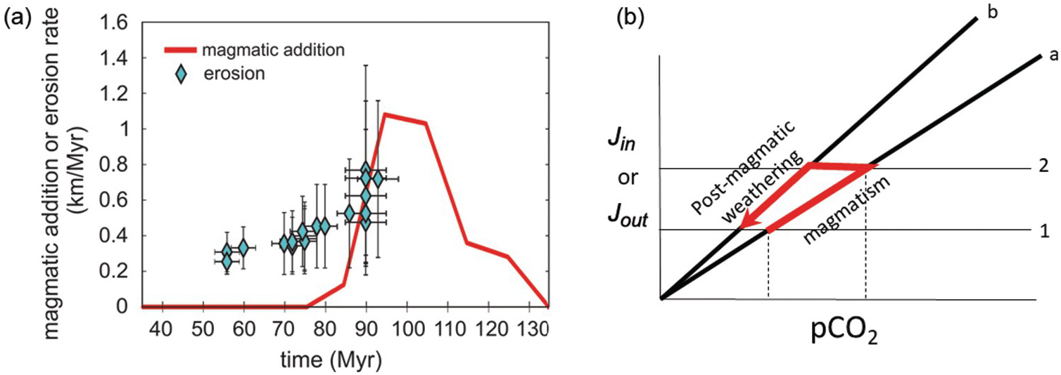
Ice sheets may also influence the long-term climate. Growth of ice sheets increases albedo, which cools the climate and encourages additional ice sheet growth. Could ice sheet expansion have further facilitated Cenozoic cooling by enhancing the silicate weathering associated with glacial erosion? This is a tantalizing thought as the Antarctic ice sheet is situated on the ancient Archean basement, raising the question of whether the onset of Antarctic glaciation at ~35 Ma may have played a role in the rise of seawater Sr isotopes at about the same time. On the other hand, glacial weathering might even result in the net production of CO2 through the oxidation of sulfides, which in turn drives carbonate dissolution; because the resulting acidity is driven by sulfide oxidation rather than carbonation itself, this results in a net release of CO2, counteracting the effects of glacial weathering and the ice–albedo positive feedback.Reference Tranter158, Reference Torres, Moosdorf, Hartmann, Adkins and West159
11.6.4 Climatic Excursions and Runaways
11.6.4.1 Hothouses
The Mesozoic–early Cenozoic greenhouse was punctuated by short-lived hothouse excursions, including the three oceanic anoxia events in the Cretaceous (OAE-1, -2, and -3) and the late PETM and surrounding hothouse excursions (“hyperthermals”).Reference Zachos, Pagani, Sloan, Thomas and Billups36, Reference Jenkyns, Forster, Schouten and Sinninghe Damste141, Reference Jenkyns160, Reference Slotnick161 Many of these excursions have in common an increase in temperature and pCO2, but different triggers. The PETM is characterized by a negative C isotope excursion, leading to suggestion that methane hydrates in the marine system were destabilized and released into the atmosphere.Reference Dickens, O’Neil, Rea and Owen35 Other mechanisms, such as destabilization of peat, opening of the North Atlantic Ocean, and even cometary impact,Reference Cramer and Kent162–Reference Storey, Duncan and Swisher164 have also been suggested for the PETM. Emplacement of the Caribbean flood basalt is thought to have driven Cretaceous OAE-2 at the Cenomanian–Turonian boundary,Reference Selby, Mutterlose and Condon165, Reference Leckie, Bralower and Cashman166 with volcanic release of CO2 leading to global warming, which in turn decreased the solubility of O2 in the ocean and setting conditions to be favorable for organic C preservation.Reference Leckie, Bralower and Cashman166
Hothouse excursions clearly have different triggers, but occur only during long-lived greenhouse baselines, not during icehouse baselines. Greenhouse baselines may be close to the threshold for hothouse excursions, such that any number of stochastic events could trigger an excursion if the system is close to threshold. The fact that hothouses return rapidly to baseline is further evidence that short-lived episodic events are responsible for triggering hothouses. Flood basalts, methane hydrate destabilization, and cometary impacts, among others, are all singular events that cannot sustain a long-term transition to a new steady state (unless the system is characterized by multiple steady states). These hothouse excursions all return to baseline because of the buffering effects of the silicate weathering feedback.
In some cases, excursions run away to a fundamentally different state. Unlike Earth, Venus is in a permanent hothouse. In part, this is due to continuous accumulation of CO2 or other greenhouse gases from the Venusian interior, enhanced by the fact that Venus has not had an efficient mechanism (e.g. weathering) for geologically sequestering C. The Venusian crust appears to be continually resurfaced, so the lack of weathering is not due to lack of a continuous supply of fresh material. Rather, surface conditions are so hot that water remains as a vapor, preventing the precipitation of liquid water to serve as a medium to dissolve rocks.Reference Ingersoll34 An explanation for Venus’s perpetual hothouse is that Venus crossed a threshold of atmospheric CO2, which resulted in enough warming to vaporize significant amounts of water. Water itself is an effective greenhouse gas, which further warms the atmosphere, in turn evaporating more water, until the system runs away to a new hothouse steady state. The greenhouse effect of water vapor on Earth is limited by the fact that water condenses and rains out, preventing runaway. Venus may have been more prone to cross this threshold because it lies closer to the sun.
11.6.4.2 Snowballs
During the Neoproterozoic and the early Paleoproterozoic, our planet appears to have almost completely frozen over (“Snowball”) based on the presence of low-latitude glacial sediments. In the Neoproterozoic, there were two or three Snowballs, which may have lasted 10–50 My.Reference Hoffman and Schrag7, Reference Hoffman, Kaufman, Halverson and Schrag8 During Neoproterozoic Snowball times, most of the continents were situated near the equator, which would have resulted in a strong ice–albedo feedback once ice sheets began to grow on these equatorial continents, ultimately leading to runaway glaciation.
It is generally agreed that the long-term baseline pCO2 during the Neoproterozoic was low, but why this was the case is debated. One hypothesis is that continents were preferentially at low latitudes and would thus have been characterized by higher silicate weathering kinetics. A recent variant of this hypothesis invokes emplacement of the Franklin large igneous province, which increased global weatherability due to the increased surface area of easily weathered basalt.Reference Cox167 Other hypotheses argue that continents were in a dispersed state during Neoproterozoic times, resulting in increased continental margins, which in turn accelerated biological productivity and enhanced the efficiency of C sequestration through organic C burial.Reference Hoffman and Schrag7, Reference Hoffman, Kaufman, Halverson and Schrag8 Highly positive seawater C isotopes predating the onset of the Snowball intervals are consistent with an unusually high fraction of organic C burial before each Snowball. Others have suggested that there was a paucity of continental arcs during the Neoproterozic, resulting in a decrease in global magmatic outputs.Reference McKenzie, Hughes, Gill and Myrow87, Reference McKenzie88, Reference Cao, Lee and Lackey145 Importantly, none of these scenarios is unique to the Neoproterozoic, which suggests that without the unique backdrop of low-latitude continents and low magmatic outputs, the conditions needed to cross the threshold would not otherwise have been met.
11.7 Summary and Further Research Directions
This chapter discussed the C cycling and long-term climate from a whole-Earth systems perspective. A conceptual framework for modeling C cycling between each reservoir was presented, along with a summary of the inventories of C in Earth’s major reservoirs and the fluxes of C between them. Long-term climate (>1 My) is controlled by the amount of C in the exogenic system (atmosphere, ocean, and biosphere), which itself is controlled by exchange between the endogenic (crust and mantle) and exogenic systems. Total exogenic C is controlled by outgassing from Earth’s interior via volcanism/metamorphism and sequestration of carbonate and organic C via silicate weathering and photosynthesis. The response time for silicate weathering is on the order of 100 ky, such that the amount of C in the exogenic system, and by implication climate, is at steady state on timescales longer than 1 My and endogenic inputs and exogenic outputs are balanced. Any long-term climate variability must reflect changing steady states, defined by temporal changes in the magnitude of volcanic and metamorphic inputs or in the efficiency (e.g. strength of weathering kinetics) of silicate weathering feedbacks, which draw down CO2 by precipitating carbonate. Silicate weathering serves as a negative feedback because CO2 drawdown increases with increasing pCO2 through a complex series of transfer functions, in which increasing pCO2 increases acidity and surface temperature, the latter of which increases precipitation and runoff, all of which enhance dissolution rates. Although tectonics and mantle dynamics drive endogenic outgassing, these endogenic processes can also enhance silicate weathering through tectonically driven erosion.
Long-term greenhouse intervals are likely driven by enhanced MOR spreading or the length of continental rifts and carbonate-intersecting continental arcs. Long-term icehouses have been widely thought to be driven by enhanced global weathering kinetics through an increase in orogenic activity, but decreased endogenic outgassing may be more important. Magmatic orogens may drive greenhouse intervals, but after magmatism ends, erosion and weathering of remnant topography increases global weathering kinetics, causing colder climates to immediately follow. The continental crust and CLM represent large repositories of C in the form of sediments, metamorphic C in the crust, and metasomatized domains in the lithospheric mantle. This continental C can be periodically tapped during rifting and continental arc magmatism, leading to greenhouse states. Below, we list several questions to guide future research.
What controls baseline C in the exogenic system and hence climate? Specifically, what is more effective in changing baseline C: changes in source or in the efficiency of the sink?Reference Godderis and Francois168 What are the relative roles of MORs, plumes, continental arcs, continental rifts, and orogens in controlling C inputs? How do global weathering kinetics change with time or with changes in the nature of Earth’s surface? What is the functional form of the silicate weathering feedback? Are orogens net regional sources or sinks of C?
How has the lithospheric (crust + lithospheric mantle) reservoir of C changed through time? The answer to this question is key to quantifying how mantle degassing and metamorphic fluxes change with time. Progress may come from characterizing average amounts of carbonate and graphite in igneous and metamorphic basement rocks (see Ref. Reference White, Schulz, Lowenstern, Vivit and Bullen169). It will also be important to build a more quantitative budget of carbonate- and organic C-bearing sediments on the continents (see Ref. Reference Husson and Peters170).
How has the spatial and temporal distribution of C deposition changed through time? Specifically, how has C deposition been partitioned between the shallow and deep sea through time? Also of interest is whether organic C and carbonate remain coupled during sedimentary deposition; if not, the bulk redox state of total C will vary regionally, with implications for the redox state of subducted materials.
How did early Earth volatile cycles operate? During much of Earth’s history, atmospheric oxygen levels were low. Questions thus arise as to whether CO2 or some other carbon species, such as methane, was the dominant greenhouse gas during those times. Were Archean atmospheric CO2 contents much higher than today, as seems to be required by a lower solar luminosity (a faint young sun)?Reference Sagan and Mullen1 If other greenhouse gases were more important in the Archean, how would weathering feedbacks have behaved?
How have changes in the nature of the C cycle influenced the cycling of other elements on Earth? The dominant form of di-oxygen (O2) production on Earth is through photosynthetic reduction of CO2 to organic C. The evolution of atmospheric O2 is thus controlled by the C cycle. Oxygen availability in turn influences the geochemical behaviors of redox-sensitive elements, such as S, N, and metals, as well as elements like P that complex with or absorb onto metals of a certain oxidation state.
We conclude our review with the caveat that what we have discussed here is strongly biased by our experiences on Earth. Nevertheless, the concepts presented here should be transportable to understanding element cycles and climates on other planets in our solar system or beyond.
Acknowledgments
This work was supported by the US NSF Frontiers of Earth Systems Dynamics grant (OCE-1338842) and a NASA grant 80NSSC18K0828. We thank the organizers Craig Manning and Isabelle Daniel of the 2018 Deep Carbon Science Gordon Research Conference in Rhode Island for providing inspiration. We also thank L. Carter, D. Catling, M. Edmonds, J. Eguchi, D. Grewal, M. Kastner, A. Lenardic, T. Lyons, D. Müller, T. Plank, K. Siebach, J. Tucker, A. J. West, and L. Yeung for various insights. We thank Jeremy Caves for his insightful review.


 Open access