


Impact Statement
Electro-osmosis appears ubiquitously in nanofluidic devices where an external voltage is applied. We show that a widely employed approximate expression used to estimate electro-osmosis from selectivity and ion current violates fluid-dynamics scaling arguments. Nevertheless, for very narrow biological pores often used in nanopore sensing devices, it still captures the order of magnitude of electro-osmotic flow (EOF), making it a useful tool for preliminary nanofluidic device design. We also show, through atomistic simulations, specific cases where selectivity does not correlate with EOF. Currently, it is relatively easy to alter the nanopore surface charge, allowing biotechnological labs to produce a wide variety of surface charge patterns. Hence, we expect that our findings on the assessment of the validity of approximate estimation of EOF will contribute to developing a more fluid-dynamically consistent methodology for nanopore engineering.
1. Introduction
Membranes are widely employed in several industrial processes due to their selective permeability and their ability to separate substances at the molecular level. They are used in desalination (Amy et al. Reference Amy, Ghaffour, Li, Francis, Linares, Missimer and Lattemann2017) and in ion separation (Jian et al. Reference Jian, Qiu, Xia, Lu, Chen, Gu, Liu, Hu, Qu, Wang and Zhang2020). Additionally, membranes present opportunities for energy production via salinity gradient power generation, also sometimes indicated as blue energy, where the free energy difference between freshwater and seawater is converted in electric energy (Baldelli et al. Reference Baldelli, Di Muccio, Viola, Giacomello, Cecconi, Balme and Chinappi2024; Wang et al. Reference Wang, Wang and Elimelech2022). Another application of nanoporous membranes is nanopore sensing. In the most common set-up, the membrane separates two reservoirs containing an electrolyte solution where the molecules to be detected are placed. A single nanopore connects the two reservoirs and the molecule is recognized by the alteration of the electric conductance due to its interaction with the nanopore (Chinappi & Cecconi Reference Chinappi and Cecconi2018; Varongchayakul et al. Reference Varongchayakul, Song, Meller and Grinstaff2018).
A common feature of the transport phenomena through nanoporous membranes is the complex coupling between mass, species and charge transport (Marbach & Bocquet Reference Marbach and Bocquet2019). Depending on the application, the two reservoirs that are separated by the membrane may have a different electric potential (as in nanopore sensing), different ion concentrations (as in salinity gradient energy harvesting) or different pressure. The surface of the nanopore is usually charged, an occurrence that typically favours the passage of ions bearing charges that are opposite to the surface (counterions), and hindering ions carrying a charge of the same sign of the nanopore surface (coions). This means that, for instance, a fluid flow induced by a pressure difference will drag a different number of coions and counterions resulting in an electric current, while imposing a difference in ion concentration may result in an electric current due to the preferential passage of counterions. For a discussion of the various electrohydrodynamic couplings between pressure, voltage and concentration difference load, we refer the reader to the review by Marbach & Bocquet (Reference Marbach and Bocquet2019).
In this work, we focus on a specific electrohydrodynamic coupling: the EOF. Electro-osmotic flow is the net transport of an electrolyte solution induced by an applied voltage (Bruus Reference Bruus2008; Gubbiotti et al. Reference Gubbiotti, Baldelli, Di Muccio, Malgaretti, Marbach and Chinappi2022). Electro-osmosis is often used to actuate fluids in microfluidic and nanofluidic devices (Haywood et al. Reference Haywood, Saha-Shah, Baker and Jacobson2015; Wu et al. Reference Wu, Ramiah Rajasekaran and Martin2016) and it affects the ionic conduction of nanopores (Balme et al. Reference Balme, Picaud, Manghi, Palmeri, Bechelany, Cabello-Aguilar, Abou-Chaaya, Miele, Balanzat and Janot2015; Yusko et al. Reference Yusko, An and Mayer2009). Recently, EOF emerged as a promising approach in nanopore sensing applications to control the transport of molecules from the bulk of the reservoir to the nanopore sensor (Asandei et al. Reference Asandei, Schiopu, Chinappi, Seo, Park and Luchian2016; Bhamidimarri et al. Reference Bhamidimarri, Prajapati, van den Berg, Winterhalter and Kleinekathöfer2016; Boukhet et al. Reference Boukhet, Piguet, Ouldali, Pastoriza-Gallego, Pelta and Oukhaled2016; Chinappi et al. Reference Chinappi, Yamaji, Kawano and Cecconi2020; Huang et al. Reference Huang, Willems, Soskine, Wloka and Maglia2017; Niu et al. Reference Niu, Li, Ying and Long2022; Saharia et al. Reference Saharia, Bandara, Karawdeniya, Hammond, Alexandrakis and Kim2021; Wen et al. Reference Wen, Bertosin, Shi, Dekker and Schmid2022) and to control molecule translocation through the nanopore (Ermann et al. Reference Ermann, Hanikel, Wang, Chen, Weckman and Keyser2018; Hsu & Daiguji Reference Hsu and Daiguji2016; Sauciuc et al. Reference Sauciuc, Morozzo della Rocca, Tadema, Chinappi and Maglia2023; Yu et al. Reference Yu, Kang, Li, Mehrafrooz, Makhamreh, Fallahi and Wanunu2023).
Here, we focus on EOF due to a time-independent external voltage and we restrict our analysis to single nanopores or membranes made by a regular array of nanopores. In this framework, the simplest (but not the only) route to get EOF is the presence of a fixed surface charge at the nanopore wall. Indeed, nanopore surface charge affects the concentration of the dissolved ion species, inducing local charge accumulation even in a fluid which is globally neutral. For instance, a negative surface charge will attract positive ions (that, in this case, are the counterions) and repel negative ions (coions), see figure 1(a). When a voltage is applied between the two reservoirs, an external electric field funnels into the pore. This electric field exerts a net force on the charged portions of fluid that, in turn, set the fluid in motion. Although continuum electrohydrodynamics is not valid in narrow nanopores, some concepts are instrumental to understand the basic principles of EOF. In this respect, a relevant quantity is the Debye length $\lambda _D$
(figure 1
a), which gives an indication of the thickness of the layer close to the charged walls where the accumulation of counterions and the depletion of coions takes places. For diluted solutions,
$\lambda _D$
(figure 1
a), which gives an indication of the thickness of the layer close to the charged walls where the accumulation of counterions and the depletion of coions takes places. For diluted solutions,
 \begin{equation} \lambda _D = \sqrt { \frac {\varepsilon _0 \varepsilon _r k_BT}{e^2\sum \limits _\alpha c_\alpha Z_\alpha ^2} } \; , \end{equation}
where $T$
is temperature,
$T$
is temperature, $k_B$
the Boltzmann constant,
$k_B$
the Boltzmann constant, $\varepsilon _0$
vacuum permittivity,
$\varepsilon _0$
vacuum permittivity, $\varepsilon _r$
relative permittivity,
$\varepsilon _r$
relative permittivity, $e$
the elementary charge and
$e$
the elementary charge and $c_\alpha$
and
$c_\alpha$
and $Z_\alpha$
are, respectively, the number concentration and valency of the ionic species
$Z_\alpha$
are, respectively, the number concentration and valency of the ionic species $\alpha$
in solution, e.g.
$\alpha$
in solution, e.g. $z_{\alpha } = +1$
for
$z_{\alpha } = +1$
for $K^+$
and
$K^+$
and $z_{\alpha } = -1$
for
$z_{\alpha } = -1$
for $Cl^-$
. For a derivation of (1) we refer the reader to standard microfluidics textbooks such as, for instance, Bruus (Reference Bruus2008).
$Cl^-$
. For a derivation of (1) we refer the reader to standard microfluidics textbooks such as, for instance, Bruus (Reference Bruus2008).
In typical nanopore applications, with KCl water solutions at $300$
K,
$300$
K, $\lambda _D$
ranges from
$\lambda _D$
ranges from $\,0.3\,\mathrm{nm}$
for
$\,0.3\,\mathrm{nm}$
for $1\,\textrm{M}$
KCl to
$1\,\textrm{M}$
KCl to $10\,\mathrm{nm}$
for
$10\,\mathrm{nm}$
for $1\,\textrm{mM}$
KCl. It is worth noting that, even if
$1\,\textrm{mM}$
KCl. It is worth noting that, even if $\lambda _D$
is usually in the nanometric (or subnanometric) range, for nanopore membranes it may be comparable with the pore diameter, in particular for the biological pores used in nanopore sensing (Boukhet et al. Reference Boukhet, Piguet, Ouldali, Pastoriza-Gallego, Pelta and Oukhaled2016; Bétermier et al. Reference Bétermier, Cressiot, Di Muccio, Jarroux, Bacri, Morozzo Della Rocca and Tarascon2020; Manrao et al. Reference Manrao, Derrington, Laszlo, Langford, Hopper, Gillgren, Pavlenok, Niederweis and Gundlach2012; Mayer et al. Reference Mayer, Cao and Dal Peraro2022; Straathof et al. Reference Straathof, Di Muccio, Yelleswarapu, Alzate Banguero, Wloka, van der Heide, Chinappi and Maglia2023).
$\lambda _D$
is usually in the nanometric (or subnanometric) range, for nanopore membranes it may be comparable with the pore diameter, in particular for the biological pores used in nanopore sensing (Boukhet et al. Reference Boukhet, Piguet, Ouldali, Pastoriza-Gallego, Pelta and Oukhaled2016; Bétermier et al. Reference Bétermier, Cressiot, Di Muccio, Jarroux, Bacri, Morozzo Della Rocca and Tarascon2020; Manrao et al. Reference Manrao, Derrington, Laszlo, Langford, Hopper, Gillgren, Pavlenok, Niederweis and Gundlach2012; Mayer et al. Reference Mayer, Cao and Dal Peraro2022; Straathof et al. Reference Straathof, Di Muccio, Yelleswarapu, Alzate Banguero, Wloka, van der Heide, Chinappi and Maglia2023).
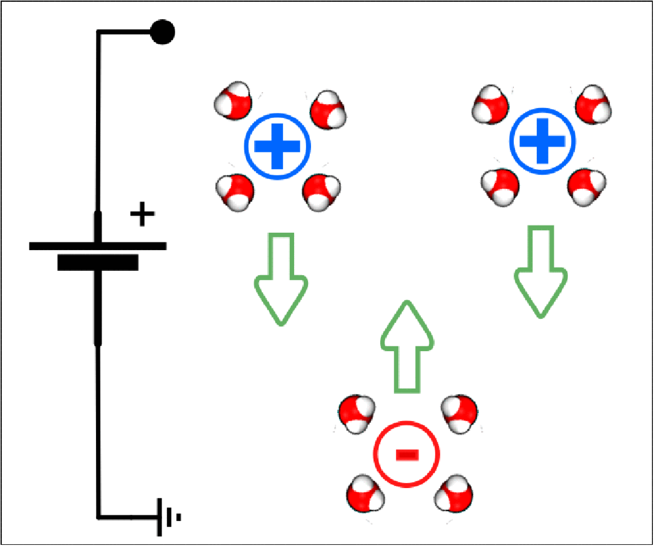
Electro-osmotic flow in nanopores and its connection with selectivity. (a) Sketch of the continuum electrohydrodynamic model for EOF in cylindrical nanopores. A typical nanopore sensing device is constituted by a single nanopore embedded in a membrane. The nanopore connects two reservoirs that, as usual in the electrophysiology and nanopore sensing field, are here indicated as cis and trans. One of the two reservoirs is grounded (in our case, cis) and a voltage $\Delta V$
is applied at the trans side. Moreover, different ion concentrations can be present in the two reservoirs resulting in a concentration difference
$\Delta V$
is applied at the trans side. Moreover, different ion concentrations can be present in the two reservoirs resulting in a concentration difference $\Delta C_i$
, with i the ion species. Here, we consider only the case when the electrolyte is of the same kind at the cis and trans sides and it is obtained dissolving a salt; consequently, the salt concentration difference
$\Delta C_i$
, with i the ion species. Here, we consider only the case when the electrolyte is of the same kind at the cis and trans sides and it is obtained dissolving a salt; consequently, the salt concentration difference $\Delta C$
is the only relevant parameter to define the concentration differences of all the ions. Fixed charges are present at the nanopore surface, resulting in an equilibrium (
$\Delta C$
is the only relevant parameter to define the concentration differences of all the ions. Fixed charges are present at the nanopore surface, resulting in an equilibrium ( $\Delta V = 0$
,
$\Delta V = 0$
, $\Delta C = 0$
) distribution of ion charge in the pore. Under a voltage load
$\Delta C = 0$
) distribution of ion charge in the pore. Under a voltage load $\Delta V$
, this charge accumulation typically results in two effects: (i) the pore is selective for positive (cation) or negative (anion) species and (ii) an EOF sets in. The EOF is due to the net force that the ions transfer to the fluid under an external
$\Delta V$
, this charge accumulation typically results in two effects: (i) the pore is selective for positive (cation) or negative (anion) species and (ii) an EOF sets in. The EOF is due to the net force that the ions transfer to the fluid under an external $\Delta V$
. If the pore is negatively charged (as in the figure), positive ions accumulate in the pore, and the axial component of electric field acts on the positive ions that, in turn, transfers momentum to the fluid putting it in motion. Panel (a) refers to a condition where
$\Delta V$
. If the pore is negatively charged (as in the figure), positive ions accumulate in the pore, and the axial component of electric field acts on the positive ions that, in turn, transfers momentum to the fluid putting it in motion. Panel (a) refers to a condition where $\Delta C = 0$
so that the Debye length
$\Delta C = 0$
so that the Debye length $\lambda _D$
is the same in any region of the system. (b) Pictorial view of the Gu et al. (Reference Gu, Cheley and Bayley2003) model, showing the EOF originated from the transport of the water molecules around each ion. The main limitation of the model is that it does not account for the viscous drag that will put in motion the fluid also in the uncharged portion of the pore lumen. (c) The GHK model: selectivity measurement from reversal potential. The EOF in single nanopores cannot be directly measured. Moreover, also cation and anion contributions to the total current
$\lambda _D$
is the same in any region of the system. (b) Pictorial view of the Gu et al. (Reference Gu, Cheley and Bayley2003) model, showing the EOF originated from the transport of the water molecules around each ion. The main limitation of the model is that it does not account for the viscous drag that will put in motion the fluid also in the uncharged portion of the pore lumen. (c) The GHK model: selectivity measurement from reversal potential. The EOF in single nanopores cannot be directly measured. Moreover, also cation and anion contributions to the total current $I$
are not directly accessible. An accessible quantity is, instead, the reversal potential
$I$
are not directly accessible. An accessible quantity is, instead, the reversal potential $V_r$
that is the applied voltage at which, in presence of a
$V_r$
that is the applied voltage at which, in presence of a $\Delta C$
, the electric current is zero. (d) Sketches of the directions of the ionic flows in the case of a
$\Delta C$
, the electric current is zero. (d) Sketches of the directions of the ionic flows in the case of a $1:1$
electrolyte for (i)
$1:1$
electrolyte for (i) $\Delta V = 0$
and (ii)
$\Delta V = 0$
and (ii) $\Delta V = V_r$
.
$\Delta V = V_r$
.

2. Experimental measurements of EOF in nanopores: why direct methods are challenging
Measuring flow rates at the microscale and nanoscale is extremely challenging. For large membranes containing millions of nanopores, the flow rate can be so high that it can be directly measured, see, for instance, the microlitre per minute rates observed in Whitby et al. (Reference Whitby, Cagnon, Thanou and Quirke2008) and Wu et al. (Reference Wu, Ramiah Rajasekaran and Martin2016). However, for single nanopores, dedicated approaches need to be developed as it is not possible to directly measure the flow rate. Moreover, extrapolations of the single-pore flow rate from experiments with multipore membranes are not straightforward since the interaction among neighbouring pores results in a nonlinear scaling of the flow rate with the number of nanopores (Baldelli et al. Reference Baldelli, Di Muccio, Viola, Giacomello, Cecconi, Balme and Chinappi2024; Gadaleta et al. Reference Gadaleta, Sempere, Gravelle, Siria, Fulcrand, Ybert and Bocquet2014). An interesting approach for single nanopore flow measurements was reported in Secchi et al. (Reference Secchi, Marbach, Niguès, Stein, Siria and Bocquet2016), where the flow rate through carbon and boron nitride nanotubes of radius $\gt 10$
nm was measured by tracking particles outside the nanopore and comparing their trajectories with numerical solution of the Landau–Squire nanojet, see also Secchi et al. (Reference Secchi, Marbach, Niguès, Siria and Bocquet2017). However, this approach cannot be easily extended to smaller pores and, in particular, to pores embedded in a membrane. Indeed, differently from the Landau–Squire plume, the velocity of the funnel-like flow field far from a nanopore embedded in a membrane scales as
$\gt 10$
nm was measured by tracking particles outside the nanopore and comparing their trajectories with numerical solution of the Landau–Squire nanojet, see also Secchi et al. (Reference Secchi, Marbach, Niguès, Siria and Bocquet2017). However, this approach cannot be easily extended to smaller pores and, in particular, to pores embedded in a membrane. Indeed, differently from the Landau–Squire plume, the velocity of the funnel-like flow field far from a nanopore embedded in a membrane scales as $(d/r)^2$
, where
$(d/r)^2$
, where $d$
is the pore diameter. Consequently, after a few
$d$
is the pore diameter. Consequently, after a few $\unicode{x03BC}\mathrm{m}$
s from the nanopore exit, the velocity would be so low that particle tracking cannot be used to reliably estimate the velocity field. As an example, for a nanopore diameter of 2 nm (as several biological pores), even assuming a speed
$\unicode{x03BC}\mathrm{m}$
s from the nanopore exit, the velocity would be so low that particle tracking cannot be used to reliably estimate the velocity field. As an example, for a nanopore diameter of 2 nm (as several biological pores), even assuming a speed $v_0 = 1$
ms at the nanopore exit, at a distance of
$v_0 = 1$
ms at the nanopore exit, at a distance of $2\,\unicode{x03BC}\mathrm{m}$
from the nanopore the velocity would be
$2\,\unicode{x03BC}\mathrm{m}$
from the nanopore the velocity would be $\simeq 1\,\unicode{x03BC}\mathrm{m\,s}^{-1}$
while at
$\simeq 1\,\unicode{x03BC}\mathrm{m\,s}^{-1}$
while at $10\,\unicode{x03BC}\mathrm{m}$
from the pore it would be reduced to
$10\,\unicode{x03BC}\mathrm{m}$
from the pore it would be reduced to $\simeq 10^{-2}\,\unicode{x03BC}\mathrm{m\,s}^{-1}$
. Other interesting anemometry techniques were reported by Laohakunakorn et al. (Reference Laohakunakorn, Gollnick, Moreno-Herrero, Aarts, Dullens, Ghosal and Keyser2013), where the flow rate of a Landau–Squire nanojet for a glass nanopipette of radius
$\simeq 10^{-2}\,\unicode{x03BC}\mathrm{m\,s}^{-1}$
. Other interesting anemometry techniques were reported by Laohakunakorn et al. (Reference Laohakunakorn, Gollnick, Moreno-Herrero, Aarts, Dullens, Ghosal and Keyser2013), where the flow rate of a Landau–Squire nanojet for a glass nanopipette of radius $75$
nm was measured and by Mc Hugh et al. (Reference Mc Hugh, Andresen and Keyser2019); however, also in these cases, the extension of these approaches to smaller pores appear extremely challenging.
$75$
nm was measured and by Mc Hugh et al. (Reference Mc Hugh, Andresen and Keyser2019); however, also in these cases, the extension of these approaches to smaller pores appear extremely challenging.
Since measuring flow rates is challenging at the nanoscale, while measuring electric current is more feasible (standard patch clamp instruments typically used in nanopore sensing are able to reach a picoamp resolution), one may be tempted to use Onsager-like relations, at least in the linear regime, to estimate EOF from the measurement of the streaming current. More specifically, the following relation holds (Mazur & Overbeek Reference Mazur and Overbeek1951):
 \begin{equation} \left ( \frac {I}{\Delta P} \right )_{\Delta V = 0} = \left ( \frac {Q_{eo}}{\Delta V} \right )_{\Delta P = 0}, \end{equation}
where $I$
is the electric current flowing through the system under the action of an applied pressure difference
$I$
is the electric current flowing through the system under the action of an applied pressure difference $\Delta P$
(at
$\Delta P$
(at $\Delta V = 0$
), while
$\Delta V = 0$
), while $Q_{eo}$
is the volumetric EOF rate under an applied voltage
$Q_{eo}$
is the volumetric EOF rate under an applied voltage $\Delta V$
(at
$\Delta V$
(at $\Delta P = 0$
). For the derivation of (2), we refer readers to the original article by Mazur & Overbeek (Reference Mazur and Overbeek1951) while an explicit calculation of the transport coefficients is possible for some specific cases, such as smoothly corrugated channels, see Malgaretti et al. (Reference Malgaretti, Janssen, Pagonabarraga and Rubi2019). Despite (2) being promising, as it allows estimating the flow rate from an electric current measurement, it cannot be applied to a wide class of nanopores. For instance, for biological nanopores atomistic simulations indicate that
$\Delta P = 0$
). For the derivation of (2), we refer readers to the original article by Mazur & Overbeek (Reference Mazur and Overbeek1951) while an explicit calculation of the transport coefficients is possible for some specific cases, such as smoothly corrugated channels, see Malgaretti et al. (Reference Malgaretti, Janssen, Pagonabarraga and Rubi2019). Despite (2) being promising, as it allows estimating the flow rate from an electric current measurement, it cannot be applied to a wide class of nanopores. For instance, for biological nanopores atomistic simulations indicate that $Q_{eo}$
may reach the order of tens of water molecules per ns under a voltage of
$Q_{eo}$
may reach the order of tens of water molecules per ns under a voltage of $100$
mV, resulting in
$100$
mV, resulting in
 \begin{equation} \left ( \frac {I}{\Delta P} \right )_{\Delta V = 0} = \left ( \frac {Q_{eo}}{\Delta V} \right )_{\Delta P = 0} \sim 10^{-19} \, {\rm \frac {m^3}{s V}} \, , \end{equation}
which implies that a pressure difference $\Delta P \sim 10^7$
Pa is needed for a current of just 1 pA. Lipidic or polymeric membranes normally used in biological nanopore experiments cannot sustain such a high pressure making, de facto, this Onsager-like approach unfeasible to estimate EOF. Solid-state membranes can sustain larger pressures with respect to lipid membranes and studies where a
$\Delta P \sim 10^7$
Pa is needed for a current of just 1 pA. Lipidic or polymeric membranes normally used in biological nanopore experiments cannot sustain such a high pressure making, de facto, this Onsager-like approach unfeasible to estimate EOF. Solid-state membranes can sustain larger pressures with respect to lipid membranes and studies where a $\Delta P \simeq 1$
atm is applied between the two reservoirs can be found in the literature, see, e.g. Hoogerheide et al. (Reference Hoogerheide, Lu and Golovchenko2014), J. Li et al. (Reference Li, Hu, Li, Tong, Yu and Zhao2017) and Lu et al. (Reference Lu, Hoogerheide, Zhao, Zhang, Tang, Yu and Golovchenko2013). Moreover, nanopores in solid-state membranes can be much larger than biological nanopores. For instance, in the above-mentioned studies, the pore diameter is
$\Delta P \simeq 1$
atm is applied between the two reservoirs can be found in the literature, see, e.g. Hoogerheide et al. (Reference Hoogerheide, Lu and Golovchenko2014), J. Li et al. (Reference Li, Hu, Li, Tong, Yu and Zhao2017) and Lu et al. (Reference Lu, Hoogerheide, Zhao, Zhang, Tang, Yu and Golovchenko2013). Moreover, nanopores in solid-state membranes can be much larger than biological nanopores. For instance, in the above-mentioned studies, the pore diameter is $\simeq 10$
nm. This larger size, for highly charged pores, may result in a relatively large streaming current (and EOF) that, in principle, may allow the direct application of (3) for the estimation of EOF although, to the best of our knowledge, this approach has not been used for single nanopores.
$\simeq 10$
nm. This larger size, for highly charged pores, may result in a relatively large streaming current (and EOF) that, in principle, may allow the direct application of (3) for the estimation of EOF although, to the best of our knowledge, this approach has not been used for single nanopores.
2.1 Measurement of selectivity: the reversal potential
The difficulties in measuring EOF in experiments brought several authors to find alternative ways to get indications of the possible presence and direction of EOF. A quite popular reasoning to connect cation/anion selectivity with EOF appeared in the literature (Gu et al. Reference Gu, Cheley and Bayley2003). The argument is as follows: if a pore is selective for anions, under a $\Delta V$
, the anion current
$\Delta V$
, the anion current $I^-$
will be larger than the cationic one
$I^-$
will be larger than the cationic one $I^+$
. Since each ion drags a coordination shell of water molecules, the imbalance in anion/cation flow will result in a EOF. We will discuss in detail the problems of this approach in the next sections. For now, we want to stress which are the main merits of this argument and its consequence in the literature. Selectivity can be estimated by relatively simple experiments. Indeed, if the two reservoirs are at a different salt concentrations and the membrane is selective for anions (or cations), the diffusive fluxes of anions and cations will be different resulting in an electric current even at
$I^+$
. Since each ion drags a coordination shell of water molecules, the imbalance in anion/cation flow will result in a EOF. We will discuss in detail the problems of this approach in the next sections. For now, we want to stress which are the main merits of this argument and its consequence in the literature. Selectivity can be estimated by relatively simple experiments. Indeed, if the two reservoirs are at a different salt concentrations and the membrane is selective for anions (or cations), the diffusive fluxes of anions and cations will be different resulting in an electric current even at $\Delta V = 0$
. This current is often indicated as the osmotic current in the literature on salinity gradient power generation (Laucirica et al. Reference Laucirica, Toimil-Molares, Trautmann, Marmisollé and Azzaroni2021). If a voltage
$\Delta V = 0$
. This current is often indicated as the osmotic current in the literature on salinity gradient power generation (Laucirica et al. Reference Laucirica, Toimil-Molares, Trautmann, Marmisollé and Azzaroni2021). If a voltage $\Delta V$
is also applied, there will be a specific voltage
$\Delta V$
is also applied, there will be a specific voltage $V_r$
for which the current is zero. This voltage is commonly indicated as the reversal potential
$V_r$
for which the current is zero. This voltage is commonly indicated as the reversal potential $V_r$
. The sign of
$V_r$
. The sign of $V_r$
depends on the anion/cation selectivity of the pore, see figure 1(c). The measurement of the reversal potential is relatively simple and it is commonly used in nanopore manuscripts to characterize the selectivity. Once
$V_r$
depends on the anion/cation selectivity of the pore, see figure 1(c). The measurement of the reversal potential is relatively simple and it is commonly used in nanopore manuscripts to characterize the selectivity. Once $V_r$
is measured, standard simplified models allow us to extract the permeability ratio
$V_r$
is measured, standard simplified models allow us to extract the permeability ratio $P_+/P_-$
, that is the ratio between cation and anion flows under the action of a difference of electrochemical potential. A common approach to connect
$P_+/P_-$
, that is the ratio between cation and anion flows under the action of a difference of electrochemical potential. A common approach to connect $V_r$
to
$V_r$
to $P_+/P_-$
is by means of the Goldman–Hodgkin–Katz (GHK) model (Goldman Reference Goldman1943; Hodgkin & Katz Reference Hodgkin and Katz1949) that, for
$P_+/P_-$
is by means of the Goldman–Hodgkin–Katz (GHK) model (Goldman Reference Goldman1943; Hodgkin & Katz Reference Hodgkin and Katz1949) that, for $1:1$
electrolytes (such as KCl or NaCl), provides the expression
$1:1$
electrolytes (such as KCl or NaCl), provides the expression
 \begin{equation} \frac {P_+}{P_-} = \frac {C^t_- - C^c_- \exp {\left ( e \beta V_r \right ) } } {C^t_+ \exp {\left ( e \beta V_r \right ) - C^c_+ } } \; , \end{equation}
where $C^t$
and
$C^t$
and $C^c$
are the salt concentrations at the trans and cis reservoir, respectively. For completeness, we reported the derivation of GHK equation in Supplementary Note S1. The GHK model is a simplified theoretical model of the transport, and, as such, it is not the only possibility to link the permeability ratio to the reversal potential
$C^c$
are the salt concentrations at the trans and cis reservoir, respectively. For completeness, we reported the derivation of GHK equation in Supplementary Note S1. The GHK model is a simplified theoretical model of the transport, and, as such, it is not the only possibility to link the permeability ratio to the reversal potential $V_r$
. In membrane science, another approach to estimate the membrane potential is also used, in particular in manuscripts on blue-energy harvesting (Baldelli et al. Reference Baldelli, Di Muccio, Viola, Giacomello, Cecconi, Balme and Chinappi2024; Laucirica et al. Reference Laucirica, Toimil-Molares, Trautmann, Marmisollé and Azzaroni2021). The comparison between the two approaches is not within the aims of the present manuscript. We refer the reader to a recent work by Zhang et al. (Reference Zhang, Wang, Yaroshchuk, Du, Xin, Bruening and Xia2024) for an interesting discussion.
$V_r$
. In membrane science, another approach to estimate the membrane potential is also used, in particular in manuscripts on blue-energy harvesting (Baldelli et al. Reference Baldelli, Di Muccio, Viola, Giacomello, Cecconi, Balme and Chinappi2024; Laucirica et al. Reference Laucirica, Toimil-Molares, Trautmann, Marmisollé and Azzaroni2021). The comparison between the two approaches is not within the aims of the present manuscript. We refer the reader to a recent work by Zhang et al. (Reference Zhang, Wang, Yaroshchuk, Du, Xin, Bruening and Xia2024) for an interesting discussion.
2.2. Connection between selectivity and EOF
There is no general way to obtain EOF from reversal potential experiments. Indeed, even in a linear response approximation, the EOF is related to the streaming current (i.e. the electric current under the action of an applied pressure) and not to the reversal potential (that is measured when different concentrations are applied at the two sides of the membrane), as we noted in §2. However, as anticipated, a quite popular expression is often used in the literature to estimate the EOF from the permeability ratio. The expression, which, to the best of our knowledge, was introduced by Gu et al. (Reference Gu, Cheley and Bayley2003) and derived in the following.
The basic assumption in Gu et al. (Reference Gu, Cheley and Bayley2003) is that every ion carries a shell of $N_{w,i}$
water molecules, where the subscript
$N_{w,i}$
water molecules, where the subscript $i$
indicates the ionic species. The number of ions of the ith species flowing through the pore per unit of time is indicated as
$i$
indicates the ionic species. The number of ions of the ith species flowing through the pore per unit of time is indicated as $Q_i$
. Without loss of generality, we will consider
$Q_i$
. Without loss of generality, we will consider $Q_i$
positive if the flow is from the trans to the cis reservoir. The EOF, expressed in terms of number of water molecules flowing through the pore per unit of time, is hence given by
$Q_i$
positive if the flow is from the trans to the cis reservoir. The EOF, expressed in terms of number of water molecules flowing through the pore per unit of time, is hence given by
 \begin{equation} Q_{eof,n} = \sum _i^{N_s} N_{w,i} \, Q_i , \end{equation}
where $N_s$
is the number of ionic species. Here
$N_s$
is the number of ionic species. Here $Q_i$
is not an experimentally accessible quantity, so, (5) needs to be rearranged.
$Q_i$
is not an experimentally accessible quantity, so, (5) needs to be rearranged.
It is worth noting that the above-mentioned mechanism differs from the established mechanism for EOF in pores, where, briefly, the accumulation of motile ions in the pore region is affected by the component of the electric field parallel to the pore axis, resulting in an electrohydrodynamic force that drives fluid motion via viscous forces, also where the net charge is zero (Bruus Reference Bruus2008; Gubbiotti et al. Reference Gubbiotti, Baldelli, Di Muccio, Malgaretti, Marbach and Chinappi2022). Instead, (5) describes just a sort of kinematic mechanism where the ions drag their hydration layers, neglecting any water flow in the electroneutral part of the nanopore.
In the typical case in nanopore sensing experiments, where the electrolyte solution is mainly constituted by an anion and a cation species (e.g. KCl, NaCl), (5) becomes
 \begin{equation} Q_{eof,n} = N_{(w,+)} \, Q_+ + N_{(w,-)} \, Q_- \, . \end{equation}
The electric current $I$
can also be expressed in terms of
$I$
can also be expressed in terms of $Q_+$
and
$Q_+$
and $Q_-$
as
$Q_-$
as
 \begin{equation} I = e \left ( z_+ Q_{+} + z_- Q_- \right ) , \end{equation}
with $e$
the elementary charge and
$e$
the elementary charge and $z_i$
the valency, e.g.
$z_i$
the valency, e.g. $z_{Cl^-} = -1$
,
$z_{Cl^-} = -1$
, $z_{K^+} = 1$
. Combining (6) and (7), we get
$z_{K^+} = 1$
. Combining (6) and (7), we get
 \begin{equation} Q_{eof,n} = \frac {I}{e} \frac {N_{(w,+)} \, Q_{+} + N_{(w,-)} \, Q_-} {z_+ Q_{+} + z_- Q_-} \, . \end{equation}
Dividing by $Q_-$
and considering that
$Q_-$
and considering that $P_{+}/P_{-} = - Q_+/Q_-$
(the minus on the right-hand side stems from the fact that the permeabilities are defined as positive quantities, while the signs of the ion flow rates depend on the direction of the flow), (8) can be rewritten as
$P_{+}/P_{-} = - Q_+/Q_-$
(the minus on the right-hand side stems from the fact that the permeabilities are defined as positive quantities, while the signs of the ion flow rates depend on the direction of the flow), (8) can be rewritten as
 \begin{equation} Q_{eof,n} = \frac {I}{e} \frac { N_{(w,+)} \, \frac {P_{+}}{P_-} - N_{(w,-)}} {z_+ \frac {P_{+}}{P_-} - z_-} \, , \end{equation}
that, for a $1:1$
electrolyte (
$1:1$
electrolyte ( $z_+ = 1$
,
$z_+ = 1$
, $z_- = -1$
) and further assuming that
$z_- = -1$
) and further assuming that $N_w$
is the same for anions and cations (an occurrence somehow reasonable for KCl, since
$N_w$
is the same for anions and cations (an occurrence somehow reasonable for KCl, since $K^+$
and
$K^+$
and $Cl^+$
have the same mobility, but less justified for NaCl) reduces to
$Cl^+$
have the same mobility, but less justified for NaCl) reduces to
 \begin{equation} Q_{eof,n} = N_w \frac {I}{e} \frac { \frac {P_{+}}{P_-} - 1} { \frac {P_{+}}{P_-} + 1} \, , \end{equation}
that is the expression derived in Gu et al. (Reference Gu, Cheley and Bayley2003) and used in several papers, see, among others Asandei et al. (Reference Asandei, Schiopu, Chinappi, Seo, Park and Luchian2016), Bafna et al. (Reference Bafna, Pangeni, Winterhalter and Aksoyoglu2020), Huang et al. (Reference Huang, Willems, Soskine, Wloka and Maglia2017), Li et al. (Reference Li, Wang, Zhang, Zhao, Xiong, Cao and Qing2024) and Piguet et al. (Reference Piguet, Discala, Breton, Pelta, Bacri and Oukhaled2014). The parameter $N_w$
cannot be simply determined from experiments or MD simulations. A reasonable estimation is the number of molecules in the primary hydration shell (sometimes indicated as solvation shell) that is the layer of water molecules surrounding an ion in solution due to electrostatic interactions. The primary hydration shell consists of strongly bound water molecules and, for the potassium ion is around six (Mahler & Persson Reference Mahler and Persson2012; Prajapati et al. Reference Prajapati, Pangeni, Aksoyoglu, Winterhalter and Kleinekathöfer2022). In the following we will use both
$N_w$
cannot be simply determined from experiments or MD simulations. A reasonable estimation is the number of molecules in the primary hydration shell (sometimes indicated as solvation shell) that is the layer of water molecules surrounding an ion in solution due to electrostatic interactions. The primary hydration shell consists of strongly bound water molecules and, for the potassium ion is around six (Mahler & Persson Reference Mahler and Persson2012; Prajapati et al. Reference Prajapati, Pangeni, Aksoyoglu, Winterhalter and Kleinekathöfer2022). In the following we will use both $N_w = 6$
and, also,
$N_w = 6$
and, also, $N_w=12$
, an estimate that somehow assumes that also water molecules from the secondary hydration shell are partially dragged by the ion motion.
$N_w=12$
, an estimate that somehow assumes that also water molecules from the secondary hydration shell are partially dragged by the ion motion.
2.3. Is this simplified theory supported by fluid dynamic arguments?
The above presented approach to estimate EOF from experimentally accessible quantities, such as the electric current and the permeability ratio, raises questions about its validity. Is (10) valid in general? Is it coherent with fluid dynamic predictions? If not, are there any regimes where it may be considered a good approximation of the actual EOF? In this section, using continuum electrohydrodynamics arguments, we show that (10) is not valid in general.
Let us consider a long cylindrical pore of radius $R$
with uniform surface charge under the action of an external electric field parallel to its axis. The fluid is a diluted
$R$
with uniform surface charge under the action of an external electric field parallel to its axis. The fluid is a diluted $1:1$
electrolyte solution and the two ion species have the same mobility. In the Debye–Hückel approximation (low surface potential), an explicit solution for ion concentrations, ion fluxes and the electro-osmotic velocity field can be expressed in terms of Bessel functions, see, among others, Bruus (Reference Bruus2008). These expressions, once integrated over the nanopore cross-section, may be substituted in (10) to check its validity. Here, we follow a simpler route and consider the two limiting cases
$1:1$
electrolyte solution and the two ion species have the same mobility. In the Debye–Hückel approximation (low surface potential), an explicit solution for ion concentrations, ion fluxes and the electro-osmotic velocity field can be expressed in terms of Bessel functions, see, among others, Bruus (Reference Bruus2008). These expressions, once integrated over the nanopore cross-section, may be substituted in (10) to check its validity. Here, we follow a simpler route and consider the two limiting cases $\lambda _D \ll R$
and
$\lambda _D \ll R$
and $\lambda _D \gg R$
.
$\lambda _D \gg R$
.
For $\lambda _D \ll R$
, the Debye layer is limited to a very thin region at the nanopore wall. The number of positive ions flowing across the pore per unit of time can be divided in two contributions, a surface contribution corresponding to the thin Debye layer at the pore wall,
$\lambda _D \ll R$
, the Debye layer is limited to a very thin region at the nanopore wall. The number of positive ions flowing across the pore per unit of time can be divided in two contributions, a surface contribution corresponding to the thin Debye layer at the pore wall, $Q_+^w$
, and a bulk contribution
$Q_+^w$
, and a bulk contribution $Q_+^b$
. The same decomposition can be applied to
$Q_+^b$
. The same decomposition can be applied to $Q_-$
and, consequently, (6) can be rewritten as
$Q_-$
and, consequently, (6) can be rewritten as
 \begin{equation} Q_{eof,n} = N_{w} \left ( Q_+^w + Q_+^b + Q_-^w + Q_-^b \right ) \, . \end{equation}
In the bulk, i.e. for distance from the wall much larger that $\lambda _D$
, the concentration of anions and cations is the same, and, since we assumed equal mobilities, under the action of the external electric field we have
$\lambda _D$
, the concentration of anions and cations is the same, and, since we assumed equal mobilities, under the action of the external electric field we have $Q_-^b = -Q_+^b$
, that, when plugged in (11), gives
$Q_-^b = -Q_+^b$
, that, when plugged in (11), gives
 \begin{equation} Q_{eof,n} = N_{w} \left ( Q_+^w + Q_-^w \right ) \, . \end{equation}
Here $Q^w_+$
and
$Q^w_+$
and $Q^w_-$
scale with the lenght of the circular section
$Q^w_-$
scale with the lenght of the circular section $2 \pi R$
, consequently, (12) predicts that
$2 \pi R$
, consequently, (12) predicts that $Q_{eof,n}$
scales as
$Q_{eof,n}$
scales as $R$
. Instead, classical hydrodynamic arguments predict that, in this case, the electro-osmotic fluid velocity is constant in the bulk, and that, consequently,
$R$
. Instead, classical hydrodynamic arguments predict that, in this case, the electro-osmotic fluid velocity is constant in the bulk, and that, consequently, $Q_{eof,n}$
scales as
$Q_{eof,n}$
scales as $R^2$
(Bruus Reference Bruus2008). This simple example proves that the simplified expression linking permeability ratio and EOF is not valid in the
$R^2$
(Bruus Reference Bruus2008). This simple example proves that the simplified expression linking permeability ratio and EOF is not valid in the $\lambda _D \ll R$
regime.
$\lambda _D \ll R$
regime.
It is natural to ask if, instead, for $\lambda _D \gg R$
the prediction of (6) is compatible with fluid dynamics. In this case, the counterion cloud occupies the entire nanopore section. So, the ionic charge that compensates the nanopore surface charge is not confined at the pore wall as for
$\lambda _D \gg R$
the prediction of (6) is compatible with fluid dynamics. In this case, the counterion cloud occupies the entire nanopore section. So, the ionic charge that compensates the nanopore surface charge is not confined at the pore wall as for $\lambda _D \ll R$
, but it is homogeneously distributed in the nanopore. However, this does not change the scaling for the prediction of EOF by (6). Indeed, also in this case, the difference between the number of positive and negative ions that flow through the pore should compensate the fixed charge at the pore wall and, consequently, it scales as
$\lambda _D \ll R$
, but it is homogeneously distributed in the nanopore. However, this does not change the scaling for the prediction of EOF by (6). Indeed, also in this case, the difference between the number of positive and negative ions that flow through the pore should compensate the fixed charge at the pore wall and, consequently, it scales as $R$
. Concerning the classical fluid dynamic predictions, also this problem has a well-known solution. Indeed, under the action of the external force field
$R$
. Concerning the classical fluid dynamic predictions, also this problem has a well-known solution. Indeed, under the action of the external force field $\mathbf{E_{ext}}$
, a homogeneous force density
$\mathbf{E_{ext}}$
, a homogeneous force density $\textbf {f} = \rho _e \mathbf{E_{ext}}$
acts, with
$\textbf {f} = \rho _e \mathbf{E_{ext}}$
acts, with $\rho _e$
the net volumetric charge in the solution. This force results in a Hagen–Poiseuille flow in a cylinder for which the mass flow rate scales as
$\rho _e$
the net volumetric charge in the solution. This force results in a Hagen–Poiseuille flow in a cylinder for which the mass flow rate scales as $R^4$
and it is linear in the forcing intensity
$R^4$
and it is linear in the forcing intensity $\textbf {f} = \rho _e \mathbf{E_{ext}}$
, i.e.
$\textbf {f} = \rho _e \mathbf{E_{ext}}$
, i.e. $Q_{eof,n} \propto R^4 \rho _e$
. The net charge density
$Q_{eof,n} \propto R^4 \rho _e$
. The net charge density $\rho _e$
needs to compensate the surface charge, so, for a cylindrical pore of length
$\rho _e$
needs to compensate the surface charge, so, for a cylindrical pore of length $L$
, the total surface charge
$L$
, the total surface charge $C_w = 2 \pi R L \sigma _w$
is equal to the volumetric charge
$C_w = 2 \pi R L \sigma _w$
is equal to the volumetric charge $C_v = \pi R^2 L \rho _e$
, and, consequently,
$C_v = \pi R^2 L \rho _e$
, and, consequently, $\rho _e \propto R^{-1}$
. Combining the Hagen–Poiseuille
$\rho _e \propto R^{-1}$
. Combining the Hagen–Poiseuille $R^4$
scaling with the volumetric charge scaling
$R^4$
scaling with the volumetric charge scaling $\rho _e \propto R^{-1}$
, the continuum fluid dynamic prediction for
$\rho _e \propto R^{-1}$
, the continuum fluid dynamic prediction for $\lambda _D \gg R$
is
$\lambda _D \gg R$
is $Q_{eof,n} \propto R^3$
, that, again, is different from the prediction of (6)–(12). Even considering the case where entrance effects dominate the hydrodynamic resistance of the pore, and so, the permeability of the pore scales as
$Q_{eof,n} \propto R^3$
, that, again, is different from the prediction of (6)–(12). Even considering the case where entrance effects dominate the hydrodynamic resistance of the pore, and so, the permeability of the pore scales as $R^3$
instead of
$R^3$
instead of $R^4$
(Heiranian et al. Reference Heiranian, Taqieddin and Aluru2020; Marbach & Bocquet Reference Marbach and Bocquet2019),
$R^4$
(Heiranian et al. Reference Heiranian, Taqieddin and Aluru2020; Marbach & Bocquet Reference Marbach and Bocquet2019), $Q_{eof,N}$
would scale as
$Q_{eof,N}$
would scale as $R^2$
that is still inconsistent with the prediction of (6).
$R^2$
that is still inconsistent with the prediction of (6).
It is worth noting that the above arguments are based on continuum fluid dynamics and it is well known that when the size of the molecules approaches the size of the pore (as in several nanofluidic applications), continuum prediction are not expected to be correct. For now, the only point we demonstrated is that (6) is not valid in general. However, it is still possible that it may be useful for nanofluidics at least in the case of very narrow pores where continuum predictions are not valid. To evaluate this possibility, we need to go beyond continuum fluid dynamics and to leverage on atomistic simulations. Before doing this, we will still rely on continuum electrohydrodynamics to further clarify the connection between reversal potential, selectivity and EOF. In particular, we will test the validity of GHK, (4) models to estimate the permeability ratio from the reversal potential $V_r$
and the capability of (10) to quantitatively capture EOF at least in some selected cases.
$V_r$
and the capability of (10) to quantitatively capture EOF at least in some selected cases.
The Poisson–Nernst–Planck–Stokes systems (PNP-S) simulation of electrohydrodynamics in cylindrical nanopores. (a) Sketch of the system set-up. The pore is negatively charged. The salt concentrations and electric potentials of the reservoirs are controlled by imposing appropriate boundary conditions at the reservoir hemispherical boundaries, details in Supplementary figure S2. (b) Zoom showing representative solutions for the net ion charge density $\rho _e=e(c_+ - c_-)$
and electric potential
$\rho _e=e(c_+ - c_-)$
and electric potential $\phi$
in the nanopore region, for
$\phi$
in the nanopore region, for $C^t=5$
mM,
$C^t=5$
mM, $C^c= 500$
mM KCl and
$C^c= 500$
mM KCl and $\Delta V = 150$
mV. (c) The IV curves for reversal potential simulations for three nanopores of length
$\Delta V = 150$
mV. (c) The IV curves for reversal potential simulations for three nanopores of length $L=1.4$
nm and varying diameters,
$L=1.4$
nm and varying diameters, $d=1,3,5$
nm. The potential
$d=1,3,5$
nm. The potential $V_r$
is obtained interpolating the
$V_r$
is obtained interpolating the $\Delta V$
for which the electric current
$\Delta V$
for which the electric current $I$
is zero. Data points computed at
$I$
is zero. Data points computed at $\Delta V = 0, 50, 150$
mV are marked. (d-e) Comparison of simulated EOF with predictions from (10) and (6) for various geometries and concentrations. The EOF simulations are performed for
$\Delta V = 0, 50, 150$
mV are marked. (d-e) Comparison of simulated EOF with predictions from (10) and (6) for various geometries and concentrations. The EOF simulations are performed for $\Delta V=150$
mV, and setting an identical electrolyte concentration in the two reservoirs
$\Delta V=150$
mV, and setting an identical electrolyte concentration in the two reservoirs $C^t=C^c=c_0$
. Datapoints are coloured by the pore radius, and the marker symbols represent the reservoir concentrations, as indicated by the right-hand side colour bar and the inset legend; the marker size is proportional to
$C^t=C^c=c_0$
. Datapoints are coloured by the pore radius, and the marker symbols represent the reservoir concentrations, as indicated by the right-hand side colour bar and the inset legend; the marker size is proportional to $L$
. The predictions via (10) are estimated computing the selectivities
$L$
. The predictions via (10) are estimated computing the selectivities $P_+/P_-$
from (4), with the reversal potentials
$P_+/P_-$
from (4), with the reversal potentials $V_r$
interpolated for each geometry as for panel (c), see Supplementary figure S5. Prediction via (6) are computed using the ionic flows
$V_r$
interpolated for each geometry as for panel (c), see Supplementary figure S5. Prediction via (6) are computed using the ionic flows $Q_\pm$
directly measured together with the EOF. For completeness, the data for the simulated currents and flows are reported on Zenodo, doi:10.5281/zenodo.14916088.
$Q_\pm$
directly measured together with the EOF. For completeness, the data for the simulated currents and flows are reported on Zenodo, doi:10.5281/zenodo.14916088.

3. Electrohydrodynamic simulations
We considered a system consisting of a single nanopore embedded in a solid-state membrane. The nanopore connects two large reservoirs at different ion concentration and voltage. At the continuum level, we modelled the electrohydrodynamics using the widely used PNP-S and here reported for reader convenience. In stationary state, the transport of ions is described by the Nernst–Planck equations
 \begin{equation} \nabla \cdot {\boldsymbol J_i} = \nabla \cdot \left ( c_i \boldsymbol u - D_i \nabla c_i - \frac {q_i D_i}{k_B T} \nabla \phi \right ) = 0 \quad i = 1,\ldots ,N_s \, , \end{equation}
where $N_s$
is the number of ionic species and
$N_s$
is the number of ionic species and $c_i$
the concentration expressed in terms of number of ions per unit of volume. The ionic flux
$c_i$
the concentration expressed in terms of number of ions per unit of volume. The ionic flux $J_i$
has three contributions: the convective flux
$J_i$
has three contributions: the convective flux $c_i\textbf {u}$
with
$c_i\textbf {u}$
with $\textbf {u}$
the fluid velocity, the diffusion
$\textbf {u}$
the fluid velocity, the diffusion $-D_i \nabla c_i$
with
$-D_i \nabla c_i$
with $D_i$
the diffusion coefficient of the ith species, and the electrophoresis
$D_i$
the diffusion coefficient of the ith species, and the electrophoresis $(q_i D_i)/(k_B T)\nabla \phi$
where
$(q_i D_i)/(k_B T)\nabla \phi$
where $q_i$
is the charge carried by a molecule of the ith ionic species,
$q_i$
is the charge carried by a molecule of the ith ionic species, $k_B$
and
$k_B$
and $T$
are the Boltzmann constant and the temperature, here
$T$
are the Boltzmann constant and the temperature, here $T = 300K$
and
$T = 300K$
and $\phi$
is the electric potential. The dynamics of the fluid is ruled by the Stokes equation
$\phi$
is the electric potential. The dynamics of the fluid is ruled by the Stokes equation
 \begin{equation} \unicode{x03BC} \nabla ^2 \boldsymbol u - \nabla p - \rho _e\nabla \phi = 0, \end{equation}
where $\unicode{x03BC}$
is the viscosity of the solution (assumed to be constant and homogeneous),
$\unicode{x03BC}$
is the viscosity of the solution (assumed to be constant and homogeneous), $p$
is the pressure and
$p$
is the pressure and $\rho _e$
is the ionic charge density, that can be expressed in terms of the concentration number
$\rho _e$
is the ionic charge density, that can be expressed in terms of the concentration number $c_i$
as follows:
$c_i$
as follows:
 \begin{equation} \rho _e = \sum _{i=1}^{N_s} q_i c_i \, . \end{equation}
The system is completed by the mass balance for of an incompressible flow
 \begin{equation} \nabla \cdot \boldsymbol u = 0 \, , \end{equation}
and by the Poisson relation
 \begin{equation} \varepsilon _0 \varepsilon \nabla ^2 \phi = -\rho _e, \end{equation}
where $\varepsilon _0$
is the vacuum permittivity while
$\varepsilon _0$
is the vacuum permittivity while $\varepsilon$
is the relative dielectric constant, here assumed two have two different values: in the fluid
$\varepsilon$
is the relative dielectric constant, here assumed two have two different values: in the fluid $\varepsilon = 80$
, roughly corresponding to water; in the solid
$\varepsilon = 80$
, roughly corresponding to water; in the solid $\varepsilon = 6$
, which is in the typical range of relative dielectric constant for supporting membranes used in nanopore experiments, for instance,
$\varepsilon = 6$
, which is in the typical range of relative dielectric constant for supporting membranes used in nanopore experiments, for instance, $\varepsilon \simeq 3$
(Gramse et al. Reference Gramse, Dols-Perez, Edwards, Fumagalli and Gomila2013) for lipid membranes, while for silicon or silicon nitride,
$\varepsilon \simeq 3$
(Gramse et al. Reference Gramse, Dols-Perez, Edwards, Fumagalli and Gomila2013) for lipid membranes, while for silicon or silicon nitride, $\varepsilon \simeq 10$
(Singh & Ulrich Reference Singh and Ulrich1999). The system is axialsymmetric.
$\varepsilon \simeq 10$
(Singh & Ulrich Reference Singh and Ulrich1999). The system is axialsymmetric.
The system is sketched in figure 2(a) while the complete definition of the boundary conditions is in Supplementary figure S2, examples of computational meshes are in Supplementary figure S3 and convergence tests are in Supplementary figure S4. In brief, on the contours of the reservoirs, the ion concentration is fixed at the values $C^c$
and
$C^c$
and $C^t$
and the electric potential at the values
$C^t$
and the electric potential at the values $V_c$
and
$V_c$
and $V_t$
, where the
$V_t$
, where the $c$
and
$c$
and $t$
stand for ‘cis’ and ‘trans’, a common terminology in the nanopore and electrophysiology field. These boundary conditions allow us to impose a voltage
$t$
stand for ‘cis’ and ‘trans’, a common terminology in the nanopore and electrophysiology field. These boundary conditions allow us to impose a voltage $\Delta V$
and a concentration difference
$\Delta V$
and a concentration difference $\Delta C$
. Concerning the fluid, the stress-free condition
$\Delta C$
. Concerning the fluid, the stress-free condition $(\unicode{x03BC} {\nabla \textbf {u}} - p\mathbf{\hat {I}})\cdot \mathbf{\hat {n}} = 0$
is also imposed at the reservoir boundary. The ground electrode is placed in the cis reservoir.
$(\unicode{x03BC} {\nabla \textbf {u}} - p\mathbf{\hat {I}})\cdot \mathbf{\hat {n}} = 0$
is also imposed at the reservoir boundary. The ground electrode is placed in the cis reservoir.
At the solid–liquid interface impermeability conditions are used, namely $\mathbf{J\cdot \hat {n}} = 0$
and
$\mathbf{J\cdot \hat {n}} = 0$
and $\mathbf{u \cdot \hat {n}} = 0$
, where
$\mathbf{u \cdot \hat {n}} = 0$
, where $\mathbf{\hat {n}}$
is the outwards normal vector of the membrane surface. Furthermore, we supposed that the fluid in contact with the membrane has zero velocity thus, the no-slip condition,
$\mathbf{\hat {n}}$
is the outwards normal vector of the membrane surface. Furthermore, we supposed that the fluid in contact with the membrane has zero velocity thus, the no-slip condition, $\textbf {u} = 0$
holds. A surface charge
$\textbf {u} = 0$
holds. A surface charge $\sigma _w$
is present at the solid–liquid interface resulting in a discontinuity of the electric field
$\sigma _w$
is present at the solid–liquid interface resulting in a discontinuity of the electric field $(\varepsilon _0 \varepsilon _s \nabla \phi _s - \varepsilon _0 \varepsilon _m \nabla \phi _m)\cdot \mathbf{\hat {n}} = \sigma _w$
, where the subscripts
$(\varepsilon _0 \varepsilon _s \nabla \phi _s - \varepsilon _0 \varepsilon _m \nabla \phi _m)\cdot \mathbf{\hat {n}} = \sigma _w$
, where the subscripts $s$
and
$s$
and $m$
refer to the fluid and membrane, respectively.
$m$
refer to the fluid and membrane, respectively.
3.1. Reversal potential, selectivity and EOF in cylindrical nanopores
Continuum electrohydrodynamic simulations allow us to directly reproduce the usual procedure often done in experiments, namely: (i) to calculate reversal potential $V_r$
from a case where the two reservoirs are at different salt concentrations; (ii) to estimate the permeability ratio
$V_r$
from a case where the two reservoirs are at different salt concentrations; (ii) to estimate the permeability ratio $P_+/P_-$
using the GHK formula; (iii) to measure the total current
$P_+/P_-$
using the GHK formula; (iii) to measure the total current $I$
as a function of the applied voltage
$I$
as a function of the applied voltage $\Delta V$
from a condition where the salt concentration is the same at the two reservoirs; (iv) to, finally, use (10) to estimate EOF from
$\Delta V$
from a condition where the salt concentration is the same at the two reservoirs; (iv) to, finally, use (10) to estimate EOF from $I$
and
$I$
and $P_+/P_-$
. Moreover, and more importantly for our purposes, the EOF and permeability ratio can also be directly measured providing an immediate way to understand if there is some range of parameters for which (10) is valid.
$P_+/P_-$
. Moreover, and more importantly for our purposes, the EOF and permeability ratio can also be directly measured providing an immediate way to understand if there is some range of parameters for which (10) is valid.
Figure 2 reports data for cylindrical nanopores. We selected six pore lengths $L$
ranging from
$L$
ranging from $L=0.2$
nm (resembling thin nanopores in two-dimensional substrates like graphene) to
$L=0.2$
nm (resembling thin nanopores in two-dimensional substrates like graphene) to $L=6.2$
nm and five pore diameters from
$L=6.2$
nm and five pore diameters from $d=1$
nm to
$d=1$
nm to $d=5$
nm. The pores are negatively charged with surface charge density,
$d=5$
nm. The pores are negatively charged with surface charge density, $\sigma _w= -0.25\,\mathrm{C/m^2}$
. As an example, figure 2(b) reports net ion charge and electric potential for a simulation matching the reversal potential simulation set-up with
$\sigma _w= -0.25\,\mathrm{C/m^2}$
. As an example, figure 2(b) reports net ion charge and electric potential for a simulation matching the reversal potential simulation set-up with $C^t=5$
mM and
$C^t=5$
mM and $C^c=500$
mM. Examples of the
$C^c=500$
mM. Examples of the $IV$
curves for three pores with the same length and different radius are in figure 2(c). As expected, for a given pore length, the most selective pore (larger
$IV$
curves for three pores with the same length and different radius are in figure 2(c). As expected, for a given pore length, the most selective pore (larger $V_r$
) is the narrower one where the overlap of the Debye layer is more pronounced.
$V_r$
) is the narrower one where the overlap of the Debye layer is more pronounced.
Given the reversal potential $V_r$
, now it is possible to calculate the selectivity ratio
$V_r$
, now it is possible to calculate the selectivity ratio $P_+/P_-$
via (4). Then, to follow the procedure often used in experiments, we set up a simulation with no concentration drop between the two reservoirs,
$P_+/P_-$
via (4). Then, to follow the procedure often used in experiments, we set up a simulation with no concentration drop between the two reservoirs, $C^c=C^t=c_0$
. An output of this simulation is the electric current
$C^c=C^t=c_0$
. An output of this simulation is the electric current $I$
that, when plugged in (10) together with the
$I$
that, when plugged in (10) together with the $P_+/P_-$
provides an estimation of EOF (vertical axis of figure 2
d). Another output of these simulations is the direct measurements of EOF (horizontal axis of figure 2
d), that clearly differs from the predicted value. One may ask if this discrepancy is mainly due to an error on the estimation of the selectivity ratio
$P_+/P_-$
provides an estimation of EOF (vertical axis of figure 2
d). Another output of these simulations is the direct measurements of EOF (horizontal axis of figure 2
d), that clearly differs from the predicted value. One may ask if this discrepancy is mainly due to an error on the estimation of the selectivity ratio $P_+/P_-$
through GHK or to wrong assumptions in (6). Although we have no general answer to this question, the fact that when estimating EOF directly from (6) (i.e. without calling the GHK equation) the prediction is still poor (see figure 2
e) suggests that the main cause of the discrepancy is actually the assumption that each ion drags a shell of water molecules and not the estimation of selectivity ratio via GHK.
$P_+/P_-$
through GHK or to wrong assumptions in (6). Although we have no general answer to this question, the fact that when estimating EOF directly from (6) (i.e. without calling the GHK equation) the prediction is still poor (see figure 2
e) suggests that the main cause of the discrepancy is actually the assumption that each ion drags a shell of water molecules and not the estimation of selectivity ratio via GHK.
A comment on the validity of GHK is beyond the aim of this manuscript, however, for completeness, we reported in Supplementary figure S5 the comparison between the measured selectivity ratio and the GHK estimation via $V_r$
showing that large differences are observed in some cases. This is not surprising since the GHK model is based on several assumptions that are violated in highly charged pores. For instance, GHK assumes that the electric field in the membrane is homogeneous. The limitations of GHK were recently discussed by two interesting works by Green (Reference Green2024) and Zhang et al. (Reference Zhang, Wang, Yaroshchuk, Du, Xin, Bruening and Xia2024) and we refer the reader to them for additional discussions. For completeness, Supplementary figure S5 also reports additional data on ionic currents.
$V_r$
showing that large differences are observed in some cases. This is not surprising since the GHK model is based on several assumptions that are violated in highly charged pores. For instance, GHK assumes that the electric field in the membrane is homogeneous. The limitations of GHK were recently discussed by two interesting works by Green (Reference Green2024) and Zhang et al. (Reference Zhang, Wang, Yaroshchuk, Du, Xin, Bruening and Xia2024) and we refer the reader to them for additional discussions. For completeness, Supplementary figure S5 also reports additional data on ionic currents.
Figure 2(d,e) show that the EOF predicted with the kinematic arguments, where ions just drag a fixed number of water molecules without affecting the electrohydrodynamics of the flow, overestimates EOF for narrow pores while underestimates EOF for large pores. In our opinion, this reflects that the kinematic argument by Gu et al. (Reference Gu, Cheley and Bayley2003) does not reproduce the hydrodynamics scaling arguments discussed in §2.3. Indeed, hydrodynamics suggests that, in different limiting scenarios, EOF scales as $R^2$
or as
$R^2$
or as $R^3$
, while the kinematic argument leads to a linear dependence. This occurrence is better highlighted in figure 3 where the EOF in each panel corresponds to a pore length while the diameter varies. For long pores and Debye length
$R^3$
, while the kinematic argument leads to a linear dependence. This occurrence is better highlighted in figure 3 where the EOF in each panel corresponds to a pore length while the diameter varies. For long pores and Debye length $\lambda _d$
smaller than the pore diameter, EOF scales roughly as
$\lambda _d$
smaller than the pore diameter, EOF scales roughly as $R^2$
; see, for instance, for
$R^2$
; see, for instance, for $L=5$
nm and
$L=5$
nm and $c_0=500$
mM, the blue dotted line. Instead, for
$c_0=500$
mM, the blue dotted line. Instead, for $L=5$
nm and
$L=5$
nm and $c_0=5$
mM (where the Debye layer is large) the EOF scaling is closer to
$c_0=5$
mM (where the Debye layer is large) the EOF scaling is closer to $R^3$
. For extremely short pores,
$R^3$
. For extremely short pores, $L=0.2$
nm, the
$L=0.2$
nm, the $R^2$
scaling is evident. Clearly, when
$R^2$
scaling is evident. Clearly, when $L$
,
$L$
, $R$
and
$R$
and $\lambda _d$
are comparable, no clear scaling emerges, although the EOF data almost always lay between the
$\lambda _d$
are comparable, no clear scaling emerges, although the EOF data almost always lay between the $R^2$
and
$R^2$
and $R^3$
trends.
$R^3$
trends.
4. Atomistic modelling
Molecular dynamics (MD) simulations allow a direct access to the trajectories of single atoms and they have been often used in the literature to estimate ionic and EOF through nanopores under an applied voltage $\Delta V$
(Aksimentiev & Schulten Reference Aksimentiev and Schulten2005; Di Muccio et al. Reference Di Muccio, Morozzo della Rocca and Chinappi2022; Jeong et al. Reference Jeong, Ryu, Kim, Kim, Yoo, Chung, Oh, Jo, Lee, Kim, Lee and Chi2023). For a critical discussion on the limitations of MD and on some possible approaches to simulate non-equilibrium systems, we refer the reader to the review by Gubbiotti et al. (Reference Gubbiotti, Baldelli, Di Muccio, Malgaretti, Marbach and Chinappi2022). Here, we use a quite common simulation set-up that, in brief, consists of a triperiodic system constituted by a nanopore embedded in a membrane wetted by an electrolyte solution (water plus a salt). The system is preliminarily equilibrated to reach the desired temperature
$\Delta V$
(Aksimentiev & Schulten Reference Aksimentiev and Schulten2005; Di Muccio et al. Reference Di Muccio, Morozzo della Rocca and Chinappi2022; Jeong et al. Reference Jeong, Ryu, Kim, Kim, Yoo, Chung, Oh, Jo, Lee, Kim, Lee and Chi2023). For a critical discussion on the limitations of MD and on some possible approaches to simulate non-equilibrium systems, we refer the reader to the review by Gubbiotti et al. (Reference Gubbiotti, Baldelli, Di Muccio, Malgaretti, Marbach and Chinappi2022). Here, we use a quite common simulation set-up that, in brief, consists of a triperiodic system constituted by a nanopore embedded in a membrane wetted by an electrolyte solution (water plus a salt). The system is preliminarily equilibrated to reach the desired temperature $T$
and pressure
$T$
and pressure $P$
(here
$P$
(here $T=300$
K and
$T=300$
K and $P=1$
atm) and then an electric field orthogonal to the membrane is applied. This approach was shown to be equivalent to the application of a voltage
$P=1$
atm) and then an electric field orthogonal to the membrane is applied. This approach was shown to be equivalent to the application of a voltage $\Delta V = - E_z L_z$
, with
$\Delta V = - E_z L_z$
, with $L_z$
the size of the box in the direction of the pore axis after the equilibration (Gumbart et al. Reference Gumbart, Khalili-Araghi, Sotomayor and Roux2012). Detailed descriptions of the set-up and the equilibration protocol used in this work are reported in Supplementary Note S2.
$L_z$
the size of the box in the direction of the pore axis after the equilibration (Gumbart et al. Reference Gumbart, Khalili-Araghi, Sotomayor and Roux2012). Detailed descriptions of the set-up and the equilibration protocol used in this work are reported in Supplementary Note S2.
The EOF scaling from PNP-S simulations. The EOF as a function of pore diameter for three different electrolyte concentrations ((a,d,g), (b,e,h) and (c,f,i)) and three pore lengths ((a–c), (d–f) and (g–i)). Each plot corresponds to a specific combination of $c_0 = 5, 50, 500$
mM (from (a,d,g) to (c,f,i)) and
$c_0 = 5, 50, 500$
mM (from (a,d,g) to (c,f,i)) and $L = 0.2, 1.4, 5$
nm (from (a–c) to (g–i)). The markers represent the raw data, while the red dashed curves, the blue dotted curves and the dot–dashed purple curves are the linear, quadratic and cubic trends, respectively. Only relevant trends, to guide the eyes, are shown.
$L = 0.2, 1.4, 5$
nm (from (a–c) to (g–i)). The markers represent the raw data, while the red dashed curves, the blue dotted curves and the dot–dashed purple curves are the linear, quadratic and cubic trends, respectively. Only relevant trends, to guide the eyes, are shown.

Biological nanopores MspA and CytK. (a,b) Simulation set-up of atomistic simulation. The pores are represented as isosurfaces extracted from a volumetric Gaussian density map (QuickSurf representation in Krone et al. (Reference Krone, Stone, Ertl and Schulten2012)) and it is cut along a vertical plane to show the pore lumen. Exposed residues carrying a net charge are represented in red (negative) and blue (positive). The pore are embedded in a lipid membrane. Water and ions are omitted for clarity. We represented the cation selective pores (MspA-WT and CytK-2E4D) that exposed negative residues towards the pore lumen. (c) Selectivity, total electric current and EOF from MD simulations for cation and anion selective MspA and CytK mutants. The prediction from (11) obtained using the cation and anion currents from MD and $N_w=6$
are reported in grey. (d) Equilibrium (
$N_w=6$
are reported in grey. (d) Equilibrium ( $\Delta V = 0$
) MD ionic net charge density distributions for the four nanopores. The maps are obtained transforming the original Cartesian maps in a cylindrical coordinate system and then averaging on the angular coordinate. To highlight the pore shape, we represented contour levels of the water density corresponding to 0.95, 0.5 and 0.25
$\Delta V = 0$
) MD ionic net charge density distributions for the four nanopores. The maps are obtained transforming the original Cartesian maps in a cylindrical coordinate system and then averaging on the angular coordinate. To highlight the pore shape, we represented contour levels of the water density corresponding to 0.95, 0.5 and 0.25 $\rho _{bulk}$
, with
$\rho _{bulk}$
, with $\rho _{bulk}$
being the bulk water density. Confidence intervals in (c) were obtained using a block average with each block corresponding to 10 ns. For derived quantities (as selectivity) we applied uncertainty propagation rules. For the Gu et al. (Reference Gu, Cheley and Bayley2003) prediction, we used
(6)
instead of
(10)
to reduce the error propagation. As for figure 3 to compact multiple data on the same plot, three different scales are used for the vertical axis (linear for
$\rho _{bulk}$
being the bulk water density. Confidence intervals in (c) were obtained using a block average with each block corresponding to 10 ns. For derived quantities (as selectivity) we applied uncertainty propagation rules. For the Gu et al. (Reference Gu, Cheley and Bayley2003) prediction, we used
(6)
instead of
(10)
to reduce the error propagation. As for figure 3 to compact multiple data on the same plot, three different scales are used for the vertical axis (linear for $Q_{eo,n}$
, logarithmic for
$Q_{eo,n}$
, logarithmic for $P_+/P_-$
and total current). The original data are reported in table S3 of the supporting information.
$P_+/P_-$
and total current). The original data are reported in table S3 of the supporting information.

4.1. Biological nanopores: MspA, CytK, CsgG and some mutants
We first simulated two biological nanopores, MspA and CytK. The nanopore MspA has a relatively wide opening, diameter $\simeq 4.6$
nm, at the cis side, figure 4(a). Its diameter smoothly decreases for
$\simeq 4.6$
nm, at the cis side, figure 4(a). Its diameter smoothly decreases for $\simeq 5$
nm and then abruptly reduces to
$\simeq 5$
nm and then abruptly reduces to $\simeq 1.5$
nm in the nanopore constriction. The wild-type (WT) MspA has several negative amino acids located in its constriction and exposed towards the pore interior. Consequently, at equilibrium, it is expected that cations accumulate at the pore constriction, as confirmed by the ion charge density map at
$\simeq 1.5$
nm in the nanopore constriction. The wild-type (WT) MspA has several negative amino acids located in its constriction and exposed towards the pore interior. Consequently, at equilibrium, it is expected that cations accumulate at the pore constriction, as confirmed by the ion charge density map at $\Delta V=0$
for a
$\Delta V=0$
for a $1M$
KCl solution, figure 4(d). Under an applied voltage
$1M$
KCl solution, figure 4(d). Under an applied voltage $\Delta V = 250$
mV, we measured a permeability ratio
$\Delta V = 250$
mV, we measured a permeability ratio $P_+/P_- = 4.4$
and an EOF
$P_+/P_- = 4.4$
and an EOF $Q_{eo,n} \simeq 43$
molecules ns−1. Both data are coherent with the classical interpretation of EOF and selectivity in terms of fixed surface charge, i.e. fixed surface charge results in a counterion accumulation and in a coion depletion, that, in turn, give rise to a pore selectivity (larger contribution of counterion flow to the total electric current) and an EOF directed as the counterion flow. We can now employ (10) to estimate the EOF from the permeability ratio
$Q_{eo,n} \simeq 43$
molecules ns−1. Both data are coherent with the classical interpretation of EOF and selectivity in terms of fixed surface charge, i.e. fixed surface charge results in a counterion accumulation and in a coion depletion, that, in turn, give rise to a pore selectivity (larger contribution of counterion flow to the total electric current) and an EOF directed as the counterion flow. We can now employ (10) to estimate the EOF from the permeability ratio $P_+/P_-$
and the total current
$P_+/P_-$
and the total current $I$
measured from the simulation. The parameter
$I$
measured from the simulation. The parameter $N_w$
in (10) represents the number of water molecules that are dragged by a single ion and values ranging between 6 and 10 have been proposed in the literature. We used it as a fitting parameter for the MspA-WT nanopore and then used the fitted value
$N_w$
in (10) represents the number of water molecules that are dragged by a single ion and values ranging between 6 and 10 have been proposed in the literature. We used it as a fitting parameter for the MspA-WT nanopore and then used the fitted value $N_w=6$
in the rest of the manuscript to validate the quantitative accuracy of (10).
$N_w=6$
in the rest of the manuscript to validate the quantitative accuracy of (10).
We then simulated an MspA mutant where the constriction has a positive fixed charge. In the literature, this mutant is indicated as MspA-M3 (Liu et al. Reference Liu, Wang, Gu, Tan, Wu and Liu2017). As expected, now we observe an opposite behaviour with respect to MspA-WT. Specifically, negative charges accumulate in the constriction (figure 4
d), the selectivity ratio is smaller than one, $P_+/P_- \simeq 0.36$
, and the EOF is directed from cis to trans for
$P_+/P_- \simeq 0.36$
, and the EOF is directed from cis to trans for $\Delta V \gt 0$
. However, when applying (10) to estimate EOF using
$\Delta V \gt 0$
. However, when applying (10) to estimate EOF using $N_w = 6$
(calibrated on the MspA-WT case), the predicted EOF is almost half of the one measured in MD. As an additional comment, the observed conductance values show a 1.5-fold difference compared with experimental data, both for MspA-WT (4.1–5.1 nS) (Butler et al. Reference Butler, Pavlenok, Derrington, Niederweis and Gundlach2008; Faller et al. Reference Faller, Niederweis and Schulz2004; Niederweis et al. Reference Niederweis, Ehrt, Heinz, Klöcker, Karosi, Swiderek, Riley and Benz1999; Trias & Benz Reference Trias and Benz1994) and MspA-M3 (2.9 nS) (Liu et al. Reference Liu, Wang, Gu, Tan, Wu and Liu2017). However, the observed trends are consistent with experiments since both experiments and simulation show a decrease in total current for the anion-selective mutant.
$N_w = 6$
(calibrated on the MspA-WT case), the predicted EOF is almost half of the one measured in MD. As an additional comment, the observed conductance values show a 1.5-fold difference compared with experimental data, both for MspA-WT (4.1–5.1 nS) (Butler et al. Reference Butler, Pavlenok, Derrington, Niederweis and Gundlach2008; Faller et al. Reference Faller, Niederweis and Schulz2004; Niederweis et al. Reference Niederweis, Ehrt, Heinz, Klöcker, Karosi, Swiderek, Riley and Benz1999; Trias & Benz Reference Trias and Benz1994) and MspA-M3 (2.9 nS) (Liu et al. Reference Liu, Wang, Gu, Tan, Wu and Liu2017). However, the observed trends are consistent with experiments since both experiments and simulation show a decrease in total current for the anion-selective mutant.
The same analysis was repeated for CytK, another biological nanopore used for nanopore sensing (Sauciuc et al. Reference Sauciuc, Morozzo della Rocca, Tadema, Chinappi and Maglia2023; Versloot et al. Reference Versloot, Straathof, Stouwie, Tadema and Maglia2022). The shape of CytK is quite different from MspA. In particular, the pore has a relatively long $\beta -$
barrel (a stable cylindrical structure) of diameter
$\beta -$
barrel (a stable cylindrical structure) of diameter $\simeq 2$
nm and a slightly wider cis-side vestibule. In this case, we used two mutants, named CytK-2E4D and CytK-6K, that expose negative and positive fixed charges in the barrel region, respectively. Equation (10) with
$\simeq 2$
nm and a slightly wider cis-side vestibule. In this case, we used two mutants, named CytK-2E4D and CytK-6K, that expose negative and positive fixed charges in the barrel region, respectively. Equation (10) with $N_w = 6$
predicts quite well the EOF for both cases. The counterion selectivity of CytK-6K (positively charged) is larger than CytK-2E4D (negatively charged). This is presumably due to the fact that the six Lysines (K) are larger than the six negative residues (two glutamic acids, E, and four aspartic acids, D). Thus, the CytK-6K barrel cross-section is smaller with respect to CytK-2E4D. The difference sizes of the two
$N_w = 6$
predicts quite well the EOF for both cases. The counterion selectivity of CytK-6K (positively charged) is larger than CytK-2E4D (negatively charged). This is presumably due to the fact that the six Lysines (K) are larger than the six negative residues (two glutamic acids, E, and four aspartic acids, D). Thus, the CytK-6K barrel cross-section is smaller with respect to CytK-2E4D. The difference sizes of the two $\beta -$
barrels has two concomitant effects: on the one hand, it results in a smaller total current
$\beta -$
barrels has two concomitant effects: on the one hand, it results in a smaller total current $I$
of CytK-6K, on the other, in a larger counterion selectivity. The two effects somehow compensate giving rise to a similar EOF. The results are qualitatively coherent with experiments by Sauciuc et al. (Reference Sauciuc, Morozzo della Rocca, Tadema, Chinappi and Maglia2023) where CytK-2E4D has a slightly larger conductance with respect to CytK-6K while being slightly less selective.
$I$
of CytK-6K, on the other, in a larger counterion selectivity. The two effects somehow compensate giving rise to a similar EOF. The results are qualitatively coherent with experiments by Sauciuc et al. (Reference Sauciuc, Morozzo della Rocca, Tadema, Chinappi and Maglia2023) where CytK-2E4D has a slightly larger conductance with respect to CytK-6K while being slightly less selective.
We then selected a further nanopore, CsgG whose shape is quite different from MspA and CytK. The CsgG pore is formed by two large vestibules on the cis and trans side connected by a constriction of diameter $\simeq 1.2$
nm, see figure 5(a). The mutant CsgG-3K has three mutations located at the bottom part of the Cis vestibule. The constriction is, instead, uncharged. Despite the absence of surface charge in the constriction, the pore is anion selective and an EOF directed from cis to trans is observed under a positive voltage bias (figure 5
c). The presence of EOF is not surprising. Indeed, some of us recently showed that, although mutation in the pore constriction are more effective for EOF, it is possible to induce a flow also without altering the constriction, an occurrence that may potential open new design strategies for nanopore sensing devices, see Baldelli et al. (Reference Baldelli, Di Muccio, Sauciuc, Morozzo della Rocca, Viola, Balme, Bonini, Maglia and Chinappi2024). The prediction from (10) is within the error bars with respect to the EOF estimated from MD. Instead, this is not the case for the CsgG-3K2S mutant. This mutant has the same surface charge distribution of CsgG-3K, but now the constriction is larger. The larger constriction results in a larger ionic current and in a larger EOF. The selectivity for anion is slight smaller, in line with the less evident overlap of the counterions cloud in the constriction region (figure 5
d). The incoherence between the prediction from (10) and MD data for EOF is further evidence that, while (10) is able to provide the order of magnitude of EOF, it fails in capturing the trend observed in MD. We also simulated cylindrical solid-state nanopores. The data are reported in Supplementary figure S6, and additional MD results illustrating the dependence of EOF on pore length are provided in Supplementary figure S9. Also in these cases, we found deviations between the MD results and the prediction of (10). Notably, (10) predicts almost no variation in EOF over the range of pore lengths studied, see figure 2, whereas both our MD simulations and the PNP–Stokes calculations predict a pronounced decrease in EOF with increasing pore length
$\simeq 1.2$
nm, see figure 5(a). The mutant CsgG-3K has three mutations located at the bottom part of the Cis vestibule. The constriction is, instead, uncharged. Despite the absence of surface charge in the constriction, the pore is anion selective and an EOF directed from cis to trans is observed under a positive voltage bias (figure 5
c). The presence of EOF is not surprising. Indeed, some of us recently showed that, although mutation in the pore constriction are more effective for EOF, it is possible to induce a flow also without altering the constriction, an occurrence that may potential open new design strategies for nanopore sensing devices, see Baldelli et al. (Reference Baldelli, Di Muccio, Sauciuc, Morozzo della Rocca, Viola, Balme, Bonini, Maglia and Chinappi2024). The prediction from (10) is within the error bars with respect to the EOF estimated from MD. Instead, this is not the case for the CsgG-3K2S mutant. This mutant has the same surface charge distribution of CsgG-3K, but now the constriction is larger. The larger constriction results in a larger ionic current and in a larger EOF. The selectivity for anion is slight smaller, in line with the less evident overlap of the counterions cloud in the constriction region (figure 5
d). The incoherence between the prediction from (10) and MD data for EOF is further evidence that, while (10) is able to provide the order of magnitude of EOF, it fails in capturing the trend observed in MD. We also simulated cylindrical solid-state nanopores. The data are reported in Supplementary figure S6, and additional MD results illustrating the dependence of EOF on pore length are provided in Supplementary figure S9. Also in these cases, we found deviations between the MD results and the prediction of (10). Notably, (10) predicts almost no variation in EOF over the range of pore lengths studied, see figure 2, whereas both our MD simulations and the PNP–Stokes calculations predict a pronounced decrease in EOF with increasing pore length $L$
, consistent with the
$L$
, consistent with the $1/L$
scaling expected for long pores.
$1/L$
scaling expected for long pores.
In our opinion, these evidences suggested that MD simulation is the most reliable tool for estimation of EOF in biological nanopores. However, also MD is not free from systematic errors due, for instance, to the possible lack of information on the details of the pore structure and to the effect of force field (Gargano et al. Reference Gargano, Iacoviello, Morozzo della Rocca, Iacovelli and Chinappi2025). In this respect, to the best of our understanding, nowadays a robust approach would be to: (i) experimentally measure $I$
and selectivity for different mutants; (ii) measure using MD
$I$
and selectivity for different mutants; (ii) measure using MD $I$
and selectivity. If the trends for
$I$
and selectivity. If the trends for $I$
and selectivity between MD and experiments agree, one can reasonably assume that the EOF measured from MD are reliable (at least as trends) and, consequently discuss the role of mutations on EOF and their consequences on capture and translocation rates. Clearly, this is a complex process that may be not always possible due to high statistical errors from MD and to possible systematic errors in experimental estimation of selectivity; see, for instance, the recent work by Green (Reference Green2024) and Zhang et al. (Reference Zhang, Wang, Yaroshchuk, Du, Xin, Bruening and Xia2024).
$I$
and selectivity between MD and experiments agree, one can reasonably assume that the EOF measured from MD are reliable (at least as trends) and, consequently discuss the role of mutations on EOF and their consequences on capture and translocation rates. Clearly, this is a complex process that may be not always possible due to high statistical errors from MD and to possible systematic errors in experimental estimation of selectivity; see, for instance, the recent work by Green (Reference Green2024) and Zhang et al. (Reference Zhang, Wang, Yaroshchuk, Du, Xin, Bruening and Xia2024).
Biological nanopore CsgG. (a,b) Picture showing the set-up of atomistic simulation. The main structural difference between the two mutants is the larger constriction of the CsgG-3K2S compared with the CsgG-3K. In particular, the CsgG-3K mutant presents three mutations (D43K, G46K, Q62K), while the CsgG-3K2S presents the same three plus two additional ones (Y51S, F56S) located in the constriction. The total charge of the two pores is the same. The pores are represented as in figure 4. (c) Selectivity, total electric current and EOF from MD simulations as in figure 4. The prediction from (11) obtained using the cation and anion currents from MD and $N_w=6$
are reported in grey. (d) Equilibrium (
$N_w=6$
are reported in grey. (d) Equilibrium ( $\Delta V = 0$
) MD ionic net charge density distributions are calculated as in figure 4. To highlight the pore shape, we represented the contour level of the water density corresponding to 0.5
$\Delta V = 0$
) MD ionic net charge density distributions are calculated as in figure 4. To highlight the pore shape, we represented the contour level of the water density corresponding to 0.5 $\rho _{bulk}$
, with
$\rho _{bulk}$
, with $\rho _{bulk}$
the bulk water density. Confidence intervals in (c) were obtained using a block average with each block corresponding to 10 ns. For derived quantities we applied uncertainty propagation. As for figure 3 to compact multiple data on the same plot, three different scales are used for the vertical axis (linear for
$\rho _{bulk}$
the bulk water density. Confidence intervals in (c) were obtained using a block average with each block corresponding to 10 ns. For derived quantities we applied uncertainty propagation. As for figure 3 to compact multiple data on the same plot, three different scales are used for the vertical axis (linear for $Q_{eo,n}$
, logarithmic for
$Q_{eo,n}$
, logarithmic for $P_+/P_-$
and total current). Original data are reported in table S3 of the supporting information.
$P_+/P_-$
and total current). Original data are reported in table S3 of the supporting information.

5. Conclusion
The compromise between the desire for the most accurate possible description of a process and the need for manageable analytical expressions to guide the design is common in engineering. This trade-off between two opposing needs is even more relevant at the nanoscale. Indeed, on the one hand the accurate description often requires atomistic simulation of the systems that are very computationally demanding while, on the other hand it is often extremely complex, or even impossible, to obtain a large data set of experimental results to assess the range of validity of simplified models. In this manuscript, we discussed the EOF through nanopores and, in particular, the possibility to estimate the flow from experimentally accessible quantities, such as the ion current and the permeability ratio estimated from reversal potential experiments. Specifically, we focused on the expression originally proposed in Gu et al. (Reference Gu, Cheley and Bayley2003), (10) in the present manuscript, and widely used in experimental studies on nanopores.
We explored both solid state and biological pores and employed both a continuum description (expected to be appropriate for larger nanopores) and atomistic modelling. The complexity of the electrohydrodynamical coupling and the variety of nanopore shapes and surface charge patterns, in particular if biological pores are considered, do not allow us to draw general and ultimate conclusions. Nevertheless, even if not exhaustive, our work allows to draw the following partial conclusions, that we expect can be of immediate help for the community working on the design of nanopore systems.
-
(i) Selectivity is not EOF. Although the estimation of permeability ratio from reversal potential simulations and GHK model is a precious tool to understand if the pore is selective for cation and anions, quantitative arguments to connect EOF to selectivity are, in general, not possible.
-
(ii) The Gu et al. (Reference Gu, Cheley and Bayley2003) formula for EOF is not valid in general. As shown in § 2.3, (10) violates fluid dynamic scaling arguments that can be deduced from PNP-S description. Moreover, PNP-S simulations reported in §3 and figure 2 clearly show that Gu et al. (Reference Gu, Cheley and Bayley2003) strongly underestimates EOF for pores of diameter larger than 4 nm.
-
(iii) The Gu et al. (Reference Gu, Cheley and Bayley2003) formula for EOF captures the order of magnitude of EOF for narrow biological pores. Our MD simulations for different mutants of three biological nanopores (MspA, Cytk and CsgG) show that the direction and, more importantly, the order of magnitude of EOF is caught by (10), see figures 4 and 5.
-
(iv) The Gu et al. (Reference Gu, Cheley and Bayley2003) formula cannot be used for fine tuning the pore mutants. Our CsgG simulations with two anion selective mutants with constriction of different sizes indicated that the trend on EOF predicted by the (10) is not supported by MD data.
We would like to conclude this work with some operational suggestions for experimental researchers involved in the complex challenge of estimating EOF for nanopores. For relatively large solid state ( $d \gt 4$
nm), do not use (10). In this case, a reasonable solution is to use a combination of PNP-S simulations. In particular, a first set of simulations for estimating the reversal potential can be run to tune the surface charge by comparison with reversal potential experiments and a second set to estimate EOF. When measuring the reversal potential, we suggest to explore several combinations of trans and cis concentration, indeed, as reported also in Gu et al. (Reference Gu, Dalla Serra, Vincent, Vigh, Cheley, Braha and Bayley2000), the estimation of the selectivity ratio may slightly change with the reservoir concentrations. Moreover, we also suggest the recent work by Green (Reference Green2024) and Zhang et al. (Reference Zhang, Wang, Yaroshchuk, Du, Xin, Bruening and Xia2024) where a discussion on models for estimating the membrane potential and on the validity of GHK is reported. Concerning smaller pores (like several biopores commonly used in sensing applications), if their diameter is relatively small (
$d \gt 4$
nm), do not use (10). In this case, a reasonable solution is to use a combination of PNP-S simulations. In particular, a first set of simulations for estimating the reversal potential can be run to tune the surface charge by comparison with reversal potential experiments and a second set to estimate EOF. When measuring the reversal potential, we suggest to explore several combinations of trans and cis concentration, indeed, as reported also in Gu et al. (Reference Gu, Dalla Serra, Vincent, Vigh, Cheley, Braha and Bayley2000), the estimation of the selectivity ratio may slightly change with the reservoir concentrations. Moreover, we also suggest the recent work by Green (Reference Green2024) and Zhang et al. (Reference Zhang, Wang, Yaroshchuk, Du, Xin, Bruening and Xia2024) where a discussion on models for estimating the membrane potential and on the validity of GHK is reported. Concerning smaller pores (like several biopores commonly used in sensing applications), if their diameter is relatively small ( $\lt 2$
nm), we suggest to perform reversal potential experiments to estimate
$\lt 2$
nm), we suggest to perform reversal potential experiments to estimate $V_r$
and use (10) to get the order of magnitude of EOF. Indeed, our MD simulations indicate that (somehow surprisingly) the Gu et al. (Reference Gu, Dalla Serra, Vincent, Vigh, Cheley, Braha and Bayley2000) approach is able to catch the magnitude of the EOF. However, we discourage the use of (10) for optimization of EOF, e.g. to compare different mutants of the same pore with relatively similar selectivity ratio, since the complex electrohydrodynamics coupling is not captured by (10). The understanding of transport phenomena in nanopore systems is a complex topic that requires a multifaceted effort from the nanofluidic community and further studies are needed to generalize this finding. We hope that this contribution may stimulate the researchers to better focus on the value and on the limitation of existing models.
$V_r$
and use (10) to get the order of magnitude of EOF. Indeed, our MD simulations indicate that (somehow surprisingly) the Gu et al. (Reference Gu, Dalla Serra, Vincent, Vigh, Cheley, Braha and Bayley2000) approach is able to catch the magnitude of the EOF. However, we discourage the use of (10) for optimization of EOF, e.g. to compare different mutants of the same pore with relatively similar selectivity ratio, since the complex electrohydrodynamics coupling is not captured by (10). The understanding of transport phenomena in nanopore systems is a complex topic that requires a multifaceted effort from the nanofluidic community and further studies are needed to generalize this finding. We hope that this contribution may stimulate the researchers to better focus on the value and on the limitation of existing models.
Supplementary material
Methods section and Supplementary information are available at https://doi.org/10.1017/flo.2021.1.
Data availability statement
Raw data are available on Zenodo, doi:10.5281/zenodo.14916088 and from the corresponding author.
Author contributions
M.C. and G.D.M. created the research plan and designed the simulations. S.G. performed MD simulations for CytK; D.F.I. performed MD simulations for MspA; M.C. and B.M.D.R. performed MD simulations for CsgG; G.D.M. performed the MD simulation for solid state nanopores. M.C. and G.D.M. performed the continuum simulations. M.C. and B.M.D.R. wrote the first draft of the manuscript. All the authors revised the final version.
Funding statement
For MD simulations, this research used the HPC computational resource provided by Swiss National Supercomputing Centre (CSCS) (projects IDs s1280 for biological nanopores) and CINECA LEONARDO (projects IsB27_NOVOBAR and IsB29_ENATOPS2, for solid state pores). M.C., D.F.I., B.M.d.D. and S.G. acknowledge the grant PRIN 2022 2022AJT27Y_001 (Ministero dell’Università e della Ricerca). The CsgG data are related to a research agreement with Oxford Nanopore Technologies. S.G. and D.F.I. PhD scholarships were supported by PNRR (Piano Nazionale Ripresa e Resilienza) founded by the European Union (Next Generation EU).
Competing interests
The authors declare no conflict of interest.
Ethical standards
The research meets all ethical guidelines, including adherence to the legal requirements of the study country.


 Open access