


Impact Statement
Wind energy can play a crucial role in achieving a zero-emission power grid by 2050. One way to increase the installed wind energy capacity is by diversifying wind turbine technologies. Vertical-axis wind turbines are ideal for urban and floating offshore applications, and can complement traditional turbines to achieve higher power density wind farms. Large-scale deployment of vertical-axis wind turbines has been challenging due to their aerodynamic complexity and the occurrence of dynamic stall on the turbine blades. Active flow control can alter the occurrence of dynamic stall on the turbine blade and mitigate load transients. This work aims to characterise the start and duration of landmark dynamic stall stages to facilitate the design of robust, physics-based control laws to improve the performance of vertical-axis wind turbines. The ability to detect transitions between different stages in the flow development using only force measurements is validated.
1. Introduction
Wind power has the potential to play a significant role in reducing the carbon intensity of the global power grid and in reaching the Paris Agreement goal to limit global warming below 2  $^\circ$C (UNFCCC. Conference of the Parties, 2015). A sound strategy to increase the installed wind energy production capacity is to diversify wind energy extraction technologies (Reference JamiesonJamieson, 2011; Reference Miller, Duvvuri and HultmarkMiller, Duvvuri, & Hultmark, 2021; Reference Rolin and Porté-AgelRolin & Porté-Agel, 2018). Vertical-axis wind turbines feature many advantages that make them attractive for wind energy exploitation in areas where their horizontal counterparts may face shortcomings, such as urbanised regions or floating offshore applications (Reference De Tavernier, Ferreira and Van BusselDe Tavernier, Ferreira, & Van Bussel, 2019; Reference Nguyen and MetzgerNguyen & Metzger, 2017; Reference Rezaeiha, Montazeri and BlockenRezaeiha, Montazeri, & Blocken, 2018). These advantages include low noise emissions, high power densities and insensitivity to wind direction (Reference Buchner, Soria, Honnery and SmitsBuchner, Soria, Honnery, & Smits, 2018; Reference Simão Ferreira, Van Kuik, van Bussel and ScaranoSimão Ferreira, Van Kuik, van Bussel, & Scarano, 2008). Vertical-axis wind turbines have typically fewer mechanical components than horizontal-axis turbines and heavy components such as the drive train and the generator can be placed closer to the ground which facilitates commissioning and maintenance. The performance of wind farms can also be significantly improved by taking advantage of the complementarity of vertical-axis wind turbines and traditional wind turbines (Reference DabiriDabiri, 2011; Reference Strom, Polagye and BruntonStrom, Polagye, & Brunton, 2022; Reference Wei, Brownstein, Cardona, Howland and DabiriWei, Brownstein, Cardona, Howland, & Dabiri, 2021).
The development of vertical-axis wind turbines has been limited by the complexity of the blade aerodynamics and the resultant lower performance compared to their horizontal counterparts (Reference Hwang, Lee and KimHwang, Lee, & Kim, 2009; Reference Rezaeiha, Kalkman and BlockenRezaeiha, Kalkman, & Blocken, 2017; Reference Simão Ferreira, Van Zuijlen, Bijl, Van Bussel, Van Kuik, Ferreira and Van KuikSimão Ferreira et al., 2009). Even with steady inflow conditions, the blade inherently undergoes unsteady kinematics. The blade kinematics is often described as the summation of unsteady pitching and surging terms. This description results from a geometric analysis of the problem. The effective flow conditions are expressed using a vectorial sum of the free stream velocity  $ {{{U}}_{{\infty }}}$ and the blade velocity ${U}_{b} = \omega R$, where $\omega$ is the turbine rotation frequency and $R$ is the turbine radius (Figure 1). If we consider an azimuthal position $\theta = {0}^\circ$ when the blade faces the wind, we can write the variation of the effective velocity as a function of its azimuthal position $\theta$ as
 \begin{equation} {{{U}}_{{eff}}}(\theta) = \sqrt{1 + 2 \lambda \cos \theta + \lambda^{2}}\end{equation}
and the variation of the effective angle of attack as
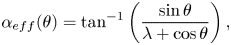 \begin{equation} {{\alpha}_{{eff}}}(\theta) = \tan^{{-}1}\left(\frac{\sin \theta}{\lambda + \cos \theta}\right), \end{equation}
where  $\lambda = {{U}_{{b}}}/ {{{U}}_{{\infty }}}$ is the tip-speed ratio. The tip-speed ratio is shown to govern the amplitude of the periodic variation in effective flow conditions in (1.1) and (1.2). For low and medium tip-speed ratios, typically $\lambda < 4.5$, the effective angle of attack exceeds the blade's critical stall angle twice during the rotation, which can lead to flow separation on the blade surface.
Vertical-axis wind turbine blade kinematics. (a) The free stream velocity  ${{{U}}_{{\infty }}}$ goes from left to right. Indication of the positive direction of the radial force $ {{F}_{{R}}}$, azimuthal force $ {{F}_{{\theta }}}$ and pitching moment at quarter-chord $ {{M}_{{z}}}$. The blade's velocity is equivalent to the rotational frequency $\omega$ times the turbine's radius $R$. Schematic representation of the definition of the blade's effective angle of attack $ {{\alpha }_{{eff}}}$ and velocity $ {{U}_{{eff}}}$ and their temporal evolution (respectively in panels (b) and (c)) as a function of the blade's azimuthal position.

The severity of flow separation events increases for decreasing tip-speed ratios. The tip-speed ratio is considered low when the turbine blade exceeds its static stall angle for longer than 4.5 convective times, corresponding to the minimum amount of time required for a coherent leading-edge vortex to form (Reference DabiriDabiri, 2009; Reference Le Fouest, Deparday and MullenersLe Fouest, Deparday, & Mulleners, 2021; Reference Le Fouest and MullenersLe Fouest & Mulleners, 2022). Vertical-axis wind turbines operating at low tip-speed ratios ( $\lambda \leq 2.5$ when $c/D = 0.2$) undergo deep dynamic stall, which is characterised by the formation, growth and shedding of large-scale coherent vortices (Reference Carr, Mcalister and MccroskeyCarr, Mcalister, & Mccroskey, 1977). The shedding of large-scale vortices is generally followed by a dramatic loss in aerodynamic efficiency and highly unsteady loads that can potentially lead to turbine failure (Reference Corke and ThomasCorke & Thomas, 2015; Reference MccroskeyMccroskey, 1982; Reference Mulleners and RaffelMulleners & Raffel, 2013).
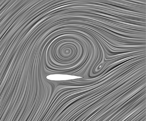
The temporal occurrence and landmark stages characterising dynamic stall on two-dimensional pitching airfoils in a steady free stream flow are well documented (Reference Carr, Mcalister and MccroskeyCarr et al., 1977; Reference Degani, Walker and SmithDegani, Walker, & Smith, 1998; Reference Mulleners and RaffelMulleners & Raffel, 2013) and their load responses can be reasonably well modelled (Reference Ayancik and MullenersAyancik & Mulleners, 2022; Reference Goman and KhrabrovGoman & Khrabrov, 1994; Reference Leishman and BcddoesLeishman & Bcddoes, 1989). For a rotating wind turbine blade, the occurrence of dynamic stall is affected by the circularity of the blade's path in several ways. The dynamic stall vortex is convected downstream along the blade's path after it is shed, extending the blade–vortex interaction compared to a blade pitching in a steady flow. The flow topology is dominated by the extended presence of a dissipating dynamic stall vortex at the overlap between the upwind and downwind halves of the blade rotation when the effective velocity is at its lowest (Figure 1c) (Reference Dave and FranckDave & Franck, 2021; Reference Simão Ferreira, Van Zuijlen, Bijl, Van Bussel, Van Kuik, Ferreira and Van KuikSimão Ferreira et al., 2009). The flow and wake curvature also influence the effective flow acting on a vertical-axis wind turbine blade, leading to virtual camber and incidence effects (Reference Benedict, Lakshminarayan, Pino and ChopraBenedict, Lakshminarayan, Pino, & Chopra, 2016; Reference Migliore, Wolfe and FanucciMigliore, Wolfe, & Fanucci, 1980). The blade crosses the same stream tube twice, leading to repeated blade–wake interactions even for a single-blade configuration (Reference Fujisawa and ShibuyaFujisawa & Shibuya, 2001; Reference ParaschivoiuParaschivoiu, 1988). Typical descriptions of effective flow conditions on a turbine blade, based on (1.1) and (1.2), do not faithfully capture the complexity of the events unfolding during the blade's rotation, even when coupled with an additional induced velocity term (Reference Ayati, Steiros, Miller, Duvvuri and HultmarkAyati, Steiros, Miller, Duvvuri, & Hultmark, 2019; Reference Paraschivoiu and DelclauxParaschivoiu & Delclaux, 1983).
Low-order models, such as the actuator cylinder model, improve the prediction of effective flow conditions and unsteady loads by accounting for the velocity induced to the flow by the presence of a rotating turbine (Reference MadsenMadsen, 1982). The absence of a reliable dynamic stall model for vertical-axis wind turbines limits the validity of low-order models for low to intermediate tip-speed ratios (Reference Dave, Strom, Snortland, Williams, Polagye and FranckDave et al., 2021). The most widely used dynamic stall models were developed for pitching blades operating in a free stream (Reference Goman and KhrabrovGoman & Khrabrov, 1994; Reference Leishman and BcddoesLeishman & Bcddoes, 1989). These models rely on a sound understanding of landmark time scales that govern the development of flow separation, namely the vortex formation time and vortex shedding frequency (Reference Ayancik and MullenersAyancik & Mulleners, 2022). For a vertical-axis wind turbine, the time scales of landmark stall events, such as shear layer roll-up or stall onset, have not yet been characterised. Dynamic stall time scales are crucial parameters in the overall design and modelling of a vertical-axis wind turbine and for more advanced applications such as devising active flow control strategies.
This investigation aims at improving our qualitative and quantitative understanding of the chain of events leading to dynamic stall on a vertical-axis wind turbine blade and the associated time scales. We present time-resolved velocity field and load measurements on a scaled-down H-type Darrieus wind turbine operating in a water channel. A large range of tip-speed ratios is covered to yield a comprehensive characterisation of the occurrence of deep stall on a vertical-axis wind turbine.
2. Experimental materials and methods
The experiments were conducted in a recirculating water channel with a test section of  $0.6\ {\rm m}\ \times\ 0.6\ {\rm m}\ \times\ 3\ {\rm m}$ and a maximum flow velocity of 1 m s
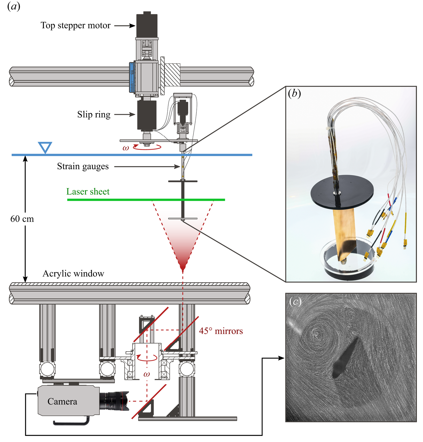
 $^{-1}$. A cross-sectional view of the full experimental apparatus is shown in Figure 2. The main features of the experimental set-up, force and velocity field measurements, and data analysis using proper orthogonal decomposition are summarised here. More details can be found in the supplementary material available at https://doi.org/10.1017/flo.2023.5.
(a) Cross-sectional view of the experimental set-up including the wind turbine model, the light sheet, the rotating mirror system and the high-speed camera for particle image velocimetry. (b) A close-up view of the blade sub-assembly, with installed strain gauges. (c) The camera's field of view indicated by a long exposure image of seeding particles in the flow.
2.1 Experimental set-up
A scaled-down model of a single-bladed H-type Darrieus wind turbine was mounted in the centre of the test section (Figure 2a). The turbine had a variable diameter  $D$ that was kept constant at 30 cm. Here, we used the single-blade configuration to focus on the flow development around the blade in the absence of interference from the wakes of other blades. The blade had a NACA0018 profile with a span of $s=15\ {\rm cm}$ and a chord of $c=6\ {\rm cm}$, yielding a chord-to-diameter ratio of $c/D={0.2}$.
The turbine model was driven by a NEMA 34 stepper motor with a  ${0.05}^\circ$ resolution for the angular position. The rotational frequency was kept constant at 0.89 Hz to maintain a constant chord-based Reynolds number of $ {{{Re}}_{{c}}} = (\rho \omega R c)/\mu = {50\ 000}$, where $\rho$ is the density and $\mu$ the dynamic viscosity of water. To investigate the role of the tip-speed ratio in the occurrence of dynamic stall, we systematically varied the water channel's incoming flow velocity from 0.14 m s $^{-1}$ to 0.70 m s $^{-1}$ to obtain tip-speed ratios ranging from 1.2 to 6.
2.2 Force measurements
The aerodynamic forces acting on the turbine blade were recorded at 1000 Hz for 100 full turbine rotations using strain gauges that were glued onto the shaft (Figure 2b). The forces presented in this paper were the two shear forces applied at the blade's mid-span in the radial  $ {{F}_{{R}}}$ and azimuthal $ {{F}_{{\theta }}}$ direction, and the pitching moment about the blade's quarter-chord $ {{M}_{{1/4}}}$ (Figure 1a). The total force applied to the blade is computed by combining the two shear forces: $ {{F}_{{tot}}} = \sqrt { {{F}_{{R}}}^2 + {{F}_{{\theta }}}^2}$. All force coefficients are non-dimensionalised by the blade chord $c$, the blade span $s$ and the blade velocity $ {{{U}}_{{b}}} = \omega R$ such that:
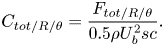 \begin{equation} {{C}_{{tot/R/\theta}}} = \frac{{{F}_{{tot/R/\theta}}}}{0.5\rho {{{U}}_{{b}}}^2 sc}. \end{equation}
The subscripts  $tot, R$ or $\theta$ refer to the total force, the radial or the tangential force component.
From our load measurements, we retrieve an idealised turbine power coefficient. The instantaneous power  $P$ generated by a vertical-axis wind turbine is linearly proportional to the tangential aerodynamic force experienced by the blade:
 \begin{equation} P(\theta) = {{F}_{{\theta}}} \omega R , \end{equation}
where  $\omega$ is the rotational frequency and $R$ is the turbine's radius. This definition of the power is idealised because it does not account for any mechanical or electronic losses that would occur on a wind turbine between the turbine blade torque generation and the generator's output. We can calculate the instantaneous power coefficient by normalising the estimated instantaneously generated power by the power available in the flow:
 \begin{equation} {{C}_{{P}}}(\theta) = \frac{P}{0.5\rho {{{U}}_{{\infty}}}^3 {{A}_{{swept}}}}, \end{equation}
where  $ {{A}_{{swept}}}$ is the turbine's swept area given by the product of the turbine diameter and the blade's span.
2.3 Particle image velocimetry
In addition to the blade load measurements, we conducted time-resolved particle image velocimetry (PIV) in the mid-span cross-sectional plane of the blade with an acquisition frequency of 1000 Hz. With the help of a rotating mirror system that spins with the same frequency as the wind turbine, we were able to keep a field of view of  $2.5c \times 2.5c$ that was centred around the blade (Figure 2c).
The particle images were processed following standard procedures using a multi-grid algorithm (Reference Raffel, Willert, Wereley and KompenhansRaffel, Willert, Wereley, & Kompenhans, 2007). The final window size was  $48\ {\rm pixels}\times 48\ {\rm pixels}$ with an overlap of 75 %. This yielded a grid spacing or physical resolution of $1.7\ {\rm mm} = 0.029c$. A window overlap above 50 % was selected to minimise spatial averaging of the velocity gradients by the interrogation window following Reference Richard, Bosbach, Henning, Raffel, Willert and van der WallRichard et al. (2006), Reference Kindler, Mulleners, Richard, van der Wall and RaffelKindler, Mulleners, Richard, van der Wall, and Raffel (2011). The out-of-plane vorticity component was calculated from the in-plane velocity components using a central difference scheme.
The experimental facility and apparatus were previously described by the authors in Reference Le Fouest and MullenersLe Fouest and Mulleners (2022). More details on the experimental procedure and the turbine model are provided in the supplementary material.
2.4 Proper orthogonal decomposition
The flow development during a full blade rotation is characterised by significant changes in the flow topology and the formation of vortices when dynamic stall occurs. To identify energetically relevant flow features and their time evolution, we apply a proper orthogonal decomposition (POD) of the vorticity field. The POD method was introduced to the field of fluid mechanics to identify coherent structures in turbulent flows (Reference LumleyLumley, 2007). The spatial modes  ${\psi }_{n}$ reveal the dominant and recurring patterns in the data. The corresponding temporal coefficients ${a}_{n}$ indicate the dynamic behaviour of the coherent spatial patterns identified in the modes and can be used to extract the characteristic physical time scales of the problem. As the flow under consideration is vortex dominated, we have opted to decompose the vorticity field instead of the velocity field which was used by Reference Dave and FranckDave and Franck (2023). The vorticity field highlights both the rotational and the strain-dominated regions which are both important to understand dynamic stall development (Reference Menon and MittalMenon & Mittal, 2021). The POD decomposes the vorticity snapshots at time $ {{t}_{{i}}}$ into a sum of orthonormal spatial modes $ {{\boldsymbol {\psi }}_{{n}}}(x, y)$ and their time coefficients $ {{a}_{{n}}}( {{t}_{{i}}})$ such that
 \begin{equation} \boldsymbol{\omega}(x, y, {{t}_{{i}}}) = \sum_{n = 1}^{N}{{a}_{{n}}}({{t}_{{i}}}) {{\psi}_{{n}}}(x, y),\end{equation}
where  $N$ is the total number of snapshots. The POD modes $ {{\psi }_{{n}}}$ form an optimal basis, from which the original system can be reconstructed with the least number of modes compared to any other basis (Reference SirovichSirovich, 1987; Reference Taira, Brunton, Dawson, Rowley, Colonius, McKeon and UkeileyTaira et al., 2017).
In this study, we have used the phase-averaged snapshots of the flow field for the PIV analysis to focus on the dynamics within a rotational cycle and to decrease the computational cost of the POD. The dominant POD modes and large-scale vortical structures are similar with both the time-resolved and phase-averaged data. More information about the phase-averaging procedure are included in the supplementary material. The region of interest for the POD analysis covers the entire overlapping measurement field of view which covers the airfoil and the main flow features on each side.
A key aspect of our study is to compare the dominant flow features shared across varying tip-speed ratios and their relative importance for each case. To this purpose, we have stacked five series of  $200$ phase-averaged vorticity fields $\omega ^{\lambda }(x,y, {{t}_{{i}}})$, with $i=1,\ldots,200,$ corresponding to five tip-speed ratios $\lambda \in [1.2, 1.5, 2, 2.5, 3]$ along the time axis into a single matrix $\varOmega = [\omega ^{\lambda ={1.2}}, \omega ^{\lambda ={1.5}}, \ldots, \omega ^{\lambda ={3}}]^T$ containing $1000$ snapshots. The POD of the combined matrix $\varOmega$ yields the spatial modes $ {{\psi }_{{n}}}(x,y)$, which are common for all cases. The mode coefficient matrix comprises the mode coefficients corresponding to the individual cases $\boldsymbol {A}=[a^{\lambda =1.2}, a^{\lambda =1.5}, \ldots, a^{\lambda =3}]$. The POD eigenvalues $ {{\zeta }_{{n}}}$ indicate the contribution of each mode $n$ to the total energy of the stacked vorticity fields. They are strictly decreasing as POD ranks the modes according to their energy content. With this approach, the vorticity fields for each tip-speed ratio can be reconstructed based on the same set of spatial modes. The temporal contribution of these common structures to individual tip-speed ratios $\lambda$ is given by the corresponding temporal coefficients $ {{a}_{{n}}}^{\lambda }$. A vorticity field for a specific $\lambda = {{\lambda }_{{m}}}$ can be reconstructed as
 \begin{equation} \boldsymbol{\omega}^{\lambda = {{\lambda}_{{m}}}}(x, y, {{t}_{{i}}}) = \sum_{n = 1}^{N}{{a}_{{n}}}^{\lambda = {{\lambda}_{{m}}}}({{t}_{{i}}}){{\psi}_{{n}}}(x,y). \end{equation}
The energy contribution  $ {{\zeta }_{{n}}}^{\lambda = {{\lambda }_{{m}}}}$ of individual spatial modes $ {{\psi }_{{n}}}(x,y)$ in the tip-speed ratio case $\lambda = {{\lambda }_{{m}}}$ is computed from the corresponding time coefficients as
 \begin{equation} {{\zeta}_{{n}}}^{\lambda = {{\lambda}_{{m}}}} = \langle {{a}_{{n}}}^{\lambda = {{\lambda}_{{m}}}},{{a}_{{n}}}^{\lambda = {{\lambda}_{{m}}}}\rangle = \frac{1}{{{N}_{{t}}}} \sum_{i = 1}^{{{N}_{{t}}}} ({{a}_{{n}}}^{\lambda = {{\lambda}_{{m}}}}({{t}_{{i}}}))^2, \end{equation}
where  $ {{N}_{{t}}}=200$ is the number of phase-averaged snapshots of the individual tip-speed cases. The procedure used here is similar to the parametric modal decomposition presented by Reference Coleman, Thomas, Gordeyev and CorkeColeman, Thomas, Gordeyev, and Corke (2019).
3. Results
3.1 Dynamic stall overview
We first present an overview of the development of flow structures and aerodynamic forces experienced by a vertical-axis wind turbine blade undergoing deep dynamic stall. The temporal evolution of the phase-averaged power coefficient for a wind turbine operating at tip-speed ratio  $\lambda = 1.5$ is shown as a polar plot in Figure 3. The interplay between the power coefficient and the flow structures forming around the wind turbine blade is highlighted with phase-average vorticity fields presented throughout the blade's rotation. The total aerodynamic force orientation and relative magnitude are represented by an arrow starting from the blade's quarter-chord.
Polar plot of the temporal evolution of the phase-averaged power coefficient  $ {{C}_{{P}}}$ for a vertical-axis wind turbine operating at tip-speed ratio $\lambda = 1.5$. Phase-averaged normalised vorticity fields are shown throughout the blade's rotation. The total aerodynamic force acting on the blade at the various azimuthal locations is depicted by arrows starting from the blade's quarter-chord. The length of the arrows indicates the relative magnitude of the force. The black circle indicates $ {{C}_{{p}}}=0$. The blue and red regions respectively represent regions where the blade experiences net thrust or net drag.
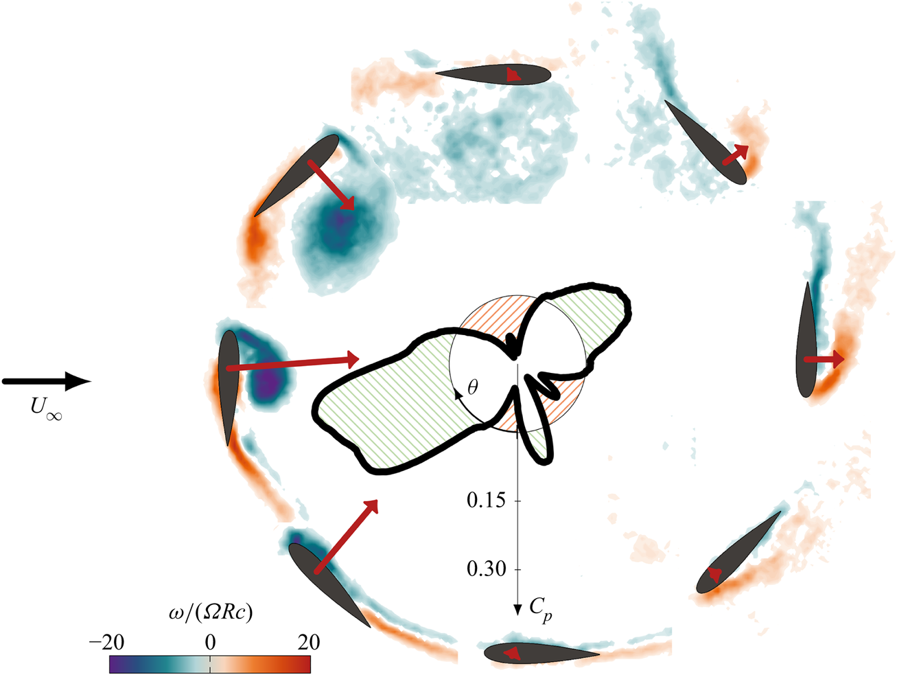
When the blade is facing the wind ( $\theta = {0}^\circ$), the flow is attached and vorticity is only present in the blade's wake. The total force is small but increases rapidly when the blade moves upwind. At $\theta = {33}^\circ$, the blade's effective angle of attack exceeds its critical static stall angle, which was $ {{\alpha }_{{ss}}}={13}^\circ$, and flow reversal emerges on the suction side of the blade. The shear layer rolls up to form a coherent dynamic stall vortex at the leading edge of the blade. The presence of this leading-edge dynamic stall vortex causes the power coefficient to rise from $-0.03$ at $\theta = {0}^\circ$ to its maximum value of 0.32 at $\theta = {77}^\circ$. Thereafter, the dynamic stall vortex continues to grow in size and strength and moves from the leading edge towards the mid-chord position. This migration redirects the aerodynamic force in the radial direction and the power coefficient rapidly drops when the vortex detaches from the blade around $\theta = {114}^\circ$. After lift-off, the stall vortex is convected downstream along the blade's path, dissipates and breaks apart into smaller scale structures. The massive flow separation leads to a drop in the total forces acting on the blade and a collapse of the power production. The power coefficient remains around its minimum value of $-0.14$ between $\theta = {150}^\circ$ and $\theta = {180}^\circ$. During the downwind half of the blade's rotation ( ${180}^\circ \leq \theta < {360}^\circ$), there is a reversal between the suction and pressure sides of the blade. A second counter-rotating leading-edge vortex now forms on the extrados of the blade's circular path ( $\theta = {240}^\circ$). This vortex is less coherent and less strong than that formed during the upwind. It still yields a local maximum in the power coefficient around 0.1. The second leading edge vortex does not remain bound to the blade for long and before we reach $\theta = {270}^\circ$, a layer of negative vorticity is entrained between the vortex and the blade surface. The lift-off of the second leading edge vortex leads again to a drop in the power coefficient below 0. The power coefficient reaches a local minimum of $-0.07$ at $\theta = {329}^\circ$. This phase position corresponds to the moment when the blade's angle of attack returns below its critical stall angle and flow reattachment is initiated.
Dynamic stall plays a central role in the temporal evolution of the power coefficient for vertical-axis wind turbines operating at low tip-speed ratios. For all cases with  $\lambda \leq 2.4$ in our configuration, we observe a succession of six characteristic stages, including attached flow, shear layer growth, upwind vortex formation, upwind stall, downwind stall and flow reattachment. The wind turbine's performance varies significantly from one stage to the next. Here, we focus on the characterisation of the temporal development of the flow structures during the full dynamic stall life cycle, their influence on the unsteady load response and turbine power production, and changes in the life cycle as a function of the tip-speed ratio.
3.2 Proper orthogonal decomposition and modal analysis
We use the POD of the vorticity field to identify the energetically dominant spatial modes that characterise the flow around our vertical-axis wind turbine blade. The POD time coefficients associated with the dominant spatial modes are examined to identify the characteristic dynamic stall time scales. A single set of spatial eigenmodes is extracted from the ensemble of phase-averaged vorticity fields measured at different tip-speed ratios following the procedure described in § 2.4.
The eigenvalues  $ {{\zeta }_{{n}}}^{\lambda }$ associated with the first ten spatial POD modes for different tip-speed ratios are presented in Figure 4. The tip-speed-ratio-specific eigenvalues are calculated according to (2.6) and represent the energy contribution of the individual spatial modes in the vorticity field reconstruction for the specific tip-speed ratio. The eigenvalues are normalised by the sum of the tip-speed-ratio-specific eigenvalues. Overall, the energy contribution of the modes decreases rapidly with increasing mode number and the first three modes represent more than 70 % of the energy for all tip-speed ratios. Analysing flow structures with POD requires striking a balance between conciseness and completeness. Selecting too few modes means one might ignore a too large energetic portion of the flow, while selecting too many sacrifices the benefits of a low-order analysis. Here, we focus on the first three spatial modes to analyse the temporal development of dominant flow features.
Normalised eigenvalues associated with the first ten spatial POD modes for different tip-speed ratios calculated according to (2.6).

The first three spatial POD modes are presented in Figure 5. The corresponding time coefficients are shown for tip-speed ratios  $\lambda = 1.2, 1.5, 2.0, 2.5$ and $3.0$. The time coefficients $ {{a}_{{n}}}$ are normalised by the eigenvalues obtained from the stacked flow field POD (§ 2.4). The first spatial mode is characterised by the presence of a large dynamic stall vortex with a vortex centre located at mid-chord and half-chord length above the blade's surface. Note that the modes are presented in the blade's frame of reference. Everything that is above the blade corresponds to what happens on the intrados of the blade's rotational trajectory. The temporal evolution of the corresponding time coefficient $ {{a}_{{1}}}$ shows a distinctive peak when the upwind dynamic stall vortex is prominent. The amplitude of the peak increases with decreasing tip-speed ratio. The increase in amplitude highlights a more dominant large-scale vortex for decreasing tip-speed ratio. At lower tip-speed ratios, the maximum effective angle of attack increases (Figure 1) and the strength of the dynamic stall vortex increases (Reference Le Fouest and MullenersLe Fouest & Mulleners, 2022). The first POD mode and the corresponding time coefficient can be used to characterise the time scales related to the formation of the upwind dynamic stall vortex.
(a.i)–(c.i) First three spatial POD modes and (a.ii)–(c.ii) the evolution of the corresponding time coefficients for tip-speed ratios  $\lambda = 1.2, 1.5, 2.0, 2.5$ and $3.0$.
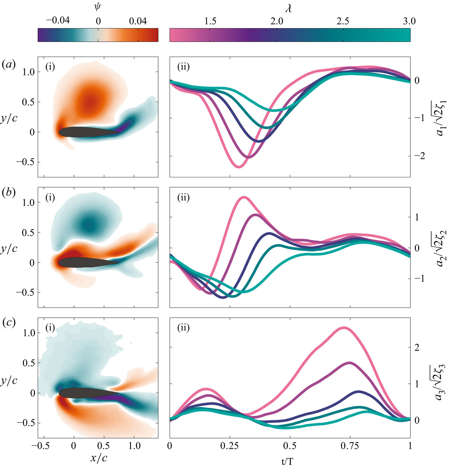
The interpretation of the second spatial POD mode is more intricate than that of the first one, as it seems to combine two consecutive events that occur in the flow. The time coefficient  $ {{a}_{{2}}}$ is negative at the start of the upwind and initially decreases for all cases ( $0 \leq t/T < 0.25$). During this time period, flow reversal is first observed on the suction side of the turbine blade or the intrados of the blade's rotational trajectory. Once the blade exceeds its critical stall angle, the time coefficient $ {{a}_{{2}}}$ starts to increase, becomes positive and peaks at the occurrence of vortex lift-off. The increase in $ {{a}_{{2}}}$ can be interpreted as the transition from a strong accumulation of negative vorticity near the surface during flow reversal to the growth of a large vortex that entrains positive vorticity near the surface that leads to separation of the main upwind stall vortex. The positive peak of the second mode coefficient occurs at the same time as the negative peak of the first mode coefficient. The first two modes do not form a classical mode pair, where energy is transferred from one to the other, they rather reinforce each other. The second POD mode and the corresponding time coefficient can be used to characterise the transition from the accumulation of vorticity and growth of the shear layer to the roll-up of the shear layer into a large-scale upwind dynamic stall vortex.
The third spatial POD mode does not display the presence of a coherent flow structure but rather a state of massively separated flow. The corresponding time coefficient  $ {{a}_{{3}}}$ significantly increases immediately after the separation of the upwind stall vortex, which corresponds to the moment when the amplitude of the first time coefficient $ {{a}_{{1}}}$ decreases. The third spatial mode represents the fully separated flow following vortex detachment. The severity of the post-stall conditions increases with decreasing tip-speed ratio. Low tip-speed ratio cases are characterised by the formation of a stronger dynamic stall vortex than intermediate and high tip-speed ratio cases and they experience more pronounced deep stall events. The absence of a coherent flow structure in the third spatial mode explains the asymmetry in power production between the upwind and downwind halves of the rotation presented exemplarily in Figure 3. During upwind, a torque-producing coherent leading-edge vortex is formed. During downwind, the flow is massively separated and the loads are characterised by drag excursions.
The time coefficients of the first three POD modes will be used next to identify the timing of the different dynamic stall stages. The fourth POD mode, which plays a more prominent role than the third mode for higher tip-speed ratios where stall is less prominent, did not provide additional information for the identification of the stall stages. It is included for reference in the supplementary material.
3.3 Identification of dynamic stall stages using POD time coefficients
The trajectories in the feature space spanned by the POD time coefficients corresponding to the three dominant modes are shown in Figure 6(a) for tip-speed ratio cases  $\lambda = 1.2, 1.5, 2.0, 2.5$ and $3.0$. The trajectory corresponding to the tip-speed ratio $\lambda = 1.5$ is colour-coded and used as an example to demonstrate our approach to identifying the timing of the various stages in the flow development. The feature space representation highlights the interplay between the time coefficients. We analyse the points of inflexion of the trajectory. A change in the relative importance of the time coefficient creates an inflexion point on the trajectory in the feature space and relates to key events in the flow development. The inflexion points were systematically compared to the phase-averaged flow fields to determine their physical significance. The results presented here are manually extracted and subject to the authors’ discretion. The inflection points were found by inspecting the three-dimensional curves from various orientations. Not all of them are visible in the two-dimensional projection depicted in Figure 6(a). Additional projections are included in the supplementary material.
(a) Time coefficient parametric curve obtained from the stacked vorticity field POD (§ 2.4). (b) Phase map of the characteristic dynamic stall stages experienced by the wind turbine blade operating at tip-speed ratio  $\lambda = 1.5$. The stages are: attached flow (pink), shear layer growth (light green), vortex formation (green), upwind stall (purple), downwind stall (blue) and flow reattachment (light blue). (c) Selected snapshots of the flow topology representing the characteristic stall stages obtained by the line integral convolution method. (d) Duration and timing of the dynamic stall stages for tip-speed ratio cases $\lambda = 1.2, 1.5, 2.0, 2.5$ and $3.0$.

We identify the timing and duration of six landmark stages: attached flow (pink), upwind shear layer growth stage (light green), upwind vortex formation stage (green), upwind stalled stage (purple), downwind stalled stage (blue) and flow reattachment (light blue). A phase map for the six stages is shown for  $\lambda = 1.5$ in Figure 6(b). Visualisations of the flow topology characteristic of the individual stages are obtained by applying the line integral convolution (LIC) method (Reference Cabral and LeedomCabral & Leedom, 1993) to phase averaged flow field snapshots (Figure 6c). The timing and duration of the dynamic stall stages are summarised in Figure 6(d).
The same six stages occur for all tip-speed ratios, but the timing and duration of these stages vary. The flow is attached when the blade enters the upwind part of the rotation for all cases. First signs of stall development occur when the blade exceeds its critical stall angle, which happens later in the cycle for higher tip-speed ratios (Figure 1b). Within less than a quarter of a rotation, a coherent upwind stall vortex has formed, which continues to grow in the chord-wise and chord-normal direction until the vortex lifts off and opposite-signed vorticity is entrained between the vortex and the blade's surface. The entrainment of secondary vorticity ultimately leads to the detachment of the stall vortex and the onset of upwind dynamic stall. This process is similar to the vortex-induced separation observed on two-dimensional pitching and plunging airfoils (Reference Doligalski and SmithDoligalski & Smith, 1994; Reference Mulleners and RaffelMulleners & Raffel, 2012; Reference Rival, Kriegseis, Schaub, Widmann and TropeaRival, Kriegseis, Schaub, Widmann, & Tropea, 2014).
The upwind dynamic stall onset is identified in the POD feature space in Figure 6(a) as the local maximum of  $ {{a}_{{2}}}$ and the minimum of $ {{a}_{{1}}}$. The time interval between the moment when the blade exceeds its critical stall angle and the onset of stall is defined as the upwind stall development. We divide the upwind stall development into two parts in analogy with the flow development observed on pitching airfoils (Reference Deparday and MullenersDeparday & Mulleners, 2019; Reference Mulleners and RaffelMulleners & Raffel, 2013). The first part is characterised by the accumulation of bound vorticity and the thickening of the surface shear layer. We call this stage the shear layer growth stage. The shear layer growth stage (light green) takes up a larger portion of the cycle when the tip-speed ratio increases (Figure 6d). A kink in the feature space at the minimum of $ {{a}_{{2}}}$ and a local extremum of $ {{a}_{{1}}}$ marks the start of the roll-up of the shear layer into a coherent dynamic stall vortex. This second part of the upwind stall development is characterised by the growth of the upwind dynamic stall vortex and is called the upwind vortex formation stage. The vortex formation stage (green) occupies approximately the same portion of the cycle for all tip-speed ratios but ends earlier in the cycle for lower tip-speed ratios (Figure 6d). Stall onset marks the end of the vortex formation stage and the start of the upwind stalled stage.
The next transition is marked by the switch of the leading edge stagnation point from the intrados of the blade path to the extrados, which corresponds respectively to the top and the bottom side of the blade in the snapshots presented in Figure 5(a.i)–(c.i). This transition is identified in the POD feature space as an inflexion point in the gradient of  $ {{a}_{{3}}}$ and occurs at approximately the same point in the cycle (Figure 6d). As the blade enters the downwind half of the rotation, the fully separated flow has no time to reattach to the blade even though the angle of attack is theoretically at ${0}^\circ$ when $\theta = {180}^\circ$. Furthermore, the blade's angle of attack varies more rapidly in the first part of the downwind than during the upwind. There is insufficient time for a clear shear layer growth and vortex formation stage during the downwind, so we only consider an overall downwind stalled stage (Reference Le Fouest and MullenersLe Fouest & Mulleners, 2022). The end of the downwind stalled stage is marked by the maximum value of $ {{a}_{{3}}}$ and it is followed by the flow reattachment stage. The flow reattaches to the blade for all cases in the last quarter of the turbine's rotation.
The characteristic upwind dynamic stall delay is the combined duration of the shear layer growth and the vortex formation stage. Based on previous work, we expect that the duration of the stall delay expressed in convective time scales becomes independent of the kinematics for larger reduced frequencies (Reference Ayancik and MullenersAyancik & Mulleners, 2022; Reference Le Fouest, Deparday and MullenersLe Fouest et al., 2021). Generally, the non-dimensional convective time is obtained by dividing the physical time by  $c/{U}$, with ${U}$ a constant characteristic velocity. Here, the effective flow velocity experienced by the blade changes constantly and instead of using the blade velocity or the free stream velocity to obtain a non-dimensional convective time, we opt here to take the constantly varying effective flow velocity into account and calculate the convective time perceived by the turbine blade using
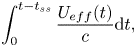 \begin{equation} \int_{0}^{t - {{t}_{{ss}}}} \frac{{{{U}}_{{eff}}}(t)}{c} \mathrm{d} t, \end{equation}
where  $ {{U}_{{eff}}}$ is the effective flow velocity obtained from the vectorial combination of the blade velocity and the incoming flow velocity (Figure 1).
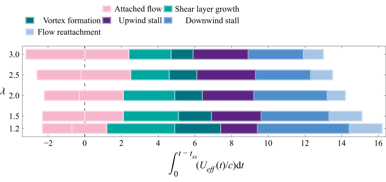
The temporal occurrence of dynamic stall stages scaled with the convective time is presented in Figure 7. Note that we subtract the time at which the static stall angle is exceeded  $ {{t}_{{ss}}}$ to realign subsequent stall events, in accordance with results presented by Reference Buchner, Soria, Honnery and SmitsBuchner et al. (2018). When we express the upwind stall delay (light green + green) in terms of convective times, the stall delay does not depend on the tip-speed ratio and converges to approximately 4.5 convective times, which matches standard vortex formation times found in the literature (Reference DabiriDabiri, 2009; Reference Dunne, Schmid and McKeonDunne, Schmid, & McKeon, 2016; Reference Gharib, Rambod and ShariffGharib, Rambod, & Shariff, 1998; Reference Kiefer, Brunner, Hansen and HultmarkKiefer, Brunner, Hansen, & Hultmark, 2022). The combination of the upwind and downwind stalled stages also reaches similar values for all tip-speed ratios, although the distribution between the two stages varies. The flow reattachment time scale decreases slightly for increasing tip-speed ratios. This trend may be due to the discrepancy between the effective flow velocity calculated using (1.1) and the actual effective flow velocity acting on the turbine blade in the downwind half of the turbine rotation. Equation (1.1) neglects any influence of the induced velocity from shed vorticity, which is abundant in the downwind half of the turbine's rotation. Overall, the convective time offers a promising scaling option for dynamic stall time scales on vertical axis turbines. Further work can aim at modelling the influence of vorticity induced velocity to improve the scaling and implement universal time scales into dynamic stall modelling and control strategies for vertical-axis wind turbines.
Duration and timing of the dynamic stall stages for tip-speed ratio cases  $\lambda = 1.2, 1.5, 2.0, 2.5$ and $3.0$ in terms of the convective time. The stages are: attached flow (pink), shear layer growth (light green), vortex formation (green), upwind stall (purple), downwind stall (blue) and flow reattachment (light blue).
3.4 Identification of dynamic stall stages using the aerodynamic loads
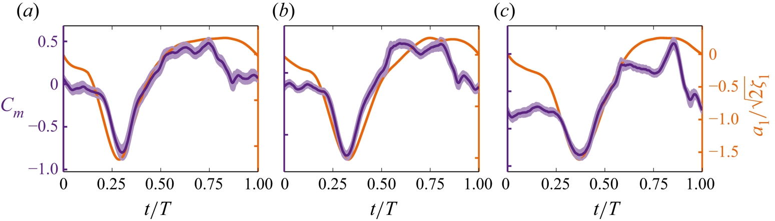
We cannot rely on optical flow measurements if we want to achieve real-time active flow control on a wind turbine blade. The processing time of the flow measurement around the blade, capturing vortex formation or incoming gusts, for instance, is prohibitive to actuate a response in time. Finding patterns in the readily available aerodynamic loads that indicate the occurrence of stall stages is desirable. This feasibility of replacing the time series of the POD coefficients with a load measurement time series was inspired by the similarity between some features in the POD time coefficients and the temporal development of the aerodynamic loads. In Figure 8, we compare the temporal evolution of the time coefficient  $ {{a}_{{1}}}$ corresponding to the first POD mode and the phase-averaged pitching moment coefficient for tip-speed ratios $\lambda = 1.2, 1.5, 2.0$. The general shape of the two curves is in close agreement. The timing of the distinctive peak displayed by the time coefficient $ {{a}_{{1}}}$ perfectly matches the timing of the negative pitching moment peak. The pitching moment is highly sensitive to changes in the formation of the large-scale upwind dynamic stall vortex, which is characterised by the mode coefficient $ {{a}_{{1}}}$. This further confirms our interpretation of the first POD mode and motivates us to extract the timing and duration of the dynamic stall stages based solely on the aerodynamic loads.
Comparison of the temporal evolution of the first POD mode time coefficient  $ {{a}_{{1}}}$ and the phase-averaged pitching moment coefficient for tip-speed ratio cases $\lambda = 1.2, 1.5, 2.0$.
We analyse the dynamic stall time scales based on the development of the unsteady loads experienced by the wind turbine blade using a similar approach as for the POD time coefficients. Our new feature space is built using the azimuthal force, radial force and pitching moment coefficients, and we analyse the measured trajectories in Figure 9(a) for 19 tip-speed ratio cases with  $\lambda \in [1.2\unicode{x2013}3.0]$. The trajectory corresponding to the tip-speed ratio $\lambda = 1.5$ is colour-coded and used as an example to demonstrate the automated identification of the dynamic stall stages from the unsteady loads. Automated identification increases the robustness and the potential of using unsteady loads as the input for active flow control laws. The points of inflexion formed by the unsteady load trajectories are not as clearly defined as those in the POD time coefficient trajectory shown in Figure 5(a), but we are able to identify five extrema that are systematically featured in the temporal development of the aerodynamic loads and that can be directly related to the changes in the dynamic stall life cycle. These extrema were identified by closely analysing the interplay between flow structures developing around the turbine blade and abrupt changes in the load response.
(a) Unsteady force parametric curve for tip-speed ratios  $\lambda \in [1.2\unicode{x2013}3.0]$. The inset shows the phase map of the characteristic dynamic stall stages experienced by the wind turbine blade operating at tip-speed ratio $\lambda = 1.5$. The stages are: attached flow and shear layer growth (light green), vortex formation (green), upwind stall (purple), downwind stall (blue) and flow reattachment (light blue). (b) Duration and timing of the dynamic stall stages retrieved from the unsteady loads for tip-speed ratio $\lambda \in [1.2\unicode{x2013}3.0]$. Temporal evolution of phase-averaged unsteady (c) tangential load coefficient $ {{C}_{{\theta }}}$, (d) pitching moment coefficient $ {{C}_{{M}}}$, (e) radial force coefficient $ {{C}_{{R}}}$ for tip-speed ratios $\lambda \in [1.2\unicode{x2013}3.0]$. Selected snapshots of the flow topology representing the characteristic stall stages are repeated as reminders.

The first extremum we identified is the tangential force minimum occurring shortly after the blade enters the upwind half of its rotation ( $0 \leq t/T < 0.5$) (Figure 9b). This time instant is followed by a strong increase in torque production, which corresponds to the shear-layer growth stage (Figure 3, $\theta = {45}^\circ$). The end of the shear-layer growth stage coincides with the tangential force maximum occurring around $t/T = 0.25$. The vortex formation stage is characterised by the convection of the upwind dynamic stall vortex from the leading edge towards the mid-chord position, causing a significant excursion of the pitching moment coefficient from just below 0 to its minimum value $ {{C}_{{M,min}}}$ (Figure 9c). The pitching moment minimum coincides with vortex separation and the beginning of the upwind stalled stage. Vortex separation is followed by a significant loss in radial force that decreases until approximately $t/T = 0.6$, reaching a plateau that corresponds to the downwind stalled stage. The transition from a sharp decrease to a plateau is identified using the function findchangepts in MATLAB. Lastly, the pitching moment coefficient reached a local maximum before returning to its initial value during the flow reattachment stage. These extrema are used to identify the landmark dynamic stall stages for all tip-speed ratio cases $\lambda \in [1.2\unicode{x2013}3.0]$.
A phase map showing the temporal occurrence of dynamic stall stages identified using unsteady loads is shown as an inset in Figure 9(a) for  $\lambda = 1.5$. The stages we identify from loads are the same as those identified using the time coefficient of the vorticity field POD with one exception: the attached flow stage. There is no clear indication of an attached stage in the unsteady load response. The blade experiences an immediate load response to the increase of the effective angle of attack at the beginning of the blade's rotation, but the appearance of flow reversal and shear-layer growth is delayed to higher angles of attack. The first stage (light green) shown in Figure 9(e) thus combines the attached flow stage and the shear layer growth stage. The timing and duration of the following stages match those computed with the POD time coefficients. These findings suggest that the aerodynamic loads contain sufficient information to identify whether a wind turbine blade is undergoing dynamic stall and in which stage is the flow development.
3.5 Stage-wise comparison of both identification methods
A direct comparison of both stage identification methods is desirable to assess the potential of unsteady loads to capture the time scales of flow development for analytical or control purposes. To allow for a direct comparison between the stages computed from the aerodynamic loads and those obtained using the POD time coefficients, we calculated the work done by the total aerodynamic force in each stage for both methods. The work done by the total aerodynamic force over a given stage is calculated by
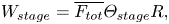 \begin{equation} {{W}_{{stage}}} = \overline{{{F}_{{tot}}}} {{\varTheta}_{{stage}}} R, \end{equation}
where  $\overline { {{F}_{{tot}}}}$ is the mean total aerodynamic force experienced by the turbine blade over that stage and $ {{\varTheta }_{{stage}}}$ is the angular distance covered by the blade throughout the stage. This metric allows a pertinent comparison between the two stage identification methods because it accounts for both the duration of the stage and the magnitude of the loads experienced by the turbine blade during that stage. A small error in the time scale of a given stage is enhanced if the stage is related to significant unsteady loads. Alternatively, we could have chosen the blade's time-averaged power production over each stage as a metric, but we preferred the work done by the total force because it accounts for both the radial and tangential force components and has a high signal-to-noise ratio, even for high tip-speed ratio cases when the force magnitude is lower.
The stage-wise contributions to the work completed by the aerodynamic force are compared in Figure 10 for stages identified using either the aerodynamic loads or the POD time coefficients for tip-speed ratios  $\lambda = [1.2, 1.5, 2.0, 2.5\ \mathrm {and}\ 3.0]$. To facilitate the comparison, the work completed in each stage $ {{W}_{{stage}}}$ is normalised by the total work completed by the aerodynamic force throughout the blade's rotation $ {{W}_{{total}}} = \overline { {{F}_{{tot}}}} 2 {\rm \pi}R$.
Stage-wise contribution to the total work completed by the total aerodynamic force throughout the blade's rotation. The stage contributions are compared for stages identified either by using aerodynamic loads (dark contours) or by using POD time coefficients (light contours) for tip-speed ratios  $\lambda = [1.2, 1.5, 2.0, 2.5\ \textrm {and}\ 3.0]$. The stages are: attached flow (pink), shear layer growth (light green), vortex formation (green), upwind stall (purple), downwind stall (blue) and flow reattachment (light blue).
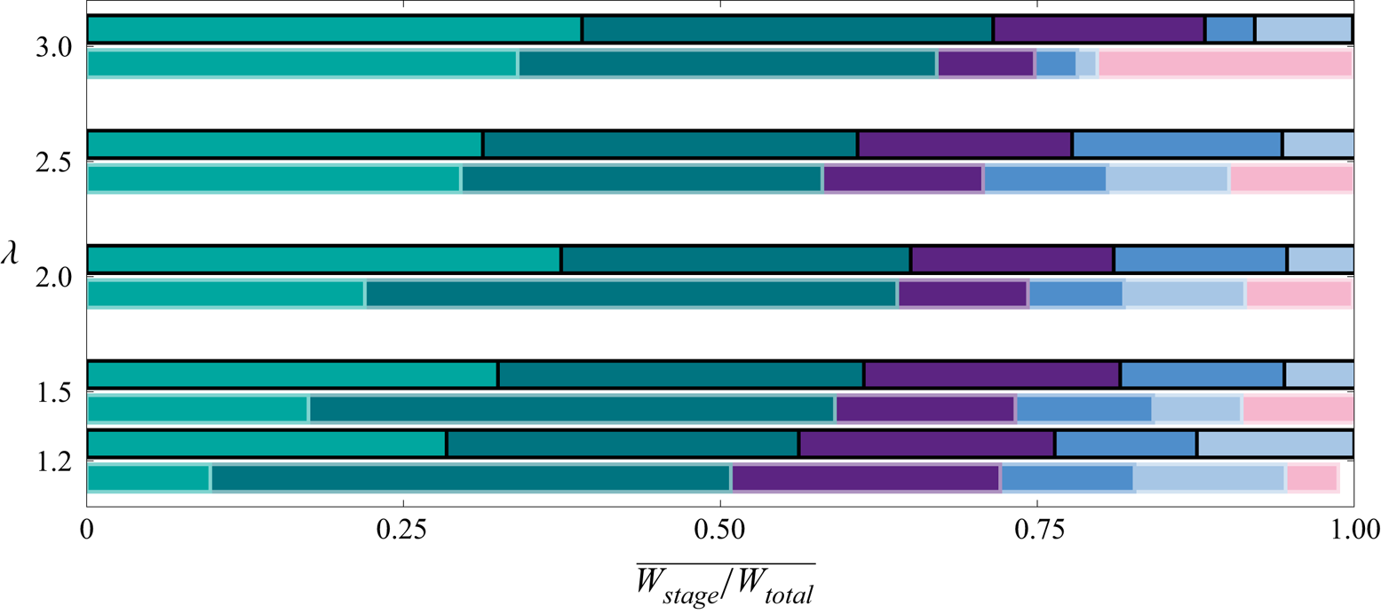
Overall, most of the aerodynamic work is completed during the shear layer growth (light green) and the vortex formation stage (green). These stages are associated with the accumulation of vorticity close to the blade's surface, which creates significant suction over approximately one quarter of the turbine's rotation. This trend is verified for both stage identification methods at all tip-speed ratios. The combined contribution of the shear layer growth and the vortex formation stage is nearly independent of tip-speed ratio and reaches  $0.6$ for all cases. Both stage identification methods show excellent agreement. The aerodynamic loads do not allow for a clear identification of the attached flow stage. Instead, the attached flow stage is distributed across the flow reattachment and the shear layer growth stages. The work contribution of the attached flow stage is limited across tip-speed ratios. The accurate capture of key time scales, such as the vortex formation time, is a satisfactory and promising result for the use of aerodynamic loads as a tool to identify flow development time scales and implement closed-loop control strategies.
4. Conclusion
We collected time-resolved velocity field and unsteady load measurements on a vertical-axis wind turbine operating at low tip-speed ratios  $\lambda \in [1.2\unicode{x2013}3.0]$ to characterise the chain of events that leads to dynamic stall and to quantify the influence of the turbine operation conditions on the duration of the individual stages of the flow development. The dominant flow features and their time scales were first analysed using a proper orthogonal decomposition of the stacked vorticity fields from different tip-speed ratio conditions. This procedure is known as a parametric modal decomposition and yields a single set of representative spatial modes and tip-speed-ratio-specific temporal coefficients and eigenvalues that can be directly compared to characterise the influence of the tip-speed ratio on the temporal development of the dominant spatial flow features.
Based on the POD time coefficients of the three most energetic modes, we were able to identify the timing and duration of six landmark dynamic stall stages: the attached flow, shear layer growth, vortex formation, upwind stall, downwind stall and flow reattachment stage. The duration of the attached flow stage increases with increasing tip-speed ratio as the blade exceeds its critical stall angle later for higher tip-speed ratios. The combined duration of the shear layer growth and vortex formation stages represent the characteristic dynamic stall delay. This dynamic stall delay is independent of tip-speed ratio for our experimental conditions and reaches a constant non-dimensional value of  $4.5$ convective times, which corresponds to the typical dynamic stall delays found on non-rotating pitching and plunging airfoils at comparable reduced frequencies. The upwind and downwind stall stages shorten with increasing tip-speed ratio as the blade spends less time at angles of attack beyond the critical stall angle. Flow reattachment starts once the blade returns below its critical angle and full reattachment is reached within three to four convective times for all cases studied. The dynamic stall stages were also identified based solely on the measured aerodynamic loads. The timing of the dynamic stall stages based on the loads agrees well with the timing based on the time coefficients of the first three modes of the POD of the vorticity field.
Our findings demonstrate that aerodynamic loads are suitable for analysing the time scales of flow development on a vertical-axis wind turbine blade and can be used for flow control applications. However, a control strategy should not necessarily aim at avoiding the onset of dynamic stall as the work completed by the aerodynamic forces during the upwind dynamic stall delay represents approximately 60 % of the total work completed throughout the turbine's rotation. Future work should focus on careful management of the dynamic stall vortex formation and shedding to exploit the work done by the vortex but avoid potential negative ramifications related to its shedding.
Supplementary material
Supplementary material is available at https://doi.org/10.1017/flo.2023.5. The data used in this work will be made available upon request.
Funding statement
Support from the Swiss national science foundation under grant number PYAPP2_173652 is gratefully acknowledged.
Declaration of interests
The authors declare no conflict of interest.


 Open access