2. HORIZONTAL RESOLUTION

Although our main aim is to estimate the error in ice thickness of a DEM, the horizontal resolution of the DEM provides an indication of its quality and thus deserves some attention. We start by noting that both the density of ice-thickness data and the horizontal resolution at each data point contribute to the horizontal resolution of the DEM, although the grid size acts as a lower bound of the horizontal resolution.

As discussed in Paper I, the horizontal resolution of GPR data along profiles depends on whether the radargrams have been migrated or not. For non-migrated data, the horizontal resolution depends on the ice thickness, while for migrated data it does not. However, 2-D migration only corrects the data along the profiling direction, so the resolution in the direction perpendicular to the profile is unaffected by migration. Moreover, in the case of GPR there is a high data density along the profiles, while the zones between radar profiles, often large, are devoid of data. Consequently, the horizontal resolution of the ice-thickness DEM will not be uniform. It will be limited by the spacing between radar traces, by the spacing between radar profiles, by the depth-dependent Fresnel radius (non-migrated profiles) or by λ/2 (migrated profiles, with λ the wavelength of the central frequency of the radar), and by the grid size of the DEM. Following Welch and others’ (Reference Welch, Pfeffer, Harper and Humphrey1998) arguments, even if all the field and processing techniques are properly applied, the maximum horizontal resolution of the DEM will be of λ/2 × λ/2.

3. DATA ERROR

Following Paper I, we consider errors in ice-thickness data, whatever their source is (see classification below), as made up of two components: the error in the value of ice thickness ( $\varepsilon _{H_i} $ ), and the error in thickness due to the uncertainty in horizontal positioning of the datum ( $\varepsilon _{Hxy_i} $ ). Since $\varepsilon _{H_i} $ and $\varepsilon _{Hxy_i} $ are independent of each other, the error in thickness at a given data point is obtained by

(1) $$\varepsilon _{H{\rm data}_i} = \sqrt {\varepsilon _{H_i} ^2 + \varepsilon _{Hxy_i} ^2}. $$

Here, we classify ice-thickness sources for DEM generation into three types with differing error components as follows:

1. (1) ‘Direct’ ice-thickness measurements.

2. (2) Ice-boundary points with known zero ice thickness (e.g. front of land-terminating glaciers or contact of the glacier with its sidewalls).

3. (3) Indirect estimates of ice thickness at zones without direct ice-thickness measurements. We refer to these as ‘synthetic’ data.

We now separately analyse both error components for each ice-thickness-data type.

3.2. Positioning-related ice-thickness error

In Paper I we presented a method to estimate, for GPR measurements, the positioning-related ice-thickness error, $\varepsilon _{Hxy_i} $ , from estimates of the uncertainty in position, ε _xyi . The same procedure can be followed to estimate $\varepsilon _{Hxy_i} $ from other ice-thickness data sources, such as seismic or gravity measurements. The uncertainty in the position ε _xyi of the boundary data deserves particular attention, and is discussed in the following subsection.

In the case of using synthetic ice-thickness data, uncertainty in position,ε _xyi , will depend on the theoretical assumptions made to generate them. For instance, if the estimates depend on the distance to the nearest measurements or to the ice-mass boundary, they will also be affected by the uncertainty in position inherent to these nearest measurements or ice-mass boundary.

Once the uncertainty in position ε _xyi is known, we estimate the positioning-related ice-thickness error as the maximum discrepancy found (absolute value) between the value at the data point and the neighbouring values within a circle of radius ε _xyi , using a DEM of ice thickness. The smoothing effect introduced by the DEM is compensated by the use of the maximum value.

3.2.1. Boundary-positioning error

The ice-mass boundary can include zero and non-zero ice-thickness data. We consider that the zero thickness assigned to boundaries separating ice and ground is free from error in the value of ice thickness, $\varepsilon _{H_i} $ , provided that we take into account, separately, the positioning-related ice-thickness error, $\varepsilon _{Hxy_i} $ . However, at boundary points with non-zero ice-thickness, such as calving fronts, ice divides or artificial sections introduced in the ice to limit the modelling to a particular area, we take into account both the error in the value of ice thickness and the positioning-related ice-thickness error.

In the case of having detailed information on the uncertainty in a certain boundary delineation (e.g. Bernard and others, Reference Bernard2014), the estimate of $\varepsilon _{Hxy_i} $ can be applied at the boundary on a point-by-point basis, using the individual ε _xyi for each boundary point. However, for ice boundaries in which a rough statistical estimate of the error in area is available, we propose to uniformly distribute the uncertainty in area, assigning a common uncertainty to all the boundary points, as shown in Figure 2. It is customary to characterize the uncertainty in boundary position in such cases as a fraction of area, p, of the total area, A (so pA represents the uncertainty in area, and p/100 represents the percentage of error in area) (e.g. Bolch and others, Reference Bolch, Menounos and Wheate2010; Gjermundsen and others, Reference Gjermundsen2011; Nuth and others, Reference Nuth2013; Paul and others, Reference Paul2013; Pfeffer and others, Reference Pfeffer2014).

Fig. 2.

The external polygon represents an ice boundary with area A. The uncertainty in area is assumed to be characterized by means of a fraction p of its total area. The width of the blue-coloured internal band, ε _xy , is chosen so that the area of the band equals pA. This width is used as $\varepsilon _{xy_i} $ for the boundary points.

To estimate the corresponding horizontal uncertainty (ε _xy in Fig. 2) we use the Straight Skeleton routine of the Computational Geometry Algorithms Library (CGAL) version 4.6, http://www.cgal.org/, distributed under the GPL/LGPL open source license. We obtain the horizontal uncertainty $\varepsilon _{xy_i} $ to be applied to every boundary point by letting the width of the blue-coloured internal band grow until its area reaches the total error in area, pA.

4. ICE-THICKNESS INTERPOLATION ERROR

The construction of ice-thickness DEMs involves the interpolation of ice-thickness data to a regular grid. This operation introduces an interpolation error, which will depend on the quantity and distribution of the field data available. The interpolation error at each grid point k will be characterized as $\varepsilon _{H{\rm int}_k} $ . In this study we assume that any extrapolation is avoided. We also assume that the interpolation method used is of weighted-average type (e.g. kriging, splines or inverse distance weighting), because these weights will be used to propagate the errors from the data points to the grid points. In cases using other types of interpolation, such as the approach based on completing the sparse GPR data using mass conservation (e.g. Farinotti and others, Reference Farinotti, Huss, Bauder, Funk and Truffer2009a, Reference Farinotti, Huss, Bauder and Funkb, Reference Farinotti, King, Albrecht, Huss and Gudmundsson2014; Morlighem and others, Reference Morlighem2011, Reference Morlighem2013) or other techniques (e.g. Binder and others, Reference Binder2009; Herzfeld and others, Reference Herzfeld, Wallin, Leuschen and Plummer2011), some parts of our error study should be adapted accordingly.

Different approaches have been followed in the literature to infer the interpolation error. In the case of kriging interpolation, it is well known that the kriging variance underestimates the interpolation error (e.g. Journel, Reference Journel1986; Cressie, Reference Cressie1993, p. 127; Chainey and Stuart, Reference Chainey, Stuart and Carver1998; den Hertog and others, Reference den Hertog, Kleijnen and Siem2006; Rotschky and others, Reference Rotschky2007), although it has been used in glaciology to evaluate the accuracy of the interpolated values (e.g. Bamber and others, Reference Bamber, Layberry and Gogineni2001). Some authors evaluate the uncertainties by comparing the DEMs resulting from different subsets of GPR data (e.g. Fischer, Reference Fischer2009), or bootstrapping methods (e.g. den Hertog and others, Reference den Hertog, Kleijnen and Siem2006; Bamber and others, Reference Bamber2013). Another commonly used technique to assess the statistical interpolation is the cross validation (Cressie, Reference Cressie1993). Following the cross-validation concept some authors have removed one datum at a time (leave-one-out cross validation, e.g. Pettersson and others, Reference Pettersson, Jansson and Holmlund2003, Reference Pettersson2011; Koppes and others, Reference Koppes, Hallet and Anderson2009; Lindbäck and others, Reference Lindbäck2014). However, when dealing with GPR data, with profiles that are usually irregularly distributed, cross-validation risks incorrectly inferring the interpolation error in areas where measurements are dense, leading to a systematic underestimation of the interpolation error. Trying to solve this problem, Fretwell and others (Reference Fretwell2013) split the data into two subsets, using one subset to cross validate the other and vice versa. More recently, Farinotti and others (Reference Farinotti, King, Albrecht, Huss and Gudmundsson2014) solved this underestimation problem using a cross-validation-based method that removes sets of GPR profiles from the whole dataset and evaluates the error expressed as a function of the distance to the nearest GPR point.

We propose a novel method to evaluate the interpolation error, suitable for any type of data, including sparse and uneven data distributions typical of for example GPR or seismic profiling, or bathymetric studies. Our method assesses the interpolation error at any point by measuring the random-variable interpolation-error at the data points (difference between predicted and measured values) using a cross-validation technique that only considers neighbouring data located beyond a given radius (blanking radius) from this data point (Fig. 3a). This technique consists of four stages, split into seven steps in the algorithm described below. In the first stage, we measure the interpolation error at every data point for a set of blanking radii with increasing size. In the second stage we compute, for each blanking radius, a possible interpolation bias (mean error) and the standard deviation (characterizing the random error) of the corresponding random-variable interpolation-error (Fig. 3b). In the third stage we fit, by least squares, corresponding functions both to the bias and to the standard deviations of the measured interpolation errors. These functions, named Distance-Bias Function (DBF) and Distance-Error Function (DEF) (Figs 3c, d) relate, at any given point, the bias and the interpolation random error (standard deviation) with the distance to the nearest data point (details in algorithm steps below). Finally, in the fourth stage we apply these functions to each grid point k, taking into account its distance to the nearest data point. We do it by first correcting the thickness value with the assessed bias using the DBF, and then assigning the error to the resulting value using the DEF, thus obtaining $\varepsilon _{H{\rm int}_k} $ .

Fig. 3.

Steps of the process of estimating and applying the DBF and the DEF to Werenskioldbreen. (a) Sequence of blanking circles around a data point, with increasing radii …R ₄… R ₉, R ₁₀, R ₁₁, of which R ₄ is the blanking circle currently applied; the blue curves represent ice boundaries and the black dots represent points where ice-thickness data are available. (b) Distributions of the interpolation error for each blanking radius; both the negative bias (mean values, in red) and the random error of the distributions grow with the blanking radius. (c) DBF obtained by least-squares fitting of the mean values of the distributions of interpolation error. (d) DEF obtained by least-squares fitting of the standard deviations of the distributions of interpolation error.

Starting from a dataset made up of ice-thickness measurements, boundary points (zero- and non-zero-thickness points), and any other possible synthetic data, the steps of the algorithm proceed as follows:

1. (1) Calculate R, the radius of the largest zone devoid of data in the dataset. R represents the maximum possible distance from any point within the boundary to its nearest data point. Then take a sequence of radii of increasing size, R ₁, R ₂, R ₃… starting with a tiny one and then stepping up to R (e.g. 11 radii, R/100, R/10, 2R/10, 3R/10… R).

2. (2) Centre a blanking circle with radius R ₁ at a data point (Fig. 3a). Using the data located outside the circle, interpolate the value at the centre of the blanking circle, and calculate the difference between the interpolated and the data values, thus obtaining the error of this interpolation. This is repeated for each data point, obtaining the distribution of the predicted error when the distance to the nearest datum is R ₁. The boundary data points should be excluded from this process, to avoid extrapolation.

3. (3) The procedure is repeated using the various radii R ₁, R ₂, R ₃… obtaining the distributions of the prediction error for the different distances to the nearest data points (Fig. 3b).

4. (4) For each R _i , calculate the mean errors (biases) and their standard deviations (random errors) (dots in Figs 3c, d).

5. (5) Generate a DBF by least-squares fitting of the pairs of R _i versus bias, to a polynomial curve (Fig. 3c). At any given point, the DBF relates the bias of the interpolation method to the distance to the nearest data point.

6. (6) Generate a DEF by least-squares fitting of the pairs of R _i versus random error, to a polynomial curve (Fig. 3d). At any given point, the DEF relates the interpolation random error to the distance to the nearest data point.

7. (7) Apply the DBF and the DEF to every nodal value of the interpolated grid. For each grid point, measure the distance to the nearest data point, add the bias (positive or negative) obtained using the DBF for this distance, and assign the interpolation error given by the DEF for this distance, $\varepsilon _{H{\rm int}_k} $ (the subscript k is used to indicate grid nodes).

Although this method is based in the cross-validation concept, it solves the problem of error underestimation in dense data of the leave-one-out cross validation. The advantage of our method from previous strategies is that it does not depend on decisions about how to split the dataset, or which profiles must be left out and cross-validated. On the contrary, our method systematically estimates the interpolation errors at every data point for all the different distances to the nearest data point. Thus, our method makes optimal use of the information contained in the dataset, in a more consistent, robust and systematic way than previous methods.

5. PROPAGATION OF THE ERROR IN THE DATA TO THE GRID NODES

Ice-thickness DEMs are constructed by interpolating unevenly distributed ice-thickness measurements to a regular grid. Therefore, to assess the quality of the DEM the errors in ice thickness at the data points must be propagated to the grid nodes, and then combined with the interpolation errors at the grid nodes.

Assuming that a weighted-average interpolation method is used to build the ice-thickness DEM, the interpolated value of the ice thickness at a grid cell, H _k , is calculated as a weighted combination of the thicknesses at some (say n) neighbouring data points H _i , i.e.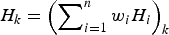 $H_k = \left( {\sum\nolimits_{i = 1}^n {w_i H_i}} \right)_k $ , with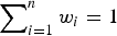 $\sum\nolimits_{i = 1}^n {w_i} = 1$ . We propose calculating the error propagation from the data points to the grid nodes using the same weighted combination, but now applied to the errors instead of the ice thicknesses:

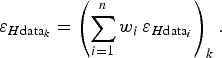(2) $$\varepsilon _{H{\rm data}_k} = \left( {\sum\limits_{i = 1}^n {w_i \,\varepsilon _{H{\rm data}_i}}} \right)_k. $$

This implies an assumption of linear dependence between the error at the grid point and the errors at the neighbouring data points. Due to the unit summation of the weights, the error in the data propagated by Eqn (2) to a grid node is a weighted mean of the errors in the data involved. This is a reasonable approximation, conservative in most cases, as explained below.

Negative ice thicknesses are physically meaningless, so the interpolation scheme must preserve the positive values of the interpolated ice thickness. This can be achieved by using non-negative interpolation weights, such as positive kriging (e.g. Szidarovszky and others, Reference Szidarovszky, Baafi and Kim1987; Deutsch, Reference Deutsch1996; Yamamoto, Reference Yamamoto2000).

Similarly to what we do in Eqn (2), Herzfeld (Reference Herzfeld2004) proposed the use of the interpolation weights for the error propagation from the data points to the grid nodes in the case of kriging interpolation, but she used the root of the squared summation of the n weighted neighbouring values $\varepsilon _{H{\rm data}_k} = \left( {\sum\nolimits_{i = 1}^n {w_i^2 \varepsilon _{H{\rm data}_i} ^2}} \right)_k^{{\rm 1/2}} $ (as if these errors were independent), or, in a simplified version, using the RMS value of the neighbouring errors $\varepsilon _{H{\rm data}_k} = \left( {\sum\nolimits_{i = 1}^n {w_i^2 \left( {{{\sum\nolimits_{i = 1}^n {\varepsilon _{H{\rm data}_i} ^2}} / n}} \right)}} \right)_k^{1/2} $ . However, this expression provides error propagation that does not average the surrounding data errors. If positive kriging is used, and taking into account the unit summation of the ordinary kriging weights, Herzfeld's assumption implies a decrease in the squared values of the weights, so this gives error estimates at the grid nodes much lower than those at surrounding data points, especially when n is large. For instance, let us suppose that a dataset consists of four data points, all with the same value H and the same error E, located at the corners of a square. If we interpolate at the centre of the square, we would expect to get H as the interpolated value and E as its error propagated to the central point. However, assigning a weight of 0.25 to each data point, the interpolated value is indeed H, but the propagated error obtained using the nonlinear method by Herzfeld is 0.5 E $([4(0.25^2 E^2 )]^{1/2} )$ . If, instead, we use Eqn (2), then the error propagated to the central point is E. On the other hand, if not all the weights were positive, larger absolute values of the weights could be involved, still preserving the unit summation. This could imply very large errors at the grid nodes, even several times larger than those at the surrounding data points. For instance, using a similar dataset with four points as before, if the interpolation weights were for example 5, −6, 10, −8, the propagated error using again the non-linear method would be 15 E $((5^2 E^2 + 6^2 E^2 + 10^2 E^2 + 8^2 E^2 )^{1/2} )$ , while, using Eqn (2), the error propagated to the central point is again E.

Because of the above reasons, we are in favour of the linear approach involved in Eqn (2). No matter whether the interpolation weights used are positive or not, Eqn (2) provides, due to the unitary weight summation, an error at each grid point that averages those at the surrounding data points. We thus obtain a reasonable approximation, conservative in the case of using positive weights.

6. ICE-THICKNESS ERROR OF THE DEM

Propagation of the errors in the data to the grid nodes produces resultant errors, $\varepsilon _{H{\rm data}_k} $ , at the grid nodes. In turn, the interpolation errors at the grid nodes, $\varepsilon _{H{\rm int}_k} $ , can be estimated using the DEF. Assuming that in practice these errors can be considered independent, they can be combined as the root of their squared summation, obtaining the total ice-thickness error associated with each grid node,

(3) $$\varepsilon _{H_k} = \sqrt {\varepsilon _{H{\rm data}_k} ^2 + \varepsilon _{H{\rm int}_k} ^2} {\rm.} $$

The propagation of data errors to the grid nodes increases the spatial correlation of the associated errors, smoothing their variability. Consequently, the distribution of errors at the grid nodes will in general be narrower than the error distribution that would be obtained if the data were hypothetically located at the grid points.

Applying Eqn (3) to the grid nodes we obtain an error map of the DEM. However, sometimes it can be useful to characterize the overall quality of the ice-thickness DEM, using a single parameter, for example to estimate the ice-volume error (Martín-Español and others, Reference Martín-Español, Lapazaran, Otero and Navarro2016; this issue (Paper III)), to evaluate the overall quality of DEMs, or to compare their accuracy. In these cases, we can use the RMS value of the errors at the grid nodes,

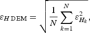(4) $$\varepsilon _{H\,{\rm DEM}} = \sqrt {\displaystyle{1 \over N}\sum\limits_{k = 1}^N {\varepsilon _{H_k} ^2}}, $$

and this parameter will be less sensitive to the above-mentioned smoothing. Note, on the other hand, that the quality of an ice-thickness DEM cannot be calculated directly as the RMS of the errors in the data, because the data distribution, in particular in the case of GPR data, is uneven.

7. CASE STUDY: WERENSKIOLDBREEN

Following the above-discussed techniques, we here present a complete study of the errors for the DEM of ice thickness of Werenskioldbreen, a land-terminating polythermal glacier in Svalbard (Fig. 4).

Fig. 4.

Location of Werenskioldbreen in Svalbard and the dataset used to construct the ice-thickness DEM of Werenskioldbreen. The whole dataset of ice thickness is represented using colour scale and the ice divide with Tuvbreen is shown as a thin black curve in the south-east. The dataset is made of three different types of data: ice-thickness data obtained by means of GPR profiling, zero-ice-thickness boundary points and synthetic data estimated at some non-surveyed tributary glaciers (marked with orange arrows).

The maximum distance between glacier points is ~7 km, while the maximum distance between any grid point and its nearest data point is ~525 m, with a mean value of ~100 m. Thus, the coverage of the glacier surface by the GPR profiles is relatively dense, yet large areas remain devoid of data, as is usual with GPR profiling. This includes both large areas between distant GPR profiles and small non-surveyed tributary glaciers (in fact, small lateral glacier cirques supplying ice to the main glacier trunk). The details of the GPR survey, the data processing and the analysis of the associated errors can be found in Paper I. The ice thickness of the entire boundary is set to zero, except for the ice divide with Tuvbreen (a tributary of Hansbreen), to the south-east. By setting the boundary ice thickness to zero however, interpolation of ice thickness in the non-GPR-surveyed tributaries is biased towards unrealistically low values. To counter this issue, we therefore added to the ice-thickness dataset some additional ice-thickness data points obtained using a slightly modified version of the tributary thickness function for Svalbard glaciers described by Navarro and others (Reference Navarro2014). In our implementation of their method, we obtained regressions both for the normalized amplitudes and the normalized errors. Since, in the case of Werenskioldbreen GPR profiles, there are no measurements of ice thickness at the zones of confluence of the tributaries with the main trunk of the glacier, we increased quadratically the estimated errors by half of the estimated ice thickness. The entire ice-thickness dataset resulting from this addition of data is shown in Figure 4.

We interpolated the ice thickness of the glacier using ordinary kriging to a 50 m × 50 m grid, and found no 2-D geometric anisotropy (e.g. Wackernagel, Reference Wackernagel2003). The resulting ice-thickness DEM is shown in Figure 5a, and has a mean value of 107.65 m, with standard deviation of 73.37 m and maximum gridded value of 276.71 m. We calculated the distance-bias and distance-error functions as explained earlier. The results are shown in Figures 3c, d. The point-dependent interpolation bias applied to each of the grid points yields a DEM of bias, shown in Figure 5b (mean value of 4.41 m, standard deviation of 6.00 m and maximum value of 42.55 m). The final, bias-corrected ice-thickness DEM of Werenskioldbreen, obtained as a point-by-point summation of the interpolated ice thickness and the interpolation bias, is shown in Figure 5c. It has a mean value of 112.31 m, with standard deviation of 74.15 m and maximum gridded value of 277.00 ± 7.24 m (error estimated as described later).

Fig. 5.

DEM of ice thickness of Werenskioldbreen. The colour scale is common for the three panels. (a) DEM of ice thickness obtained by direct interpolation of the data. (b) DEM of interpolation bias obtained applying the DBF to the grid points. Since the bias is negative (Fig. 3c), it is shown with reversed sign, to use a common scale. (c) Final DEM of ice thickness of Werenskioldbreen, obtained as point-by-point summation of the DEMs in (a) and (b).

Let us now analyse the errors in the ice-thickness DEM. The errors in the value of the ice-thickness data, $\varepsilon _{H_i} $ , are shown in Figure 6a. As discussed in Paper I, those corresponding to the GPR data were between 3.32 m (vertical resolution of the 25 MHz radar) and 6.61 m. To the zero-thickness boundary points we assigned a zero error in the value of ice thickness (so all of their error in thickness will correspond to the error due to boundary uncertainty). The errors for the synthetic ice-thickness data points added at some tributaries using our modified version of the tributary thickness function of Navarro and others (Reference Navarro2014), however, were much larger, up to 71.20 m, due to the above-mentioned lack of GPR data at the zones of confluence of the tributaries with the main trunk of the glacier.

Fig. 6.

Ice-thickness errors of the dataset. The colour scale is common for the three panels and for the next Figures. (a) Error in the value of ice thickness, $\varepsilon _{H_i} $ (boundary dots not shown, because of their zero error). (b) Error in ice-thickness due to the uncertainty in horizontal positioning, $\varepsilon _{Hxy_i} $ . (c) Error in ice thickness of the data, $\varepsilon _{H{\rm data}_i} $ , obtained as combination, using Eqn (1), of the errors shown in (a) and (b).

Figure 6b shows the positioning-related ice-thickness error for each data point, $\varepsilon _{Hxy_i} $ . For the GPR measurement points, we estimated $\varepsilon _{Hxy_i} $ as described in Paper I. To obtain the uncertainty in position at each boundary point, we adopted an 8% error in area (i.e. p = 0.08) after Nuth and others (Reference Nuth2013), which for Werenskioldbreen translates as an $\varepsilon _{xy_i} $ of 48 m. The errors in ice thickness due to uncertainty in position of the boundary have a mean value of 6.13 m, with standard deviation of 5.75 m and a maximum value of 39.03 m. Such errors at the boundary are much larger than those of GPR data, because the uncertainty in horizontal positioning and the gradient of ice thickness are both large at the glacier boundaries of Werenskioldbreen. Finally, we assigned to the synthetic ice-thickness values calculated at some tributaries, the same uncertainty in horizontal positioning as that of the boundary points (ε _xy  = 48 m), because the positions of the estimated ice-thickness points in these tributaries were tied to the glacier boundaries. This implied positioning-related ice-thickness errors at the synthetic points in the tributaries reaching 35.32 m (mean value, 10.55 m; standard deviation, 6.02 m).

Figure 6c shows the error in ice thickness of the data, $\varepsilon _{H{\rm data}_i} $ , obtained using Eqn (1), as combination of the errors in value, $\varepsilon _{H_i} $ (Fig. 6a) and those due to uncertainty in position, $\varepsilon _{Hxy_i} $ (Fig. 6b).

We then propagated the errors in the data points to the grid points by means of Eqn (2), using the same weights of the kriging interpolation. Figure 7a shows the resulting DEM of propagated errors (mean value, 7.20 m; standard deviation, 7.24 m; maximum value, 69.02 m). The interpolation errors, characterized by the DEF (Fig. 3d), were then applied to the grid points, producing the DEM of interpolation error shown in Figure 7b (mean value, 9.93 m; standard deviation, 7.82 m; maximum value, 47.42 m). Following Eqn (3), the resulting root of the squared summation of both previous DEMs, calculated point by point, is shown in Figure 7c (mean value, 13.41 m; standard deviation, 9.17 m; maximum value, 69.11 m). It represents the final DEM of ice-thickness errors associated with the ice-thickness DEM of Werenskioldbreen shown in Figure 5c. Finally, we estimated the overall error of the DEM of ice thickness of Werenskioldbreen using Eqn (4), getting ε _H DEM = 16.24 m.

Fig. 7.

(a) DEM of errors propagated from the data points to the grid points using Eqn (2). (b) DEM of interpolation errors at the grid points, obtained applying the DEF to every grid point. (c) Final DEM of error in ice thickness, associated with the DEM of ice thickness shown in Figure 5c.