


1. Introduction
Accreting white dwarf binaries are semi-detached binary systems in which a white dwarf primary is accreting matter from a Roche-lobe-filling secondary star. These system can belong to two different types of object: cataclysmic variables (CVs) and AM Canum Venaticorum (AM CVn) stars.
CVs (e.g. Warner Reference Warner1995) have orbital periods typically between 80 min and 10 h and their donors are hydrogen-rich red dwarfs. There are, however, also examples of CVs with longer orbital periods and sub-giant evolved stars as donors. The transferred matter forms an accretion disc around a white dwarf when no strong magnetic field is present. The accretion disc can undergo transitions between low and high-temperature states, which results in events called dwarf nova outbursts, during which the disc’s brightness increases by several magnitudes. The dwarf nova outbursts typically display bi-modality in their duration which is most evident in the case of SU UMa type of CVs. This type of CVs exhibits normal dwarf nova outbursts and also longer and more energetic superoutbursts. The magnetic CVs can be divided in polars (disc-less systems with accretion through the magnetic field lines) and intermediate polars, where there is a disc formed near the donor star and the matter is later transferred to the WD through magnetic lines. Outbursts in intermediate polars have been observed but are not common (e.g. Hameury & Lasota Reference Hameury and Lasota2017).
The evolutionary models for CVs with donors resembling a main sequence star at the onset of the accretion predict a period minimum $P_{\mathrm{min}}\simeq82\,\mathrm{min}$
which agrees with the observed population of such CVs (Knigge, Baraffe, & Patterson Reference Knigge, Baraffe and Patterson2011), even though the evolutionary models predict more CVs around the period minimum than is observed (Inight et al. Reference Inight2023b; Muñoz-Giraldo, Stelzer, & Schwope Reference Muñoz-Giraldo, Stelzer and Schwope2024). There are also CVs with orbital periods below the period minimum (see for example Breedt et al. Reference Breedt, Gänsicke, Marsh, Steeghs, Drake and Copperwheat2012; Green et al. Reference Green2020; Kára et al. Reference Kára, Zharikov, Wolf, Vaidman, Agishev, Khokhlov and Chavez2025; Green, van Roestel, & Wong Reference Green, van Roestel and Wong2025) which are thought to originate from systems with evolved donors at the onset of the mass accretion. While spectra of these systems show hydrogen lines, they exhibit also strong helium lines.
$P_{\mathrm{min}}\simeq82\,\mathrm{min}$
which agrees with the observed population of such CVs (Knigge, Baraffe, & Patterson Reference Knigge, Baraffe and Patterson2011), even though the evolutionary models predict more CVs around the period minimum than is observed (Inight et al. Reference Inight2023b; Muñoz-Giraldo, Stelzer, & Schwope Reference Muñoz-Giraldo, Stelzer and Schwope2024). There are also CVs with orbital periods below the period minimum (see for example Breedt et al. Reference Breedt, Gänsicke, Marsh, Steeghs, Drake and Copperwheat2012; Green et al. Reference Green2020; Kára et al. Reference Kára, Zharikov, Wolf, Vaidman, Agishev, Khokhlov and Chavez2025; Green, van Roestel, & Wong Reference Green, van Roestel and Wong2025) which are thought to originate from systems with evolved donors at the onset of the mass accretion. While spectra of these systems show hydrogen lines, they exhibit also strong helium lines.
AM CVns (e.g. Ramsay et al. Reference Ramsay2018; Green et al. Reference Green, van Roestel and Wong2025) have orbital periods typically between 5 and 70 min and their donors are hydrogen-poor and helium rich white dwarfs or semi-degenerate stars. Their spectra show helium lines and are devoid of hydrogen lines. The only two systems classified as AM CVns which show optical hydrogen lines are HM Cnc ( $P_{\mathrm{min}}=5.35\,\mathrm{min}$
) and 3XMM J0510-6703 (
$P_{\mathrm{min}}=5.35\,\mathrm{min}$
) and 3XMM J0510-6703 ( $P_{\mathrm{min}}=23.6\,\mathrm{min}$
). These two systems are considered to be direct progenitors of AM CVns in a short-lived phase of accretion of the donor’s thin hydrogen shell (Green et al. Reference Green, van Roestel and Wong2025). HM Cnc is also one of two known AM CVns showing Lyman
$P_{\mathrm{min}}=23.6\,\mathrm{min}$
). These two systems are considered to be direct progenitors of AM CVns in a short-lived phase of accretion of the donor’s thin hydrogen shell (Green et al. Reference Green, van Roestel and Wong2025). HM Cnc is also one of two known AM CVns showing Lyman $\alpha$
absorption line (Munday et al. Reference Munday2023), the other system is CP Eri (Sion et al. Reference Sion, Solheim, Szkody, Gaensicke and Howell2006).
$\alpha$
absorption line (Munday et al. Reference Munday2023), the other system is CP Eri (Sion et al. Reference Sion, Solheim, Szkody, Gaensicke and Howell2006).
Similarly to CVs, AM CVns can host an accretion discs around the white dwarfs which can exhibit outbursts of diverse behaviour caused by transitions between low and high-temperature states (Duffy et al. Reference Duffy2021). Many AM CVns show normal outbursts and superoutburst, similar to CVs of the type SU UMa. Superoutbursts of AM CVns can also be followed by a series of normal outbursts called rebrightenings and a slow decline to the system’s quiescence brightness, which are properties typical also for CVs of the type WZ Sge, a subtype of SU UMa CVs (Kato Reference Kato2015g). Due to the compactness of AM CVn systems which limits the size of their disc, the duration of superoutbursts and normal outbursts tends to be short and they show rapid changes of brightness. These properties have posed a challenge to the ground-based detection of AM CVns. This was demonstrated by Pichardo Marcano et al. (Reference Pichardo Marcano, Rivera Sandoval, Maccarone and Scaringi2021) who also showed how continuous photometry from space-based observatories can be used to study the characteristics of AM CVn outbursts in detail.
The current sample of known AM CVn contains about 100 systems (Green et al. Reference Green, van Roestel and Wong2025) which is only a small fraction when compared to the known CVs (Downes et al. Reference Downes, Webbink, Shara, Ritter, Kolb and Duerbeck2001, Reference Downes, Webbink, Shara, Ritter, Kolb and Duerbeck2006; Ritter & Kolb Reference Ritter and Kolb2003, Reference Ritter and Kolb2011; Jackim et al. Reference Jackim, Szkody, Hazelton and Benson2020). Green et al. (Reference Green, van Roestel and Wong2025) showed that currently known space density of AM CVns predicts about 50 of these systems within $500\,\mathrm{pc}$
while only about 30 systems are known in this region. AM CVns are key laboratories for study of the accretion physics (e.g. Kotko et al. Reference Kotko, Lasota, Dubus and Hameury2012), they are potential progenitors of sub-luminous supernovae.Ia (Bildsten et al. Reference Bildsten, Shen, Weinberg and Nelemans2007), and they are expected to be important sources of low frequency gravitational waves (e.g. Nelemans, Yungelson, & Portegies Zwart Reference Nelemans, Yungelson and Portegies Zwart2004; Scaringi et al. Reference Scaringi, Breivik, Littenberg, Knigge, Groot and Veresvarska2023). Hence, it is important to understand their evolution, characterise their mass transfer and mass accretion and the physical processes which govern their outbursts. For that, it is essential to first identify the largest number of AM CVns and thus, create statistically significant sample which will explore full parameter space of these systems and probe their diverse behaviour. While binary systems can be classified as AM CVn candidates based on photometric observations, spectroscopy is the only way to unambiguously determine whether the donor is a hydrogen-poor and helium-rich star and therefore spectroscopic studies are necessary for identification and/or confirmation of new AM CVns, as was done, for example, by Carter et al. (Reference Carter2014), van Roestel et al. (Reference van Roestel2021), van Roestel et al. (Reference van Roestel2022), Aungwerojwit et al. (Reference Aungwerojwit2025).
$500\,\mathrm{pc}$
while only about 30 systems are known in this region. AM CVns are key laboratories for study of the accretion physics (e.g. Kotko et al. Reference Kotko, Lasota, Dubus and Hameury2012), they are potential progenitors of sub-luminous supernovae.Ia (Bildsten et al. Reference Bildsten, Shen, Weinberg and Nelemans2007), and they are expected to be important sources of low frequency gravitational waves (e.g. Nelemans, Yungelson, & Portegies Zwart Reference Nelemans, Yungelson and Portegies Zwart2004; Scaringi et al. Reference Scaringi, Breivik, Littenberg, Knigge, Groot and Veresvarska2023). Hence, it is important to understand their evolution, characterise their mass transfer and mass accretion and the physical processes which govern their outbursts. For that, it is essential to first identify the largest number of AM CVns and thus, create statistically significant sample which will explore full parameter space of these systems and probe their diverse behaviour. While binary systems can be classified as AM CVn candidates based on photometric observations, spectroscopy is the only way to unambiguously determine whether the donor is a hydrogen-poor and helium-rich star and therefore spectroscopic studies are necessary for identification and/or confirmation of new AM CVns, as was done, for example, by Carter et al. (Reference Carter2014), van Roestel et al. (Reference van Roestel2021), van Roestel et al. (Reference van Roestel2022), Aungwerojwit et al. (Reference Aungwerojwit2025).
Here we present a spectroscopic and photometric study of AM CVn candidates with the aim of confirming these systems and thus increasing the population number. The available photometric observations obtained from various ground-based observatories and from the Transiting Exoplanet Survey Satellite (TESS) mission were used to characterise the outbursts of the targets and to search for periodic variations.
2. Observations
2.1. Target selection
The sample of selected targets consists of transient sources identified with the All-Sky Automated Survey for SupernovaeFootnote a (ASAS-SN; Shappee et al. Reference Shappee2014; Kochanek et al. Reference Kochanek2017), the Zwicky Transient Facility (ZTF) survey,Footnote b the database of American Association of Variable Star ObserversFootnote c (AAVSO; Kloppenborg Reference Kloppenborg2025) and the Variable Stars Network (VS-NET).Footnote d They were classified as AM CVn candidates based on the properties of their light curves such as short duration of outbursts and superoutbursts, rapid luminosity rise and decline, blue colour of the target, and brightness variations with short periodicity. Multiple targets were observed by amateur astronomers who managed to detect superhump variations during the superoutbursts, which allowed to constrain orbital periods of the targets, as superhump periods are typically a few percent longer than orbital periods. These estimates were typically reported as an alert in the VSNET.
Figure 1 shows the finding charts of the selected targets. During the realisation of this work four of the targets (ASASSN-15kf, ASASSN-19ct, ASASSN-20pv, and ASASSN-21hc) were classified as confirmed AM CVn system by Green et al. (Reference Green, van Roestel and Wong2025) based on the presence of outbursts and short orbital period, but no spectroscopic observations were presented prior to our study. We also included two AM CVn systems which have been previously spectroscopically analysed. One of them is ASASSN-17fp, which was observed by Cartier et al. (Reference Cartier2017) during its superoutburst. We included this target with the aim to obtain its spectrum during quiescence. The second target is a well-studied V744 And, also known as Gaia21cxj or SDSSJ0129+3842, (e.g. Ramsay et al. Reference Ramsay, Barclay, Steeghs, Wheatley, Hakala, Kotko and Rosen2012; Kupfer et al. Reference Kupfer, Groot, Levitan, Steeghs, Marsh, Rutten and Nelemans2013) which we included for comparison purposes.
Finding charts for observed targets, the images are blue bands from the Digitized Sky Survey 2 (DSS2, Lasker et al. Reference Lasker, Doggett, McLean, Sturch, Djorgovski, de Carvalho and Reid1996).

TESS light curves of four targets showing various types of outburst behaviour and quiescent states. Different superoutbursts phases of ASASSN-19ct are highlighted by green, orange, and brown colours and correspondingly labelled, measurements with low-quality flags are shown in light blue colour.

2.2. Ground-based photometric data
For all targets we obtained available archival photometry from the ZTF, ASAS-SN, AAVSO and the Asteroid Terrestrial-impact Last Alert System (ATLAS) survey (Tonry et al. Reference Tonry2018). We created light curves to look for signs of outburst activity. We used the Modified Julian Date reference system for all ground based datasets.
For analysis of the targets and their comparison with other stars we also used photometry from the Sloan Digital Sky Survey (SDSS; Alam et al. Reference Alam2015), the Panoramic Survey Telescope and the Rapid Response System (Pan-STARRS; Chambers et al. Reference Chambers2016; Flewelling et al. Reference Flewelling2020), and the SkyMapper Southern Sky Survey (Onken et al. Reference Onken, Wolf, Bessell, Chang, Luvaul, Tonry, White and Da Costa2024a; Onken et al. Reference Onken, Wolf, Bessell, Chang, Luvaul, Tonry, White and Da Costa2024b).
2.3. Gemini observatory spectroscopy
Spectroscopic data were obtained with the 8.1-m telescopes at the international Gemini Observatory located on Maunakea in Hawai’i and Cerro Pachón in Chile. The observations were taken under the programs GN-2023B-Q-310 and GS-2024A-Q-311 in years 2023 and 2024 (PI-Rivera Sandoval), a log of observations is presented in Table 1. All spectra were obtained with GMOS spectrograph (Hook et al. Reference Hook, Jørgensen, Allington-Smith, Davies, Metcalfe, Murowinski and Crampton2004; Gimeno et al. Reference Gimeno2016) equipped with GG455 broad band filter and R400 grating ( $R \sim 1900$
) in case of target ASASSN-18abl and R150 low-resolution grating (
$R \sim 1900$
) in case of target ASASSN-18abl and R150 low-resolution grating ( $R \sim 600$
) for the other systems. Targets were observed in
$R \sim 600$
) for the other systems. Targets were observed in $4\times1$
binning, except for ASASSN-18abl, which was observed in
$4\times1$
binning, except for ASASSN-18abl, which was observed in $2\times1$
binning. Observation of each targets consist of multiple exposures, which allowed us to use spectral dithering to minimise the effects of the gaps between individual CCDs on the final combined spectra whose typical signal-to-noise ratio is
$2\times1$
binning. Observation of each targets consist of multiple exposures, which allowed us to use spectral dithering to minimise the effects of the gaps between individual CCDs on the final combined spectra whose typical signal-to-noise ratio is ${\sim}{20}$
. The spectra cover wavelengths between
${\sim}{20}$
. The spectra cover wavelengths between $4\,800\,\unicode{x00C5}$
and
$4\,800\,\unicode{x00C5}$
and $10\,000\,\unicode{x00C5}$
, apart from ASASSN-15na and ASASSN-18abl, for which the upper bound is about
$10\,000\,\unicode{x00C5}$
, apart from ASASSN-15na and ASASSN-18abl, for which the upper bound is about $9\,100\,{\unicode{x00C5}}$
due to low signal at longer wavelengths in case of the former target and observational configuration in case of the later target.
$9\,100\,{\unicode{x00C5}}$
due to low signal at longer wavelengths in case of the former target and observational configuration in case of the later target.
Log of Gemini observations listing observed targets, their type, J2000 coordinates (RA, DEC), spectrograph used for observation, date of observation, exposure time of individual spectra $t_{\mathrm{exp}}$
, and number of exposures
$t_{\mathrm{exp}}$
, and number of exposures $N_{\mathrm{exp}}$
.
$N_{\mathrm{exp}}$
.

All spectra were reduced using the DRAGONS data reduction software (Labrie et al. Reference Labrie2023; Simpson et al. Reference Simpson, Labrie, Teal, Berke, Turner, Smirnova and Vacca2025). All spectra were flux-calibrated but low flux at the ends of the wavelength ranges rendered the flux-calibration for some of the targets unreliable. The flux-calibrated spectra are presented in Figure B1 in the appendix.
2.4. TESS data
In this work, we use Full-Frame Images (FFIs) and Target Pixel Files (TPFs) of TESS (Ricker et al. Reference Ricker2015) to perform a high-cadence investigation of the outburst activity in our targets. TESS FFIs provide continuous photometric monitoring across multiple observational sectors in various cadence modes (30 min, 10 min, and 200 s) and TPFs provide cutouts of FFIs for selected targets and their light curves with cadences of 2 min and in some cases also 20 s. Both FFIs and TPFs can be used for detailed light curves analysis (Ricker et al. Reference Ricker2015). The observational data were queried and downloaded using the Python package Lightkurve (Lightkurve Collaboration et al. 2018), light curves extracted from FFIs were obtained using aperture photometry method. To ensure high quality of the data, we excluded all measurements with the TESS quality flag $q \gt 0$
to remove instrumental and observational artefacts. Times of observations were converted from Barycentric TESS Julian Date (BTJD) to Modified Julian Date (MJD) using the astropy.time package, the flux measurements are given in electrons per second (e/s) (Astropy Collaboration et al. 2022).
$q \gt 0$
to remove instrumental and observational artefacts. Times of observations were converted from Barycentric TESS Julian Date (BTJD) to Modified Julian Date (MJD) using the astropy.time package, the flux measurements are given in electrons per second (e/s) (Astropy Collaboration et al. 2022).
Table 2 gives the overview of TESS data available for targets from our study.
Summary of the four targets with available TESS photometry with detected superoutbursts (SOs), outbursts (OBs), periods and the uncertainties derived from half-widths at half-maximum (FWHM/2) of corresponding peak in Lomb-Scargle periodogram.
 $^{(a)}$
Superhump period.
$^{(a)}$
Superhump period. $^{(b)}$
Orbital period.
$^{(b)}$
Orbital period.
FWHM for selected He I lines of AM CVn systems.

Separation of the double-peaked profiles for selected He I lines of AM CVn systems.

3. Analysis
3.1. Blackbody fitting
Given the low resolution of our spectra and relatively low signal-to-noise, we fitted the continuum of the flux-calibrated spectra with a blackbody model to characterise its slope instead of a more complicated model. As the flux calibration was problematic in some parts of the spectra, especially near the blue end of the observed range, we excluded these wavelength ranges for the fitting. Before fitting, we corrected the spectra for reddening. We used the three-dimensional map of dust reddening created by Green et al. (Reference Green, Schlafly, Zucker, Speagle and Finkbeiner2019) as the primary source, which allowed us to estimate the reddening correction according to the target’s position on sky as well as its distance. As this map covers only sky north of declination of $-30^\circ$
, four of our targets are not included in its region. Therefore, for ASASSN-20pv and ASASSN-21hc we used reddening provided by the three-dimensional map created by Zucker et al. (Reference Zucker2025) which covers the southern Galactic plane. In cases of ASASN-15na and ASASSN-19ct, which are not located within the region of this map, we used full Galactic reddening from Schlegel, Finkbeiner, & Davis (Reference Schlegel, Finkbeiner and Davis1998).
$-30^\circ$
, four of our targets are not included in its region. Therefore, for ASASSN-20pv and ASASSN-21hc we used reddening provided by the three-dimensional map created by Zucker et al. (Reference Zucker2025) which covers the southern Galactic plane. In cases of ASASN-15na and ASASSN-19ct, which are not located within the region of this map, we used full Galactic reddening from Schlegel, Finkbeiner, & Davis (Reference Schlegel, Finkbeiner and Davis1998).
The temperatures corresponding to the best blackbody fit are listed in Table 5. The optical flux in AM CVn systems consists of contributions from different components, namely the primary star, the donor, the accretion disc, and the bright spot. Therefore, while the temperature derived by fitting the spectrum with a single blackbody spectrum can reflect the temperature of the WD primary to an extent, its value can be affected by radiation from the other components.
Properties of the studied systems.

Parallaxes are taken from the Gaia DR3 catalogue (Gaia Collaboration 2022; Gaia Collaboration et al. 2023), the distance correspond to geometric distances derived by Bailer-Jones et al. (Reference Bailer-Jones, Rybizki, Fouesneau, Demleitner and Andrae2021) from Gaia EDR3 catalogue, superhump periods are marked by (sh). $^{\rm a}$
Period listed in Green et al. (Reference Green, van Roestel and Wong2025).
$^{\rm a}$
Period listed in Green et al. (Reference Green, van Roestel and Wong2025). $^{\rm b}$
Period determined in this work.
$^{\rm b}$
Period determined in this work.
We also tested fitting a blackbody spectrum to the spectral energy distribution (SED) of the targets using the web tool VOSA (Bayo et al. Reference Bayo, Rodrigo, Barrado Y Navascués, Solano, Gutiérrez, Morales-Calderón and Allard2008) with which we obtained similar values of blackbody temperature.
3.2. Widths and peak separations of selected emission lines
The profiles of emission lines originating in the accretion disc are related to the disc velocities and inclination of the system. Usually, they may appear double-peaked, which is a typical profile for a disc viewed at an angle, and their separation can be used to infer the projection of velocity at the outer edge of the disc (Smak Reference Smak1981; Casares Reference Casares2016).
We measured full widths at half maximum (FWHMs) for selected He I emission lines in normalised spectra of our candidates. To determine FWHM of the lines, we fitted each line with a Gaussian profile using a Python package SciPy (Virtanen et al. Reference Virtanen2020), the values of FWHM of the best fits are listed in Table 3.
For those spectra that show double-peaked emission lines we measured separation of the peaks, we used the same set of He I lines as in the case of FWHM measurements. To determine the separation, we fitted each line with a model consisting of two identical Gaussian profiles which were shifted from the central wavelength by a value corresponding to half of the separation. Results of the best fits are given in Table 4.
3.3. Analysis of TESS photometry
For selected sources exhibiting apparent outburst activity, we visually isolated the different phases of the outburst to understand their periodic behaviour. In our periodicity analysis, we used the Lomb-Scargle technique (Lomb Reference Lomb1976; Scargle Reference Scargle1982) implemented by Astropy Python packages. This method allows us to find the periodic signal and generate phase-folded light curves using the best-fit period. To evaluate the significance of the periodic signal, we used the False Alarm Probability (FAP) computed by the astropy module. We calculated the threshold levels of 10%, 0.1%, and 0.001% of FAP using the bootstrap method and included them in our periodograms to distinguish the real signal from noise. We fitted the peaks in periodograms with a Gaussian function to determine their positions, which we used as the best period. We estimated the uncertainties as half-widths at half maximum of the Gaussian functions.
4. Results
Nine of the observed targets exhibit spectral features typical for AM CVns, their normalised spectra are shown in Figure 3. All of these spectra show strong He I emission lines and no detectable hydrogen lines. Four of these targets exhibit single-peaked emission line profiles and five of them show double-peaked profiles. The spectra also exhibit blends of emission associated with other elements, such as Mg II or N I.
Three targets show hydrogen emission lines which classifies them as CVs, their normalised spectra are shown in Figure 4. Three targets show spectra that could be consistent with evolved CVs, their normalised spectra are shown in Figure 4.
As all of the targets were previously reported as transients, their long-term light curves show at least one instance of outburst activity. Table 6 lists superoutburst properties of the studied systems which we derived from the long-term light curves presented in Figure C1.
Normalised spectra of AM CVn stars. Positions of prominent spectral lines are marked by vertical lines, blends of multiple lines are marked by thick lines. The dashed red vertical line shows the potential position of H $\alpha$
line which is absent in all of the presented spectra.
$\alpha$
line which is absent in all of the presented spectra.

Top: normalised spectra of CVs. Positions of prominent spectral lines are marked by vertical lines. All presented spectra show hydrogen emission line from the Balmer series, ZTF18aaaasnn and ZTF21abhrevv show also hydrogen emission lines from the Paschen series. Wavelengths of Paschen lines are marked by vertical red lines. H $\alpha$
line of ASASSN-15na shows a clear double-peaked profile. Bottom: normalised spectra of evolved CV candidates. Positions of prominent spectral lines are marked by vertical lines, position of potential helium lines are marked by dashed blue lines. None of the presented spectra show emission lines typical for accretions discs.
$\alpha$
line of ASASSN-15na shows a clear double-peaked profile. Bottom: normalised spectra of evolved CV candidates. Positions of prominent spectral lines are marked by vertical lines, position of potential helium lines are marked by dashed blue lines. None of the presented spectra show emission lines typical for accretions discs.

Superoutburst properties of studied targets. Presented are recurrence times $T_{\mathrm{SO}}$
, superoutburst durations
$T_{\mathrm{SO}}$
, superoutburst durations $\tau_{\mathrm{dur}}$
, amplitudes
$\tau_{\mathrm{dur}}$
, amplitudes $A_{\mathrm{SO}}$
, peak brightnesses, rise rates
$A_{\mathrm{SO}}$
, peak brightnesses, rise rates $\mu_{r}$
, and decline rates
$\mu_{r}$
, and decline rates $\mu_{d}$
. The column of peak brightness lists also the photometric filter used to determine the peak value.
$\mu_{d}$
. The column of peak brightness lists also the photometric filter used to determine the peak value.

Our analysis of TESS light curves identified outburst activity or periodic signals in four targets, each observed across multiple TESS sectors. Figure 2 presents the light curves of these targets, the identified periods are listed in Table 2. Periodic signals of three targets was identified during superoutbursts and were caused by superhumps. The periodicity of ASASSN-20pv was detected during quiescence and we interpret it as orbital period of this system.
Detailed descriptions of our results for each target is presented in Appendix A of the Appendix.
Seven of our targets lie in the region covered by eROSITA catalogue of X-ray sources (Merloni et al. Reference Merloni2024), five of which have X-ray positions located within 6" of their Gaia coordinates. The two systems without an X-ray detection are ASASSN-15na and ASASSN-17fp, which belong to the faintest systems in our sample. Observed X-ray fluxes for selected eROSITA energy bands are listed in Table 7, which also lists X-ray fluxes of Gaia21cxj listed in the Chandra Source catalogue (Evans et al. Reference Evans2024). All eROSITA observations were obtained during quiescence phases of the systems. Gaia21cxj lacks photometric observations coinciding with the Chandra observations, therefore the activity phase during the observations can’t be determined. However, considering the long recurrence times of its outbursts, they were likely obtained during a quiescence phase as well. Seven of our targets have UV photometry in the GALEX catalogue (2017), which provides photometry in two bands: far-UV (FUV, $\lambda_{\mathrm{eff}} \sim 1\,528\,\unicode{x00C5}$
, 1 344–1 786 Å) and near-UV (NUV,
$\lambda_{\mathrm{eff}} \sim 1\,528\,\unicode{x00C5}$
, 1 344–1 786 Å) and near-UV (NUV, $\lambda_{\mathrm{eff}} \sim 2\,310\,\unicode{x00C5}$
, 1 771–2 831 Å). The fluxes derived from the photometry given in the catalogue are listed in Table 8.
$\lambda_{\mathrm{eff}} \sim 2\,310\,\unicode{x00C5}$
, 1 771–2 831 Å). The fluxes derived from the photometry given in the catalogue are listed in Table 8.
X-ray fluxes f of studied AM CVns and their and luminosities L mass accretion rates $\dot{M}$
derived for the combination of listed energy bands. Periods listed for ASASSN-20pv and Gaia21cxj are orbital periods, superhump periods are listed for the other systems. Critical mass accretion rates
$\dot{M}$
derived for the combination of listed energy bands. Periods listed for ASASSN-20pv and Gaia21cxj are orbital periods, superhump periods are listed for the other systems. Critical mass accretion rates $\dot{M}_{\mathrm{crit}}^-$
and
$\dot{M}_{\mathrm{crit}}^-$
and $\dot{M}_{\mathrm{crit}}^+$
were determined using Equation (A.2) of Kotko et al. (Reference Kotko, Lasota, Dubus and Hameury2012).
$\dot{M}_{\mathrm{crit}}^+$
were determined using Equation (A.2) of Kotko et al. (Reference Kotko, Lasota, Dubus and Hameury2012).

UV fluxes of studied system obtained from the GALEX catalogue (Bianchi et al. Reference Bianchi, Shiao and Thilker2017). Period listed in this table represent superhump periods of the systems.

5. Discussion
5.1. Colour-magnitude diagram
Figure 5, left panel, shows the positions of the observed target in a colour-magnitude diagram constructed using absolute Gaia magnitudes $M_G$
and colours based on Gaia’s blue prism (BP) and red prism (RP) magnitudes. Targets ASASSN-15na, ASASSN-17fp, and ASASSN-20la are not included due to a lack of Gaia observations. The diagram also shows the positions of AM CVn stars listed in the catalogue by Green et al. (Reference Green, van Roestel and Wong2025) and CVs from the catalogue by Ritter & Kolb (Reference Ritter and Kolb2003, Reference Ritter and Kolb2011).
$M_G$
and colours based on Gaia’s blue prism (BP) and red prism (RP) magnitudes. Targets ASASSN-15na, ASASSN-17fp, and ASASSN-20la are not included due to a lack of Gaia observations. The diagram also shows the positions of AM CVn stars listed in the catalogue by Green et al. (Reference Green, van Roestel and Wong2025) and CVs from the catalogue by Ritter & Kolb (Reference Ritter and Kolb2003, Reference Ritter and Kolb2011).
Left: Colour-magnitude diagram showing Gaia sources within 200 pc (grey), AM CVns (blue), CVs (orange), AM CVns, and CVs from the studied sample (green stars and red stars, respectively), and targets from the studied sample of other type (purple star). No reddening correction was applied for the presented data. Right: Colour-colour diagram showing stars from the SDSS DR12 catalogue (grey), AM CVns and CVs based on SDSS photometry, and targets from the studied sample based on ZTF, SkyMapper, and PanStarrs1 photometry. Targets with only one available colour index are represented by a line. The dashed line represents the selection criteria used by Carter et al. (Reference Carter2014) for the identification of AM CVns.

All AM CVn stars and CVs analysed in this paper are blue, grouped in a region close to the WD branch, where both of these types can be expected (Abril et al. Reference Abril, Schmidtobreick, Ederoclite and López-Sanjuan2020; Inight et al. Reference Inight2023a ; Green et al. Reference Green, van Roestel and Wong2025), indicating an important contribution from the accreting WD and the inner part of the accretion disc. All of them can be found slightly above the WD sequence, apart from one system, ASASSN-18rg, which is located below that sequence. However, parallax of this system was determined with a large error (see Table 5), which might have affected its vertical position in the diagram.
The diagram shows that AM CVn stars tend to have bluer colours than CVs, even though there is a partial overlap, in which the targets analysed in this work are located. CVs found in this overlap are dominantly short-period CVs with orbital periods bellow 2 h. All AM CVns studied in this paper occupy the region for which
 \begin{equation} \mathrm{BP} - \mathrm{RP} \lt 0.5,\end{equation}
which is true also for approximately 88% of known AM CVns with available Gaia photometry and for approximately 34% of CVs from the catalogue by Ritter & Kolb (Reference Ritter and Kolb2011). Combining the properties of AM CVns from our study and from literature, we can determine the boundaries of region in colour-magnitude diagram occupied by AM CVns as
 \begin{equation}\begin{aligned} -0.3 \lt\mathrm{BP} &- \mathrm{RP} \lt 0.5, \\ 5.5\lt \;&M_G\lt13,\end{aligned}\end{equation}
which is occupied by 89% of known AM CVns, boundaries of this region are marked by black dashed line in Figure 5.
Two clear outliers from the analysed sample are the two stars labelled as ‘other’: ASASSN-18abl and TCP J00505644+5351524. The colour index of these stars shows that they are red objects, and they are located on the main sequence, unlike most of the AM CVn stars and CVs. Given that these systems have shown superoutbursts, their binary nature is confirmed and the lack of emission lines indicate that the red component is clearly dominating the spectrum.
5.2. Colour-colour diagram
Figure 5, right panel, shows a de-reddened colour-colour diagram based on photometry in bands g, r, and i. The photometry for the targets from this work was obtained primarily from ZTF. In cases where ZTF data were not available, we used photometry from SkyMapper and Pan-STARS. Only observation obtained at quiescence were considered. The photometry for known AM CVns and CVs was obtained from SDSS. We adopted reddening values from Schlegel et al. (Reference Schlegel, Finkbeiner and Davis1998) and converted them to corresponding filters by relations derived by Schlafly & Finkbeiner (Reference Schlafly and Finkbeiner2011). We chose to use reddening derived by Schlegel et al. (Reference Schlegel, Finkbeiner and Davis1998) as it was also used in previous studies of AM CVns (for example Roelofs et al. Reference Roelofs2009; Carter et al. Reference Carter2013, Reference Carter2014), which allows us to easily compare our results with those of other authors.
AM CVns from this paper show narrow spread in $g-r$
and they occupy the region for which
$g-r$
and they occupy the region for which
 \begin{equation} g-r \lt -0.11,\end{equation}
which applies also to 84% of known AM CVns and 29% of CVs from the catalogue of Ritter & Kolb (Reference Ritter and Kolb2011). This shows that $g-r$
colour index is a useful parameter for selection of AM CVn candidates. The spread in
$g-r$
colour index is a useful parameter for selection of AM CVn candidates. The spread in $r-i$
is larger and the studied AM CVns have values for which
$r-i$
is larger and the studied AM CVns have values for which
 \begin{equation} r-i \lt 0.06,\end{equation}
which is true also for 88% of known AM CVns and 60% CVs used in this study for comparison.
A similar colour-colour diagram was also presented by Carter et al. (Reference Carter2013), their selection criteria for the identification of AM CVns are marked in the colour-colour diagram by a black dashed line. Five of the AM CVns from this study lie inside of the region fulfilling these criteria, while three lie outside. Two of the outliers, ASASSN-20pv ( $r-i=-0.35$
,
$r-i=-0.35$
, $g-r=-0.50$
) and ASASSN-21hc (
$g-r=-0.50$
) and ASASSN-21hc ( $r-i=0.06$
,
$r-i=0.06$
, $g-r=-0.43$
), lie close to the boundary, while the third one, ASASSN-20lr (
$g-r=-0.43$
), lie close to the boundary, while the third one, ASASSN-20lr ( $r-i=-0.70$
,
$r-i=-0.70$
, $g-r=-1.44$
), is a clear outlier. However, the reddening given by Schlegel et al. (Reference Schlegel, Finkbeiner and Davis1998) for the position of ASASSN-20lr is
$g-r=-1.44$
), is a clear outlier. However, the reddening given by Schlegel et al. (Reference Schlegel, Finkbeiner and Davis1998) for the position of ASASSN-20lr is $E(B-V)=1.47$
which strongly affects the position of the star in the colour-colour diagram and given the fact that Schlegel et al. (Reference Schlegel, Finkbeiner and Davis1998) provides full Galactic reddening, it is likely that the reddening of ASASSN-20lr is overestimated. The three-dimensional extinction map by Green et al. (Reference Green, Schlafly, Zucker, Speagle and Finkbeiner2019) gives for the position of ASASSN-20lr and its Gaia distance
$E(B-V)=1.47$
which strongly affects the position of the star in the colour-colour diagram and given the fact that Schlegel et al. (Reference Schlegel, Finkbeiner and Davis1998) provides full Galactic reddening, it is likely that the reddening of ASASSN-20lr is overestimated. The three-dimensional extinction map by Green et al. (Reference Green, Schlafly, Zucker, Speagle and Finkbeiner2019) gives for the position of ASASSN-20lr and its Gaia distance $E(g-r)=0.35$
. This value is considerably lower than the one of full Galactic reddening and leads to colours
$E(g-r)=0.35$
. This value is considerably lower than the one of full Galactic reddening and leads to colours $r-i=-0.09$
,
$r-i=-0.09$
, $g-r=-0.35$
, which lie within the region occupied by AM CVns.
$g-r=-0.35$
, which lie within the region occupied by AM CVns.
5.3. X-ray and UV luminosities and accretion rates
We computed the X-ray luminosities for our targets with available X-ray data using the Gaia distances determined by Bailer-Jones et al. (Reference Bailer-Jones, Rybizki, Fouesneau, Demleitner and Andrae2021), the resulting values are given in Table 7. All eROSITA observations were obtained during quiescence, which is also likely the case of Gaia21cxj. The luminosities lie in the range between $2.98\times 10^{30}\mathrm{erg}\,\mathrm{s}^{-1}$
and
$2.98\times 10^{30}\mathrm{erg}\,\mathrm{s}^{-1}$
and $29.14\times 10^{30} \, \mathrm{erg}\,\mathrm{s}^{-1}$
, which agrees with the X-ray luminosities of AM CVn studied by Begari & Maccarone (Reference Begari and Maccarone2023), who reported that short-period AM CVns show X-ray luminosities smaller than those predicted by models (van Haaften et al. Reference van Haaften, Nelemans, Voss, Wood and Kuijpers2012) likely due to the boundary layer of short-period systems being optically thick. We computed GALEX-UV luminosities for our targets using an analogous approach, the obtained luminosities are listed in Table 8.
$29.14\times 10^{30} \, \mathrm{erg}\,\mathrm{s}^{-1}$
, which agrees with the X-ray luminosities of AM CVn studied by Begari & Maccarone (Reference Begari and Maccarone2023), who reported that short-period AM CVns show X-ray luminosities smaller than those predicted by models (van Haaften et al. Reference van Haaften, Nelemans, Voss, Wood and Kuijpers2012) likely due to the boundary layer of short-period systems being optically thick. We computed GALEX-UV luminosities for our targets using an analogous approach, the obtained luminosities are listed in Table 8.
The maximal possible luminosity of boundary layer $L_{\mathrm{BL}}$
is according to Frank, King, & Raine (Reference Frank, King and Raine2002, equation 6.6)
$L_{\mathrm{BL}}$
is according to Frank, King, & Raine (Reference Frank, King and Raine2002, equation 6.6)
 \begin{equation} L_{\mathrm{BL}} = \frac{G\,M_1\,\dot{M}}{2\,R_1}\left[ 1-\frac{\Omega_1}{\Omega_{\mathrm{K}}} \right]^2,\end{equation}
where $R_1$
,
$R_1$
, $M_1$
, and
$M_1$
, and $\Omega_1$
are the radius, mass, and surface angular velocity of the primary star, G is the gravitational constant,
$\Omega_1$
are the radius, mass, and surface angular velocity of the primary star, G is the gravitational constant, $\dot{M}$
is the mass accretion rate, and
$\dot{M}$
is the mass accretion rate, and $\Omega_{\mathrm{K}}$
is the Keplerian angular velocity of the boundary layer. If we assume
$\Omega_{\mathrm{K}}$
is the Keplerian angular velocity of the boundary layer. If we assume $\Omega_1 \ll \Omega_{\mathrm{K}}$
and that
$\Omega_1 \ll \Omega_{\mathrm{K}}$
and that $L_{\mathrm{BL}}$
is equal to the X-ray luminosity
$L_{\mathrm{BL}}$
is equal to the X-ray luminosity $L_{\mathrm{X}}$
, we can estimate the mass accretion rate as
$L_{\mathrm{X}}$
, we can estimate the mass accretion rate as
 \begin{equation} \dot{M}=\frac{2\,R_1\,L_{\mathrm{X}}}{G\,M_1}.\end{equation}
However, this equation provides only lower limit on the mass accretion rate, as the assumptions $\Omega_1 \ll \Omega_{\mathrm{K}}$
and
$\Omega_1 \ll \Omega_{\mathrm{K}}$
and $L_{\mathrm{BL}} = L_{\mathrm{X}}$
lead to underestimating the value of
$L_{\mathrm{BL}} = L_{\mathrm{X}}$
lead to underestimating the value of $\dot{M}$
. For the calculations, we assumed
$\dot{M}$
. For the calculations, we assumed $M_1=0.85\,\mathrm{M}_\odot$
and we calculated corresponding radius
$M_1=0.85\,\mathrm{M}_\odot$
and we calculated corresponding radius $R_1 = 0.009\,\mathrm{R}_\odot$
using the relation given by Verbunt & Rappaport (Reference Verbunt and Rappaport1988). The resulting mass accretion rates derived from X-ray and UV luminosities are listed in Tables 7 and 8, respectively. Their values are of orders
$R_1 = 0.009\,\mathrm{R}_\odot$
using the relation given by Verbunt & Rappaport (Reference Verbunt and Rappaport1988). The resulting mass accretion rates derived from X-ray and UV luminosities are listed in Tables 7 and 8, respectively. Their values are of orders $10^{-13}$
–
$10^{-13}$
– $10^{-12}\,\dfrac{\mathrm{M}_\odot}{\mathrm{yr}}$
.
$10^{-12}\,\dfrac{\mathrm{M}_\odot}{\mathrm{yr}}$
.
For the accretion disc to be in an unstable state, in which outburst can occur, its accretion rate needs to be between critical values $\dot{M}_{\mathrm{crit}}^{-}$
and
$\dot{M}_{\mathrm{crit}}^{-}$
and $\dot{M}_{\mathrm{crit}}^{+}$
. Using the same parameters for
$\dot{M}_{\mathrm{crit}}^{+}$
. Using the same parameters for $M_1$
and
$M_1$
and $R_1$
and assuming the disc’s inner radius is the size of accretor and the disc viscosity
$R_1$
and assuming the disc’s inner radius is the size of accretor and the disc viscosity $\alpha_{\mathrm{cold}}=0.1$
we can estimate the critical mass accretion rate
$\alpha_{\mathrm{cold}}=0.1$
we can estimate the critical mass accretion rate $\dot{M}_{\mathrm{crit}}^{-}=1.7\times 10^{-13}\,\mathrm{M}_\odot\,\mathrm{yr}^{-1}$
from the Equation (A.2) of Kotko et al. (Reference Kotko, Lasota, Dubus and Hameury2012) for an AM CVn with 2% of metals. All of the mass accretion rates obtained from the X-ray observations lie above this limit. By assuming a mass ratio
$\dot{M}_{\mathrm{crit}}^{-}=1.7\times 10^{-13}\,\mathrm{M}_\odot\,\mathrm{yr}^{-1}$
from the Equation (A.2) of Kotko et al. (Reference Kotko, Lasota, Dubus and Hameury2012) for an AM CVn with 2% of metals. All of the mass accretion rates obtained from the X-ray observations lie above this limit. By assuming a mass ratio $q=0.03$
(as determined from studies of eclipsing systems, van Roestel et al. Reference van Roestel2022) and
$q=0.03$
(as determined from studies of eclipsing systems, van Roestel et al. Reference van Roestel2022) and $\alpha_{\mathrm{hot}}=0.2$
we can estimate
$\alpha_{\mathrm{hot}}=0.2$
we can estimate $\dot{M}_{\mathrm{crit}}^{+}$
for each target, the estimated values are listed in Table 7.
$\dot{M}_{\mathrm{crit}}^{+}$
for each target, the estimated values are listed in Table 7.
All estimated $\dot{M}_{\mathrm{crit}}^{+}$
are about four orders of magnitude larger than the mass accretion rates obtained from the X-ray observations. This places the studied AM CVns in the unstable disc region, consistent with their observed transient behaviour. Yet, the derived accretion rates are below the values predicted by evolutionary models (Wong & Bildsten Reference Wong and Bildsten2021) for mass transfer rates of the accretion discs. Since our mass accretion rates were determined using only X-ray luminosities, the obtained values can be underestimated if most of the emission comes in the UV, which can be expected from previous studies of AM CVns (e.g. Ramsay et al. Reference Ramsay, Groot, Marsh, Nelemans, Steeghs and Hakala2006). Therefore, the derived values can serve only as a lower limit for the mass accretion rates. This applies especially to short-period systems, for which the accretion rates derived from observed X-ray luminosities are underestimated due to the presence of a likely optically thick boundary layer (Begari & Maccarone Reference Begari and Maccarone2023).
$\dot{M}_{\mathrm{crit}}^{+}$
are about four orders of magnitude larger than the mass accretion rates obtained from the X-ray observations. This places the studied AM CVns in the unstable disc region, consistent with their observed transient behaviour. Yet, the derived accretion rates are below the values predicted by evolutionary models (Wong & Bildsten Reference Wong and Bildsten2021) for mass transfer rates of the accretion discs. Since our mass accretion rates were determined using only X-ray luminosities, the obtained values can be underestimated if most of the emission comes in the UV, which can be expected from previous studies of AM CVns (e.g. Ramsay et al. Reference Ramsay, Groot, Marsh, Nelemans, Steeghs and Hakala2006). Therefore, the derived values can serve only as a lower limit for the mass accretion rates. This applies especially to short-period systems, for which the accretion rates derived from observed X-ray luminosities are underestimated due to the presence of a likely optically thick boundary layer (Begari & Maccarone Reference Begari and Maccarone2023).
Limitations of using only X-ray observations for accretion rate estimation can be seen on the case of ASASSN-19ct for which we determined $\dot{M}_{\mathrm{FUV+NUV}}=61.43\,\times 10^{-13}\,\mathrm{M}_\odot\,\mathrm{yr}^{-1}$
which is about ten times larger value than the one obtained from X-rays. However, due to lack of photometric monitoring coinciding with the GALEX observations, we cannot determine if the UV observations were obtained in quiescence or during a superoutburst. As the recurrence times of superoutbursts of ASASSN-19ct are shorter than one year, it is possible that the large UV flux was caused by a superoutburst.
$\dot{M}_{\mathrm{FUV+NUV}}=61.43\,\times 10^{-13}\,\mathrm{M}_\odot\,\mathrm{yr}^{-1}$
which is about ten times larger value than the one obtained from X-rays. However, due to lack of photometric monitoring coinciding with the GALEX observations, we cannot determine if the UV observations were obtained in quiescence or during a superoutburst. As the recurrence times of superoutbursts of ASASSN-19ct are shorter than one year, it is possible that the large UV flux was caused by a superoutburst.
The mass accretion rate of ASASSN-20gx lies above the limit $\dot{M}_{\mathrm{crit}}^{-}=2.6\,\times 10^{-13}\,\mathrm{M}_\odot\,\mathrm{yr}^{-1}$
, but ASASSN-18rg shows accretion rate
$\dot{M}_{\mathrm{crit}}^{-}=2.6\,\times 10^{-13}\,\mathrm{M}_\odot\,\mathrm{yr}^{-1}$
, but ASASSN-18rg shows accretion rate $\dot{M}_{\mathrm{FUV+NUV}}=2.49_{-1.62}^{+5.24}\,\times 10^{-13}\,\mathrm{M}_\odot\,\mathrm{yr}^{-1}$
which lies just beneath
$\dot{M}_{\mathrm{FUV+NUV}}=2.49_{-1.62}^{+5.24}\,\times 10^{-13}\,\mathrm{M}_\odot\,\mathrm{yr}^{-1}$
which lies just beneath $\dot{M}_{\mathrm{crit}}^{-}$
, however, the critical value is within the estimated uncertainty. The mass accretion rates
$\dot{M}_{\mathrm{crit}}^{-}$
, however, the critical value is within the estimated uncertainty. The mass accretion rates $\dot{M}_{\mathrm{FUV+NUV}}$
of ZTF18aaaasnn, ZTF21abhrevv, and ASASSN-18abl are above the predicted critical accretion rate for CVs
$\dot{M}_{\mathrm{FUV+NUV}}$
of ZTF18aaaasnn, ZTF21abhrevv, and ASASSN-18abl are above the predicted critical accretion rate for CVs $\dot{M}_{\mathrm{crit}}^{-} \approx 0.8 \times 10^{-13}\,\mathrm{M}_\odot\,\mathrm{yr}^{-1}$
(Knigge et al. Reference Knigge, Baraffe and Patterson2011).
$\dot{M}_{\mathrm{crit}}^{-} \approx 0.8 \times 10^{-13}\,\mathrm{M}_\odot\,\mathrm{yr}^{-1}$
(Knigge et al. Reference Knigge, Baraffe and Patterson2011).
We note that mass transfer rates of a sample of AM CVns derived by Ramsay et al. (Reference Ramsay2018) from SEDs are of several orders higher and in agreement with evolutionary models. A difference between $\dot{M}$
derived from SED modelling and from X-rays can be expected, as SED modelling provides
$\dot{M}$
derived from SED modelling and from X-rays can be expected, as SED modelling provides $\dot{M}$
which is characteristic for the mass transfer in the whole accretion disc, while X-rays and UV fluxes provide estimate of accretion onto the white dwarf. The systems analysed by Ramsay et al. (Reference Ramsay2018) also show smaller X-ray luminosities than is predicted by models, as was shown by Begari & Maccarone (Reference Begari and Maccarone2023), which are of the same order as the X-ray luminosities derived in our study.
$\dot{M}$
which is characteristic for the mass transfer in the whole accretion disc, while X-rays and UV fluxes provide estimate of accretion onto the white dwarf. The systems analysed by Ramsay et al. (Reference Ramsay2018) also show smaller X-ray luminosities than is predicted by models, as was shown by Begari & Maccarone (Reference Begari and Maccarone2023), which are of the same order as the X-ray luminosities derived in our study.
5.4. Amplitudes of superoutbursts of AM CVn and CV stars
Figure 7 shows the relation between orbital periods and amplitudes of superoutbursts for AM CVns from this study and from the literature presented by Cannizzo & Ramsay (Reference Cannizzo and Ramsay2019). The amplitudes of superoutbursts were determined from ground-based observations presented in Figure C1, the values are listed in Table 6. The Figure also shows the linear relation derived by Levitan et al. (Reference Levitan, Groot, Prince, Kulkarni, Laher, Ofek, Sesar and Surace2015) for AM CVns with orbital periods between 22 and 37 min. While there is a correlation between the amplitude of superoutbursts and the orbital period (Pearson correlation coefficient $c_{P}=0.6$
), there is a large dispersion especially for longer orbital periods. All but one of the AM CVns from our study shown in the figure have amplitudes larger that it is predicted by the relation derived by Levitan et al. (Reference Levitan, Groot, Prince, Kulkarni, Laher, Ofek, Sesar and Surace2015) (orange dotted line) or the relation which can be derived from the sample presented by Cannizzo & Ramsay (Reference Cannizzo and Ramsay2019) (blue dashed line). The linear relation derived from all AM CVns in this study is
$c_{P}=0.6$
), there is a large dispersion especially for longer orbital periods. All but one of the AM CVns from our study shown in the figure have amplitudes larger that it is predicted by the relation derived by Levitan et al. (Reference Levitan, Groot, Prince, Kulkarni, Laher, Ofek, Sesar and Surace2015) (orange dotted line) or the relation which can be derived from the sample presented by Cannizzo & Ramsay (Reference Cannizzo and Ramsay2019) (blue dashed line). The linear relation derived from all AM CVns in this study is
 \begin{equation} A_{\mathrm{SO}}=(0.11\pm0.03)P_{\mathrm{orb}} + (0.72\pm1.04),\end{equation}
where $A_{\mathrm{SO}}$
is the amplitude and
$A_{\mathrm{SO}}$
is the amplitude and $P_{\mathrm{orb}}$
is the orbital period in minutes. It is possible that some of the previously published amplitudes could be underestimated due to incomplete coverage of the superoutbursts.
$P_{\mathrm{orb}}$
is the orbital period in minutes. It is possible that some of the previously published amplitudes could be underestimated due to incomplete coverage of the superoutbursts.
Top: Distribution of temperatures of the studied targets derived by fitting the continuum of spectra with a black-body model. Typical size of error is of the size of the symbols. Bottom: Relation between orbital periods of AM CVns from this study and their temperatures determined from the black-body model. Typical size of error is of the size of the symbols.

The amplitudes of the confirmed CVs identified in this study are consistent with the amplitude limits established for their orbital period (Coppejans et al. Reference Coppejans, Körding, Knigge, Pretorius, Woudt, Groot, Van Eck and Drake2016; Otulakowska-Hypka, Olech, & Patterson Reference Otulakowska-Hypka, Olech and Patterson2016).
5.5. Superoutburst duration for the AM CVns
By construction, our sample is formed of systems identified through their outbursts. Figure 7 shows the relations between orbital periods and durations of the superoutbursts $\tau_{\mathrm{dur}}$
for the AM CVns from this work and from previous studies (Cannizzo & Ramsay Reference Cannizzo and Ramsay2019; Rivera Sandoval et al. Reference Rivera Sandoval, Maccarone and Pichardo Marcano2020, Reference Rivera Sandoval, Maccarone, Cavecchi, Britt and Zurek2021, Reference Rivera Sandoval, Heinke, Hameury, Cavecchi, Vanmunster, Tordai and Romanov2022). All the AM CVns from our study exhibited superoutbursts with durations between 6 and 10 d and they do not show any strong dependency on the orbital period. Similar short durations were already identified for systems with periods shorter than 35 min (Pichardo Marcano et al. Reference Pichardo Marcano, Rivera Sandoval, Maccarone and Scaringi2021). Interestingly, ASASSN-17fp (51 min) also showed a short duration superoutburst consistent with a disc instability origin, which contrasts with those systems with orbital periods longer than 50 min for which high state activity has been observed to last for years (Rivera Sandoval et al. Reference Rivera Sandoval, Maccarone and Pichardo Marcano2020, Reference Rivera Sandoval, Maccarone, Cavecchi, Britt and Zurek2021) and the origin of which is attributed to EMT. This supports the existence of a dichotomy as observed in ASASSN-21au (Rivera Sandoval et al. Reference Rivera Sandoval, Heinke, Hameury, Cavecchi, Vanmunster, Tordai and Romanov2022). The dichotomy is likely linked to different mass-transfer rates and even disc truncation (Rivera Sandoval et al. Reference Rivera Sandoval, Heinke, Hameury, Cavecchi, Vanmunster, Tordai and Romanov2022).
$\tau_{\mathrm{dur}}$
for the AM CVns from this work and from previous studies (Cannizzo & Ramsay Reference Cannizzo and Ramsay2019; Rivera Sandoval et al. Reference Rivera Sandoval, Maccarone and Pichardo Marcano2020, Reference Rivera Sandoval, Maccarone, Cavecchi, Britt and Zurek2021, Reference Rivera Sandoval, Heinke, Hameury, Cavecchi, Vanmunster, Tordai and Romanov2022). All the AM CVns from our study exhibited superoutbursts with durations between 6 and 10 d and they do not show any strong dependency on the orbital period. Similar short durations were already identified for systems with periods shorter than 35 min (Pichardo Marcano et al. Reference Pichardo Marcano, Rivera Sandoval, Maccarone and Scaringi2021). Interestingly, ASASSN-17fp (51 min) also showed a short duration superoutburst consistent with a disc instability origin, which contrasts with those systems with orbital periods longer than 50 min for which high state activity has been observed to last for years (Rivera Sandoval et al. Reference Rivera Sandoval, Maccarone and Pichardo Marcano2020, Reference Rivera Sandoval, Maccarone, Cavecchi, Britt and Zurek2021) and the origin of which is attributed to EMT. This supports the existence of a dichotomy as observed in ASASSN-21au (Rivera Sandoval et al. Reference Rivera Sandoval, Heinke, Hameury, Cavecchi, Vanmunster, Tordai and Romanov2022). The dichotomy is likely linked to different mass-transfer rates and even disc truncation (Rivera Sandoval et al. Reference Rivera Sandoval, Heinke, Hameury, Cavecchi, Vanmunster, Tordai and Romanov2022).
It is possible that some of previously published durations of superoutbursts might be overestimated due to poor sampling of the light curves, which could cause echo outbursts and fading tails to appear as a part of the superoutburst. The flat superoutburst duration distribution observed in Figure 7 is in agreement with the expected dependency derived for a traditional disc instability model by Cannizzo & Nelemans (Reference Cannizzo and Nelemans2015), who predicts only a relatively modest dependency of $\tau_{\mathrm{dur}} \propto P_{\mathrm{orb}}^{\,0.4}$
. However, as discussed for the case of ASASSN-19ct, it is possible that EMT is also present.
$\tau_{\mathrm{dur}} \propto P_{\mathrm{orb}}^{\,0.4}$
. However, as discussed for the case of ASASSN-19ct, it is possible that EMT is also present.
5.6. Comparison of superoutburst properties of AM CVns and CVs
We determined the rise and decline rates of targets from this study from the corresponding phases of superoutbursts, following similar method as Otulakowska-Hypka et al. (Reference Otulakowska-Hypka, Olech and Patterson2016). Figure 8, left panel, shows relation between orbital periods and superoutburst rise rates $\mu_{r}$
for AM CVns from this study and for CVs analysed by Otulakowska-Hypka et al. (Reference Otulakowska-Hypka, Olech and Patterson2016), the right panel shows analogous relation for decline rates
$\mu_{r}$
for AM CVns from this study and for CVs analysed by Otulakowska-Hypka et al. (Reference Otulakowska-Hypka, Olech and Patterson2016), the right panel shows analogous relation for decline rates $\mu_{d}$
. The central panel then shows the relation between superoutburst amplitudes and durations.
$\mu_{d}$
. The central panel then shows the relation between superoutburst amplitudes and durations.
Otulakowska-Hypka et al. (Reference Otulakowska-Hypka, Olech and Patterson2016) reported that CVs above the period gap ( $P_{\mathrm{orb}} \gt 3\,\mathrm{h}$
) show dependency of rise rates and decline rates of long outbursts and superoutbursts on their orbital periods. The CVs bellow the period gap (
$P_{\mathrm{orb}} \gt 3\,\mathrm{h}$
) show dependency of rise rates and decline rates of long outbursts and superoutbursts on their orbital periods. The CVs bellow the period gap ( $P_{\mathrm{orb}} \lt 2\,\mathrm{h}$
) show large dispersion in both rates with no dependency on orbital period.
$P_{\mathrm{orb}} \lt 2\,\mathrm{h}$
) show large dispersion in both rates with no dependency on orbital period.
All AM CVns show fast changes of brightness during the decline and rise phases of their outbursts. The values of the rise rates are in the range $2.2\,\mathrm{mag}\,\mathrm{d}^{-1} \lesssim \mu_{r}\lesssim5.6\,\mathrm{mag}\,\mathrm{d}^{-1}$
and the values of decline rates lie in the range
$2.2\,\mathrm{mag}\,\mathrm{d}^{-1} \lesssim \mu_{r}\lesssim5.6\,\mathrm{mag}\,\mathrm{d}^{-1}$
and the values of decline rates lie in the range $1.2\,\mathrm{mag}\,\mathrm{d}^{-1} \lesssim \mu_{d} \lesssim2.5\,\mathrm{mag}\,\mathrm{d}^{-1}$
. We note that the CV classified by Otulakowska-Hypka et al. (Reference Otulakowska-Hypka, Olech and Patterson2016) as ER UMa, which lies in the same regions as AM CVns, is a known AM CVn star, CR Boötis. All AM CVns show faster changes of brightness during the rise than during the decline, similarly as majority of CVs analysed by Otulakowska-Hypka et al. (Reference Otulakowska-Hypka, Olech and Patterson2016). However, they show much smaller dispersion in the both rates than the CVs bellow the period gap. WZ Sge stars also exhibit low dispersion of their rise rates, which is even smaller than for AM CVns, their decline rate dispersion is, however, larger and comparable with other type of CVs bellow the period gap.
$1.2\,\mathrm{mag}\,\mathrm{d}^{-1} \lesssim \mu_{d} \lesssim2.5\,\mathrm{mag}\,\mathrm{d}^{-1}$
. We note that the CV classified by Otulakowska-Hypka et al. (Reference Otulakowska-Hypka, Olech and Patterson2016) as ER UMa, which lies in the same regions as AM CVns, is a known AM CVn star, CR Boötis. All AM CVns show faster changes of brightness during the rise than during the decline, similarly as majority of CVs analysed by Otulakowska-Hypka et al. (Reference Otulakowska-Hypka, Olech and Patterson2016). However, they show much smaller dispersion in the both rates than the CVs bellow the period gap. WZ Sge stars also exhibit low dispersion of their rise rates, which is even smaller than for AM CVns, their decline rate dispersion is, however, larger and comparable with other type of CVs bellow the period gap.
While the rise and decline rates cannot be used to distinguish AM CVns from CVs, the sample of AM CVns shown in Figure 8 suggest that selection criteria $\mu_{r} \gtrsim 2\,\mathrm{mag}\,\mathrm{d}^{-1}$
and
$\mu_{r} \gtrsim 2\,\mathrm{mag}\,\mathrm{d}^{-1}$
and $\mu_{d} \gtrsim 1\,\mathrm{mag}\,\mathrm{d}^{-1}$
can be used for identification of suitable candidates.
$\mu_{d} \gtrsim 1\,\mathrm{mag}\,\mathrm{d}^{-1}$
can be used for identification of suitable candidates.
The diagram displaying the relation between superoutburst amplitude and superoutburst duration shows that the AM CVns from our study exhibit superoutbursts of shorter durations than CVs with superoutbursts and long outbursts of similar amplitudes. However, the sample of AM CVns analysed by Cannizzo & Ramsay (Reference Cannizzo and Ramsay2019) shows large variety of superoutburst durations comparable with the ones of CVs. As superoutbursts of AM CVns are typically followed by rebrightenings and long fading tails, it is possible that their durations might have been overestimated in some cases, as was shown by Pichardo Marcano et al. (Reference Pichardo Marcano, Rivera Sandoval, Maccarone and Scaringi2021), which could explain the large dispersion.
Left: Relation between orbital period and amplitude of superoutbursts for AM CVns from this study (green stars) and from the study by Cannizzo & Ramsay (Reference Cannizzo and Ramsay2019) (blue circles). The dashed lines represent linear fits of individual samples, the orange dotted line represents the linear relation derived by Levitan et al. (Reference Levitan, Groot, Prince, Kulkarni, Laher, Ofek, Sesar and Surace2015). The black solid line represents linear fit of data from both samples, the grey area represents $1\sigma$
error. Typical errors are smaller than the symbols. Right: Relation between orbital period and duration of superoutbursts for AM CVns from this study (green stars), from the study by Cannizzo & Ramsay (Reference Cannizzo and Ramsay2019) (blue circles), and from Rivera Sandoval et al. (Reference Rivera Sandoval, Maccarone and Pichardo Marcano2020); Rivera Sandoval et al. (Reference Rivera Sandoval, Maccarone, Cavecchi, Britt and Zurek2021); Rivera Sandoval et al. (Reference Rivera Sandoval, Heinke, Hameury, Cavecchi, Vanmunster, Tordai and Romanov2022) (cyan circles). The cyan square marks the length of superoutburst and initial increase of brightness of ASASSN-21au as derived by Rivera Sandoval et al. (Reference Rivera Sandoval, Heinke, Hameury, Cavecchi, Vanmunster, Tordai and Romanov2022). Systems with lower limits on the durations are marked by red outline. The blue line shows the empirical relation derived by Levitan et al. (Reference Levitan, Groot, Prince, Kulkarni, Laher, Ofek, Sesar and Surace2015), the orange line shows the theoretical relation obtained by Cannizzo & Nelemans (Reference Cannizzo and Nelemans2015) for disc instability model where we adopted value of disc viscosity
$1\sigma$
error. Typical errors are smaller than the symbols. Right: Relation between orbital period and duration of superoutbursts for AM CVns from this study (green stars), from the study by Cannizzo & Ramsay (Reference Cannizzo and Ramsay2019) (blue circles), and from Rivera Sandoval et al. (Reference Rivera Sandoval, Maccarone and Pichardo Marcano2020); Rivera Sandoval et al. (Reference Rivera Sandoval, Maccarone, Cavecchi, Britt and Zurek2021); Rivera Sandoval et al. (Reference Rivera Sandoval, Heinke, Hameury, Cavecchi, Vanmunster, Tordai and Romanov2022) (cyan circles). The cyan square marks the length of superoutburst and initial increase of brightness of ASASSN-21au as derived by Rivera Sandoval et al. (Reference Rivera Sandoval, Heinke, Hameury, Cavecchi, Vanmunster, Tordai and Romanov2022). Systems with lower limits on the durations are marked by red outline. The blue line shows the empirical relation derived by Levitan et al. (Reference Levitan, Groot, Prince, Kulkarni, Laher, Ofek, Sesar and Surace2015), the orange line shows the theoretical relation obtained by Cannizzo & Nelemans (Reference Cannizzo and Nelemans2015) for disc instability model where we adopted value of disc viscosity $\alpha_{\mathrm{hot}}=0.2$
from Kotko & Lasota (Reference Kotko and Lasota2012) and we used median values
$\alpha_{\mathrm{hot}}=0.2$
from Kotko & Lasota (Reference Kotko and Lasota2012) and we used median values $M_1=0.85\,\mathrm{M}_\odot$
and
$M_1=0.85\,\mathrm{M}_\odot$
and $q=0.04$
of confirmed AM CVns from Green et al. (Reference Green, van Roestel and Wong2025).
$q=0.04$
of confirmed AM CVns from Green et al. (Reference Green, van Roestel and Wong2025).

Left: Relation between orbital periods and rise rates of superoutbursts for AM CVns and CVs. Centre: Relation between amplitudes and durations of superoutbursts of AM CVns and CVs. Right: Relation between orbital periods and decline rates of superoutbursts for AM CVns and CVs. Properties of CVs are taken from catalogue by Otulakowska-Hypka et al. (Reference Otulakowska-Hypka, Olech and Patterson2016), black lines represent their best fits of shown relations. Yellow point with black outline represents a known AM CVn star CR Boötis, which is classified by Otulakowska-Hypka et al. (Reference Otulakowska-Hypka, Olech and Patterson2016) as an ER UMa system, star symbols with blue outline mark lower limits of the superoutburst properties.

5.7. Black-body temperatures and spectra
Figure 6 shows the distribution of black-body temperatures of the studied targets derived by fitting of the spectra and the relation between temperatures and orbital periods. Temperatures of AM CVns vary between $8\,000$
and
$8\,000$
and $15\,000\,\mathrm{K}$
, CVs have temperatures between
$15\,000\,\mathrm{K}$
, CVs have temperatures between $6\,000$
and
$6\,000$
and $10\,300\,\mathrm{K}$
, and the evolved CV candidates exhibit temperatures between
$10\,300\,\mathrm{K}$
, and the evolved CV candidates exhibit temperatures between $3\,400$
and
$3\,400$
and $5\,000\,\mathrm{K}$
. Similarly as the colour indices, the temperature distribution displays that AM CVns tend to show higher temperatures than CVs and the evolved CV candidates systems appear colder than both CVs and AM CVns.
$5\,000\,\mathrm{K}$
. Similarly as the colour indices, the temperature distribution displays that AM CVns tend to show higher temperatures than CVs and the evolved CV candidates systems appear colder than both CVs and AM CVns.
The range of values determined for the AM CVns seems in general to be in agreement with values reported by other authors (van Roestel et al. Reference van Roestel2022) and even with those obtained via simpler approaches, like fits to SEDs (Macrie et al. Reference Macrie, Rivera Sandoval, Cavecchi, Wong and Pichardo Marcano2024). However, we note that for most systems, the black-body temperatures are well below the expected values for accretors in AM CVns according to the models by Wong & Bildsten (Reference Wong and Bildsten2021). This is particularly evident for systems with periods below 35 min, something similar as observed for YZ Lmi by (van Roestel et al. Reference van Roestel2022). This is not surprising as the cooler components of the binary are having an important contribution in the optical spectrum.
We also noted that AM CVn systems with similar periods, such as ASASSN-15kf and ASASSN-20pv (both with periods $\sim27.5$
min) have differences in temperature of around 1 500 K. While distance can be a factor, the reddening towards these binaries is low and very similar (
$\sim27.5$
min) have differences in temperature of around 1 500 K. While distance can be a factor, the reddening towards these binaries is low and very similar ( $E(B-V)=0.07$
and
$E(B-V)=0.07$
and $0.08$
). Both systems showed double peaked lines, which indicate high inclination. However, their He abundances are clearly different. ASASSN-15kf shows strong He emission lines, while the optical spectrum of ASASSN-20pv, which has a larger black-body temperature, shows only a broad He 5877 emission line. Having both systems large inclination and very similar periods, the difference in optical spectra could point to a different type of donor. This could also lead to different mass-transfer and mass-accretion rates (making the disc hotter in ASASSN-20pv and hence having a larger contribution) or even irradiation of the disc by the accretor.
$0.08$
). Both systems showed double peaked lines, which indicate high inclination. However, their He abundances are clearly different. ASASSN-15kf shows strong He emission lines, while the optical spectrum of ASASSN-20pv, which has a larger black-body temperature, shows only a broad He 5877 emission line. Having both systems large inclination and very similar periods, the difference in optical spectra could point to a different type of donor. This could also lead to different mass-transfer and mass-accretion rates (making the disc hotter in ASASSN-20pv and hence having a larger contribution) or even irradiation of the disc by the accretor.
As the temperatures were determined by fitting de-reddened spectra, they could be overestimated in the cases for which we assumed full Galactic reddening. This is the case of ASASSN-15na, ASASSN-19ct, and ASASSN-20la for which we used $E(B-V) =0.08$
,
$E(B-V) =0.08$
, $E(B-V)=0.10$
, and
$E(B-V)=0.10$
, and $E(g-r)=0.06$
, respectively.
$E(g-r)=0.06$
, respectively.
The difference in values between CVs and AM CVns can be attributed to the larger contribution of the donor star and accretion disc of the CVs as well as to the fact that AM CVns are expected to exhibit hotter primaries than short-period CVs (Wong & Bildsten Reference Wong and Bildsten2021; Pala et al. Reference Pala2017) The obtained temperature value for the CVs are well below the ones of the WDs in other SU UMa or WZ Sge with similar periods to our targets (Pala et al. Reference Pala2017; Shimansky et al. Reference Shimansky, Dudnik, Borisov and Kotov2024), indicating that the donors and outer parts of the disc are clearly dominating.
We note that the evolved CV candidate sources form a separate distribution from the emission line CVs and AM CVns, suggesting to be dominated by the cold components in the binary. The temperature of the candidates is consistent with those determined for other systems (El-Badry et al. Reference El-Badry, Rix, Quataert, Kupfer and Shen2021).
5.8. FWHMs and separations of emission lines
Casares (Reference Casares2015) found that FWHMs of emission lines of accreting black holes are related to the radial velocity semi-amplitude of the donor star by relation
 \begin{equation} K_2=0.233 \times \mathrm{FWHM},\end{equation}
where $K_2$
is the radial velocity semi-amplitude. Casares (Reference Casares2015) also found similar relation for CVs and showed that FWHM and
$K_2$
is the radial velocity semi-amplitude. Casares (Reference Casares2015) also found similar relation for CVs and showed that FWHM and $K_2$
are tightly correlated for CVs above the period gap while the CVs inside and bellow the period gap show larger dispersion. Here we decided to test this relation in the case of AM CVns following a similar approach as Rivera Sandoval et al. (Reference Rivera Sandoval, Maccarone and Pichardo Marcano2020), who used FWHMs of disc emission lines to compare inclinations of systems with known orbital periods. Using the mass function
$K_2$
are tightly correlated for CVs above the period gap while the CVs inside and bellow the period gap show larger dispersion. Here we decided to test this relation in the case of AM CVns following a similar approach as Rivera Sandoval et al. (Reference Rivera Sandoval, Maccarone and Pichardo Marcano2020), who used FWHMs of disc emission lines to compare inclinations of systems with known orbital periods. Using the mass function
 \begin{equation} \frac{M_1^3 \, \sin^3\left(i\right)}{\left(M_1 + M_2\right)^2}=\frac{P_{\mathrm{orb}} K_2 ^3}{2\pi G}\end{equation}
where $M_1$
and
$M_1$
and $M_2$
are the masses of the primary and secondary star, i is the inclination, and G is the gravitational constant, we can express
$M_2$
are the masses of the primary and secondary star, i is the inclination, and G is the gravitational constant, we can express $K_2$
as
$K_2$
as
 \begin{equation} K_2=\left( 2 \pi G M_1 \right)^\frac{1}{3} \left(\frac{1}{1+q}\right)^\frac{2}{3} \sin(i)\, P_{\mathrm{orb}}^{-\frac{1}{3}}\end{equation}
where $q=\frac{M_2}{M_1}$
is the mass ratio. This shows that
$q=\frac{M_2}{M_1}$
is the mass ratio. This shows that $K_2$
is inversely proportional to
$K_2$
is inversely proportional to $P_{\mathrm{orb}}^{\frac{1}{3}}$
and if a relation analogous to Equation (8) holds also for AM CVns, we can expect that FWHMs are proportional to
$P_{\mathrm{orb}}^{\frac{1}{3}}$
and if a relation analogous to Equation (8) holds also for AM CVns, we can expect that FWHMs are proportional to $P_{\mathrm{orb}}^{\frac{1}{3}}$
.
$P_{\mathrm{orb}}^{\frac{1}{3}}$
.
Figure 9 shows the relation between orbital periods and FWHMs of He I emission lines for AM CVns from this study and from Rivera Sandoval et al. (Reference Rivera Sandoval, Maccarone and Pichardo Marcano2020). The diagram shows that the largest FWHMs were measured for systems with short orbital periods, as can be expected from the Equation (10). From the sample shown in the diagram, ASASSN-21hc with its $P_{\mathrm{orb}}=35.8\,\mathrm{min}$
shows relatively small FWHM when compared to Gaia21cxj, which has orbital period
$P_{\mathrm{orb}}=35.8\,\mathrm{min}$
shows relatively small FWHM when compared to Gaia21cxj, which has orbital period $P_{\mathrm{orb}}=37.6\,\mathrm{min}$
. This suggests that ASASSN-21hc might have smaller inclination than Gaia21cxj, which is consistent with the detection of a single-peaked profile of its emission lines
$P_{\mathrm{orb}}=37.6\,\mathrm{min}$
. This suggests that ASASSN-21hc might have smaller inclination than Gaia21cxj, which is consistent with the detection of a single-peaked profile of its emission lines
We note that while a dependency of FWHMs on orbital periods is present in all studied He I lines, there is as difference in measured FWHMs of the lines within each system. Specifically, $6\,678\,\unicode{x00C5}$
and
$6\,678\,\unicode{x00C5}$
and $7\,065\,\unicode{x00C5}$
lines show smaller FWHMs than
$7\,065\,\unicode{x00C5}$
lines show smaller FWHMs than $5\,876\,\unicode{x00C5}$
line in the case of of single-peaked profiles while they tend to be larger in the case double-peaked profiles.
$5\,876\,\unicode{x00C5}$
line in the case of of single-peaked profiles while they tend to be larger in the case double-peaked profiles.
We fitted the data of He I $5\,876\,\unicode{x00C5}$
with an exponential function to test the dependency of FWHM on
$5\,876\,\unicode{x00C5}$
with an exponential function to test the dependency of FWHM on $P_{\mathrm{orb}}$
, the derived dependency is
$P_{\mathrm{orb}}$
, the derived dependency is
 \begin{equation} \mathrm{FWHM} \propto P_{\mathrm{orb}}^{-1.32\pm0.40},\end{equation}
which does not agree with the expected $\mathrm{FWHM} \propto P_{\mathrm{orb}}^{-\frac{1}{3}}$
. This discrepancy could be caused by small number of systems used for fitting as well as dependency on other properties of the systems, such as their inclination or the size of the accretion disc. A larger sample of systems is necessary to fully test the relation.
$\mathrm{FWHM} \propto P_{\mathrm{orb}}^{-\frac{1}{3}}$
. This discrepancy could be caused by small number of systems used for fitting as well as dependency on other properties of the systems, such as their inclination or the size of the accretion disc. A larger sample of systems is necessary to fully test the relation.
ASASSN-20lr, which lacks any estimate of orbital period, shows large FWHMs and also double-peaked profile, which suggests that it might be a short-period system. Its FWHMs and the separation of the double-peaked profile are similar to the values we derived for Gaia21cxj, which has a known orbital period $P_{\mathrm{orb}}=37.6\,\mathrm{min}$
. Therefore, ASASSN-20lr might have similar orbital period or even shorter, depending on the inclination of the system.
$P_{\mathrm{orb}}=37.6\,\mathrm{min}$
. Therefore, ASASSN-20lr might have similar orbital period or even shorter, depending on the inclination of the system.
Another AM CVn which lacks orbital period estimation is ASASSN-20gx, which shows single-peaked emission lines which have the smallest FWHMs from the studied sample. This could be caused by either a long orbital period, a low inclination angle, or a combination of both.
5.9. Evolved cataclysmic variable candidates
Three systems from the studied sample, ASASSN-18abl, ASASSN-20la, and TCP J00505644+5351524 do not show spectral features typical for AM CVn systems or hydrogen-rich CVs. Their common characteristics are spectra reminiscent of late-type stars with slope corresponding to blackbodies of low temperature ( $3\,000$
–
$3\,000$
– $\,5\,000\,\mathrm{K}$
), lack of emission lines in spectra, and superoutbursts with amplitudes between
$\,5\,000\,\mathrm{K}$
), lack of emission lines in spectra, and superoutbursts with amplitudes between $3.5$
and
$3.5$
and $4.7$
mag. The long term light curve show only one superoutburst for each system which suggests that their recurrent times are relatively long.
$4.7$
mag. The long term light curve show only one superoutburst for each system which suggests that their recurrent times are relatively long.
Relation between orbital periods of AM CVns and FWHMs of their He I emission lines. Orange symbols represent double-peaked lines, green symbols represent single-peaked lines. The blue line represents the best fit of He I 5 876 Å data with an exponential function.

The temperatures of ASASSN-18abl and ASASSN-20la are higher than the typical effective temperatures of secondary components in CVs, for which $T_{\mathrm{eff}} \lesssim 3\,900\,\mathrm{K}$
(Knigge et al. Reference Knigge, Baraffe and Patterson2011). This suggests that ASASSN-18abl and ASASSN-20la might be CVs with evolved secondaries. A sample of such systems was studied by El-Badry et al. (Reference El-Badry, Rix, Quataert, Kupfer and Shen2021) who determined the effective temperatures of their secondaries to be between
$T_{\mathrm{eff}} \lesssim 3\,900\,\mathrm{K}$
(Knigge et al. Reference Knigge, Baraffe and Patterson2011). This suggests that ASASSN-18abl and ASASSN-20la might be CVs with evolved secondaries. A sample of such systems was studied by El-Badry et al. (Reference El-Badry, Rix, Quataert, Kupfer and Shen2021) who determined the effective temperatures of their secondaries to be between $4\,700\,\mathrm{K}$
and
$4\,700\,\mathrm{K}$
and $\lt$
$\lt$ $8\,000\,\mathrm{K}$
, which is true also for ASASSN-18abl and ASASSN-20la. Some objects studied by El-Badry et al. (Reference El-Badry, Rix, Quataert, Kupfer and Shen2021) also show similar spectral features as ASASSN-18abl and ASASSN-20la, such as absence of emission lines and presence of absorption lines. Nevertheless, Yamaguchi et al. (Reference Yamaguchi, El-Badry, Rodriguez, Gull, Roulston and Vanderbosch2023) reported that the whole sample of CVs with evolved secondaries shows enhanced sodium abundances, which is difficult to quantify for our sample considering we are not fitting the same model to the Na I line as these authors did. However, ASASSN-20la shows very week absorption feature corresponding to the Na I doublet at
$8\,000\,\mathrm{K}$
, which is true also for ASASSN-18abl and ASASSN-20la. Some objects studied by El-Badry et al. (Reference El-Badry, Rix, Quataert, Kupfer and Shen2021) also show similar spectral features as ASASSN-18abl and ASASSN-20la, such as absence of emission lines and presence of absorption lines. Nevertheless, Yamaguchi et al. (Reference Yamaguchi, El-Badry, Rodriguez, Gull, Roulston and Vanderbosch2023) reported that the whole sample of CVs with evolved secondaries shows enhanced sodium abundances, which is difficult to quantify for our sample considering we are not fitting the same model to the Na I line as these authors did. However, ASASSN-20la shows very week absorption feature corresponding to the Na I doublet at $\lambda=5\,892\,\unicode{x00C5}$
, and while the doublet is one of the most prominent absorption lines of ASASSN-18abl, its equivalent width EW=3.4 Å is consistent with solar-like sodium abundances.
$\lambda=5\,892\,\unicode{x00C5}$
, and while the doublet is one of the most prominent absorption lines of ASASSN-18abl, its equivalent width EW=3.4 Å is consistent with solar-like sodium abundances.
One possible explanation of the nature of TCP J00505644+5351524 could be an evolved CV with contamination by a neighbouring star. Gaia catalogue shows a nearby star which is about 1” from TCP J00505644+5351524 and about 2 mag dimmer. This dimmer star could be the actual transient which was wrongly associated with the brighter target. The spectrum and photometry obtained during quiescence could be then dominated by the light from this brighter target.
5.10. Periodicity found in the TESS light curves
Light curves of all four objects with TESS observations show detectable periodicity in their Lomb-Scargle periodograms. ASASSN-19ct shows clear superhump variation during the plateau phase of its superoutbursts with period $P_{\mathrm{sh}}=30.9\pm0.2\,\mathrm{min}$
which is in agreement with the superhump period previously reported for this object. The TESS light curve of this target is similar to the one of SDSS J1043+5632, though, the rebrightenings in ASASSN-19ct are asymmetric and resemble more to those of Gaia-16all (Pichardo Marcano et al. Reference Pichardo Marcano, Rivera Sandoval, Maccarone and Scaringi2021). The TESS light curve of ASASSN-19ct reveals the whole sequence of echo outbursts for the first time. This sequence had a duration of around 20 d, around 5 d longer than that of Gaia16-all. No quiescent period between the several echoes is observed. The amplitude and duration of each individual echo outburst is variable, but on average, each individual echo outbursts has a duration of
$P_{\mathrm{sh}}=30.9\pm0.2\,\mathrm{min}$
which is in agreement with the superhump period previously reported for this object. The TESS light curve of this target is similar to the one of SDSS J1043+5632, though, the rebrightenings in ASASSN-19ct are asymmetric and resemble more to those of Gaia-16all (Pichardo Marcano et al. Reference Pichardo Marcano, Rivera Sandoval, Maccarone and Scaringi2021). The TESS light curve of ASASSN-19ct reveals the whole sequence of echo outbursts for the first time. This sequence had a duration of around 20 d, around 5 d longer than that of Gaia16-all. No quiescent period between the several echoes is observed. The amplitude and duration of each individual echo outburst is variable, but on average, each individual echo outbursts has a duration of $\sim$
1 d. Hameury & Lasota (Reference Hameury and Lasota2021) explain a similar behaviour in WZ Sge stars invoking the enhanced-mass-transfer model (EMT). Under this scenario, the decay phase of the superoutburst in ASASSN-19ct would result from a reduced mass transfer rate. However, the mass transfer from the donor must remain steady over some days to explain the sequence of echo outbursts. The lack of quiescent period between echoes would imply that the cooling front moving inwards from the outer disc is reflected by a heating front, thereby maintaining the disc in a hot state. To achieve this, a small inner disc radius would be needed (meaning no disc truncation) and perhaps a massive, hot accretor (Dubus, Hameury, & Lasota Reference Dubus, Hameury and Lasota2001; Hameury & Lasota Reference Hameury and Lasota2021).
$\sim$
1 d. Hameury & Lasota (Reference Hameury and Lasota2021) explain a similar behaviour in WZ Sge stars invoking the enhanced-mass-transfer model (EMT). Under this scenario, the decay phase of the superoutburst in ASASSN-19ct would result from a reduced mass transfer rate. However, the mass transfer from the donor must remain steady over some days to explain the sequence of echo outbursts. The lack of quiescent period between echoes would imply that the cooling front moving inwards from the outer disc is reflected by a heating front, thereby maintaining the disc in a hot state. To achieve this, a small inner disc radius would be needed (meaning no disc truncation) and perhaps a massive, hot accretor (Dubus, Hameury, & Lasota Reference Dubus, Hameury and Lasota2001; Hameury & Lasota Reference Hameury and Lasota2021).
ASASSN-20pv shows a period $P=27.280\pm0.008\,\mathrm{min}$
which was detected from a light curve obtained in TESS sector 63 in quiescence, during which superhump variation are not expected to occur. Therefore, this period is likely related to orbital variations of this system. While the TESS light curve does not show large variations, this period is close to the reported superhump period
$P=27.280\pm0.008\,\mathrm{min}$
which was detected from a light curve obtained in TESS sector 63 in quiescence, during which superhump variation are not expected to occur. Therefore, this period is likely related to orbital variations of this system. While the TESS light curve does not show large variations, this period is close to the reported superhump period $P_{\mathrm{sh}}=27.5\,\mathrm{min}$
(Kato Reference Kato2022) and therefore the periodicity is very likely real. We also note that the same period was detected in TESS sector 90, even though at lower significance. If we assume this periodicity is indeed the orbital period, we can use the relations between period excess
$P_{\mathrm{sh}}=27.5\,\mathrm{min}$
(Kato Reference Kato2022) and therefore the periodicity is very likely real. We also note that the same period was detected in TESS sector 90, even though at lower significance. If we assume this periodicity is indeed the orbital period, we can use the relations between period excess $\epsilon=\frac{P_{\mathrm{sh}}-P_{\mathrm{orb}}}{P_{\mathrm{orb}}}$
and mass ratio
$\epsilon=\frac{P_{\mathrm{sh}}-P_{\mathrm{orb}}}{P_{\mathrm{orb}}}$
and mass ratio $q=\frac{M_2}{M_1}$
derived by McAllister et al. (Reference McAllister2019) to estimate the mass ratio of the system. If we assume the superhump period relates to stage B superhumps, we get
$q=\frac{M_2}{M_1}$
derived by McAllister et al. (Reference McAllister2019) to estimate the mass ratio of the system. If we assume the superhump period relates to stage B superhumps, we get $q_{B}=0.044(5)$
and
$q_{B}=0.044(5)$
and $q_{C}=0.052(4)$
for the case of stage C superhumps, both of which are values typical for the known AM CVns (Green et al. Reference Green, van Roestel and Wong2025). If we follow the approach of Green et al. (Reference Green, van Roestel and Wong2025) and assume the mass of the primary to be the average mass of CVs
$q_{C}=0.052(4)$
for the case of stage C superhumps, both of which are values typical for the known AM CVns (Green et al. Reference Green, van Roestel and Wong2025). If we follow the approach of Green et al. (Reference Green, van Roestel and Wong2025) and assume the mass of the primary to be the average mass of CVs $M_1=0.83\pm0.17\,\mathrm{M}_\odot$
derived by Pala et al. (Reference Pala2020), we can estimate the mass of the secondary star to be either
$M_1=0.83\pm0.17\,\mathrm{M}_\odot$
derived by Pala et al. (Reference Pala2020), we can estimate the mass of the secondary star to be either $M_{2, {B}}=0.037(9)\,\mathrm{M}_\odot$
or
$M_{2, {B}}=0.037(9)\,\mathrm{M}_\odot$
or $M_{2, {C}}=0.043(9)\,\mathrm{M}_\odot$
.
$M_{2, {C}}=0.043(9)\,\mathrm{M}_\odot$
.
6. Conclusion
We used spectroscopic observations from Gemini to characterise a sample of 15 transients. Two targets had previous spectroscopic observations, but we further explore their properties during quiescence. Eight AM CVns were spectroscopically analysed for the first time, which represent increases of the number of spectroscopically analysed AM CVns by about 10%.
We analysed TESS photometry of the targets which shows outbursting activity of one AM CVn star, ASASSN-19ct and two CVs (ASASSN-15na and ZTF18aaaasnn.) We determined the orbital period for one AM CVn for which only the superhump period was known. We also determined the superhump period for one CV with no previous periodicity known.
Six of the AM CVns from our sample show X-ray emission. We estimated their X-ray luminosities and mass accretion rates which agree with those reported for other AM CVn systems. The mass accretion rates are above $\dot{M}_{\mathrm{crit}}^-$
predicted by the accretion disc models, and they are therefore in agreement with expectations from the disc instability model and the observed transient behaviour. However, due to limitation of the analysis, they can serve only as lower limits of the actual mass accretion rates.
$\dot{M}_{\mathrm{crit}}^-$
predicted by the accretion disc models, and they are therefore in agreement with expectations from the disc instability model and the observed transient behaviour. However, due to limitation of the analysis, they can serve only as lower limits of the actual mass accretion rates.
We can summarise our findings as follows:
-
• Four of the 15 targets were previously classified as AM CVns based on their photometric properties. Here we provide the optical spectrum that fully confirms their nature. They show spectral features typical for AM CVn stars, namely He I emission lines and absence of H lines.
-
• We identified four new members of AM CVn stars using Gemini spectra.
-
• Spectra of 3 of the candidates show H emission lines which classifies them as H-rich CVs.
-
• Spectra of 3 of the candidates did not show any signs of emission lines typical for accretion discs. Further, the spectra show slopes corresponding to relatively cold blackbody radiation ( $3\,000$
–
$5\,000\,\mathrm{K}$
) which disfavours the presence of a hot WD as a dominant component in these systems. We discard a symbiotic nature based on the lack of emission lines in their spectra. None of these three systems is a known X-ray source, which disfavours a magnetic CV, symbiotic nature, and accreting neutron star or black hole. The presence of outbursts and their spectra suggests that these systems might be CVs with evolved secondaries.
$3\,000$
–
$5\,000\,\mathrm{K}$
) which disfavours the presence of a hot WD as a dominant component in these systems. We discard a symbiotic nature based on the lack of emission lines in their spectra. None of these three systems is a known X-ray source, which disfavours a magnetic CV, symbiotic nature, and accreting neutron star or black hole. The presence of outbursts and their spectra suggests that these systems might be CVs with evolved secondaries. -
• We found brightness variation in the TESS light curve of ASASSN-20pv with period
$P=27.280(8)\,\mathrm{min}$
. As this period was derived from a quiescent light curve, it is most likely an orbital period of this system. We used this period to estimate the mass ratio of the system q, which is between
$0.044$
and
$0.052$
. -
• The TESS light curve of ZTF18aaaasnn obtained during a superoutburst shows a brightness variation with period
$P=91.2(2)\,\mathrm{min}$
which is most likely a superhump period. -
• The amplitudes of the AM CVn superoutbursts studied in this work are larger than predicted for a given orbital period by previous studies. Our sample confirms that systems with larger orbital periods tend to have superoutbursts with larger amplitudes. However, there is a large dispersion for a given orbital period.
-
• The superoutburst duration of the studied AM CVns range from 5 to 10 d, they show small dispersion in values and do not show strong dependency on the orbital period. This is in good agreement with theoretical predictions from the disc instability model and with durations determined by previous studies with TESS.
-
• The widths of emission lines of AM CVns show dependency on the orbital period, with the short-period system having larger widths and double-peaked profiles.
-
• The temperatures derived by fitting the spectra with a black-body model shows that AM CVns tend to exhibit larger effective temperatures than CVs. However, the derived temperatures are lower than predicted for the accretors, as detections in the optical range are affected by contributions from other components, such as the accretion disc.
-
• We increased the number of know AM CVn stars which brings us closer to understanding of these accreting systems.


Selection of AM CVn candidates based on their photometric properties and subsequent follow-up analysis using low-resolution spectroscopy proved to be a viable method for identification of new AM CVn systems. AM CVn studied in this paper show colour indices $g-r \lt -0.11$
,
$g-r \lt -0.11$
, $r-i \lt 0.06$
, and
$r-i \lt 0.06$
, and $\mathrm{BP} - \mathrm{RP}\lt0.5$
, which applies also to majority of known AM CVn systems. The Gaia magnitudes and colours of majority of AM CVns lie in the ranges
$\mathrm{BP} - \mathrm{RP}\lt0.5$
, which applies also to majority of known AM CVn systems. The Gaia magnitudes and colours of majority of AM CVns lie in the ranges $5.5\lt \;M_G\lt13$
and
$5.5\lt \;M_G\lt13$
and $-0.3 \lt\mathrm{BP} - \mathrm{RP} \lt 0.5$
. Analysis of superoutburst properties revealed that the rise and decline rates of AM CVns have values for which
$-0.3 \lt\mathrm{BP} - \mathrm{RP} \lt 0.5$
. Analysis of superoutburst properties revealed that the rise and decline rates of AM CVns have values for which $\mu_{r} \gtrsim 2\,\mathrm{mag}\,\mathrm{d}^{-1}$
and
$\mu_{r} \gtrsim 2\,\mathrm{mag}\,\mathrm{d}^{-1}$
and $\mu_{d} \gtrsim 1\,\mathrm{mag}\,\mathrm{d}^{-1}$
, respectively. While short period CVs of SU UMa, WZ Sge, and ER UMa types can show similar values, they show larger spread with rise and decline rates extending down to
$\mu_{d} \gtrsim 1\,\mathrm{mag}\,\mathrm{d}^{-1}$
, respectively. While short period CVs of SU UMa, WZ Sge, and ER UMa types can show similar values, they show larger spread with rise and decline rates extending down to $\mu_{r} \sim 0.4\,\mathrm{mag}\,\mathrm{d}^{-1}$
and
$\mu_{r} \sim 0.4\,\mathrm{mag}\,\mathrm{d}^{-1}$
and $\mu_{d} \sim 0.2\,\mathrm{mag}\,\mathrm{d}^{-1}$
Using these parameters for selection of AM CVn candidates has a large potential for identification of new systems using all-sky surveys such as LSST.
$\mu_{d} \sim 0.2\,\mathrm{mag}\,\mathrm{d}^{-1}$
Using these parameters for selection of AM CVn candidates has a large potential for identification of new systems using all-sky surveys such as LSST.
Acknowledgements
We are grateful to the anonymous referee for providing us with useful comments and suggestions that improved our manuscript. JK and LRS acknowledge support from NASA grants NNH22ZDA001N-6152 and 80NSSC24K0638. MPM is partially supported by the Swiss National Science Foundation IZSTZ0_216537 and by UNAM PAPIIT-IG101224. Based on observations obtained at the international Gemini Observatory, a program of NSF NOIRLab, which is managed by the Association of Universities for Research in Astronomy (AURA) under a cooperative agreement with the U.S. National Science Foundation on behalf of the Gemini Observatory partnership: the U.S. National Science Foundation (United States), National Research Council (Canada), Agencia Nacional de Investigación y Desarrollo (Chile), Ministerio de Ciencia, Tecnología e Innovación (Argentina), Ministério da Ciência, Tecnologia, Inovações e Comunicações (Brazil), and Korea Astronomy and Space Science Institute (Republic of Korea). The Gemini data were obtained from programs GN-2023B-Q-310 and GS-2024A-Q-311 (PI: Rivera Sandoval) and processed using DRAGONS (Data Reduction for Astronomy from Gemini Observatory North and South) The Digitized Sky Surveys were produced at the Space Telescope Science Institute under U.S. Government grant NAG W-2166. The images of these surveys are based on photographic data obtained using the Oschin Schmidt Telescope on Palomar Mountain and the UK Schmidt Telescope. The plates were processed into the present compressed digital form with the permission of these institutions. The National Geographic Society – Palomar Observatory Sky Atlas (POSS-I) was made by the California Institute of Technology with grants from the National Geographic Society. The Second Palomar Observatory Sky Survey (POSS-II) was made by the California Institute of Technology with funds from the National Science Foundation, the National Geographic Society, the Sloan Foundation, the Samuel Oschin Foundation, and the Eastman Kodak Corporation. The Oschin Schmidt Telescope is operated by the California Institute of Technology and Palomar Observatory. The UK Schmidt Telescope was operated by the Royal Observatory Edinburgh, with funding from the UK Science and Engineering Research Council (later the UK Particle Physics and Astronomy Research Council), until 1988 June, and thereafter by the Anglo-Australian Observatory. The blue plates of the southern Sky Atlas and its Equatorial Extension (together known as the SERC-J), as well as the Equatorial Red (ER), and the Second Epoch [red] Survey (SES) were all taken with the UK Schmidt. Supplemental funding for sky-survey work at the ST ScI is provided by the European Southern Observatory. Based on observations obtained with the Samuel Oschin Telescope 48-inch and the 60-inch Telescope at the Palomar Observatory as part of the Zwicky Transient Facility project. ZTF is supported by the National Science Foundation under Grants No. AST-1440341 and AST-2034437 and a collaboration including current partners Caltech, IPAC, the Oskar Klein Center at Stockholm University, the University of Maryland, University of California, Berkeley, the University of Wisconsin at Milwaukee, University of Warwick, Ruhr University, Cornell University, Northwestern University, and Drexel University. Operations are conducted by COO, IPAC, and UW. This work has used data from the European Space Agency (ESA) mission Gaia (https://www.cosmos.esa.int/gaia), processed by the Gaia Data Processing and Analysis Consortium (DPAC, https://www.cosmos.esa.int/web/gaia/dpac/consortium). Funding for the DPAC has been provided by national institutions, in particular, the institutions participating in the Gaia Multilateral Agreement. We acknowledge with thanks the variable star observations from the AAVSO International Database contributed by observers worldwide and used in this research. This paper includes data collected by the TESS mission. Funding for the TESS mission is provided by the NASA Science Mission Directorate. Some of the data presented in this paper were obtained from the B. Mikulski Archive for Space Telescopes (MAST). This research has made use of the SIMBAD database, operated at CDS, Strasbourg, France. This research has made use of ‘Aladin sky atlas’ developed at CDS, Strasbourg Observatory, France. This research has made use of the VizieR catalogue access tool, CDS, Strasbourg, France.
Data availability
The spectroscopic data underlying this article are available in the Gemini Observatory Archive at https://archive.gemini.edu and can be accessed by program IDs.
Appendix A. Individual systems
A.1. AM CVn systems
A.1.1. ASASSN-15kf
ASASSN-15kf was discovered during its superoutburst in 2015 by the ASAS-SN survey and was classified as an AM CVn star based on its superhump period $P_\textrm{sh}=27.7\,\textrm{min}$
reported by Kato (Reference Kato2015a
). Green et al. (Reference Green, van Roestel and Wong2025) includes it in their catalogue as a confirmed AM CVn star due to its short period, however, no spectroscopic observations have been published for this system prior to this study.
$P_\textrm{sh}=27.7\,\textrm{min}$
reported by Kato (Reference Kato2015a
). Green et al. (Reference Green, van Roestel and Wong2025) includes it in their catalogue as a confirmed AM CVn star due to its short period, however, no spectroscopic observations have been published for this system prior to this study.
We analysed the long-term light curve presented in Figure C1, which shows that the first observed superoutburst occurred on $\mathrm{MJD}\;57\,169$
but the scarce photometric coverage does not allow us to estimate its duration. Another superoutburst occurred on
$\mathrm{MJD}\;57\,169$
but the scarce photometric coverage does not allow us to estimate its duration. Another superoutburst occurred on $\mathrm{MJD}\;57\,794$
and lasted at least 8 d. It is difficult to determine the occurrence and properties of other superoutbursts due to scarce coverage of the light curve. One superoutburst likely occurred on
$\mathrm{MJD}\;57\,794$
and lasted at least 8 d. It is difficult to determine the occurrence and properties of other superoutbursts due to scarce coverage of the light curve. One superoutburst likely occurred on $\mathrm{MJD}\;59\,254$
and was partly covered by the ASAS-SN survey. Another such instance occurred on
$\mathrm{MJD}\;59\,254$
and was partly covered by the ASAS-SN survey. Another such instance occurred on $\mathrm{MJD}\;60\,340$
, when ASAS-SN and ATLAS data show variations resembling a superoutburst followed by multiple rebrightenings. The first two detected superoutbursts imply a recurrence time is about 600 d, however, the true value could be even shorter, as suggested by Kojiguchi et al. (Reference Kojiguchi, Isogai, Tampo, Kato, Ohnishi, Imada and Nogami2025) who list a 370 d recurrence time for this object.
$\mathrm{MJD}\;60\,340$
, when ASAS-SN and ATLAS data show variations resembling a superoutburst followed by multiple rebrightenings. The first two detected superoutbursts imply a recurrence time is about 600 d, however, the true value could be even shorter, as suggested by Kojiguchi et al. (Reference Kojiguchi, Isogai, Tampo, Kato, Ohnishi, Imada and Nogami2025) who list a 370 d recurrence time for this object.
The spectrum of ASASSN-15kf shows several He I emission lines with a double-peaked profiles and is devoid of any detectable hydrogen lines, confirming the classification of this target as an AM CVn star. The spectrum also shows blends of N I and Mg II lines. The flux-calibrated spectrum shown in Figure B1 shows a blue continuum. The best black-body fit gives a temperature $T_{\mathrm{BB}}=10\,324\pm86 \,\mathrm{K}$
.
$T_{\mathrm{BB}}=10\,324\pm86 \,\mathrm{K}$
.
A.1.2. ASASSN-17fp
ASASSN-17fp was discovered by the ASAS-SN survey in April 2017 during its superoutburst with peak magnitude $V=15.7$
. Cartier et al. (Reference Cartier2017) obtained a spectrum during the outburst and classified this object as a potential AM CVn system due to the presence of He I absorption lines lines and absence of any hydrogen lines. Marsh, Parsons, & Dhillon (Reference Marsh, Parsons and Dhillon2017) obtained multi-band photometric observation during the outburst and reported periodic variations with a period
$V=15.7$
. Cartier et al. (Reference Cartier2017) obtained a spectrum during the outburst and classified this object as a potential AM CVn system due to the presence of He I absorption lines lines and absence of any hydrogen lines. Marsh, Parsons, & Dhillon (Reference Marsh, Parsons and Dhillon2017) obtained multi-band photometric observation during the outburst and reported periodic variations with a period $P=51.0(1)\,\textrm{min}$
, which puts ASASSN-17fp among the long-period AM CVn systems.
$P=51.0(1)\,\textrm{min}$
, which puts ASASSN-17fp among the long-period AM CVn systems.
The long-term light curve in Figure C1 which we constructed from ground-based photometry shows only one superoutburst. It was first detected on $\mathrm{MJD}\;57\,871$
and its maximal brightness
$\mathrm{MJD}\;57\,871$
and its maximal brightness $V=15.7$
was observed on
$V=15.7$
was observed on $\mathrm{MJD}\;57\,784$
. The duration of the superoutburst was about 10 d. The long-term light curve shows one rebrightening which occurred on
$\mathrm{MJD}\;57\,784$
. The duration of the superoutburst was about 10 d. The long-term light curve shows one rebrightening which occurred on $\mathrm{MJD}\;57\,889$
. Subsequent photometry consists of only occasional observations from ASAS-SN and ATLAS surveys which are too scarce for analysis of outbursting activity. If we assume that the superoutbursts observed in April 2017 was the most recent one, we can put a lower limit on the superoutburst recurrence time, which needs to be larger than about 8 yr.
$\mathrm{MJD}\;57\,889$
. Subsequent photometry consists of only occasional observations from ASAS-SN and ATLAS surveys which are too scarce for analysis of outbursting activity. If we assume that the superoutbursts observed in April 2017 was the most recent one, we can put a lower limit on the superoutburst recurrence time, which needs to be larger than about 8 yr.
The target’s brightness during the Gemini spectroscopic observations proved to be too low for acquisition of usable spectra.
A.1.3. ASASSN-18rg
ASASSN-18rg was discovered by the ASAS-SN survey in 2018 during a superoutburst. This superoutburst lasted for about 10 d and was followed by a second superoutburst and multiple rebrightenings. Vanmunster (Reference Vanmunster2018b
) reported superhumps with amplitude of $0.1\,\mathrm{mag}$
and period
$0.1\,\mathrm{mag}$
and period $P_{\mathrm{sh}}=49\,\mathrm{min}$
, making this system a candidate AM CVn star.
$P_{\mathrm{sh}}=49\,\mathrm{min}$
, making this system a candidate AM CVn star.
The long-term light curve presented in Figure C1 shows that both superoutbursts are covered by photometry from ZTF, ASAS-SN, and AAVSO surveys. The first superoutburst started on $\mathrm{MJD}\;58\,337$
and peaked on
$\mathrm{MJD}\;58\,337$
and peaked on $\mathrm{MJD}\;58\,338$
at magnitude
$\mathrm{MJD}\;58\,338$
at magnitude $g=12.5$
. The system stayed in plateau phase until
$g=12.5$
. The system stayed in plateau phase until $\mathrm{MJD}\;58\,346$
and the superoutburst ended on
$\mathrm{MJD}\;58\,346$
and the superoutburst ended on $\mathrm{MJD}\;58\,347$
. Its amplitude was 7.9 mag and its total duration was 10 d. The second superoutburst started on
$\mathrm{MJD}\;58\,347$
. Its amplitude was 7.9 mag and its total duration was 10 d. The second superoutburst started on $\mathrm{MJD}\;58\,365$
and peaked on
$\mathrm{MJD}\;58\,365$
and peaked on $\mathrm{MJD}\;58\,366$
at magnitude
$\mathrm{MJD}\;58\,366$
at magnitude $g=13.7$
. It also showed plateau phase which lasted until
$g=13.7$
. It also showed plateau phase which lasted until $\mathrm{MJD}\;58\,371$
and the superoutburst ended on
$\mathrm{MJD}\;58\,371$
and the superoutburst ended on $\mathrm{MJD}\;58\,372$
. The second superoutburst was followed by a fading tail with multiple rebrightenings. The system appears to be in quiescence since then, which implies a superoutburst recurrence time longer than 6 yr.
$\mathrm{MJD}\;58\,372$
. The second superoutburst was followed by a fading tail with multiple rebrightenings. The system appears to be in quiescence since then, which implies a superoutburst recurrence time longer than 6 yr.
The Gemini spectrum of this target shows strong single-peaked helium emission lines and no hydrogen lines, confirming the AM CVn classification of this object. The system also shows blends of N I and Mg II lines. The flux-calibrated spectrum presented in Figure B1 shows blue continuum with slope corresponding to a black-body model with temperature $T_{\mathrm{BB}}=10\,085\pm177 \,\mathrm{K}$
.
$T_{\mathrm{BB}}=10\,085\pm177 \,\mathrm{K}$
.
A.1.4. ASASSN-19ct
While ASASSN-19ct was discovered during its normal outburst in 2019 by the ASAS-SN survey, its long term light curve revealed multiple superoutbursts which occur with recurrence time of about one year (Kato Reference Kato2019b). A superoutburst, which occurred shortly after the system’s discovery, showed a superhump variation with periodicity of $P_{\mathrm{sh}}=31\,\mathrm{min}$
(Kato Reference Kato2019a). The system was classified as an AM CVn star based on this short periodicity and the presence of outbursts, however, no spectroscopic observations were available for this target previous to this work.
$P_{\mathrm{sh}}=31\,\mathrm{min}$
(Kato Reference Kato2019a). The system was classified as an AM CVn star based on this short periodicity and the presence of outbursts, however, no spectroscopic observations were available for this target previous to this work.
The long-term light curve which we constructed from available ASAS-SN, AAVSO, and ATLAS photometry is presented in Figure C1. It spans about 13 yr and shows 14 superoutburst, however, the light curve shows several gaps during which other superoutbursts could occur. This implies that the average recurrence time of superoutbursts is likely shorter than one year with the shortest time separation of two consecutive superoutburst of about 180 d. Kojiguchi et al. (Reference Kojiguchi, Isogai, Tampo, Kato, Ohnishi, Imada and Nogami2025) list a recurrence time of 1 yr for this target. Our light curve shows that the superoutburst typically lasts for 7 d, has amplitude of 4 mag, reaches a peak magnitude $g=13.3$
, and is then followed by a fading tail with multiple rebrightenings.
$g=13.3$
, and is then followed by a fading tail with multiple rebrightenings.
ASASSN-19ct was observed by TESS in five different sectors (see Table 2 for details), two of which show outbursting activity. The light curve obtained in Sector 10 (Figure 2, top), shows a superoutburst event, its onset is, however, not covered. The light curve exhibits an incomplete plateau phase between $\mathrm{MJD}\;58\,570$
–
$\mathrm{MJD}\;58\,570$
– $58\,572$
, which is followed by a rapid decay (
$58\,572$
, which is followed by a rapid decay ( $\mathrm{MJD}\;58\,572.354$
–
$\mathrm{MJD}\;58\,572.354$
– $58\,573.23$
) and then multiple rebrightenings occurring between
$58\,573.23$
) and then multiple rebrightenings occurring between $\mathrm{MJD}\;58\,573.23$
–
$\mathrm{MJD}\;58\,573.23$
– $58\,593$
. The rebrightenings exhibit an asymmetric shape with steep rise followed by a slower decline, which has been observed in other AM CVns (Pichardo Marcano et al. Reference Pichardo Marcano, Rivera Sandoval, Maccarone and Scaringi2021). Several rebrightenings between
$58\,593$
. The rebrightenings exhibit an asymmetric shape with steep rise followed by a slower decline, which has been observed in other AM CVns (Pichardo Marcano et al. Reference Pichardo Marcano, Rivera Sandoval, Maccarone and Scaringi2021). Several rebrightenings between $\mathrm{MJD}\;58\,585$
–
$\mathrm{MJD}\;58\,585$
– $58\,589$
show short plateaus upon reaching their maximal brightness. We also note that the system’s brightness between individual rebrightenings was varying throughout the rebrightening phase and we found the same behaviour in the corresponding section of the long-term light curve based on ground-based photometry. The cadence of Sector 10 light curve is 30 min, which is very close to the reported superhump period
$58\,589$
show short plateaus upon reaching their maximal brightness. We also note that the system’s brightness between individual rebrightenings was varying throughout the rebrightening phase and we found the same behaviour in the corresponding section of the long-term light curve based on ground-based photometry. The cadence of Sector 10 light curve is 30 min, which is very close to the reported superhump period $P_{\mathrm{sh}}=31\,\mathrm{min}$
and it is therefore not suitable for period analysis of superhump variations.
$P_{\mathrm{sh}}=31\,\mathrm{min}$
and it is therefore not suitable for period analysis of superhump variations.
In TESS Sector 37, the system was initially detected in quiescence before experiencing a normal outburst with duration of 1.2 d starting on $\mathrm{MJD}\;59\,325$
. It was followed by a superoutburst which started on
$\mathrm{MJD}\;59\,325$
. It was followed by a superoutburst which started on $\mathrm{MJD}\;59\,330$
, and reached its peak brightness on
$\mathrm{MJD}\;59\,330$
, and reached its peak brightness on $\mathrm{MJD}\;59\,331$
. The subsequent plateau phase is covered only partly, but it exhibits clear superhump variations with period
$\mathrm{MJD}\;59\,331$
. The subsequent plateau phase is covered only partly, but it exhibits clear superhump variations with period $P_{\mathrm{sh}}=30.94\pm0.21$
min. The outburst preceding the superoutburst is in fact a precursor outbursts, a similar feature was observed in CVs (e.g. Osaki & Kato Reference Osaki and Kato2014) as well as in other AM CVns (e.g. Duffy et al. Reference Duffy2021). For CVs with low mass ratios, Jordan, Wehner, & Kuiper (Reference Jordan, Wehner and Kuiper2024) explain these delayed superoutbursts as the result of a tidal instability that becomes active when a cooling wave propagates inwards, leading to the growth of the disc’s eccentricity. An analogous mechanism could explain the same behaviour in AM CVns, as they are typically low-mass ratio systems. Figure A2 shows a phase-folded light curve of the plateau phase and its Lomb-Scargle power spectrum.
$P_{\mathrm{sh}}=30.94\pm0.21$
min. The outburst preceding the superoutburst is in fact a precursor outbursts, a similar feature was observed in CVs (e.g. Osaki & Kato Reference Osaki and Kato2014) as well as in other AM CVns (e.g. Duffy et al. Reference Duffy2021). For CVs with low mass ratios, Jordan, Wehner, & Kuiper (Reference Jordan, Wehner and Kuiper2024) explain these delayed superoutbursts as the result of a tidal instability that becomes active when a cooling wave propagates inwards, leading to the growth of the disc’s eccentricity. An analogous mechanism could explain the same behaviour in AM CVns, as they are typically low-mass ratio systems. Figure A2 shows a phase-folded light curve of the plateau phase and its Lomb-Scargle power spectrum.
The Gemini spectrum of ASASSN-19ct shows broad double-peaked He I emission lines confirming the AM CVn classification. The spectrum further shows blends of N I, Mg I, and Mg II emission lines. The flux-calibrated spectrum in Figure B1 exhibits a continuum flux dominated at shorter wavelengths. The black-body fit of the continuum gives its temperature $T_{\mathrm{BB}}=14\,977\pm167 \,\mathrm{K}$
which is the largest among the targets in our sample. However, it is possible that the the temperature determination was affected by overestimation of the reddening, as the reddening correction of this target was based on the full Galactic reddening
$T_{\mathrm{BB}}=14\,977\pm167 \,\mathrm{K}$
which is the largest among the targets in our sample. However, it is possible that the the temperature determination was affected by overestimation of the reddening, as the reddening correction of this target was based on the full Galactic reddening $E(B-V)=0.10$
given by Schlegel et al. (Reference Schlegel, Finkbeiner and Davis1998). The target’s distance
$E(B-V)=0.10$
given by Schlegel et al. (Reference Schlegel, Finkbeiner and Davis1998). The target’s distance $d =238 \,\mathrm{pc}$
, determined from the Gaia parallax, suggests that the actual reddening might be lower as well as the black-body temperature. The black-body temperature derived from the spectrum before dereddening was applied is
$d =238 \,\mathrm{pc}$
, determined from the Gaia parallax, suggests that the actual reddening might be lower as well as the black-body temperature. The black-body temperature derived from the spectrum before dereddening was applied is $T_{\mathrm{BB}}=11\,559\pm99 \,\mathrm{K}$
.
$T_{\mathrm{BB}}=11\,559\pm99 \,\mathrm{K}$
.
A.1.5. ASASSN-19rg
ASASSN-19rg was discovered by the ASAS-SN survey in 2019 during a superoutburst. The photometric observations obtained during the superoutburst showed variation with a period of either $P=109\,\mathrm{min}$
or its half (Naoto Reference Naoto2019b
), later observations showed superhump variations with periodicity
$P=109\,\mathrm{min}$
or its half (Naoto Reference Naoto2019b
), later observations showed superhump variations with periodicity $P_{\mathrm{sh}}=44\,\mathrm{min}$
(Naoto Reference Naoto2019a
), labelling this system as an AM CVn candidate.
$P_{\mathrm{sh}}=44\,\mathrm{min}$
(Naoto Reference Naoto2019a
), labelling this system as an AM CVn candidate.
We constructed a long-term light curve (Figure C1) which shows only one active period. The initial superoutburst of this period started on $\mathrm{MJD}\;58\,669$
and reached its peak magnitude
$\mathrm{MJD}\;58\,669$
and reached its peak magnitude $g=13$
on
$g=13$
on $\mathrm{MJD}\;58\,670$
, its amplitude was 7 mag. The light curve shows a plateau phase which lasted until
$\mathrm{MJD}\;58\,670$
, its amplitude was 7 mag. The light curve shows a plateau phase which lasted until $\mathrm{MJD}\;58\,676$
and the superoutburst ended on
$\mathrm{MJD}\;58\,676$
and the superoutburst ended on $\mathrm{MJD}\;58\,678$
. It was followed by a second superoutburst which started on
$\mathrm{MJD}\;58\,678$
. It was followed by a second superoutburst which started on $\mathrm{MJD}\;58\,686$
, ended on
$\mathrm{MJD}\;58\,686$
, ended on $\mathrm{MJD}\;58\,692$
, and was followed by a fading tail. As no other superoutburst was detected in the following observation, we can estimate a lower limit of 5 yr in the superoutburst recurrence time.
$\mathrm{MJD}\;58\,692$
, and was followed by a fading tail. As no other superoutburst was detected in the following observation, we can estimate a lower limit of 5 yr in the superoutburst recurrence time.
The spectrum obtained at the Gemini observatory shows strong single-peaked He I emission lines, blends of N I emission lines, and Si II and Mg II emission lines. The spectrum does not show any signs of hydrogen lines, which classifies this object as an AM CVn system. The flux-calibrated spectrum shown in Figure B1 shows blue continuum which corresponds to a black-body model with a temperature $T_{\mathrm{BB}}=13\,456\pm212 \,\mathrm{K}$
. The Gaia distance
$T_{\mathrm{BB}}=13\,456\pm212 \,\mathrm{K}$
. The Gaia distance $d=1\,160_{-374}^{+518}\,\mathrm{pc}$
has large uncertainties which could affect the determination of the reddening of this targets and the subsequent temperature estimate. However, the three-dimensional map of Green et al. (Reference Green, Schlafly, Zucker, Speagle and Finkbeiner2019) predicts the same reddening
$d=1\,160_{-374}^{+518}\,\mathrm{pc}$
has large uncertainties which could affect the determination of the reddening of this targets and the subsequent temperature estimate. However, the three-dimensional map of Green et al. (Reference Green, Schlafly, Zucker, Speagle and Finkbeiner2019) predicts the same reddening $E(g-r)=0.05$
for all distances
$E(g-r)=0.05$
for all distances $d \gt 160\,\mathrm{pc}$
and therefore serves as a good estimation of reddening of ASASSN-19rg.
$d \gt 160\,\mathrm{pc}$
and therefore serves as a good estimation of reddening of ASASSN-19rg.
A.1.6. ASASSN-20gx
ASASSN-20gx was discovered during a superoutburst in June 2020 on $\mathrm{MJD}\;59\,016$
by the ASAS-SN survey. The available photometric observations do not cover the onset of the superoutburst, only the subsequent fading with several rebrightenings, which lasted for about 120 d. Kato & Kojiguchi (Reference Kato and Kojiguchi2021) classified this target as an AM CVn star based on its blue colour and rapid fading observed during rebrightenings. This system underwent an outburst also in December 2011 (Denisenko Reference Denisenko2021) which was observed by the Catalina Sky Survey.
$\mathrm{MJD}\;59\,016$
by the ASAS-SN survey. The available photometric observations do not cover the onset of the superoutburst, only the subsequent fading with several rebrightenings, which lasted for about 120 d. Kato & Kojiguchi (Reference Kato and Kojiguchi2021) classified this target as an AM CVn star based on its blue colour and rapid fading observed during rebrightenings. This system underwent an outburst also in December 2011 (Denisenko Reference Denisenko2021) which was observed by the Catalina Sky Survey.
The long-term light curve presented in Figure C1 which we constructed from available photometry shows that another superoutburst occurred in June 2023, which suggests that the recurrence time of superoutbursts is about 3 yr. The superoutbursts started on $\mathrm{MJD}\;60\,121$
, peaked on
$\mathrm{MJD}\;60\,121$
, peaked on $\mathrm{MJD}\;60\,123$
at magnitude
$\mathrm{MJD}\;60\,123$
at magnitude $g=14.4$
with amplitude of 5.9 mag, and lasted for about 7 d. It was followed by a fading tail which lasted for about 90 d.
$g=14.4$
with amplitude of 5.9 mag, and lasted for about 7 d. It was followed by a fading tail which lasted for about 90 d.
The Gemini spectrum of this target shows strong single-peaked He I emission lines, Si II emission lines, and blends of Mg I, Mg II, and N I emission lines. Hydrogen lines are not present in the spectrum, which classifies this system as an AM CVn star. The flux calibrated spectrum presented in Figure B1 shows a blue continuum for which we determined a black-body temperature $T_{\mathrm{BB}}=8356\pm103 \,\mathrm{K}$
.
$T_{\mathrm{BB}}=8356\pm103 \,\mathrm{K}$
.
Phase folded light curves and periodograms of TESS observations. The red circles show binned light curve with 50 bins per phase. Both periodograms of ASASSN-20pv show peaks corresponding to the first and second harmonics of orbital variations. The large dispersion in light curve of ASASSN-15na is primarily caused by change of the system’s brightness during the observed superoutburst, contamination by a nearby eclipsing binary produces variation with amplitude of about $10\,{\rm e}^{-}/{\rm s}$
.
$10\,{\rm e}^{-}/{\rm s}$
.

A.1.7. ASASSN-20lr
This object was discovered during its superoutburst in September 2020 by the ASAS-SN survey. The superoutburst occurred on $\mathrm{MJD}\;59\,102$
, lasted for 6 d, had amplitude of 5.4 mag with peak brightness
$\mathrm{MJD}\;59\,102$
, lasted for 6 d, had amplitude of 5.4 mag with peak brightness $g=14.7$
and was followed by a fading tail with multiple rebrightenings. The system reached the quiescence level about 100 d after the onset of the superoutburst. Kato & Kojiguchi (Reference Kato and Kojiguchi2021) classified it as an AM CVn candidate based on the short duration of the superoutburst and rapid fading of the observed rebrightenings.
$g=14.7$
and was followed by a fading tail with multiple rebrightenings. The system reached the quiescence level about 100 d after the onset of the superoutburst. Kato & Kojiguchi (Reference Kato and Kojiguchi2021) classified it as an AM CVn candidate based on the short duration of the superoutburst and rapid fading of the observed rebrightenings.
The long-term light curve presented in Figure C1 does not show any additional superoutburst. The system remains in quiescence for about 1 400 d which suggests the superoutburst recurrence time is longer than $\sim$
4 yr.
$\sim$
4 yr.
The spectrum of ASASSN-20lr shows multiple He I emission lines two of which (6 679 and 7 283 Å) show double-peaked profile. The spectrum also shows blends of Mg I, Mg II, and N I emission lines. Hydrogen lines are not present in the spectrum which confirms the classification of this target as an AM CVn system. Figure B1 shows the flux-calibrated spectrum which exhibits blue continuum. The best black-body model fit gives temperature $T_{\mathrm{BB}}=9\,824\pm133 \,\mathrm{K}$
.
$T_{\mathrm{BB}}=9\,824\pm133 \,\mathrm{K}$
.
A.1.8. ASASSN-20pv
ASASSN-20pv was discovered by the ASAS-SN survey in December 2020 during its superoutburst on $\mathrm{MJD}\;59\,198$
. Naoto (Reference Naoto2020) determined the superhump period of
$\mathrm{MJD}\;59\,198$
. Naoto (Reference Naoto2020) determined the superhump period of $P_{\mathrm{sh}}=27.8\,\mathrm{min}$
based on AAVSO observations and classified the system as an AM CVn candidate.
$P_{\mathrm{sh}}=27.8\,\mathrm{min}$
based on AAVSO observations and classified the system as an AM CVn candidate.
The long-term light curve which we constructed from ground-based data covers the time period between $\mathrm{MJD}\;57\,422$
and
$\mathrm{MJD}\;57\,422$
and $\mathrm{MJD}\;60\,884$
. While no superoutburst was detected during about 1 800 d preceding the system’s discovery, the light curve clearly shows three additional superoutbursts which occurred on
$\mathrm{MJD}\;60\,884$
. While no superoutburst was detected during about 1 800 d preceding the system’s discovery, the light curve clearly shows three additional superoutbursts which occurred on $\mathrm{MJDs}\;59\,599$
,
$\mathrm{MJDs}\;59\,599$
, $60\,277$
, and
$60\,277$
, and $60\,805$
. The average recurrence time of the superoutbursts is 1.5 yr. All of the recorded superoutbursts lasted about 10 d, had peak magnitude
$60\,805$
. The average recurrence time of the superoutbursts is 1.5 yr. All of the recorded superoutbursts lasted about 10 d, had peak magnitude $g=12.3$
and were followed by a fading tail with multiple rebrightenings. The duration of the fading tails was between 30 and 45 d, apart from the one observed in 2022, which lasted for 180 d.
$g=12.3$
and were followed by a fading tail with multiple rebrightenings. The duration of the fading tails was between 30 and 45 d, apart from the one observed in 2022, which lasted for 180 d.
ASASSN-20pv was observed in 6 TESS sectors (see Table 2 for details) but it does not show outbursting activity in any of them. The power spectrum of the light curve from TESS Sector 63, presented in Figure A1, shows a strong peak at period ${P}=27.280\pm0.008\,\mathrm{min}$
well above the
${P}=27.280\pm0.008\,\mathrm{min}$
well above the $0.001\%$
FAP. The power spectrum also shows a weaker peak corresponding to half of this period. Given the fact that the light curve was obtained during quiescence and shows double-wave modulation, this periodicity is most likely caused by orbital variations. We detected the same periodicity in the TESS light curve from Sector 90 (see Figure A1), even though at lower significance.
$0.001\%$
FAP. The power spectrum also shows a weaker peak corresponding to half of this period. Given the fact that the light curve was obtained during quiescence and shows double-wave modulation, this periodicity is most likely caused by orbital variations. We detected the same periodicity in the TESS light curve from Sector 90 (see Figure A1), even though at lower significance.
The Gemini spectrum shows He I emission lines. All helium lines detected in the spectrum show double-peaked profiles, but only the strongest one (He I 5 877 Å) is prominent enough for fitting a two-component Gaussian to determine the peak separation. The spectrum also shows blends of N I and Mg II emission lines and it does not show any hydrogen lines, confirming the classification of this system as an AM CVn star. The flux-calibrated spectrum in Figure B1 shows a clear blue spectrum with a slope corresponding to a black-body model of temperature $T_{\mathrm{BB}}=11\,884\pm143 \,\mathrm{K}$
.
$T_{\mathrm{BB}}=11\,884\pm143 \,\mathrm{K}$
.
A.1.9. ASASSN-21hc
This target was discovered in May 2021 by ASAS-SN survey during its superoutburst. Kato (Reference Kato2021) classified it as an AM CVn candidate based on its rapid fading. Tampo (Reference Tampo2021) determined a superhump period $P_{\mathrm{sh}}=35.8\,\mathrm{min}$
from AAVSO observations.
$P_{\mathrm{sh}}=35.8\,\mathrm{min}$
from AAVSO observations.
The long-term light curve shown in Figure C1 reveals only one activity period which started with a superoutburst. The superoutburst occurred on $\mathrm{MJD}\;59\,338$
and its plateau phase lasted until
$\mathrm{MJD}\;59\,338$
and its plateau phase lasted until $\mathrm{MJD}\;59\,344$
The whole superoutburst lasted for 6 d, had peak magnitude
$\mathrm{MJD}\;59\,344$
The whole superoutburst lasted for 6 d, had peak magnitude $g=13.3$
, and was immediately followed by a second superoutburst on
$g=13.3$
, and was immediately followed by a second superoutburst on $\mathrm{MJD}\;59\,345$
which lasted for around 4 d. The second superoutburst was then followed by a fading tail with multiple rebrightenings. The fact that only one activity period was covered by the long-term light curve suggests that the superoutburst recurrence time of this system is long. Using the quiescence period preceding the first superoutburst, we can estimate the recurrence time to be longer than
$\mathrm{MJD}\;59\,345$
which lasted for around 4 d. The second superoutburst was then followed by a fading tail with multiple rebrightenings. The fact that only one activity period was covered by the long-term light curve suggests that the superoutburst recurrence time of this system is long. Using the quiescence period preceding the first superoutburst, we can estimate the recurrence time to be longer than $\sim$ $1\,800$
d.
$1\,800$
d.
The spectrum of ASASSN-21hc shows strong single-peaked He I emission lines, Si II emission lines, and blends of N I and Mg II emission lines. Any hydrogen emission lines are absent in the spectra which confirms the system’s classification as an AM CVn star. Figure B1 shows the flux-calibrated spectrum of ASASSN-21hc which exhibits blue continuum. The best fit of the continuum with a black-body model gives a temperature $T_{\mathrm{BB}}=11\,606\pm130 \,\mathrm{K}$
.
$T_{\mathrm{BB}}=11\,606\pm130 \,\mathrm{K}$
.
A.1.10. Gaia21cxj (V744 And)
Gaia21cxj (also known as V744 And, or SDSSJ0129+3842) is a known AM CVn star which was discovered by Anderson et al. (Reference Anderson2005) in the SDSS spectral database based on its spectral features typical for an AM CVn system – He I emission lines and absence of hydrogen lines. Kupfer et al. (Reference Kupfer, Groot, Levitan, Steeghs, Marsh, Rutten and Nelemans2013) obtained phase-resolved spectroscopy of this system and determined the orbital period $P_{\mathrm{orb}}=37.6\,\mathrm{min}$
.
$P_{\mathrm{orb}}=37.6\,\mathrm{min}$
.
Figure C1, second panel, shows the long-term light curve we constructed using the available ground based photometry. It shows two partly covered superoutburst on $\mathrm{MJD}\;55\,165$
and
$\mathrm{MJD}\;55\,165$
and $\mathrm{MJD}\;57\,026$
. Another superoutburst occurred on
$\mathrm{MJD}\;57\,026$
. Another superoutburst occurred on $\mathrm{MJD}\;59\,382$
, peaked at magnitude
$\mathrm{MJD}\;59\,382$
, peaked at magnitude $g=14.1$
, lasted for at least 5 d, and was followed by multiple rebrightenings. The average superoutburst recurrence time derived from the three observed superoutbursts is about 2 100 d. Kojiguchi et al. (Reference Kojiguchi, Isogai, Tampo, Kato, Ohnishi, Imada and Nogami2025) lists a recurrence time of 1 250 d which is much shorter to the one we determined. Since no details are given by these authors, we assume that their value is based on additional private data.
$g=14.1$
, lasted for at least 5 d, and was followed by multiple rebrightenings. The average superoutburst recurrence time derived from the three observed superoutbursts is about 2 100 d. Kojiguchi et al. (Reference Kojiguchi, Isogai, Tampo, Kato, Ohnishi, Imada and Nogami2025) lists a recurrence time of 1 250 d which is much shorter to the one we determined. Since no details are given by these authors, we assume that their value is based on additional private data.
The Gemini spectrum shows double-peaked He I emission lines and emission line blends of Mg I, Mg II, and N I. The flux-calibrated spectrum which we present in Figure B1 shows a continuum with a large blue excess which makes the spectrum difficult to model by a single black-body. Because of this, we fitted only the wavelengths larger than $6\,500\,\unicode{x00C5}$
, for which a suitable fit can be obtained. The derived temperature is
$6\,500\,\unicode{x00C5}$
, for which a suitable fit can be obtained. The derived temperature is $T_{\mathrm{BB}}=8\,080\pm137 \,\mathrm{K}$
. The temperature is low as it does not reflect the blue excess. Fitting such blue part of the spectrum would require a more complex model.
$T_{\mathrm{BB}}=8\,080\pm137 \,\mathrm{K}$
. The temperature is low as it does not reflect the blue excess. Fitting such blue part of the spectrum would require a more complex model.
A.2. Cataclysmic variables
A.2.1. ASASSN-15na
This system was discovered by the ASAS-SN survey in 2015 on $\mathrm{MJD}\;57\,223$
and Kato (Reference Kato2015c
) reported on a double wave modulation with amplitude of 0.1 mag and period of 91 min. It was suggested to be an AM CVn system due to an apparent rapid fading and short superhump period of
$\mathrm{MJD}\;57\,223$
and Kato (Reference Kato2015c
) reported on a double wave modulation with amplitude of 0.1 mag and period of 91 min. It was suggested to be an AM CVn system due to an apparent rapid fading and short superhump period of $P_\textrm{sh}=45\,\textrm{min}$
(Kato Reference Kato2015e
, Reference Kato2015b
), but these findings were later corrected after analysis of additional photometry (Kato Reference Kato2015d
, Reference Kato2015f
) and the object was classified as a CV. Kato et al. (Reference Kato2016) analysed the superhumps of ASASSN-15na and derived a superhump period
$P_\textrm{sh}=45\,\textrm{min}$
(Kato Reference Kato2015e
, Reference Kato2015b
), but these findings were later corrected after analysis of additional photometry (Kato Reference Kato2015d
, Reference Kato2015f
) and the object was classified as a CV. Kato et al. (Reference Kato2016) analysed the superhumps of ASASSN-15na and derived a superhump period $P_\textrm{ sh}=93.5(2)\,\textrm{min}$
which they used to determine the mass ratio
$P_\textrm{ sh}=93.5(2)\,\textrm{min}$
which they used to determine the mass ratio $q=0.081(5)$
.
$q=0.081(5)$
.
The long-term light curve based on available photometry is shown in Figure C1. The superoutburst on $\mathrm{MJD}\;57\,223$
was not fully covered, the light curve shows only a fading tail which lasted for about 25 d. Another superoutburst was observed on
$\mathrm{MJD}\;57\,223$
was not fully covered, the light curve shows only a fading tail which lasted for about 25 d. Another superoutburst was observed on $\mathrm{MJD}\;58\,660$
and lasted for at least 16 d.
$\mathrm{MJD}\;58\,660$
and lasted for at least 16 d.
The second superoutburst is covered by the TESS light curve from Sector 13. We inspected this portion of the light curve (Figure 2), to search for superhump variability. We note that the strongest peak in the Lomb-Scargle periodogram corresponds to a period ${P}=223.598\pm0.517\;\mathrm{min}$
which is caused by contamination by a known nearby eclipsing binary CRTS J191904.8-494534. Therefore, we narrowed down the analysed period interval to periods between 80–180 min and identified a best-fit period of
${P}=223.598\pm0.517\;\mathrm{min}$
which is caused by contamination by a known nearby eclipsing binary CRTS J191904.8-494534. Therefore, we narrowed down the analysed period interval to periods between 80–180 min and identified a best-fit period of ${P}=91.87\pm0.65\;\mathrm{min}$
(see Figure A1), which is well above the significance threshold based on the FAP, and is consistent with the previously reported superhump period of this system. The ASAS-SN light curve shows detections between the superoutbursts reaching
${P}=91.87\pm0.65\;\mathrm{min}$
(see Figure A1), which is well above the significance threshold based on the FAP, and is consistent with the previously reported superhump period of this system. The ASAS-SN light curve shows detections between the superoutbursts reaching $\sim$
15 mag, which could correspond to normal outbursts in between the superoutbursts. Unfortunately, the TESS light curve does not cover these observation times. Considering the light curve behaviour and mass ratio we classify this target as a SU UMa star.
$\sim$
15 mag, which could correspond to normal outbursts in between the superoutbursts. Unfortunately, the TESS light curve does not cover these observation times. Considering the light curve behaviour and mass ratio we classify this target as a SU UMa star.
The spectrum of ASASSN-15na shows a double-peaked H $\alpha$
emission line confirming its classification as a CV. The separation of the two peaks is
$\alpha$
emission line confirming its classification as a CV. The separation of the two peaks is $29.6(6)\,\unicode{x00C5}$
. Other features present in the spectrum are H
$29.6(6)\,\unicode{x00C5}$
. Other features present in the spectrum are H $\beta$
emission line and a blend of Mg I emission lines, but they are much less prominent than the H
$\beta$
emission line and a blend of Mg I emission lines, but they are much less prominent than the H $\alpha$
line. The presence of Balmer lines with moderate width also supports its classification as a SU UMa star. The flux calibrated spectrum shown in Figure B1 exhibits a blue continuum for which we derived a temperature
$\alpha$
line. The presence of Balmer lines with moderate width also supports its classification as a SU UMa star. The flux calibrated spectrum shown in Figure B1 exhibits a blue continuum for which we derived a temperature $T_{\mathrm{BB}}=10\,304\pm297 \,\mathrm{K}$
. The spectrum was de-reddened using the full Galactic reddening
$T_{\mathrm{BB}}=10\,304\pm297 \,\mathrm{K}$
. The spectrum was de-reddened using the full Galactic reddening $E(B-V)=0.08$
taken from Schlegel et al. (Reference Schlegel, Finkbeiner and Davis1998), which could lead to overestimation of the temperature. When assuming no reddening for the spectrum, the best fit with a black-body model gives
$E(B-V)=0.08$
taken from Schlegel et al. (Reference Schlegel, Finkbeiner and Davis1998), which could lead to overestimation of the temperature. When assuming no reddening for the spectrum, the best fit with a black-body model gives $T_{\mathrm{BB}}=8\,903\pm220 \,\mathrm{K}$
.
$T_{\mathrm{BB}}=8\,903\pm220 \,\mathrm{K}$
.
A.2.2. ZTF18aaaasnn
ZTF18aaaasnn was discovered by the ZTF survey and was classified as a CV candidate by Szkody et al. (Reference Szkody2021). We constructed a long-term light curve based on the available photometry which is presented in Figure C1. Its light curve shows numerous episodes of activity which can be classified as normal outbursts and superoutbursts. The superoutbursts covered by the light curve occurred on $\mathrm{MJD}\;58\,210$
,
$\mathrm{MJD}\;58\,210$
, $\mathrm{MJD}\;58\,483$
,
$\mathrm{MJD}\;58\,483$
, $\mathrm{MJD}\;58\,734$
,
$\mathrm{MJD}\;58\,734$
, $\mathrm{MJD}\;59\,324$
,
$\mathrm{MJD}\;59\,324$
, $\mathrm{MJD}\;59\,634$
, and
$\mathrm{MJD}\;59\,634$
, and $\mathrm{MJD}\;60\,286$
. Their recurrence time determined from these timings is about 300 d. It is possible that the light-curve shows also observations from other superoutbursts, but the scarce coverage does no allow to distinguish them from normal outbursts. The only superoutbursts which is covered almost in its entirety occurred on
$\mathrm{MJD}\;60\,286$
. Their recurrence time determined from these timings is about 300 d. It is possible that the light-curve shows also observations from other superoutbursts, but the scarce coverage does no allow to distinguish them from normal outbursts. The only superoutbursts which is covered almost in its entirety occurred on $\mathrm{MJD}\;58\,734$
. Its amplitude was
$\mathrm{MJD}\;58\,734$
. Its amplitude was $4$
mag, it lasted for about 15 d, and it shows a plateau phase which was followed by a steep decline. The normal outbursts occur more frequently and they last typically only about 3 d.
$4$
mag, it lasted for about 15 d, and it shows a plateau phase which was followed by a steep decline. The normal outbursts occur more frequently and they last typically only about 3 d.
ZTF18aaaasnn was observed by TESS in four different sectors (see Table 2 for details), one of which (Sector 73) covers the superoutburst which occurred on $\mathrm{MJD}\;60\,286$
. Figure A1 shows the Lomb-Scargle periodogram of light curve from Sector 73. The most prominent peak we detected corresponds to a period
$\mathrm{MJD}\;60\,286$
. Figure A1 shows the Lomb-Scargle periodogram of light curve from Sector 73. The most prominent peak we detected corresponds to a period ${P}=91.21\pm0.20\,\mathrm{min}$
and its amplitude is above the
${P}=91.21\pm0.20\,\mathrm{min}$
and its amplitude is above the $0.001\%$
FAP threshold. As the period was detected during a superoutburst, it is likely a superhump period, which agrees also with the shape of the phase-folded light curve shown in Figure A1.
$0.001\%$
FAP threshold. As the period was detected during a superoutburst, it is likely a superhump period, which agrees also with the shape of the phase-folded light curve shown in Figure A1.
The Gemini spectrum shows strong hydrogen emission lines from the Balmer and Paschen series and also He I and Mg I emission lines. All emission lines appear single-peaked. The flux-calibrated spectrum is presented in Figure B1, the temperature derived from the black-body fit of its continuum is $T_{\mathrm{BB}}=6\,033\pm60 \,\mathrm{K}$
. Even though the Gaia distance
$T_{\mathrm{BB}}=6\,033\pm60 \,\mathrm{K}$
. Even though the Gaia distance $d=2\,350_{-1\,483}^{+1\,593}\,\mathrm{pc}$
has large uncertainties, it does not affect the estimation of the reddening, as Green et al. (Reference Green, Schlafly, Zucker, Speagle and Finkbeiner2019) predicts
$d=2\,350_{-1\,483}^{+1\,593}\,\mathrm{pc}$
has large uncertainties, it does not affect the estimation of the reddening, as Green et al. (Reference Green, Schlafly, Zucker, Speagle and Finkbeiner2019) predicts $E(g-r)=0.07$
for all distance
$E(g-r)=0.07$
for all distance $d\gt610\,\mathrm{pc}$
.
$d\gt610\,\mathrm{pc}$
.
The properties of superoutbursts and normal outbursts combined with the strong hydrogen emission lines can be used to classify this target as a CV of SU UMa sub-type.
Phase-folded light curve and periodogram of AAVSO observations of ASASSN-18abl obtained between $\mathrm{MJD}\;58\,478.7$
and
$\mathrm{MJD}\;58\,478.7$
and $\mathrm{MJD}\;58\,479.1$
.
$\mathrm{MJD}\;58\,479.1$
.

A.2.3. ZTF21abhrevv
This target was classified as a CV candidate by Szkody et al. (Reference Szkody2021) based on ZTF survey photometry. The long-term light curve which we constructed from available photometry is shown in Figure C1. It shows a superoutburst which started on $\mathrm{MJD}\;59\,378$
, had amplitude of 7 magnitudes, and lasted for 22 d. It was then followed by a fading tail which showed one rebrightening on
$\mathrm{MJD}\;59\,378$
, had amplitude of 7 magnitudes, and lasted for 22 d. It was then followed by a fading tail which showed one rebrightening on $\mathrm{MJD}\;59\,406$
. The system returned to quiescence level on
$\mathrm{MJD}\;59\,406$
. The system returned to quiescence level on $\mathrm{MJD}\;59\,450$
. As the light curve shows only one superoutburst, we can only estimate the lower limit on the superoutburst recurrence time from the duration of quiescence as at least 1 200 d.
$\mathrm{MJD}\;59\,450$
. As the light curve shows only one superoutburst, we can only estimate the lower limit on the superoutburst recurrence time from the duration of quiescence as at least 1 200 d.
The Gemini spectrum shows strong emission lines of Balmer and Paschen series, all of which appear to be single-peaked. It also shows emission lines of He I and Mg I. Lines H $\alpha$
and H
$\alpha$
and H $\beta$
also show shallow broad absorption, which is more dominant in the case of H
$\beta$
also show shallow broad absorption, which is more dominant in the case of H $\beta$
. Figure B1 shows the flux-calibrated spectrum of ZTF21abhrevv, the black-body fit of its continuum gives a temperature
$\beta$
. Figure B1 shows the flux-calibrated spectrum of ZTF21abhrevv, the black-body fit of its continuum gives a temperature $T_{\mathrm{BB}}=8\,391\pm171 \,\mathrm{K}$
.
$T_{\mathrm{BB}}=8\,391\pm171 \,\mathrm{K}$
.
The properties of the observed superoutburst and the presence of hydrogen lines in the spectrum show that ZTF21abhrevv is most likely a CV of WZ Sge sub-type. The presence of the broad absorption in H $\alpha$
and H
$\alpha$
and H $\beta$
indicate that the accretion disc in this system is optically thick.
$\beta$
indicate that the accretion disc in this system is optically thick.
A.3. Evolved cataclysmic variable candidates
A.3.1. ASASSN-18abl
ASASSN-18abl was discovered during its outburst by Stanek & Kochanek (Reference Stanek and Kochanek2018) as part of the ASAS-SN survey. Vanmunster (Reference Vanmunster2018a
) reported a superhump period $P_{\mathrm{sh}}=41.5\,\mathrm{min}$
suggesting this target could be an AM CVn star. Wakamatsu (Reference Wakamatsu2018) reported that the superhump variation seems to be double-peaked with a period
$P_{\mathrm{sh}}=41.5\,\mathrm{min}$
suggesting this target could be an AM CVn star. Wakamatsu (Reference Wakamatsu2018) reported that the superhump variation seems to be double-peaked with a period $P_{\mathrm{sh}}=86\,\mathrm{min}$
. ASASSN-18abl was classified as a CV by Leadbeater (Reference Leadbeater2018) based on a spectrum obtained one day after the discovery. The spectrum was obtained at the Three Hills ObservatoryFootnote
f
and it shows blue continuum with weak absorption in H
$P_{\mathrm{sh}}=86\,\mathrm{min}$
. ASASSN-18abl was classified as a CV by Leadbeater (Reference Leadbeater2018) based on a spectrum obtained one day after the discovery. The spectrum was obtained at the Three Hills ObservatoryFootnote
f
and it shows blue continuum with weak absorption in H $\beta$
and H
$\beta$
and H $\gamma$
.
$\gamma$
.
The long-term light curve presented in Figure C1 shows that only one outburst was detected in this system. The outburst started on $\mathrm{MJD}\;58\,464$
and peaked on
$\mathrm{MJD}\;58\,464$
and peaked on $\mathrm{MJD}\;58\,465$
with magnitude
$\mathrm{MJD}\;58\,465$
with magnitude $g=12.0$
. It lasted for 20 d and it is covered by photometry available in in the ASAS-SN, ZTF, and AAVSO databases. The light curve obtained during the fading tail shows single-peaked superhump variations. Figure A2 shows the periodogram of the variations observed between
$g=12.0$
. It lasted for 20 d and it is covered by photometry available in in the ASAS-SN, ZTF, and AAVSO databases. The light curve obtained during the fading tail shows single-peaked superhump variations. Figure A2 shows the periodogram of the variations observed between $\mathrm{MJD}\;58\,478.7$
and
$\mathrm{MJD}\;58\,478.7$
and $\mathrm{MJD}\;58\,479.1$
, which covers about four superhump periods. The periodogram shows two significant peaks, one corresponding to the superhump period (
$\mathrm{MJD}\;58\,479.1$
, which covers about four superhump periods. The periodogram shows two significant peaks, one corresponding to the superhump period ( $P_{\mathrm{sh}}=89.5\pm9.3 \, \mathrm{min}$
) and another corresponding to its half value (
$P_{\mathrm{sh}}=89.5\pm9.3 \, \mathrm{min}$
) and another corresponding to its half value ( $P_{\mathrm{sh}}/2=43.6\pm2.0 \, \mathrm{min}$
). As the second peak gives smaller uncertainty in the period determination, we adopted
$P_{\mathrm{sh}}/2=43.6\pm2.0 \, \mathrm{min}$
). As the second peak gives smaller uncertainty in the period determination, we adopted $P_{\mathrm{sh}}=87.2\pm4.0 \, \mathrm{min}$
as the superhump period. Given the fact that only one outburst was observed, we can estimate the lower limit of outburst occurrence to be about 2 200 d.
$P_{\mathrm{sh}}=87.2\pm4.0 \, \mathrm{min}$
as the superhump period. Given the fact that only one outburst was observed, we can estimate the lower limit of outburst occurrence to be about 2 200 d.
The Gemini spectrum has a flat continuum with no emission lines and numerous absorption lines, the most prominent being Mg I, Na I, Ca II, and hydrogen lines. The spectrum does not show any significant helium lines. Flux-calibrated spectrum of ASASSN-18abl is shown in Figure B1. It shows much redder continuum than the spectrum reported by Leadbeater (Reference Leadbeater2018) and fitting the continuum with a black-body model gives a temperature $T_{\mathrm{BB}}=5\,039\pm11 \,\mathrm{K}$
. The relatively flat spectrum with prominent absorption lines shows similarities to the spectra of evolved cataclysmic variables identified by El-Badry et al. (Reference El-Badry, Rix, Quataert, Kupfer and Shen2021), which exhibit donors with higher temperatures and luminosities than typically CVs at corresponding orbital periods. However, the periods presented by these authors are longer than the one of ASASSN-18abl. The characteristics of the superoutburst, such as the duration, support this classification.
$T_{\mathrm{BB}}=5\,039\pm11 \,\mathrm{K}$
. The relatively flat spectrum with prominent absorption lines shows similarities to the spectra of evolved cataclysmic variables identified by El-Badry et al. (Reference El-Badry, Rix, Quataert, Kupfer and Shen2021), which exhibit donors with higher temperatures and luminosities than typically CVs at corresponding orbital periods. However, the periods presented by these authors are longer than the one of ASASSN-18abl. The characteristics of the superoutburst, such as the duration, support this classification.
A.3.2. ASASSN-20la
ASASSN-20la was discovered by ASAS-SN survey in August 2020 during outburst. Kato & Kojiguchi (Reference Kato and Kojiguchi2021) classified the system as an AM CVn star based on the properties of the outburst and the rebrightenings.
We used ZTF r and i photometry to construct the long-term light curve presented in Figure C1. While ASAS-SN and ATLAS photometry is also available, it is reliable only during the superoutburst detection due to the low brightness of the target. The long-term light curve shows only one superoutburst which started on $\mathrm{MJD}\;59\,087$
and peaked on
$\mathrm{MJD}\;59\,087$
and peaked on $\mathrm{MJD}\;59\,088$
. It shows a plateau phase which ended on
$\mathrm{MJD}\;59\,088$
. It shows a plateau phase which ended on $\mathrm{MJD}\;59\,092$
, the whole superoutburst lasted for about 7 d and was followed by multiple rebrightenings. The subsequent quiescence lasts for more than 1 400 d, which can serve as the lower limit for the superoutburst recurrence time.
$\mathrm{MJD}\;59\,092$
, the whole superoutburst lasted for about 7 d and was followed by multiple rebrightenings. The subsequent quiescence lasts for more than 1 400 d, which can serve as the lower limit for the superoutburst recurrence time.
The Gemini spectrum shows broad absorption lines and no emission lines. The strongest absorption line corresponds to a blend of Mg I lines at $\lambda=5\,174\,\unicode{x00C5}$
. H
$\lambda=5\,174\,\unicode{x00C5}$
. H $\alpha$
and H
$\alpha$
and H $\beta$
absorption lines are also present in the spectra. The flux calibrated spectrum presented in Figure B1 shows a continuum whose flux increases towards shorter wavelengths, but the temperature determined by a black-body fitting
$\beta$
absorption lines are also present in the spectra. The flux calibrated spectrum presented in Figure B1 shows a continuum whose flux increases towards shorter wavelengths, but the temperature determined by a black-body fitting $T_{\mathrm{BB}}=4\,999\pm34 \,\mathrm{K}$
which is much lower than those obtained for the AM CVns and the CVs previously presented. The spectrum of ASASSN-20la was de-reddened using reddening
$T_{\mathrm{BB}}=4\,999\pm34 \,\mathrm{K}$
which is much lower than those obtained for the AM CVns and the CVs previously presented. The spectrum of ASASSN-20la was de-reddened using reddening $E(g-r)=0.06$
provided by Green et al. (Reference Green, Schlafly, Zucker, Speagle and Finkbeiner2019). As the target’s distance is not determined, we used a value which is predicted for distances
$E(g-r)=0.06$
provided by Green et al. (Reference Green, Schlafly, Zucker, Speagle and Finkbeiner2019). As the target’s distance is not determined, we used a value which is predicted for distances $d \gt 480\,\mathrm{pc}$
, which serves as the upper limit. However, the reddening has only a small effect on the temperature determination, as the value derived from the uncorrected spectrum is
$d \gt 480\,\mathrm{pc}$
, which serves as the upper limit. However, the reddening has only a small effect on the temperature determination, as the value derived from the uncorrected spectrum is $T_{\mathrm{BB}}=4\,796\pm32 \,\mathrm{K}$
.
$T_{\mathrm{BB}}=4\,796\pm32 \,\mathrm{K}$
.
The absorption lines, while shallower than the ones in ASASSN-18abl, especially the Na I, the cold temperature and presence of superoutburst suggest that this target could also be a CV with an evolved donor as those in El-Badry et al. (Reference El-Badry, Rix, Quataert, Kupfer and Shen2021).
A.3.3. TCP J00505644+5351524
This target was discovered by Kumar (Reference Kumar2021) in July 2021 during an outburst. Naoto (Reference Naoto2023) reported superhump observation with two possible periods detected ( $39.6$
and
$39.6$
and $79.1\,\mathrm{min}$
) and classified this target as either an AM CVn or a WZ Sge star.
$79.1\,\mathrm{min}$
) and classified this target as either an AM CVn or a WZ Sge star.
We used the available photometry to construct a long-term light curve which is presented in Figure C1. The light curve shows that the first outburst was recorded on $\mathrm{MJD}\;59\,406.6$
. This outburst lasted for
$\mathrm{MJD}\;59\,406.6$
. This outburst lasted for $\sim$
4 d and was followed by multiple rebrightenings and a fading tail. The system reached its quiescence level on
$\sim$
4 d and was followed by multiple rebrightenings and a fading tail. The system reached its quiescence level on $\mathrm{MJD}\;59\,520$
at which it remains. We can only determine the lower limit on the recurrence time which is longer than about 1 300 d.
$\mathrm{MJD}\;59\,520$
at which it remains. We can only determine the lower limit on the recurrence time which is longer than about 1 300 d.
The Gemini spectrum exhibits broad absorption line bands typical for a late-type star. The spectrum shows H $\alpha$
absorption line and absorption lines of Na I and Mg I, but there is no evidence of spectral features which could be attributed to accretion or a presence of a white dwarf. Although it shows differences to the spectra of ASASSN-18abl and ASASSN-20la, it is possible that this system is also an evolved CV with contamination from nearby targets. The lack of X-ray emission agrees with this scenario. The flux-calibrated spectrum is shown in Figure B1 and it exhibits continuum with peak flux at wavelength
$\alpha$
absorption line and absorption lines of Na I and Mg I, but there is no evidence of spectral features which could be attributed to accretion or a presence of a white dwarf. Although it shows differences to the spectra of ASASSN-18abl and ASASSN-20la, it is possible that this system is also an evolved CV with contamination from nearby targets. The lack of X-ray emission agrees with this scenario. The flux-calibrated spectrum is shown in Figure B1 and it exhibits continuum with peak flux at wavelength $\lambda \sim 8\,800\,\unicode{x00C5}$
, the black-body fit gives a temperature
$\lambda \sim 8\,800\,\unicode{x00C5}$
, the black-body fit gives a temperature $T_{\mathrm{BB}}=3\,434\pm21 \,\mathrm{K}$
.
$T_{\mathrm{BB}}=3\,434\pm21 \,\mathrm{K}$
.
Appendix B. Flux-calibrated spectra
Flux-calibrated Gemini spectra. Regions with unreliable flux-calibration are presented in light colour.

Appendix C. Long-term light curves
Long-term light curves based on ground based photometric observations.

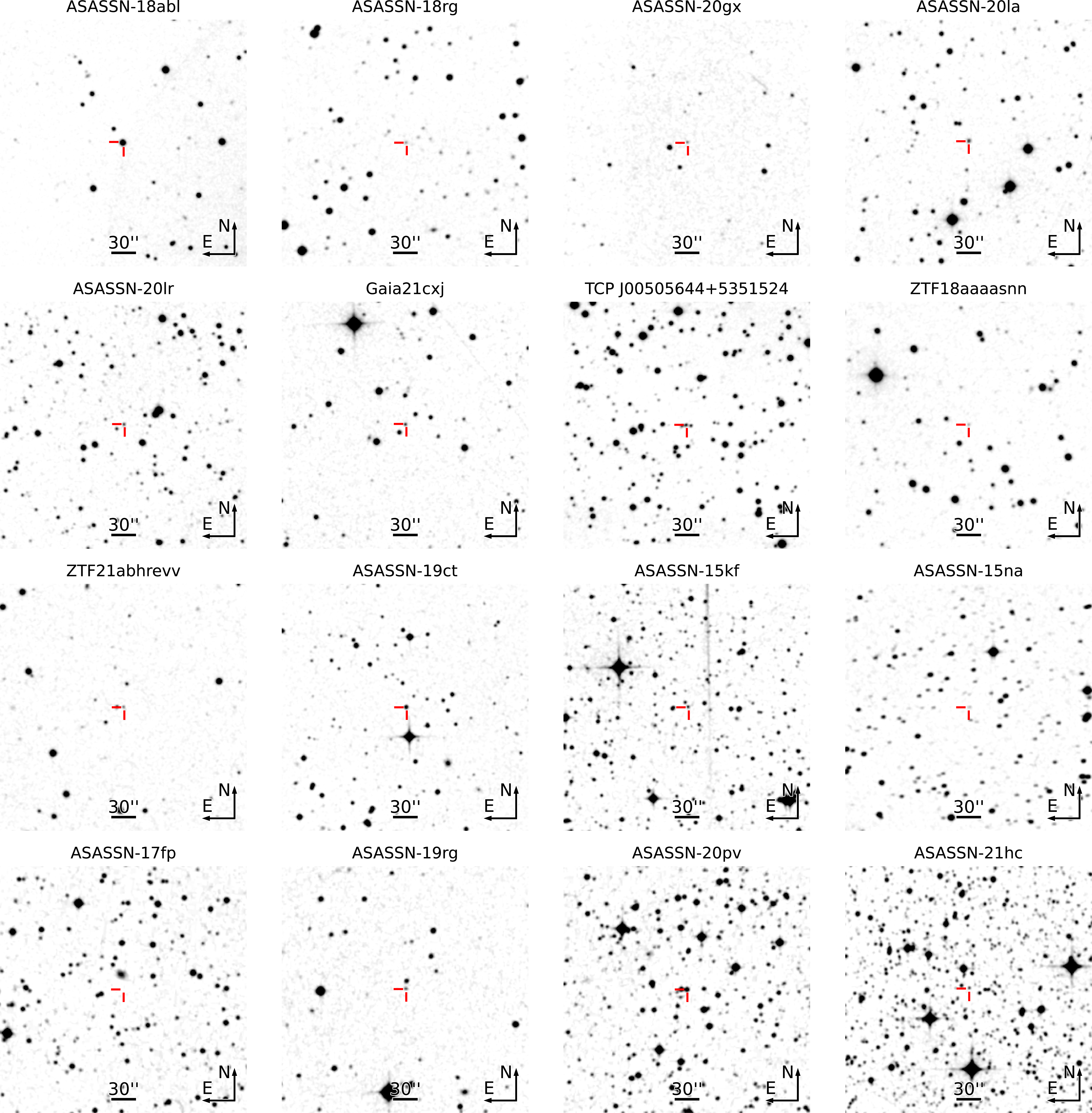
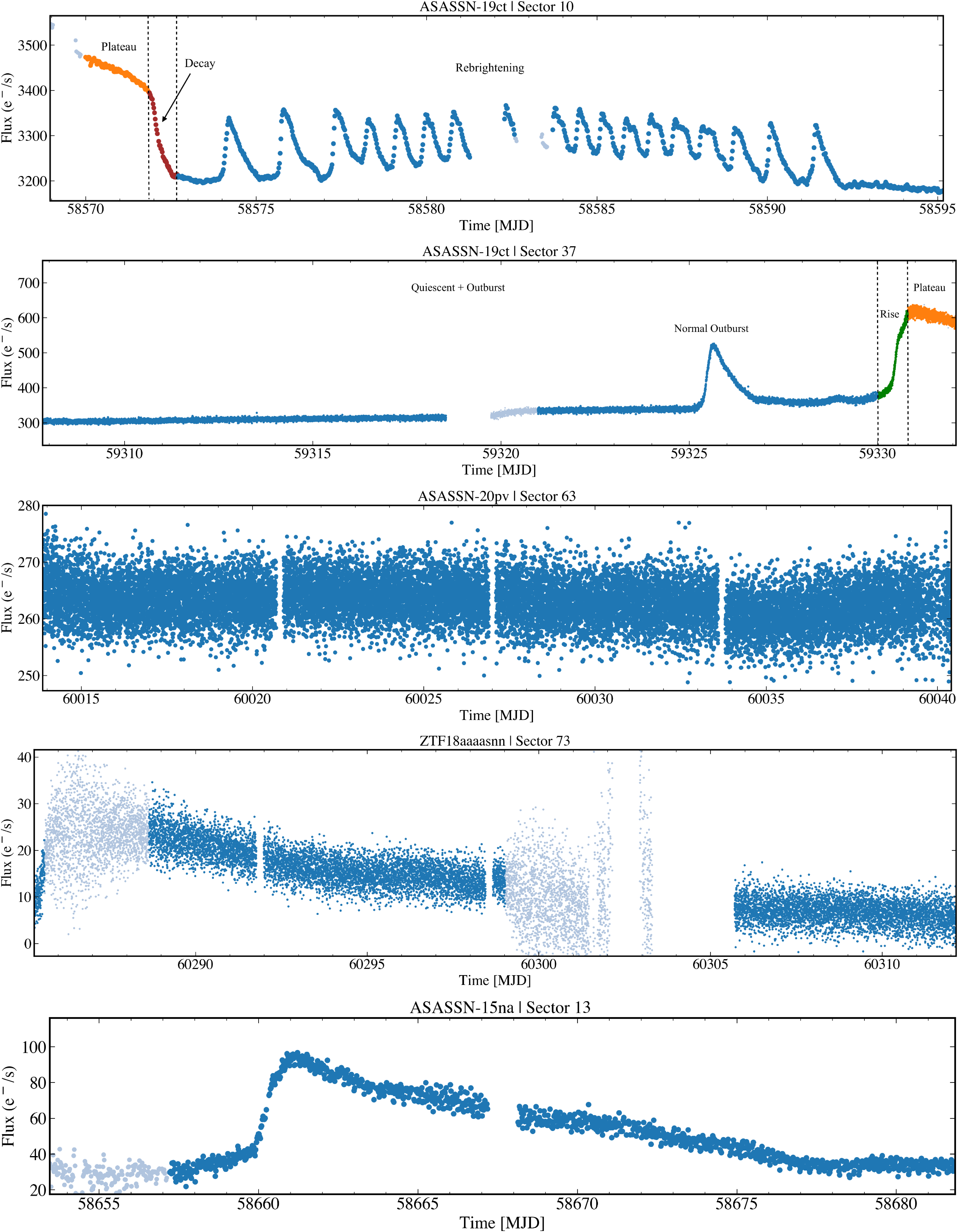
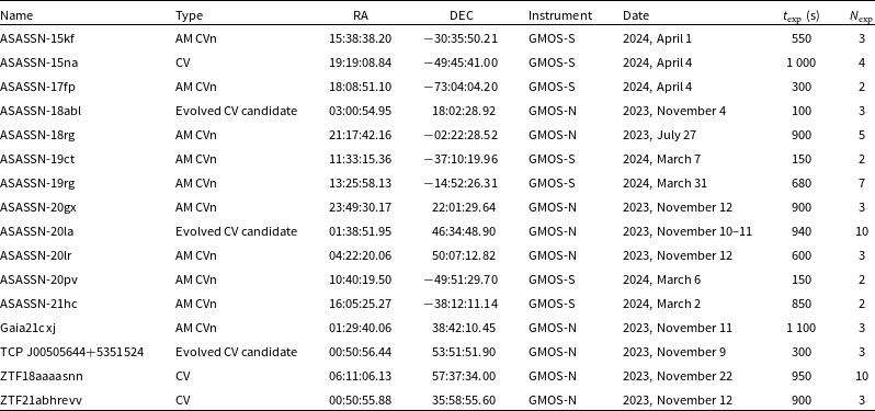


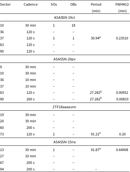
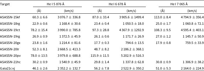
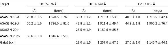
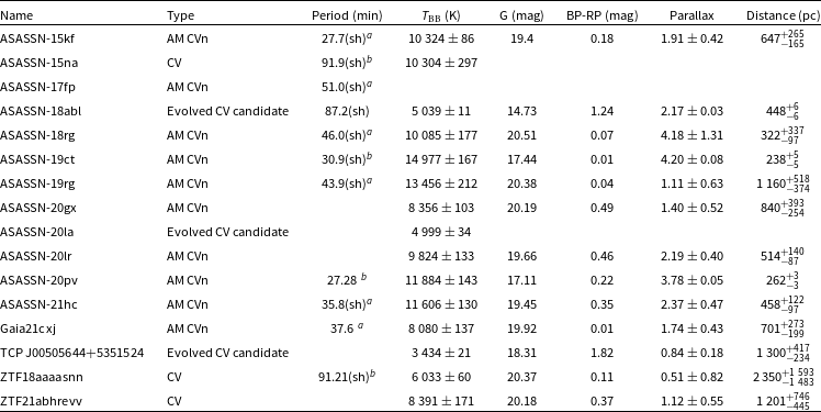
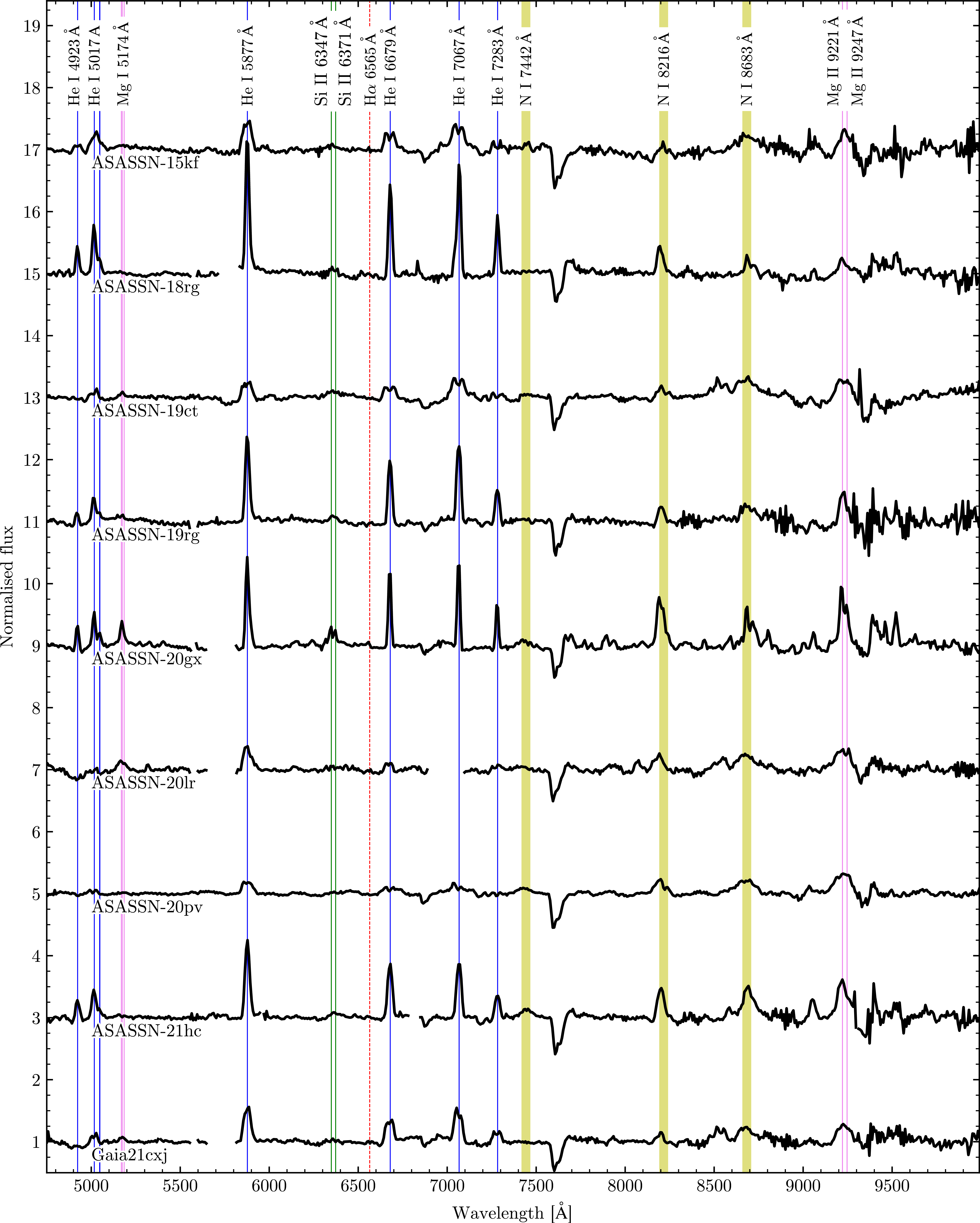

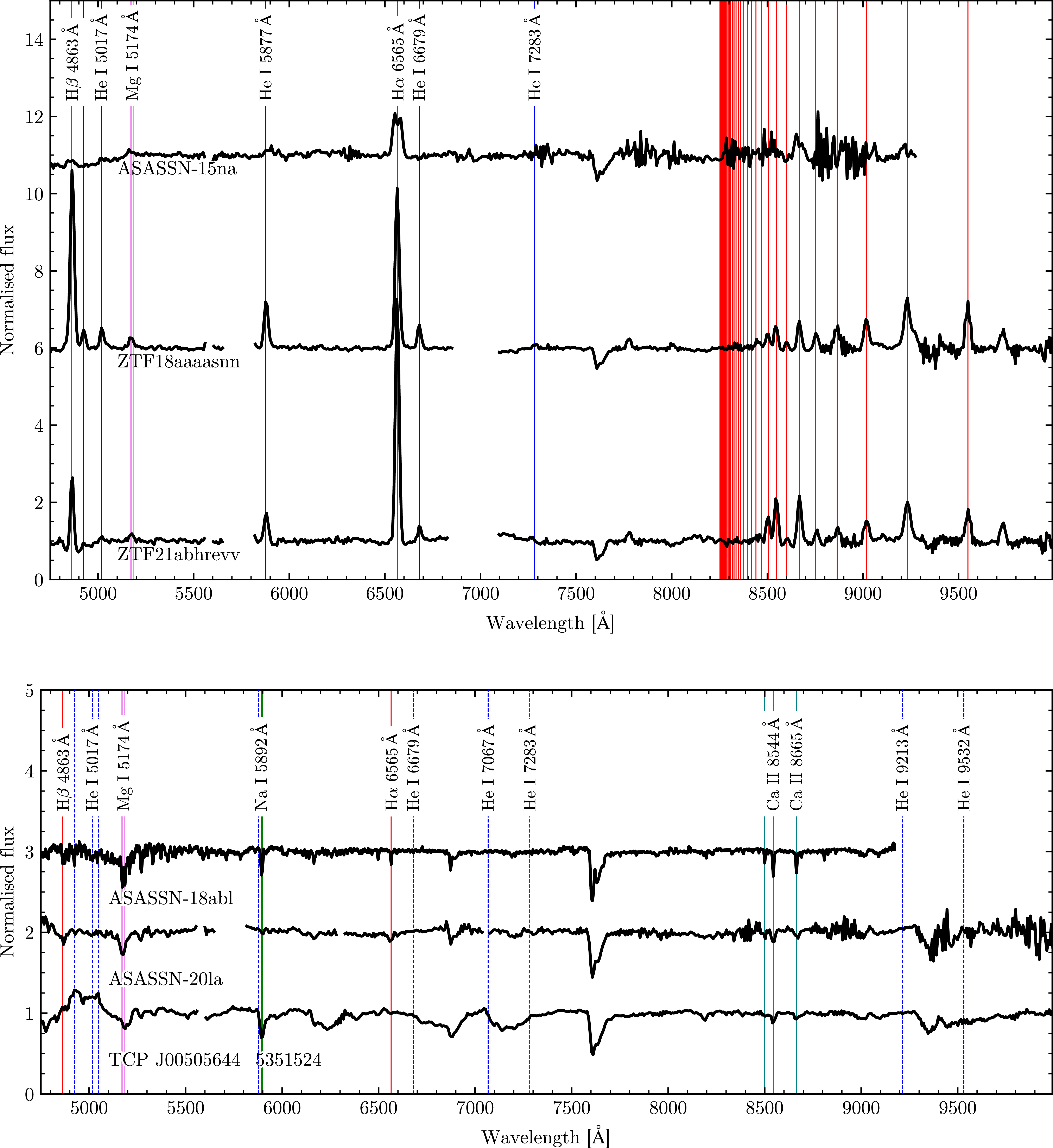

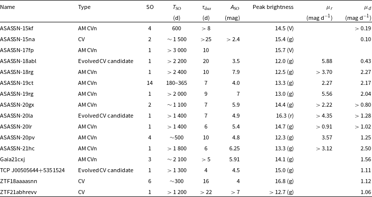


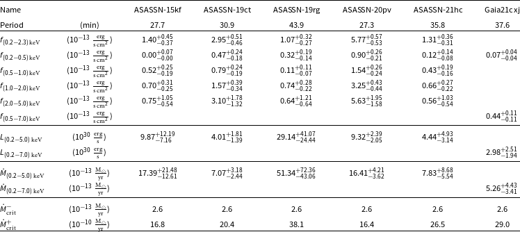


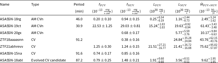
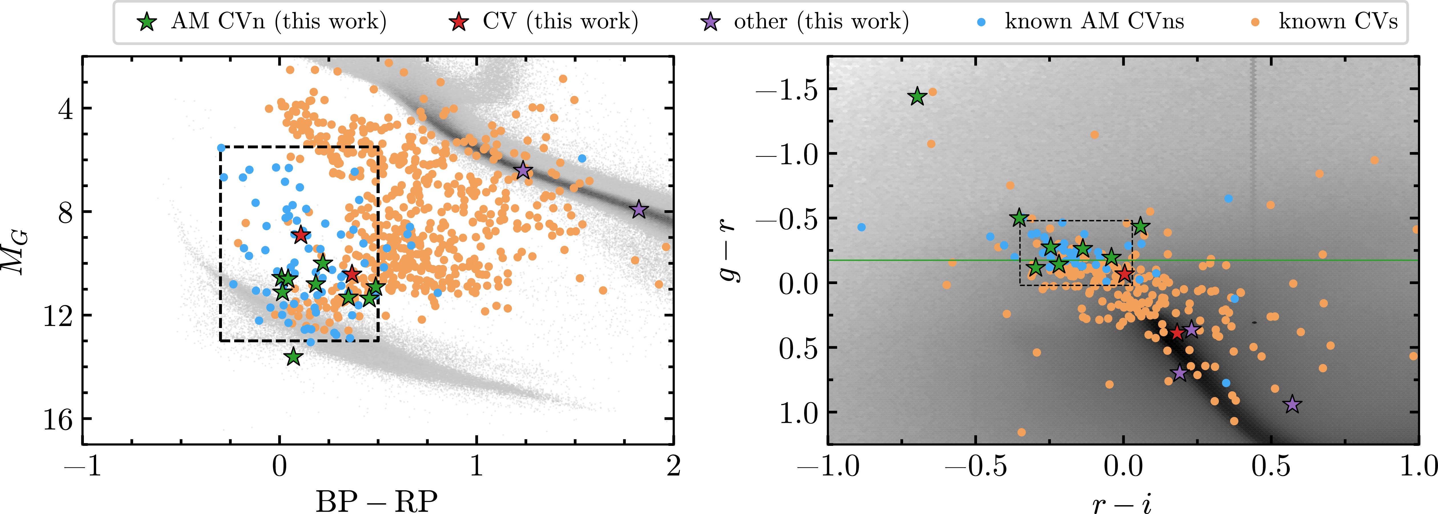
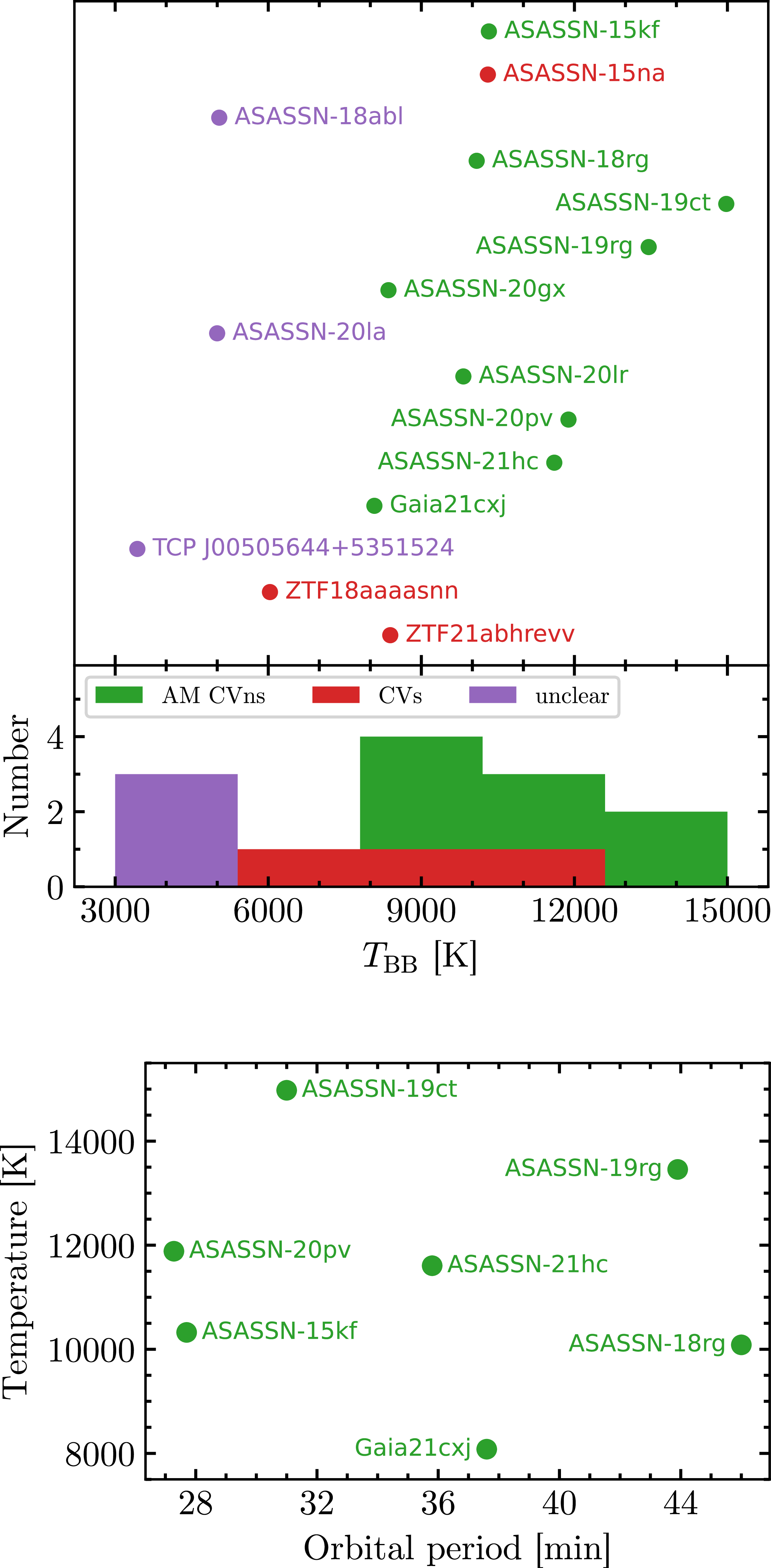
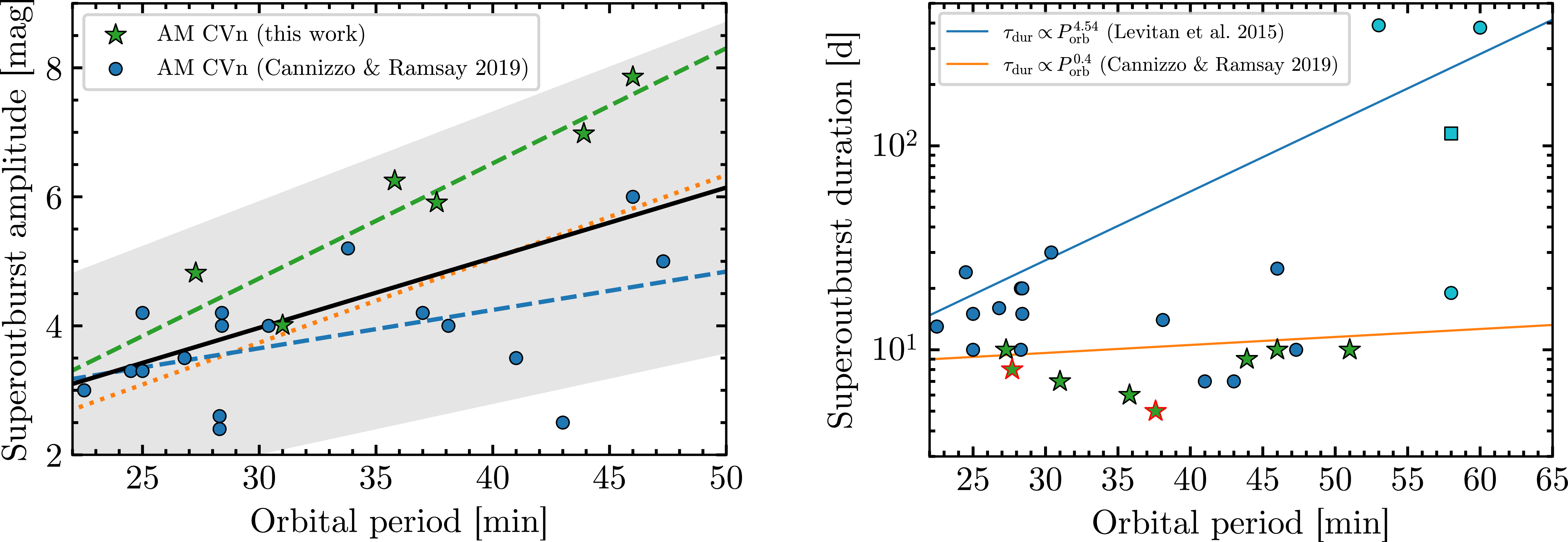


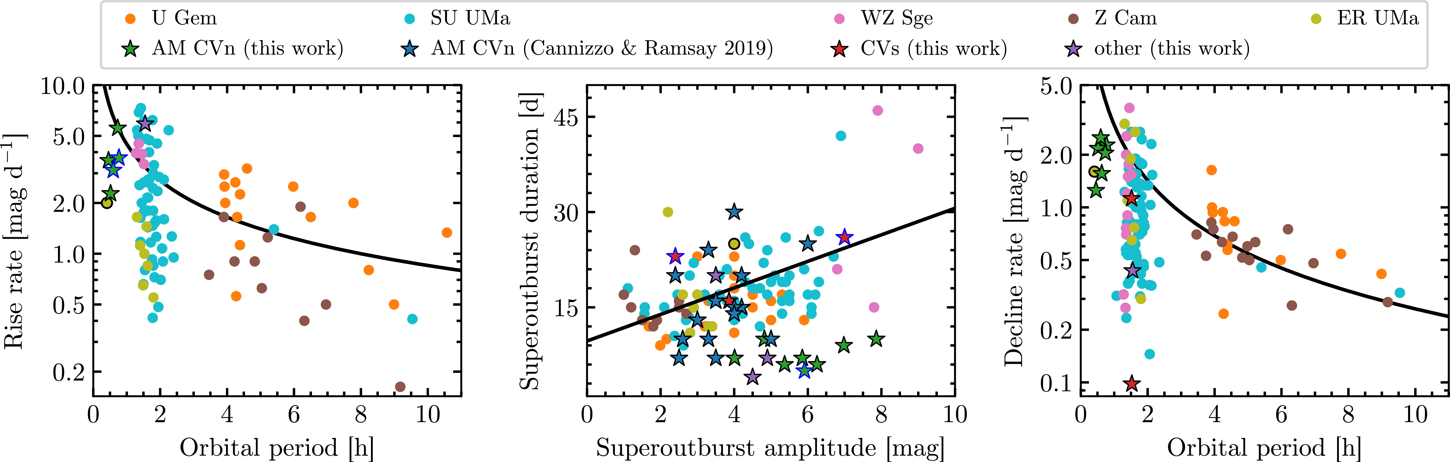
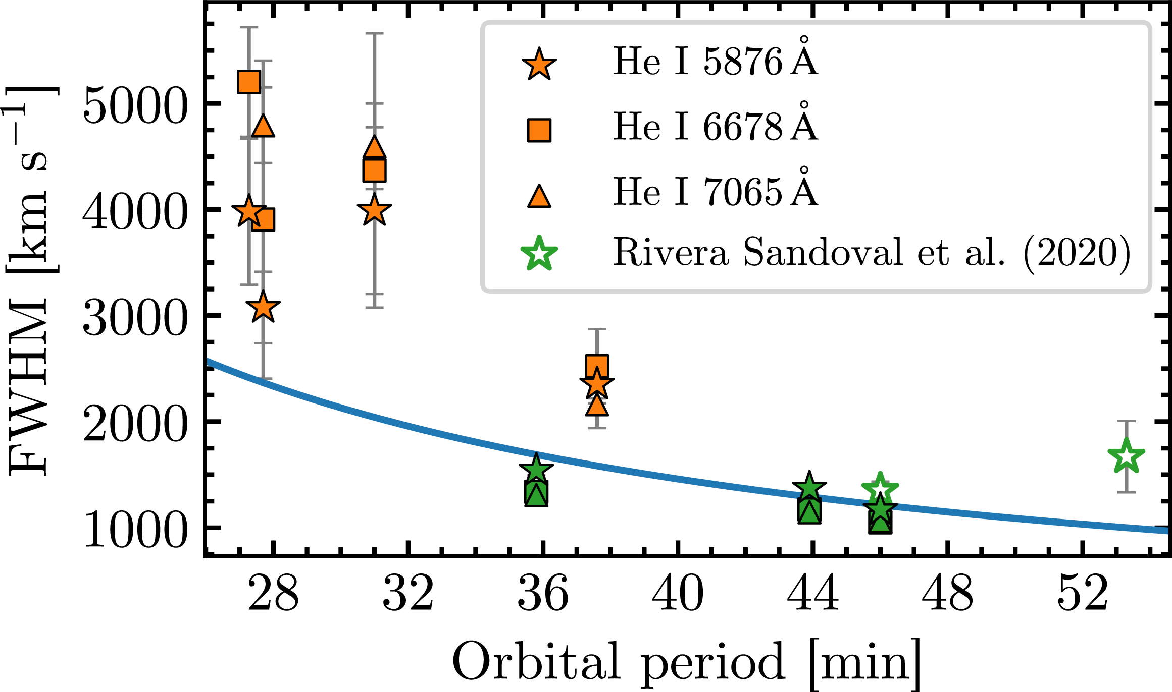
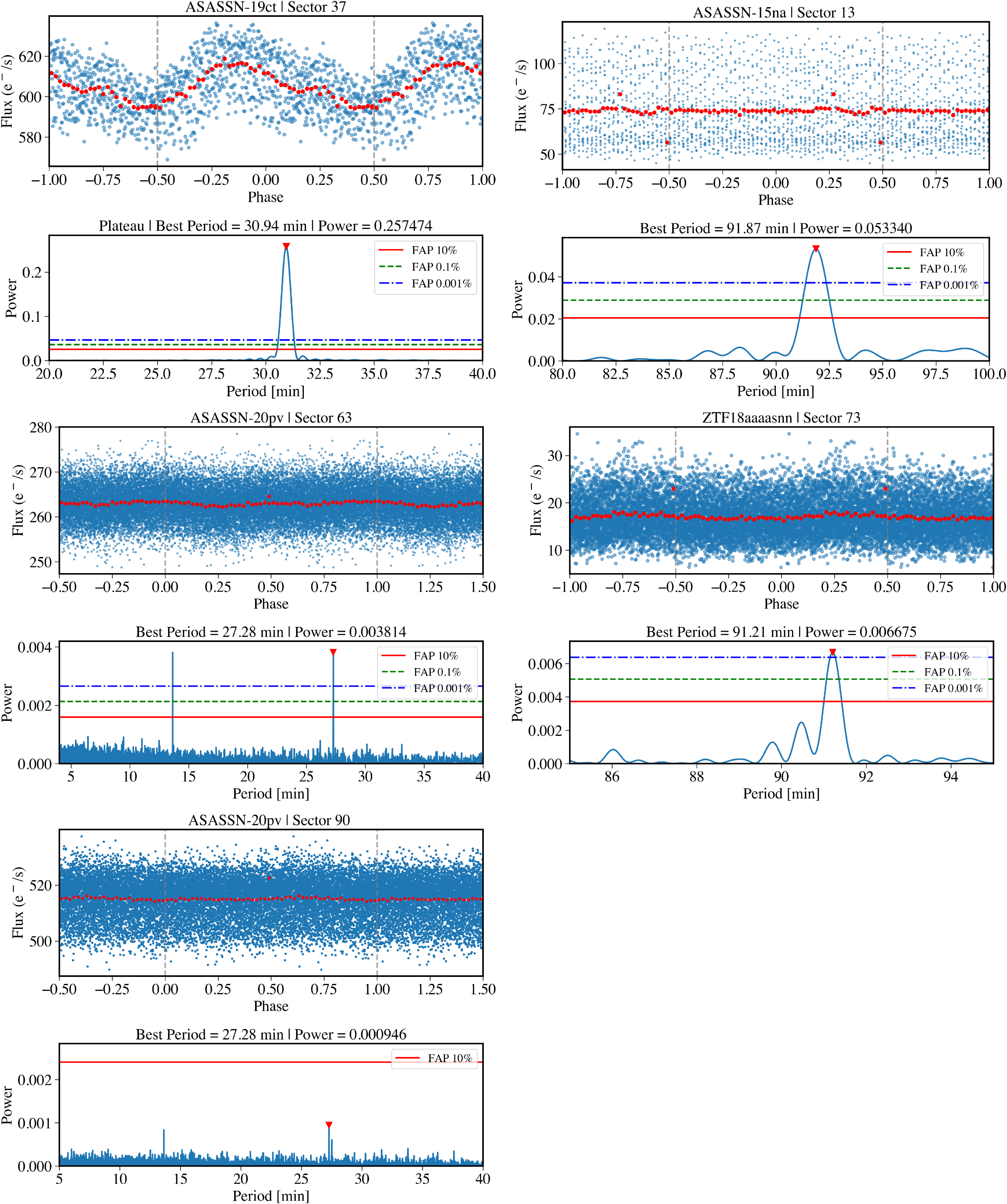

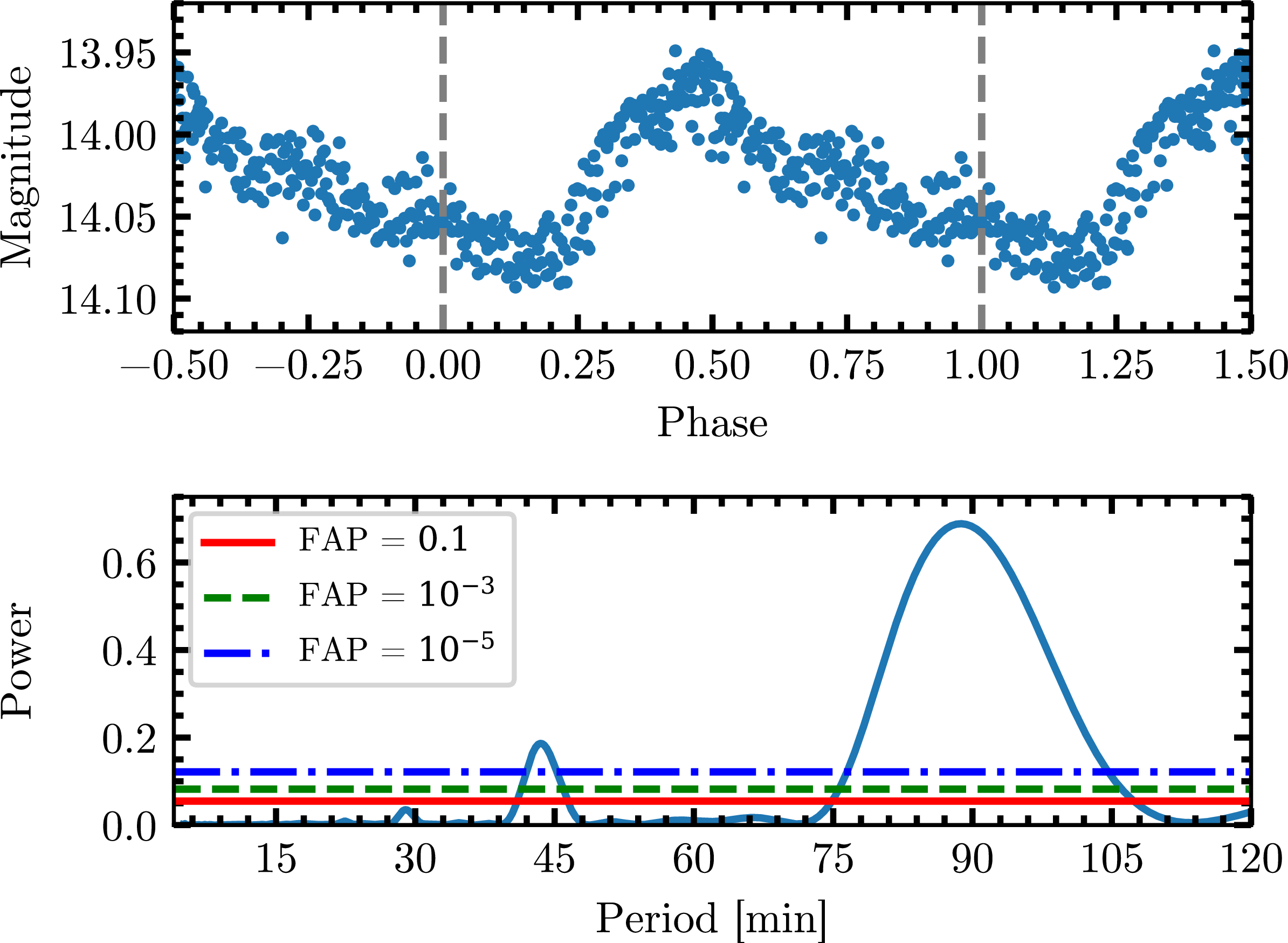


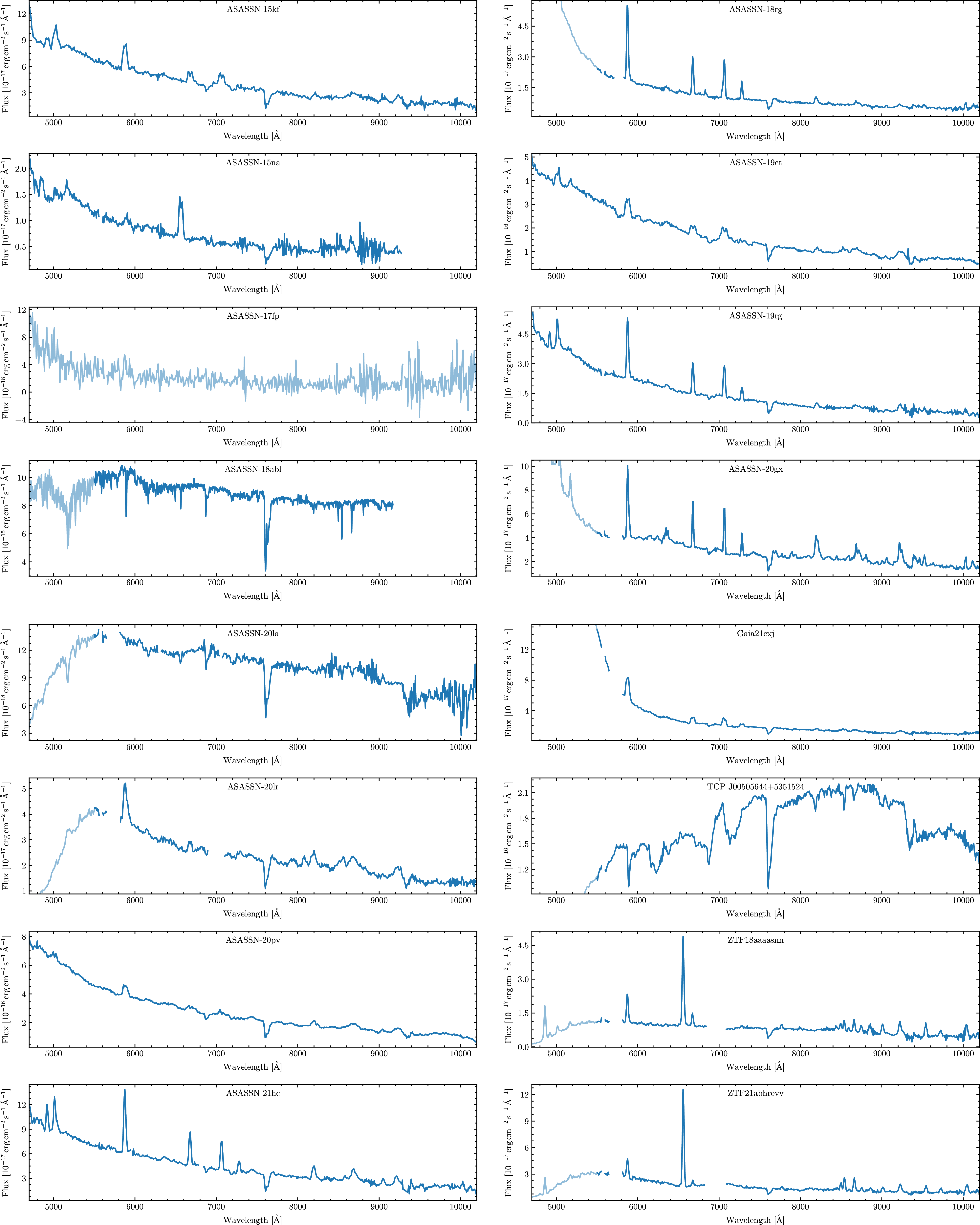
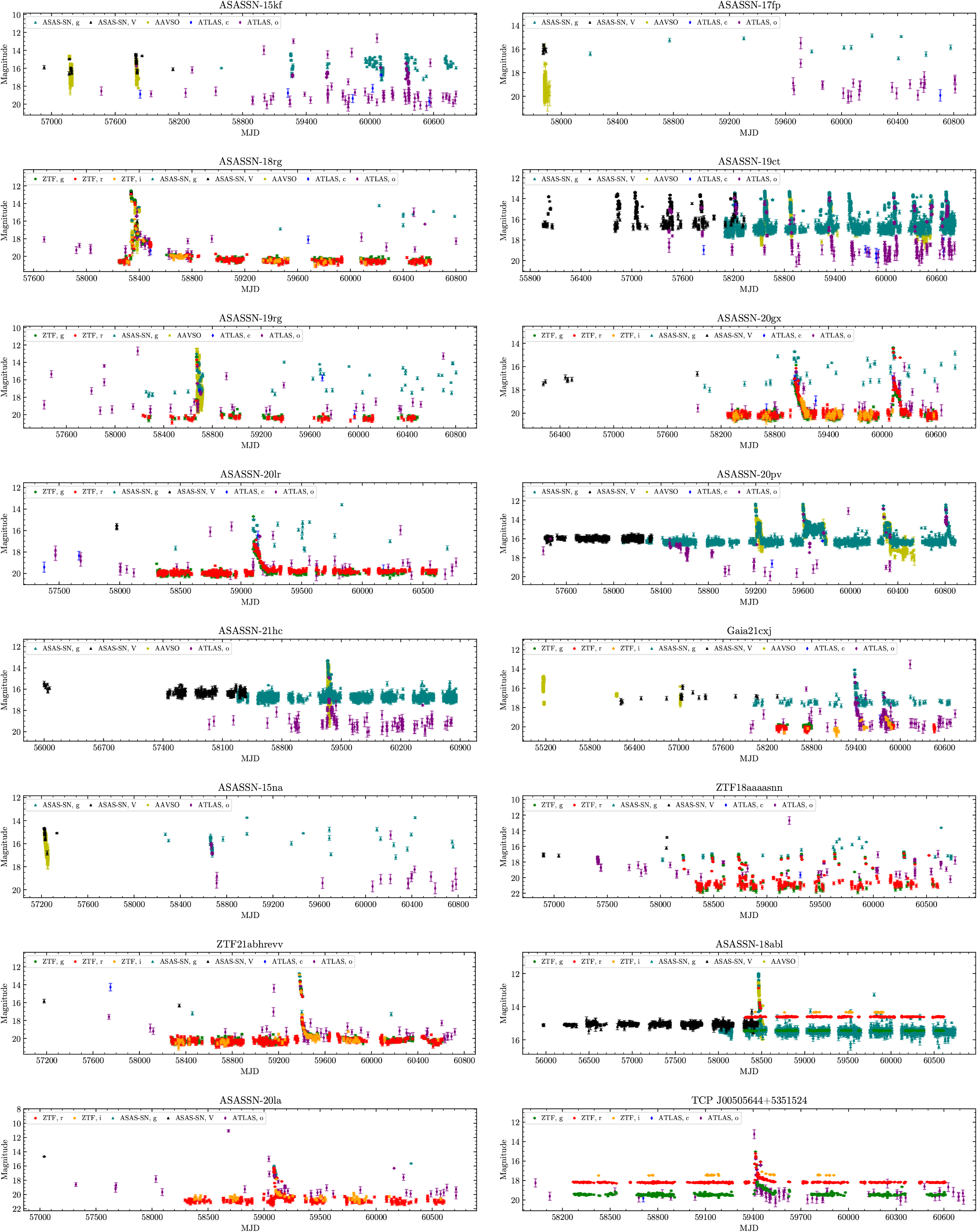

 Open access