


1. Introduction
As digital technology becomes integral to every facet of daily life, cyber risk has emerged as a critical global concern, underscoring the need for effective assessment to develop robust risk management strategies. Consequently, modeling of cyber risk has become a formidable scholarly challenge, driven by the increasing dependence on information technology and the rise of large-scale cyber attacks. Cyber risk was ranked as the top global risk in the Allianz Risk Barometer in 2024 (Allianz, 2024). According to the annual data breach report published by Ponemon Institute (2024), the global average cost of a data breach incident reached a historical high in 2024, with a 10% increase from 2023. PwC’s 26th Global Digital Trust Insights survey reports the global average cost of a damaging cyber-attack to be $4.4M (PricewaterhouseCoopers, 2024).
With the growing severity of cyber incidents comes an increasing demand for security solutions pertaining to the management of cyber risks. A widely accepted definition constructed by Cebula and Young (Reference Cebula and Young2010) defines cyber risks as operational risks that may result in potential violation of confidentiality, availability, or integrity of the information system. The formulation of viable and effective cyber risk management strategies requires a thorough understanding of the risk including both its arrival mechanism and statistical properties.
The detection and prediction of cyber attacks based on technical aspects have been studied extensively, primarily in the field of computer science and information technology. We refer readers to Sun et al. (Reference Sun, Zhang, Rimba, Gao, Zhang and Xiang2018), Husák et al. (Reference Husák, Komárková, Bou-Harb and Čeleda2018), and He et al. (Reference He, Jin and Li2024) for a comprehensive review of the topic. On the statistical side, stochastic processes have been prescribed for the study of cyber risk arrivals. Autoregressive conditional duration (ACD) processes were used by Peng et al. (Reference Peng, Xu, Xu and Hu2017) to model the arrival of extreme attack rates, while Xu et al. (Reference Xu, Schweitzer, Bateman and Xu2018) and Ma et al. (Reference Ma, Chu and Jin2022) used ACD processes to model inter-arrival times of data breach attacks. Autoregressive conditional moving average (ARMA) with generalized autoregressive conditional heteroskedasticity (GARCH) processes were proposed to model the evolution of breach sizes (Xu et al., Reference Xu, Schweitzer, Bateman and Xu2018; Ma et al., Reference Ma, Chu and Jin2022) or attack rates (Xu et al., Reference Xu, Hua and Xu2017; Peng et al., Reference Peng, Xu, Xu and Hu2018). Poisson processes were utilized by Zeller and Scherer (Reference Zeller and Scherer2022) to model the arrival of idiosyncratic and systemic events separately. Bessy-Roland et al. (Reference Bessy-Roland, Boumezoued and Hillairet2021) model the frequency of cyber attacks in the PRC data using a multivariate Hawkes process, a non-Markovian extension of the Poisson process with a mutual-excitation property, capturing both shocks and persistence aftershocks of an attack.
Among the literature using stochastic processes to study cyber risks, a stream of recent publications has employed epidemic processes to capture the underlying contagion mechanism of the risk. Fahrenwaldt et al. (Reference Fahrenwaldt, Weber and Weske2018) described the propagation of cyber infections with a susceptible-infected-susceptible (SIS) process within an undirected network. Their simulations revealed that the structure of the network was important both for the pricing of cyber insurance and the formulation of effective risk management strategies. An SIS process with non-zero exogenous infection rates was studied by Xu and Hua (Reference Xu and Hua2019), who used both Markov and non-Markov models to capture the transition between states and derive dynamic upper bounds for the infection probability. They also used copulas to model the joint survival function, thus capturing multivariate dependence among risks. Experiments on the Enron email network demonstrated that the recovery rate significantly influenced insurance premiums. Hillairet and Lopez (Reference Hillairet and Lopez2021) described the spread of a cyber attack at a global level with a susceptible-infected-recovered (SIR) process, and approximated the centered process of the cumulative number of individuals in each group with Gaussian processes. Continuing this work, Hillairet et al. (Reference Hillairet, Lopez, d’Oultremont and Spoorenberg2022) segmented the whole population into groups and incorporated digital dependence with a contagion matrix. Their simulation results showed that infection speed and final epidemic size in each sector are influenced by network connectivity patterns and group response strategies.
The statistical properties of cyber risks lie at the core of actuarial modeling of cyber losses, which usually takes a loss distribution approach (LDA) by describing the frequency and severity using separate models. Edwards et al. (Reference Edwards, Hofmeyr and Forrest2016) developed a Bayesian generalized linear model that incorporates a negative binomial prior distribution with a gamma-distributed skewness parameter and a time-varying location parameter to model data breach frequency, while severity was described by either a lognormal or a log-skew-normal model, acknowledging the heavy tail observed in data breach losses. Eling and Loperfido (Reference Eling and Loperfido2017), in their PRC data breach analysis, used a negative binomial distribution for loss frequency and lognormal or log-skew-normal distributions for the number of records lost in a data breach incident. They further applied multidimensional scaling to frequency and severity to investigate the difference in entities that experience data breaches and the difference between breach types. Woods et al. (Reference Woods, Moore and Simpson2021) aggregated individual parametric distributions into a county fair cyber loss distribution by averaging the optimal loss distributions using an iterative optimization process built on a particle swarm optimization of parameters of candidate loss distributions from insurance prices disclosed in regulatory filings of 26 insurers in California. Gamma distributions were discovered to be the most suited for predicting individual insurance liability prices.
Distributional analyses fall short of linking losses with explanatory factors. This limitation can be addressed by introducing regressions to model the distribution parameters. Eling and Wirfs (Reference Eling and Wirfs2019) focused on extreme losses and followed the dynamic extreme value theory (EVT) approach developed by Chavez-Demoulin et al. (Reference Chavez-Demoulin, Embrechts and Hofert2016). In their empirical study of the SAS OpRisk global dataset, they modeled frequency with a Poisson GLM and severity of extreme losses with a generalized Pareto distribution (GPD), whose parameters depend on the same set of regressors used previously. Their results supported the dynamic EVT approach over the traditional LDA. Malavasi et al. (Reference Malavasi, Peters, Shevchenko, Trück, Jang and Sofronov2022) also adopted a regression approach, but they generalized the GLM framework to the generalized additive models for location, shape, and scale (GAMLSS) pioneered by Rigby and Stasinopoulos (Reference Rigby and Stasinopoulos2005), allowing higher moments to be regressed on explanatory variables. Similar to Eling and Loperfido (Reference Eling and Loperfido2017), in their GAMLSS framework, a Poisson model for loss frequency and a GPD for severity were considered, for every risk category separately and for the entire data jointly. The authors further applied an ordinal regression framework to remove the scale of extreme cyber events. Their work on the Advisen cyber loss data found no significant distinction between a separate model for each risk type and a joint model, mainly driven by the existence of extreme events in the data. Unlike Eling and Wirfs (Reference Eling and Wirfs2019) and Malavasi et al. (Reference Malavasi, Peters, Shevchenko, Trück, Jang and Sofronov2022), Farkas et al. (Reference Farkas, Lopez and Thomas2021) built regression trees for both the central part of the PRC data and the right tail to fit and predict the conditional mean and median of the number of breached records in a cyber incident. The tail of the distribution was modeled by generalized Pareto regression trees. This work acknowledged the heterogeneity in cyber events and the heavy-tailedness of their resulting losses.
Despite theoretical progress in configuring a framework to describe the spread of cyber risks on the Internet, and a growing number of empirical papers exploring statistical models for the resulting losses, there is a lack of work that brings these two research streams together in the analysis. Our work seeks to bridge this gap by combining theoretical modeling of cyber risk propagation with empirical analysis of loss characteristics. Specifically, we contextualize the development in loss counts over time as a discrete-time SIR process within a complete network of infinite population and explore their relationship to covariates, while capturing the severity of each incident using regression models. Through modeling the transition rates between states with temporal and covariate dependence, we effectively remove the scaling effect caused by the size of the infectious population on the number of new infection counts per year, thereby describing the true underlying dynamics more accurately. Our simulations demonstrate that modeling cyber risks under the SIR framework can significantly enhance the accuracy of aggregate loss prediction, addressing both typical and average loss scenarios, as well as heavy right tails.
Our contributions to the literature are threefold. First, we bridge the gap between theoretical conjectures on the propagation of cyber risks and empirical studies by introducing a novel approach to quantifying cyber losses by framing the evolution of cyber incident counts within an SIR process. Unlike traditional LDA, which models frequency using standard count distributions or GLMs, we model loss frequency as an epidemic process governed by transmission and recovery rates, thus providing a more theoretically grounded and empirically robust framework for modeling cyber risk. Second, our methodology advances existing cyber risk models by incorporating a more flexible rate-based structure. We model the transition rates of the SIR process using both standard distributions and GAMLSS, allowing for richer dependency structures on time and covariates. We also address the challenge of incomplete demographic information by embedding the dependency on population size within time- and covariate-dependent transition rates, which can effectively internalize the impact of system-wide exposure into the modeling process, avoiding biases introduced by scaling effects, with sensitivity analysis confirming the robustness of the framework. These predicted transition rates help inform pricing by identifying periods of rising systemic risk that may justify surcharges or stricter terms and periods of decline that support more stable premiums. Finally, our empirical results demonstrate that even with time-varying parameters alone, our SIR-informed model delivers superior prediction accuracy compared to traditional LDA methods. This comparative analysis underscores the importance of incorporating epidemic-style dynamics into cyber risk models, paving the way for future research in this domain. Moreover, the findings hold significant relevance for actuarial applications in risk management and capital reserving, where accurate loss projections are crucial for decision-making.
The remainder of this paper is structured as follows. In Section 2, we introduce the dataset, define the theoretical framework describing the propagation process of the risk, and outline the regression approach applied to frequency, severity, and transition rate models. Section 3 presents results obtained using the LDA widely adopted in actuarial practice, where marginal frequency and severity models involve parametric distributions and generalized linear models (GLM), respectively. Section 4 extends Section 3 by recasting the development of infection and recovery counts in the context of an SIR model and modeling the movement of counts by modeling the underlying transition rates. Section 5 presents the application of the SIR-informed framework to aggregate loss simulation, comparing its performance with alternative frequency and severity models to derive insights for risk management decisions. Section 6 concludes the paper.
2. Data and methodology
In this section, we describe the dataset and the methodological framework utilized in this study. Subsection 2.1 provides an overview of the dataset, detailing the key variables available for analysis. In Subsection 2.2, we introduce the SIR epidemic process, which serves to model the dynamic trajectory of infection and recovery counts. Finally, Subsection 2.3 provides a detailed exposition on how the dataset is used to fit marginal models, incorporating both deterministic parameters and covariate-dependent parameters for frequency and severity distributions, as well as how the SIR framework is integrated to model the counts of cyber risk incidents.
2.1 Data
A total of 1,933 cyber incidents reported between January 1970 and November 2021 have been extracted from the SAS OpRisk Global Data, following the selection process proposed by Eling and Wirfs (Reference Eling and Wirfs2019). The dataset reports the first year and the last year of occurrence of the same security incident, as well as the industry, region, number of employees, and revenue size of the breached firm, the risk category, whether multiple firms are affected or multiple losses are observed, and the financial loss from the reported events. The set of feature names from the raw dataset that are used to construct the model covariates is listed in Table 1. Notably, approximately 73% of the reported cyber incidents originate from financial institutions, underscoring the prominence of this sector in the dataset. Geographically, the Americas record the highest number of incidents, accounting for 53% of the total reports, followed by Asia with 21%. Regarding risk categories, internal fraud emerges as the most prevalent, constituting 44% of incidents, while external fraud follows closely behind at 28%. Large firms, characterized by their number of employees, constitute 86% of the breached entities. Furthermore, almost 90% of incidents result in multiple losses, and 84% of incidents involve more than one firm, highlighting the interconnected nature of cyber threats. There are a few missing entries regarding the number of employees and the revenue size of breached firms, which are imputed using the K-Nearest Neighbors method (Cover & Hart, Reference Cover and Hart1967; Fix & Hodges, Reference Fix and Hodges1985).
Dataset feature names

In our regression analysis, we utilize the aforementioned firm- and incident-specific features available in the dataset. Several of these are categorical and are transformed into binary indicator variables before aggregation into annual time series by population group. In more detail, these features, integrated at the population level, recorded for every $t \in \{1970,1971,\ldots ,2020,2021\}$
(for every covariate, the subscript
$t \in \{1970,1971,\ldots ,2020,2021\}$
(for every covariate, the subscript $t$
representing the calendar year is omitted for simplicity), to fit the model include:
$t$
representing the calendar year is omitted for simplicity), to fit the model include:
-
• $F_i, i\in \mathcal{I}=\{\text{Financial Services (FS) or Information, non-FS and non-Information}\}$
, indicating the number of infectious individuals in each industry sector,
$F_i, i\in \mathcal{I}=\{\text{Financial Services (FS) or Information, non-FS and non-Information}\}$
, indicating the number of infectious individuals in each industry sector, -
•
$A_j, j \in \mathcal{J}=\{\text{Americas or Europe or Asia, Oceania and Africa}\}$
, indicating the number of losses recorded in each respective region, -
•
$C_k, k\in \mathcal{K}=$
{BS, FIP, DPA, EF, IF}, represents the number of incidents across five risk categories: Business Disruption and System Failures (BS), Failed Internal Processes (FIP), Damage to Physical Assets (DPA), External Fraud (EF), and Internal Fraud (IF). -
•
$E_l, l\in \mathcal{L}=\{\text{small to medium, large}\}$
, indicating the number of breached entities in the two classes of company sizes in terms of the number of employees. This grouping is based on the definition of small and medium-sized enterprises (SMEs) used in the European Union (Eurostat, 2022). -
•
$W_m, m\in \mathcal{M}=\{\text{small to medium, large}\}$
, indicating the number of breached entities in the two classes of company sizes in terms of revenue, -
•
$MF$
, indicating the number of incidents that affect multiple firms, -
•
$ML$
, indicating the number of incidents that incur multiple losses in the same firm.


The selection of covariates is motivated by Eling and Wirfs (Reference Eling and Wirfs2019) and Malavasi et al. (Reference Malavasi, Peters, Shevchenko, Trück, Jang and Sofronov2022). In the following models for frequency, severity, and transition rates under the epidemic framework, these features are consolidated into an $n \times k$
covariate matrix
$n \times k$
covariate matrix $\boldsymbol{X}$
, where
$\boldsymbol{X}$
, where $n$
is the number of observations and
$n$
is the number of observations and $k$
is the number of covariates used in the regression.
$k$
is the number of covariates used in the regression.
For counts modeling, we organize the data into a time series format according to the first and last year of incidence. Each incident can span multiple calendar years, likely due to continued operational disruption, extended investigation, or regulatory proceedings. We define the first year of occurrence as the start of infection, treat every subsequent year up to and including its last year of occurrence as an actively infectious period, and then classify the firm as recovered in the year following the last active year. Accordingly, we construct the infectious population by counting all incidents that are active in a given year, including both newly initiated and ongoing cases. The number of recovered firms in any year is defined as the total number of incidents that ended in the previous year or any year before that. It is worth noting that the state transitions are not meant to represent exact technical infection or remediation events, but the observable lifecycle of incidents as captured in public records. Similarly, the transmission and recovery rates do not imply direct contagion between firms, but rather serve as mechanisms to model the dynamics of incident counts over time using the epidemic-inspired structure. The transmission rate reflects the rate at which new incidents emerge among at-risk firms, and the recovery rate reflects the rate of infected firms exiting the actively infectious state, conditional on covariates. To build covariates at the population level, we compute group-level totals of firm- and incident-specific characteristics separately for the infectious and recovered groups. Since these features are one-hot encoded as indicator variables, the yearly totals represent the number of active incidents associated with each characteristic. This aggregation ensures consistency between population states and explanatory variables, enabling a structured translation of incident-level data into annual time series aligned with the SIR model framework.
To provide context for the modeling framework, we first summarize the key features of the infection and recovery time series. Annual new infection counts range from 0 to 144 per year, while annual recovery counts range from 0 to 146. The early years show a low volume of reports, with a noticeable increase in activity beginning in the late 1990s. Of the 52 calendar years, 26 have no recorded recoveries, and 11 have zero infection counts. While these zero values are more common in the early part of the series, they also occur intermittently in later years. The frequency of zero values across the time series motivates the use of zero-inflated count models in the regression analysis. Both infection and recovery counts peak in the late 2000s, followed by a sharp decline in infection counts and a more fluctuating trend in recovery counts post-peak. Given the limited size of the dataset, our capacity to assess stationarity, seasonality, or autocorrelation structure in the data is constrained. Thus, instead of time series models, we use regression models that do not rely on these assumptions, meanwhile compensating for the lack of temporal depth with covariate-driven analysis.
Figure 1 displays the distribution of annual infection and recovery counts. Both are right-skewed with abundant small values. Figure 2 summarizes how the new infection counts vary when grouped by region, risk category, industry, and company size by the number of employees. The number of annual infections in the Americas displays a significantly broader spread and higher median compared to other regions. Both external and internal frauds (risk category EF and IF, respectively) demonstrate higher medians and wider spreads than other risk categories, highlighting the impact of human factors in cyber infection. In terms of industry, organizations providing financial services exhibit the widest range and highest median, largely surpassing even the second most prominent sector, the information industry. Large companies (with more than 250 employees) constitute the majority of observations and show the widest span with the highest median. These notable variations within each grouping suggest that region, risk category, industry, and company size may play significant roles in infection counts and rates models. These findings signal that firm- and incident-specific features might be important risk factors for predicting cyber infection counts, hence are utilized in the regression analysis.
Histograms of new infection and recovery counts per year.

Boxplot of new infection counts by region (top left), risk category (top right), industry (bottom left), and company size according to number of employees (bottom right).

Boxplots of the logarithm of losses using a sliding window of a year are shown in Figure 3. There is noticeable variation in the median and the variance across the years, whilst no lasting trend could be identified. Moreover, large losses are more frequently observed in events that first occurred around the early 2000s. We also explore the variation in the log of loss severity with respect to region, risk category, industry, and company size groups, illustrated in Figure 4. Unlike the clear distinction in the infection counts, little variation was observed across different regions, and slightly more variation across industries and company sizes. Variation across risk categories stands out as the most prominent, with DPA and business disruption and system failure (BS) resulting in the highest median losses among all risk types.
Boxplot of log(loss) by the first year of incident occurrence.

Boxplot of loss severity by region (top left), risk category (top right), industry (bottom left), and company size according to number of employees (bottom right).

With an understanding of the data structure and key features available for analysis, we next introduce the SIR model framework in Subsection 2.2. Given the complex dynamics of cyber risk propagation, the SIR model serves as a foundational approach to mimic infection and recovery processes. We explore several extensions of the basic SIR model, including time-varying, age-dependent, and covariate-driven structures, to capture more nuanced patterns in our data.
2.2 Discrete-time SIR model
The classical discrete-time SIR model, characterized by constant transmission and recovery rates within a fully connected network, is governed by the following set of equations:
 \begin{align*} S(t+1) &= S(t)- \beta \frac {S(t)I(t)}{N}, \\ I(t+1) &= I(t) + \beta \frac {S(t)I(t)}{N} -\gamma I(t),\\ R(t+1) &= R(t)+\gamma I(t), \end{align*}
where $S(t)$
,
$S(t)$
, $I(t)$
and
$I(t)$
and $R(t)$
are the number of susceptible, infected, and recovered nodes at time
$R(t)$
are the number of susceptible, infected, and recovered nodes at time $t$
, respectively,
$t$
, respectively, $0\lt \beta \lt 1$
and
$0\lt \beta \lt 1$
and $0\lt \gamma \lt 1$
are the rates of transmission and recovery, respectively, and
$0\lt \gamma \lt 1$
are the rates of transmission and recovery, respectively, and $N$
is the size of population which is assumed to be fixed throughout (Allen, Reference Allen1994; Wacker & Schlüter, Reference Wacker and Schlüter2020).
$N$
is the size of population which is assumed to be fixed throughout (Allen, Reference Allen1994; Wacker & Schlüter, Reference Wacker and Schlüter2020). $\beta$
represents the probability per unit time that a susceptible individual comes into contact with an infected one and becomes infected, and
$\beta$
represents the probability per unit time that a susceptible individual comes into contact with an infected one and becomes infected, and $\gamma$
represents the probability per unit time that an infected individual recovers. Given that organizations may experience more cyber incidents in the future, recovery is best conceptualized not as permanent immunity, but as a removal from the current infectivity pool. Recovered organizations have resolved a breach and are no longer actively contributing to the spread or growth of breaches, regardless of their future susceptibility. While reinfection is possible, it is relatively rare in our data, with less than 10% of reported incidents involving firms that have previously appeared in the dataset. We therefore do not explicitly model the reinfection process or temporary immunity, as these dynamics are highly heterogeneous and not directly observable. The SIR framework offers a parsimonious structure that captures the key observable transitions between infection and recovery.
$\gamma$
represents the probability per unit time that an infected individual recovers. Given that organizations may experience more cyber incidents in the future, recovery is best conceptualized not as permanent immunity, but as a removal from the current infectivity pool. Recovered organizations have resolved a breach and are no longer actively contributing to the spread or growth of breaches, regardless of their future susceptibility. While reinfection is possible, it is relatively rare in our data, with less than 10% of reported incidents involving firms that have previously appeared in the dataset. We therefore do not explicitly model the reinfection process or temporary immunity, as these dynamics are highly heterogeneous and not directly observable. The SIR framework offers a parsimonious structure that captures the key observable transitions between infection and recovery.
Instead, we focus on the changes in the sizes of the infected and recovered populations over time. We define the incremental changes in these two groups through the following system of difference equations:
 \begin{align*} \Delta I(t) & := I(t+1) - I(t) = \frac {\beta S(t)I(t)}{N} - \gamma I(t),\\ \Delta R(t) & := R(t+1) - R(t) =\gamma I(t). \end{align*}
Although the total population size $N$
is unknown in our dataset, since it is sufficiently large relative to the number of victimized entities, it is reasonable to assume
$N$
is unknown in our dataset, since it is sufficiently large relative to the number of victimized entities, it is reasonable to assume $\frac {S(t)}{N} \approx 1$
(Carpio & Pierret, Reference Carpio and Pierret2022), which leads to a linear approximation of the SIR process akin to a branching process (Allen, Reference Allen2017). This assumption affects only the transmission rate, as recovery is independent of the susceptible pool. To quantify the error introduced by this approximation, we later perform a sensitivity analysis by varying
$\frac {S(t)}{N} \approx 1$
(Carpio & Pierret, Reference Carpio and Pierret2022), which leads to a linear approximation of the SIR process akin to a branching process (Allen, Reference Allen2017). This assumption affects only the transmission rate, as recovery is independent of the susceptible pool. To quantify the error introduced by this approximation, we later perform a sensitivity analysis by varying $S(t)/N$
through alternative specifications of
$S(t)/N$
through alternative specifications of $N$
(see Section 4.3). Such discrete-time constant-parameter SIR processes with initial populations
$N$
(see Section 4.3). Such discrete-time constant-parameter SIR processes with initial populations $I_0$
and
$I_0$
and $R_0$
in the infected and recovered groups, constant transmission and recovery rates
$R_0$
in the infected and recovered groups, constant transmission and recovery rates $\beta$
and
$\beta$
and $\gamma$
, and the assumption that
$\gamma$
, and the assumption that $\frac {S(t)}{N} \approx 1$
can be solved analytically as follows,
$\frac {S(t)}{N} \approx 1$
can be solved analytically as follows,
 \begin{align} I(t) &= (1+\beta -\gamma )^t I_0, \end{align}
 \begin{align} R(t) &= R_0+\gamma I_0 \frac {1-(1+\beta -\gamma )^{t}}{\gamma -\beta }. \end{align}
As seen in Equations (2.2) and (2.3), without information on the susceptible population, the infected group size exhibits geometric growth. However, the linear approximation of transition rates works well only in the exponential growth phase of an outbreak; the impact of a changing susceptible population on the size of the infectious group at later stages cannot be effectively reflected. Additionally, the transition rates could vary with time due to factors such as the evolution of cyber defense technology and increasing connectivity in cyberspace. To address these limitations, it is essential to incorporate temporal variation in the transition rates. Allowing for time variation transforms the system dynamics to:
 \begin{align} \Delta I(t) &= \beta (t) I(t) -\gamma (t) I(t), \end{align}
 \begin{align} \Delta R(t) &= \gamma (t) I(t), \end{align}
which inherently models the quantity $\frac {S(t)}{N}$
in the estimation of the time-varying rates, and includes the constant parameter model as a special case. However, this time-varying extension lacks an explicit analytical solution. To express Equations (2.4) and (2.5) in matrix form, we let
$\frac {S(t)}{N}$
in the estimation of the time-varying rates, and includes the constant parameter model as a special case. However, this time-varying extension lacks an explicit analytical solution. To express Equations (2.4) and (2.5) in matrix form, we let $\boldsymbol{\Delta }(t):= \big ( \Delta I(t), \Delta R(t) \big )^\intercal$
be the column vector of the number of newly infected and newly recovered individuals between
$\boldsymbol{\Delta }(t):= \big ( \Delta I(t), \Delta R(t) \big )^\intercal$
be the column vector of the number of newly infected and newly recovered individuals between $t$
and
$t$
and $t+1$
,
$t+1$
,
 \begin{align} \boldsymbol{\Delta } (t) = \begin{pmatrix} I(t) & -I(t) \\ 0 & I(t) \end{pmatrix} \begin{pmatrix} \beta (t) \\ \gamma (t) \end{pmatrix} = \boldsymbol{\Phi }(t) \boldsymbol{\theta }(t), \end{align}
where $\boldsymbol{\Phi }(t):= \begin{pmatrix} I(t) & - I(t) \\ 0 & I(t) \end{pmatrix}$
, and
$\boldsymbol{\Phi }(t):= \begin{pmatrix} I(t) & - I(t) \\ 0 & I(t) \end{pmatrix}$
, and $\boldsymbol{\theta }(t)$
denotes the column vector of time-varying transition rates at time
$\boldsymbol{\theta }(t)$
denotes the column vector of time-varying transition rates at time $t$
.
$t$
.
Further incorporating the dependence of transmission and recovery rates on the infection age, similar to Kermack and McKendrick (Reference Kermack and McKendrick1927), leads to
 \begin{align*} \Delta I(t) &= \sum _{d=0}^w \beta (t,d) I(t,d) -\sum _{d=0}^w \gamma (t,d) I(t,d),\\ \Delta R(t) &= \sum _{d=0}^w \gamma (t,d) I(t,d), \end{align*}
where $I(t,d)$
with
$I(t,d)$
with $\sum _{d=0}^w I(t,d)=I(t)$
denotes the number of infectious nodes at time
$\sum _{d=0}^w I(t,d)=I(t)$
denotes the number of infectious nodes at time $t$
that are aged
$t$
that are aged $d$
,
$d$
, $w$
is the largest age of infection,
$w$
is the largest age of infection, $\beta (t,d)$
and
$\beta (t,d)$
and $\gamma (t,d)$
are transmission and recovery rates at age
$\gamma (t,d)$
are transmission and recovery rates at age $d$
at time
$d$
at time $t$
, respectively. To reduce the complexity of the system, we assume a separate age effect and a temporal effect, such that
$t$
, respectively. To reduce the complexity of the system, we assume a separate age effect and a temporal effect, such that $\beta (t,d)=\epsilon ^\beta _t+\upsilon ^\beta _d$
, where
$\beta (t,d)=\epsilon ^\beta _t+\upsilon ^\beta _d$
, where $\epsilon ^\beta _t$
and
$\epsilon ^\beta _t$
and $\upsilon ^\beta _d$
are function components that depend solely on time and infection ages, respectively. Likewise,
$\upsilon ^\beta _d$
are function components that depend solely on time and infection ages, respectively. Likewise, $\gamma (t,d)=\epsilon ^\gamma _t+\upsilon ^\gamma _d$
. With such assumptions,
$\gamma (t,d)=\epsilon ^\gamma _t+\upsilon ^\gamma _d$
. With such assumptions,
 \begin{align*} \Delta I(t) &= \epsilon ^\beta _t I(t) + \sum _{d=0}^w \upsilon ^\beta _d I(t,d) - \epsilon ^\gamma _t I(t) -\sum _{d=0}^w \upsilon ^\gamma _d I(t,d),\\ \Delta R(t) &= \epsilon ^\gamma _t I(t) + \sum _{d=0}^w \upsilon ^\gamma _d I(t,d). \end{align*}
The system of equations above can be expressed in a matrix form:
 \begin{equation} \boldsymbol{\Delta }(t) = \begin{pmatrix} I(t)\;\;\;\; & \mathbf{I}(t,d)\;\;\;\; & -I(t)\;\;\;\; & -\mathbf{I}(t,d) \\ 0\;\;\;\; & \mathbf{0}_{1\times w}\;\;\;\; & I(t)\;\;\;\; & \mathbf{I}(t,d) \end{pmatrix} \begin{pmatrix} \epsilon ^\beta _t \\ \boldsymbol{\upsilon }^\beta \\ \epsilon ^\gamma _t \\ \boldsymbol{\upsilon }^\gamma \end{pmatrix} = \boldsymbol{\Phi }(t,d) \boldsymbol{\theta }(t,d), \end{equation}
where $\mathbf{I}(t,d)$
is a row vector with
$\mathbf{I}(t,d)$
is a row vector with $w$
entries representing the number of infected individuals with infection age
$w$
entries representing the number of infected individuals with infection age $d$
at time
$d$
at time $t$
,
$t$
, $\boldsymbol{\upsilon }^\beta = (\upsilon _1^\beta ,\upsilon _2^\beta ,\ldots ,\upsilon _w^\beta )^\intercal \text{ and }\boldsymbol{\upsilon }^\gamma =(\upsilon _1^\gamma ,\upsilon _2^\gamma ,\ldots ,\upsilon _w^\gamma )^\intercal$
are column vectors of age-dependent components, and
$\boldsymbol{\upsilon }^\beta = (\upsilon _1^\beta ,\upsilon _2^\beta ,\ldots ,\upsilon _w^\beta )^\intercal \text{ and }\boldsymbol{\upsilon }^\gamma =(\upsilon _1^\gamma ,\upsilon _2^\gamma ,\ldots ,\upsilon _w^\gamma )^\intercal$
are column vectors of age-dependent components, and $\boldsymbol{\theta }(t,d)=(\epsilon _t^\beta ,\boldsymbol{\upsilon }^\beta ,\epsilon _t^\gamma ,\boldsymbol{\upsilon }^\gamma )^\intercal$
is the vector of temporal and age-dependent parameters.
$\boldsymbol{\theta }(t,d)=(\epsilon _t^\beta ,\boldsymbol{\upsilon }^\beta ,\epsilon _t^\gamma ,\boldsymbol{\upsilon }^\gamma )^\intercal$
is the vector of temporal and age-dependent parameters.
Having established the basis for modeling infection and recovery counts with the SIR model, we outline our broader modeling framework in Subsection 2.3. The framework enables a comparative analysis between models based on standard parametric distributions, GLM, and the SIR process. By juxtaposing these methods, we aim to assess the relative strengths of each in accurately modeling and predicting cyber risk.
2.3 Model framework
We adopt LDA, a traditional actuarial method that integrates independent models for frequency and severity, to model total losses by year. We use both standard probability distributions and GLM in which the responses depend on covariates as the marginal models. Besides modeling risk frequency, which is the number of new infection counts per year, we further conduct a distributional analysis and a GLM regression analysis on the annual new recovered counts, to investigate its statistical properties and identify its key risk drivers, in order to gain insights into the recovery process, in the hope of enabling more effective risk management and tailored insurance solutions.
In the standard distributional approach, Poisson and negative binomial distributions are commonly used in the literature to describe frequency (Edwards et al., Reference Edwards, Hofmeyr and Forrest2016; Eling & Loperfido, Reference Eling and Loperfido2017; Eling & Wirfs, Reference Eling and Wirfs2019; Malavasi et al., Reference Malavasi, Peters, Shevchenko, Trück, Jang and Sofronov2022), while the negative binomial distribution is often favored as it deals with skewness and heavy tails better than the Poisson distribution (see Appendix A for more details on these distributions). Because the data at hand exhibits a large number of zero infection and recovery counts, as observed in Figure 1, primarily due to rare reports in the early years, zero-inflated Poisson and negative binomial frequency distributions are also taken into consideration. With respect to severity models, standard continuous distributions with non-negative support are often used, such as exponential, generalized Pareto, generalized beta of the second kind (GB2), and its nested distributions, including gamma, lognormal, Weibull, and Burr type XII (see Appendix B for more details on severity distributions). Since the sample is strongly positively skewed with abundant small losses and a long right tail, we additionally consider modeling the body and the right tail separately with a peaks-over-threshold (POT) approach that assumes a GPD above a threshold (Balkema & De Haan, Reference Balkema and De Haan1974; Pickands, Reference Pickands1975), which is selected through maximizing the log-likelihood.
Standard distributions can only capture a static snapshot of the data, whereas GLMs can incorporate the dynamic change in the mean parameter over key risk factors. In Section 3.2, we utilize the firm- and incident-specific features available in the dataset, which are consolidated into the covariate matrix $\boldsymbol{X}$
. Results in Section 3.1 favor the negative binomial distribution for modeling infection and recovery counts due to its adept handling of zero inflation and overdispersion in the data. To explore the relationship between new infection or recovery counts in a year and the composition of the infectious population at the start of the year, a negative binomial GLM is fitted to the annual counts data. Let
$\boldsymbol{X}$
. Results in Section 3.1 favor the negative binomial distribution for modeling infection and recovery counts due to its adept handling of zero inflation and overdispersion in the data. To explore the relationship between new infection or recovery counts in a year and the composition of the infectious population at the start of the year, a negative binomial GLM is fitted to the annual counts data. Let $\Delta I^+$
denote the incremental increase in the number of infected organizations in a year and
$\Delta I^+$
denote the incremental increase in the number of infected organizations in a year and $\Delta I^-$
denotes the incremental decrease due to recovery, with the net change in the infected group being
$\Delta I^-$
denotes the incremental decrease due to recovery, with the net change in the infected group being $\Delta I = \Delta I^+ - \Delta I^-$
. Since all exits from the infected group are treated as recoveries, we equivalently define
$\Delta I = \Delta I^+ - \Delta I^-$
. Since all exits from the infected group are treated as recoveries, we equivalently define $\Delta I^- = \Delta R$
where
$\Delta I^- = \Delta R$
where $\Delta R$
represents the number of newly recovered organizations. The link function for the negative binomial GLM for annual new infection counts
$\Delta R$
represents the number of newly recovered organizations. The link function for the negative binomial GLM for annual new infection counts $\Delta I^+$
can be formulated as follows"
$\Delta I^+$
can be formulated as follows"
 \begin{equation} \log \Big (\mathbb{E}\big (\Delta I^+(\boldsymbol{X},t)\big )\Big ) = b_{0,1} + \boldsymbol{X}\boldsymbol{\vartheta }_1 + \mathbf{b}_{t,1} \mathbf{T}, \end{equation}
where $\mathbf{T}=(t,t^2)^\intercal$
is a column vector containing the time covariate and its squared term. The coefficients to be estimated are
$\mathbf{T}=(t,t^2)^\intercal$
is a column vector containing the time covariate and its squared term. The coefficients to be estimated are $b_{0,1}$
, the intercept, the coefficient row vector
$b_{0,1}$
, the intercept, the coefficient row vector $\mathbf{b}_{t,1}$
for
$\mathbf{b}_{t,1}$
for $\mathbf{T}$
, and
$\mathbf{T}$
, and $\boldsymbol{\vartheta }_1$
, the coefficient column vector for the matrix of firm- and incident-specific covariates
$\boldsymbol{\vartheta }_1$
, the coefficient column vector for the matrix of firm- and incident-specific covariates $\boldsymbol{X}$
. Similarly, the link function for the negative binomial GLM for annual new recovery counts,
$\boldsymbol{X}$
. Similarly, the link function for the negative binomial GLM for annual new recovery counts, $\Delta R$
, is expressed as
$\Delta R$
, is expressed as
 \begin{equation} \log \Big (\mathbb{E}\big (\Delta R(\boldsymbol{X},t)\big )\Big )=b_{0,2} + \boldsymbol{X}\boldsymbol{\vartheta }_2 + \mathbf{b}_{t,2} \mathbf{T}, \end{equation}
where $b_{0,2}$
,
$b_{0,2}$
, $\mathbf{b}_{t,2}$
, and
$\mathbf{b}_{t,2}$
, and $\boldsymbol{\vartheta }_2$
are the counterpart coefficients for the intercept, the temporal vector
$\boldsymbol{\vartheta }_2$
are the counterpart coefficients for the intercept, the temporal vector $\mathbf{T}$
, and the covariates, respectively.
$\mathbf{T}$
, and the covariates, respectively.
For frequency GLMs, we fit both a full model with all the predictors and a penalized model in which a Lasso penalization is employed for variable selection and dealing with correlation among predictors, as well as achieving a more parsimonious model. The full models are designated for inference, while the penalized models undertake final fitting and prediction. This separation of tasks is essential, given that the full model can provide reliable inference about coefficients, but is susceptible to overfitting and suboptimal predictive performance (Tredennick et al., Reference Tredennick, Hooker, Ellner and Adler2021). We resort to Lasso penalization to optimize the bias-variance tradeoff in a predictive model, which does not convey the interpretation of statistical significance of coefficients as in an explanatory model.
The same procedure is repeated for severity GLMs. For the sake of simplicity and interpretability, the chosen severity model is a left-truncated lognormal GLM with the following link function,
 \begin{equation} \mathbb{E}[L(\boldsymbol{X},t)] = b_{0,3} + \boldsymbol{X} \boldsymbol{\vartheta }_3 + \mathbf{b}_{t,3} \mathbf{T}, \end{equation}
where $L$
is the random variable denoting loss severity.
$L$
is the random variable denoting loss severity.
We extend beyond the GLM-based LDA by introducing the SIR process explained in Section 2.2 to model the dynamic evolution of infection and recovery counts. In this extension, we link the risk factors to transmission and recovery rates rather than the respective counts. This approach allows us to uncover the true underlying dynamics in the evolution of counts without being affected by the scaling effects introduced by the number of infectious individuals in the previous year. Two types of models are fitted using different types of information extracted from the dataset.
The first model type is a constrained least squares (CLS) regression that correlates rates with incidence year and the infection age structure of the infectious population at the beginning of the year, as formulated in Equation (2.7). Parameter estimation can be done by solving the following constrained least squares error problem with Lasso penalization to achieve a more parsimonious model, similar to Calafiore et al. (Reference Calafiore, Novara and Possieri2020).
 \begin{equation} \min _{\boldsymbol{\theta }(t,d)} \sum _t \| \boldsymbol{\Delta }(t) -\boldsymbol{\Phi }(t,d)\boldsymbol{\theta }(t,d) \|_2^2 + \lambda \| \boldsymbol{\theta }(t,d)\|_1 \text{, subject to } \boldsymbol{\theta }(t,d) \geq 0, \end{equation}
where $\|\cdot \|_p$
denotes the
$\|\cdot \|_p$
denotes the $p$
-norm such that for a vector
$p$
-norm such that for a vector $\mathbf{x}=(x_1,x_2,\ldots ,x_n)$
,
$\mathbf{x}=(x_1,x_2,\ldots ,x_n)$
, $\|\mathbf{x}\|_p=(|x_1|^p+|x_2|^p+\ldots +|x_n|^p)^{\frac {1}{p}}$
, and
$\|\mathbf{x}\|_p=(|x_1|^p+|x_2|^p+\ldots +|x_n|^p)^{\frac {1}{p}}$
, and $\lambda$
is the free parameter that determines the degree of penalization, which is selected through cross validation.
$\lambda$
is the free parameter that determines the degree of penalization, which is selected through cross validation.
The second model type associates the same set of predictors as in the GLM approach to time-varying and covariate-dependent rates, transforming the process described in Equation (2.6) to the following,
 \begin{align} \Delta I(t) &= \beta (\boldsymbol{X},t) I(t) -\gamma (\boldsymbol{X},t) I(t), \end{align}
 \begin{align} \Delta R(t) &= \gamma (\boldsymbol{X},t) I(t). \end{align}
Through a GAMLSS, more distribution parameters of the response variable are allowed to be described by linear predictors. To avoid overfitting and over-complicating the model, we keep the scale and shape parameters constant wherever possible, and use the minimum number of predictors otherwise. The link function used in the zero-inflated beta GAMLSS regression for rates, with distribution as described in Appendix C, is as follows:
 \begin{align} \text{logit} \big (\mu (\boldsymbol{X},t)\big ) &= b_{0,4} + \boldsymbol{X} \boldsymbol{\vartheta }_4 + \mathbf{b}_{t,4} \mathbf{T}, \end{align}
 \begin{align} \log \big (\sigma (\boldsymbol{X},t) \big ) &= b_{0,5} + \boldsymbol{X} \boldsymbol{\vartheta }_5 + \mathbf{b}_{t,5} \mathbf{T}, \end{align}
 \begin{align} \text{logit} \big (\nu (\boldsymbol{X},t)\big ) &= b_{0,6} + \boldsymbol{X} \boldsymbol{\vartheta }_6 + \mathbf{b}_{t,6} \mathbf{T}, \end{align}
where $\mu$
is the location parameter,
$\mu$
is the location parameter, $\sigma$
is the scale parameter,
$\sigma$
is the scale parameter, $\nu$
is the shape parameter,
$\nu$
is the shape parameter, $b_0$
’s are the intercepts,
$b_0$
’s are the intercepts, $\boldsymbol{\vartheta }$
’s are the coefficients for explanatory variables, and
$\boldsymbol{\vartheta }$
’s are the coefficients for explanatory variables, and $\mathbf{b}_t$
’s are the vectors of coefficients for the time function, respectively. The logit link function is given by logit
$\mathbf{b}_t$
’s are the vectors of coefficients for the time function, respectively. The logit link function is given by logit $(p)=\log (\frac {p}{1-p})$
, applied to the location and shape parameters of a zero-inflated beta GAMLSS model to ensure that the distribution remains constrained within the interval
$(p)=\log (\frac {p}{1-p})$
, applied to the location and shape parameters of a zero-inflated beta GAMLSS model to ensure that the distribution remains constrained within the interval $[0,1)$
and that the probability mass at zero also lies within this range. Regression analysis with time as the sole covariate is also performed to highlight the temporal dynamics of rate evolution. This focus on time-varying rates is particularly valuable for ex-ante prediction, as incident-related information becomes available only after an incident occurs.
$[0,1)$
and that the probability mass at zero also lies within this range. Regression analysis with time as the sole covariate is also performed to highlight the temporal dynamics of rate evolution. This focus on time-varying rates is particularly valuable for ex-ante prediction, as incident-related information becomes available only after an incident occurs.
In subsequent sections, we analyze 1,933 cyber risk incidents from the SAS OpRisk dataset, using time series of annual infection and recovery counts for the modeling of counts and rates, and the raw incident-level format for the modeling of severity. Observations from 1970 to 2016 are used as the training set to fit models, and the remaining observations from 2017 to 2021 are used as the hold-out sample to assess the prediction accuracy of the fitted models. This split ensures that prediction accuracy is assessed out-of-sample on the most recent period of the dataset, accounting for the temporal trend in incident activity and consistent with insurance practice where models are trained on historical data and applied to future risk. We focus on unveiling the connection between the counts or rates and firm- and incident-specific characteristics, with an exploration into the potential for forecasting future occurrences based on the current population mixture.
3. LDA with classical marginal models
In this section, we present the results of the LDA under classical marginal model assumptions for frequency and severity. Distributional analyses are discussed in Subsection 3.1, followed by the GLM regression results in Subsection 3.2.
3.1 Standard distributions
The goodness-of-fit measures of different distributions for infection and recovery counts are presented in Table 2. Our results reveal that considering zero inflation is necessary when fitting the Poisson distribution, while the negative binomial distribution already accommodates the zero counts. The negative binomial distribution provides the best fit to the annual infection counts log-likelihood, AIC, and BIC, which is in line with the findings of Edwards et al. (Reference Edwards, Hofmeyr and Forrest2016), Eling and Loperfido (Reference Eling and Loperfido2017), and Eling and Wirfs (Reference Eling and Wirfs2019). In terms of the hypothesis testing outcomes, none of the distributions pass the Chi-square test at any significance level, while the negative binomial distribution passes the Lilliefors test, also known as the Lilliefors-corrected Kolmogorov–Smirnov (K-S) test, at a significance level of 1%. The Lilliefors test was used to adjust for parameter uncertainty when the distribution parameters are unknown and estimated from data (Lilliefors, Reference Lilliefors1967). The test statistics are obtained by first estimating parameters from the observed sample. In each of 1,000 iterations, a sample is drawn from the theoretical distribution with these estimates, a distribution is refitted to the sample, and a standard K-S test is performed to compare the drawn sample with its refitted distribution. After iteration, the log-density of these test statistics is calculated, and the Lilliefors test statistic is derived as the probability that the cumulative log-density is larger than the K-S test statistic with the original parameter estimates from observed data. The empirical and theoretical distributions of infection and recovery counts are plotted in Figure 5, which shows that the negative binomial distribution is favored for both counts, although its fit for recovery counts is still suboptimal. The zero-inflated version of the negative binomial distribution has also been tested, but no obvious improvement was observed.
Goodness-of-fit analysis – counts

Note: AIC = Akaike information criterion, BIC = Bayesian information criterion, Lilliefors test = Lilliefors-corrected Kolmogorov–Smirnov test. The p-values of the tests are presented here.
The empirical and theoretical cumulative distribution functions (CDF) are presented in Figure 5, the closer resemblance of the negative binomial CDF to both empirical distributions reaffirms the suitability of the negative binomial distribution for describing the response variables in the GLM regression analysis.
Empirical and theoretical CDFs of annual infection (left) and recovery (right) counts.

Since the OpRisk Global Data only contains losses exceeding US$100,000, and the sample is heavily positively skewed, all candidate severity distributions are left-truncated at 0.1 (million), and we also investigate mixture distributions that assume a common severity distribution for the body and a GPD in the tail.
Table 3 presents the goodness-of-fit statistics of different distributions for severity. Among the single parametric left-truncated distributions, both the lognormal and the Generalized Beta Type II (GB2) distributions emerge as strong fitting options, with the lognormal slightly preferred due to fewer parameters, leading to lower AIC and BIC penalties. For mixture models using the POT method, the Burr-GPD combination achieves the highest log-likelihood and lowest AIC and BIC, and it passes the Lilliefors test at the 5% significance level. However, the improvement is offset by model complexity, as reflected in penalized criteria. Overall, the lognormal distribution is favored for its balance of fit and parsimony. As shown in Figure 6, its CDF closely matches the empirical data, whereas the Burr-POT mixture overestimates tail risk, with its CDF well below the empirical curve for extreme losses, as evident in Figure 6(f).
Goodness-of-fit analysis – severity

Note: A–D test = Anderson-Darling test.
The empirical and estimated CDFs of loss severity.

Remark 3.1. Annual infection and recovery counts are best modeled by the negative binomial distribution, supported by the Chi-square and Lilliefors tests as well as CDF plots. Loss severity aligns closely with a left-truncated lognormal distribution, though a POT model with a Burr body and GPD tail slightly outperforms it in terms of AIC, BIC, and Lilliefors tests; however, the POT model overestimates tail density.
3.2 GLM regression analysis
Building on the fitted frequency and severity distributions in Subsection 3.1, we could further generalize the models by relating the response variable to linear predictors specified in Section 2.3 via a link function.
3.2.1 Frequency
Here, we present the results of the frequency modeling using a GLM. The fitted coefficients for infection and recovery counts link functions are reported in Table 4. Note that infection counts are fitted with a quadratic function of time and recovery counts are fitted with a linear function of time, according to their respective shapes and the fitting performance of the functions.
Regression results for the negative binomial GLM link functions

Note: Panel B: we adopt the pseudo- $R^2$
measure defined by McFadden (Reference McFadden1973). Panel C: prediction accuracy measures are based on the predicted means of the estimated negative binomial GLMs. MSE = mean squared error, MAE = mean absolute error, MAPE = mean absolute percentage error.
$R^2$
measure defined by McFadden (Reference McFadden1973). Panel C: prediction accuracy measures are based on the predicted means of the estimated negative binomial GLMs. MSE = mean squared error, MAE = mean absolute error, MAPE = mean absolute percentage error.
*, **, and *** indicate significance levels of 10%, 5%, and 1%.
In the full model for infection counts, both the incidence year and its quadratic term are significant predictors, indicating the temporal fluctuation inherent in both data. Incidence region and risk categories are statistically significant in fitting infection counts, while industry, size of breached firms, and whether there exist links among incidents appear to be insignificant predictors. Recovery counts are also positively correlated with time, suggesting the number of new recoveries increases with time. Risk categories significantly predict recovery counts, while company size and incident links are insignificant. Unlike infection counts, the coefficient for industry is statistically significant, while the incident region is not. For every pair of binary variables (industry, region, number of employees, and revenue), one of the two variables is dropped in the modeling process to avoid singularities.
The fitted coefficients of the Lasso-penalized regression are reported next to the full model results. It is observed that only a subset of the covariates is selected. In the context of a predictive model, for both counts, the time function, industry, region, and risk categories possess substantial predictive ability. This alignment with inferential results underscores the value of these variables for both explanatory and predictive purposes. To compare the fitting performance of the full model and the penalized model, log-likelihood, AIC, BIC, and Pseudo-R $^2$
are used. For both counts, on the one hand, the penalized model generally performs worse according to these metrics. On the other hand, measures of prediction accuracy show that the penalized model significantly reduces out-of-sample prediction errors. In more detail, the mean squared error (MSE) is reduced by about
$^2$
are used. For both counts, on the one hand, the penalized model generally performs worse according to these metrics. On the other hand, measures of prediction accuracy show that the penalized model significantly reduces out-of-sample prediction errors. In more detail, the mean squared error (MSE) is reduced by about $95\%$
for infection counts and about
$95\%$
for infection counts and about $69\%$
for recovery counts.
$69\%$
for recovery counts.
Counts predicted by the penalized models are presented in Figure 7, where the solid lines represent the mean values of the fitted and predicted models, and the shaded area represents the 95% prediction interval from the estimated distribution without accounting for parameter uncertainty. It is evident that both counts are fitted well with the prediction interval covering all observations. The fitted model seems to provide reasonable predictions for new infection counts in the test set, with counts in 4 of the 5 years in the prediction window covered by the 95% prediction interval. However, for recovery counts, the fitted model overpredicts the counts, and only one of the hold-out observations falls within the prediction interval.
The number of new infection (left) and recovery (right) counts per year, predicted from Lasso-penalized GLMs with firm- and incident-specific features and $\mathbf{T}$
.
$\mathbf{T}$
.

The shape of transition rates.

Remark 3.2. The mean parameter of the infection count distribution correlates significantly with time and its quadratic term, risk categories, and region. While for recovery counts, it correlates with time, industry, and risk categories. Although the Lasso-penalized model predicts infection counts accurately, it overpredicts recovery counts.
3.2.2 Severity
Building on the finding that the sample closely follows a left-truncated lognormal distribution in Section 3.1, we enhance the flexibility of the lognormal model of severity by allowing its location parameter vary according to explanatory variables. Eling and Wirfs (Reference Eling and Wirfs2019) suggest that a dynamic POT approach provides the best fit for the same loss data. However, our focus is on assessing how the SIR-informed framework improves forward prediction accuracy, especially with respect to frequency, compared to traditional LDA methods. To align with this goal, we chose the lognormal model for our analysis for its simplicity. Additionally, the lognormal model is more practical in the context of aggregate loss prediction because our predictions for aggregate losses do not include firm- or incident-specific information, which are utilized in the dynamic POT approach to assess the likelihood of extreme losses. Therefore, the lognormal model better serves our objective of evaluating the overall predictive performance with an emphasis on frequency. Although the lognormal model could be further generalized by letting the scale parameter vary with covariates, our attempts revealed that this generalization led to worse performance. Consequently, to maintain a parsimonious model, we focus on the link functions of the mean parameter. The maximum likelihood estimates of the coefficients of the link functions in the full and the two reduced models are given in Table 5. We consider a full model that utilizes both incident- and firm-specific predictors, a reduced model M1 that includes only factors relating to the breached firm, and another model M2 that only considers the temporal effect. M1 allows us to evaluate the extent to which a breached firm’s characteristics influence outcomes, and enables predictions pre-incident. M2 considers only temporal effects, isolating broader time-based trends in cyber risk. Comparing these models allows us to evaluate the incremental predictive contribution of firm- and incident-specific factors beyond temporal trends and assess the feasibility of forecasting losses before an incident occurs, in the absence of incident-specific information.
Regression results for the truncated lognormal GLM link functions

Note: Panel C: the prediction accuracy measures are based on the predicted mean values from the estimated truncated lognormal GLM.
*, **, and *** indicate significance levels of 10%, 5%, and 1%.
From Table 5 Panel B, it is evident that the full and the Lasso-penalized model, which incorporate full information including time, firm-specific, and incident-specific features, provide the best fit based on log-likelihood, AIC, and BIC. Figures 3 and 4 suggest that incidence year and risk category can play important roles in affecting the parameters of the severity distribution, while region might be an insignificant predictor. The results of GLM regression are in agreement with this observation. Predictors related to time, risk category, firm size, and links among incidents are statistically significant, whereas industry and region of the breached firm do not show any significant correlation with loss severity. However, using the full model requires information that becomes available only after an incident has occurred. For practical purposes, it is desirable to predict losses in advance to appropriately set premiums and reserves. Removing incident-specific predictors yields model M1, which indicates that industry sector and firm size are significant predictors of loss severity when only information about the entity is available, while the region of the company remains non-significant. M1 may be particularly useful for predicting losses of future incidents within a known high-risk population. Nevertheless, predicting future losses often requires forecasting the number of new incidents over a certain period, and firm-specific features cannot be anticipated. In such scenarios, only the calendar year can be used as a predictor in the lognormal GLM. We found a significant correlation between the first year of incident occurrence and the loss amount, suggesting that even limited temporal information can aid in loss prediction. Indeed, in terms of the selected prediction accuracy metrics, M2 performs worse than the full model with complete information, but outperforms M1, which utilizes firm-specific information.
Remark 3.3. The mean parameter of the left-truncated lognormal GLM for loss severity is significantly influenced by time, risk categories, company size, and links among incidents. When only firm-specific data is available, industry and firm size were identified as key predictors, aiding loss estimation for high-risk populations. However, for pre-incident predictions with limited data, a model relying solely on temporal information demonstrates superior predictive accuracy.
4. LDA with SIR-informed marginals
Transition rates, representing per-capita infectibility and recoverability, are modeled to enhance our comprehension of the mechanism underpinning the spread of cyber incidents. Unlike raw infection and recovery counts, which are influenced by the size of the infectious population in the preceding year, transition rates normalize for population size and thus eliminate the scaling effect. This allows for a more interpretable analysis of the true temporal evolution of cyber threats. Accordingly, we conduct regression analysis on the transition rates to examine the influence of covariates on the dynamics of cyber incident propagation. The empirical rates were calculated according to Equations (2.4) and (2.5).
Assuming the transition rates are constant in the discrete-time SIR model, the parameters are estimated by minimizing the squared residuals between equations in (2.2) and (2.3) and the empirical data. The obtained least square parameter values are $\hat {\beta }=0.4073$
and
$\hat {\beta }=0.4073$
and $\hat {\gamma }=0.3017$
. Figure 9 depicts the fitted number of infected and recovered individuals between 1970 and 2016, and prediction results against the hold-out data from 2017 to 2021, using the constant parameter model. Constant transition rates lead to a geometric growth pattern in both groups, failing to capture any shift in population dynamics, particularly in the number of infected individuals. A main factor contributing to the poor performance is the lack of information on the susceptible group, a critical model component that cannot be captured within the confines of the constant rate model. Consequently, we choose not to use the constant rate SIR process due to its lack of realism. In the rest of this section, we compare how incorporating different sets of information in modeling the transition rates can enhance the performance.
$\hat {\gamma }=0.3017$
. Figure 9 depicts the fitted number of infected and recovered individuals between 1970 and 2016, and prediction results against the hold-out data from 2017 to 2021, using the constant parameter model. Constant transition rates lead to a geometric growth pattern in both groups, failing to capture any shift in population dynamics, particularly in the number of infected individuals. A main factor contributing to the poor performance is the lack of information on the susceptible group, a critical model component that cannot be captured within the confines of the constant rate model. Consequently, we choose not to use the constant rate SIR process due to its lack of realism. In the rest of this section, we compare how incorporating different sets of information in modeling the transition rates can enhance the performance.
The number of infected and recovered individuals, fitted and predicted with constant model parameters.

4.1 Standard distributions
We first fit uniform and zero-inflated beta distributions to the transmission rate and the recovery rate, as in traditional LDA. The results of distribution fitting are reported in Table 6. The uniform distribution performs well in modeling both rates in terms of the log-likelihood, AIC, and BIC measures, but the outcomes of the Lilliefors and A–D tests suggest that the data significantly deviates from a uniform distribution. In this context, the reliability of log-likelihood values and their associated AIC and BIC measures is compromised, as the uniform distribution maintains equal density across its support, achieving maximum likelihood among distributions with the same support according to the inequality of arithmetic and geometric means, thereby yielding larger log-likelihood values than some distributions supported on a similar interval. Consequently, our focus shifts away from log-likelihood, AIC, and BIC values, placing greater emphasis on the results of hypothesis testing and the CDF plots, which are in support of the zero-inflated distribution. The zero-inflated beta distribution demonstrates a better fit to the data, as illustrated in Figure 10, and passes the A–D hypothesis test. Conversely, the uniform distribution deviates more from the empirical distribution, particularly for the recovery rate data.
Goodness-of-fit analysis – transition rates

Empirical and theoretical CDFs of transmission (left) and recovery (right) rates.

It is worthwhile to point out that the limited size of the sample could undermine the effectiveness of distribution fitting and the power of statistical tests. Furthermore, as indicated by Figure 8, the rates clearly manifest different patterns with time, which can be overlooked if the rates are modeled with distributions. Outcomes derived from this distributional analysis may not precisely mirror the true situation, yet they serve as informative indicators of statistical characteristics that warrant attention when modeling the transition rates. In the following subsection, we allow the location, scale, and shape parameters of transition rates to be associated with risk factors used in Section 3.2.
Remark 4.1. Both transmission and recovery rates are better modeled by a zero-inflated beta distribution, as evident in AIC, BIC, Lilliefors, and A–D test results, as well as their CDF plots.
4.2 CLS regression analysis
We observed time variation in the transition rates. To allow for the possible effect of infection age, we further let the transmission rate vary with the age of infection. As set out in Equation (2.7), the time-varying and age-dependent transmission rate could be divided into two distinct components to model the effects separately. The change in trend can be effectively captured by incorporating both temporal and age dependence in the transmission rate. The fitting results for both count variables exhibit satisfactory outcomes, characterized by a slight overestimation. The fitted counts and the prediction results are presented in Figure 11. Predictions for the hold-out sample are provided on a rolling basis, with one-year-ahead forecasts generated sequentially as information about the mix of the infectious population becomes available. Notably, the predictive accuracy excels for new infection counts while proving less effective for new recovery counts. The model consistently underestimates the number of new recoveries in the prediction period, indicating that the current infectious population structure with respect to age of infection may not be predictive of the number of new recoveries in the following year.
The number of new infection (left) and recovery (right) counts per year with time-varying and age-dependent rates predicted from Lasso-regularized CLS.

Remark 4.2. Age-dependent transmission rates yield slight overestimation for the training sample but accurately predict new infection counts, while consistently underpredicts new recovery counts, indicating limited predictive reliability of the age structure of the current infectious population for new recoveries.
4.3 GAMLSS regression analysis
According to Section 4.1, the zero-inflated beta distribution can describe the rate data well. In addition, the abundance of zero rates is clearly concentrated in the early years (before the 1990s) as depicted in Figure 8. We therefore regress the probability of observing zeroes against time as follows to accommodate this temporal distinction and improve the model’s accuracy,
 \begin{equation} \text{logit}(\nu (t))=b_0+b_t t, \end{equation}
where $\nu (t)$
is the probability of observing zeroes at time
$\nu (t)$
is the probability of observing zeroes at time $t$
. We let this zero-inflated probability depend on time linearly to address an overall increasing linear trend for both rates. The GLM framework which only regresses the mean parameter against the set of predictors cannot capture the temporal change in the probability of zero occurrence, thus we adopt the framework of GAMLSS that allows us to model each of the three parameters in a zero-inflated beta distribution, namely, the location parameter
$t$
. We let this zero-inflated probability depend on time linearly to address an overall increasing linear trend for both rates. The GLM framework which only regresses the mean parameter against the set of predictors cannot capture the temporal change in the probability of zero occurrence, thus we adopt the framework of GAMLSS that allows us to model each of the three parameters in a zero-inflated beta distribution, namely, the location parameter $\mu$
, the scale parameter
$\mu$
, the scale parameter $\sigma$
, and the probability mass at zero
$\sigma$
, and the probability mass at zero $\nu$
. The probability function for the zero-inflated beta distribution is given in Appendix C. We use the parameterization contributed by Ospina and Ferrari (Reference Ospina and Ferrari2010) that is employed in the R package GAMLSS (Rigby & Stasinopoulos, Reference Rigby and Stasinopoulos2005). The location parameter of the zero-inflated beta distribution is fitted with firm- and incident-specific features as specified in Section 2.3, and the scale parameter is assumed to be a constant. Attempts have been made to model the scale parameter using incident-specific regressors and time, or time alone, but no improvement in fitting results can be observed. Similar to counts modeling, we fit a full model and a Lasso-penalized model for both transmission and recovery rates. Results of the GAMLSS regression are presented in Table 7.
$\nu$
. The probability function for the zero-inflated beta distribution is given in Appendix C. We use the parameterization contributed by Ospina and Ferrari (Reference Ospina and Ferrari2010) that is employed in the R package GAMLSS (Rigby & Stasinopoulos, Reference Rigby and Stasinopoulos2005). The location parameter of the zero-inflated beta distribution is fitted with firm- and incident-specific features as specified in Section 2.3, and the scale parameter is assumed to be a constant. Attempts have been made to model the scale parameter using incident-specific regressors and time, or time alone, but no improvement in fitting results can be observed. Similar to counts modeling, we fit a full model and a Lasso-penalized model for both transmission and recovery rates. Results of the GAMLSS regression are presented in Table 7.
Regression results for the zero-inflated beta GAMLSS link functions

Note: Panel E: prediction accuracy measures are based on annual counts yielded by the predicted mean rates of the estimated zero-inflated beta GAMLSS.
*, **, and *** indicate significance levels of 10%, 5%, and 1%.
The full model for transmission rate shows that the temporal effect plays an important role in explaining both the location parameter and the probability of observing zero. The location parameter of the transmission rate distribution increases over time, while the probability mass at zero decreases with time. All other location regressors are estimated to be non-significant at all selected significance levels. The finding suggests that the underlying mechanism of cyber risk spreading does not necessarily rely on the composition of the infectious population. Instead, the dependence of annual infected counts on incident-specific information might stem from the correlation between these variables and the size of the infectious population. Surprisingly, the full model for the recovery rate reports significantly non-null coefficients for covariates pertaining to industry and risk categories, while time is found to be statistically insignificant in influencing the location link function. Additionally, the probability of observing zero recovery rates also demonstrates an unexpectedly non-significant correlation with time, despite a clear temporal trend in the shape of the recovery rate. The discrepancy might arise from the limited sample size, which provides insufficient evidence of statistical significance, and the correlated nature between the population composition and time. However, it cannot be conclusively stated that time has no significant impact on the recovery rate model. Indeed, Vuong’s closeness test (Vuong, Reference Vuong1989) is applied to determine if a reduced model, containing all covariates except time, better represents the true process compared to the full model. The result suggests that there is not enough evidence to distinguish between the two models.
The in-sample and out-of-sample transmission and recovery rates predicted from the penalized models are plotted in Figure 12, and the corresponding annual counts are plotted in Figure 13. The time, industry, and risk categories are selected by the penalized model for transmission rate, which is in line with the penalized infection counts model. It is worth noting that the penalized model does not effectively eliminate overfitting and enhance prediction accuracy, as indicated by the improved model fit based on AIC and BIC, while the measures of prediction errors remain close to those of the full model. Still, both fitting and predictive performance of the penalized transmission rate model are satisfactory, as illustrated in Figure 12(a), with the 95% prediction interval covering nearly all training and test data. Mapping the predicted rates to infection counts results in an envelope of predictions with very good coverage for both training and test datasets, as illustrated in Figure 13(a), reinforcing the transmission rate model’s ability to accurately represent the actual situation.
Transmission (left) and recovery (right) rates predicted from Lasso-regularized GAMLSS model.

Predicted number of new infection (left) and recovery (right) counts per year with Lasso-regularized GAMLSS rates.

Industry, region, risk categories, and company size are retained by the penalized recovery rate model, in agreement with the penalized recovery counts model except for the predictive power of the temporal factor. Despite this alignment, Lasso penalization fails to achieve the anticipated bias-variance tradeoff enhancement, as evidenced by the enhanced fit coupled with lowered prediction accuracy. Visualized in Figure 12(b), the fit shows a close resemblance to the training observations, while predictions about the test data appear distant. The model appears to be appropriate only for very short-term prediction, since only the first test observation is covered by the prediction interval, and subsequent forecasts consistently underestimate the actual rates, with the degree of underestimation increasing over time. The overfitting of the training data and consistent underestimation of hold-out rates result in an outstanding fit and remarkably low forecasts of recovery counts, presented in Figure 13(b). To determine whether the poor prediction results from model misspecification or outliers, we examine the half-normal plot, the worm plot, and the bucket plot of the residuals of the penalized recovery rate model. The residual half-normal plot with simulated envelopes at a 95% confidence level, depicted in Figure 14(a), and the worm plot in Figure 14(b), both demonstrate that the residuals reside within the respective 95% confidence intervals, indicating an adequate model. In addition, Figure 14(c) shows the bucket plot visualizing the transformed moment-based skewness and kurtosis of the residuals of a fitted model. The model point (labeled “Lasso”) falls within the shaded 95% confidence region for a Jarque-Bera test at the center of the plot, suggesting no evidence that the moment skewness and moment excess kurtosis of the residuals differ from zero. These diagnostic tools collectively suggest no significant departure from the assumed zero-inflated beta distribution for the response variable, thus dispelling speculations of incorrect model specification and outlying data points as causes of poor prediction. On these grounds, the subpar predictive performance raises concerns about the relevance of past information to the current rate of recovery, signaling obscured feature selection that heavily favors training data amidst noisy data conditions. Future work could explore approaches such as incorporating lagged covariates, duration-based covariates, and interactions to better capture variation in recovery dynamics and improve out-of-sample prediction.
Diagnostic plots for the penalized recovery rate model.

As is evident from Table 7 and Figure 13, utilizing incident-specific features in predicting the recovery rates and counts yields poor results, which might be a consequence of the inclusion of irrelevant variables. In what follows, we explore whether the fitting and predictive performance of rate models can be improved by considering only time variation, since Figure 9 suggests strong temporal effects exist in both rates. Modeling the transmission and recovery rates using zero-inflated beta regression with time as the sole predictor for both the zero inflation part and the main body part leads to results presented in Table 8. The zero-inflated beta models with only time effect report lower log-likelihoods, higher AIC and BIC values than the penalized models. Meanwhile, compared to the full models, the transmission rate model has improved in terms of AIC and BIC, while the recovery rate model returns a slightly worse fit than its full model. With respect to prediction accuracy, the MSE of both rate models is more than halved compared to either their full or penalized counterparts. The reduction in MAE and MAPE values conforms to the substantial enhancement in prediction accuracy, particularly noticeable for the recovery rate model.
Regression results for the zero-inflated beta GAMLSS link functions with $t$
as the only covariate
$t$
as the only covariate

Note: Panel E: prediction accuracy measures are based on counts yielded by the predicted mean rates of the estimated zero-inflated beta GAMLSS.
*** indicate significance level of 1%.
The 95% prediction interval from the GAMLSS results with time-varying parameters is depicted in Figure 15, which shows smoother growing trends in both rates in comparison with the previous regression results utilizing incident-specific features. The prediction interval for the transmission rate covers all training and test observations, while the prediction interval for the recovery rate fails to cover the high rates in the latest few years of the forecasting period. As seen in Figure 16, converting the rates to counts also demonstrates exceptional coverage, with all infection counts covered and all recovery counts, but the last three test observations, covered. Nevertheless, the uncovered points lie in close proximity to the prediction interval.
Transition rates assuming time as sole predictor.

Predicted number of new infection (left) and recovery (right) counts per year, assuming transition rates depend solely on time.

Another advantage of modeling the rates with time-varying parameters is that it enables longer-term prediction beyond the one-year-ahead forecasting period, while regression models built on the basis of incident-specific characteristics can only provide forecasts for the next year, given the composition of the infectious population is available for the current year.
As noted in Section 2.2, the lack of information on the susceptible population requires us to approximate $\frac {S(t)}{N} \approx 1$
. This underlying assumption affects only the transmission rate, since recovery depends solely on the infectious pool. To demonstrate the robustness of our findings to this simplification, we re-estimated the model under alternative total population sizes,
$\frac {S(t)}{N} \approx 1$
. This underlying assumption affects only the transmission rate, since recovery depends solely on the infectious pool. To demonstrate the robustness of our findings to this simplification, we re-estimated the model under alternative total population sizes, $N=5,000$
,
$N=5,000$
, $10,000$
, and
$10,000$
, and $1,000,000$
, thereby varying the implied values of
$1,000,000$
, thereby varying the implied values of $\frac {S(t)}{N}$
, representing different degrees of deviation from unity. The full set of coefficient estimates with accuracy metrics and predicted count trajectories is provided in Appendix E. Figure 17 displays the corresponding estimated transmission rates, which remain largely consistent across specifications. Slightly more visible discrepancies appear when
$\frac {S(t)}{N}$
, representing different degrees of deviation from unity. The full set of coefficient estimates with accuracy metrics and predicted count trajectories is provided in Appendix E. Figure 17 displays the corresponding estimated transmission rates, which remain largely consistent across specifications. Slightly more visible discrepancies appear when $N$
is set to the small value of
$N$
is set to the small value of $5,000$
, but this case is not realistic given that
$5,000$
, but this case is not realistic given that $N$
represents the global firm population. For more plausible large
$N$
represents the global firm population. For more plausible large $N$
settings, the trajectories are nearly indistinguishable, and in all cases, the differences are minor and do not alter the qualitative conclusions drawn from the analysis.
$N$
settings, the trajectories are nearly indistinguishable, and in all cases, the differences are minor and do not alter the qualitative conclusions drawn from the analysis.
Sensitivity of estimated transmission rates to population size $N$
. Bottom row: GAMLSS with dependence on
$N$
. Bottom row: GAMLSS with dependence on $t$
only. Top row: GAMLSS with covariate dependence (Lasso-penalized).
$t$
only. Top row: GAMLSS with covariate dependence (Lasso-penalized).

Remark 4.3. The location parameter of the transmission rate correlates significantly with time, while the recovery rate depends on industry type and risk categories, with Lasso penalization yielding marginal improvements. Penalized GAMLSS models demonstrate robust predictive accuracy for transmission rates, capturing all observations within the 95% prediction interval. However, recovery rates are consistently underpredicted, limiting the utility of past information. Zero-inflated beta models relying solely on temporal information achieve a more than 50% reduction in MSE compared to full and penalized models, particularly improving recovery rate predictions. These models enable short-term forecasts extending beyond one year, unlike incident-specific regressions. A sensitivity analysis of the $\frac {S(t)}{N}\approx 1$
assumption further confirms that transmission estimates are robust to alternative
$\frac {S(t)}{N}\approx 1$
assumption further confirms that transmission estimates are robust to alternative $N$
.
$N$
.
5. Application
Table 9 presents summary statistics for annual losses (in millions of USD) incurred during the hold-out period 2017–2021. A general decrease in total loss over time is observed, which may reflect delays in incident reporting, a known characteristic of cyber risk, given its intangible nature. The mean values of the empirical severity distribution are significantly larger than their medians, indicating the presence of a few extreme values in the upper tail that skew the distributions. Maximum losses fluctuated widely, with the highest in 2017 and the lowest in 2021, highlighting occasional large loss events. Value-at-Risk (VaR) measures, which quantify potential losses at different confidence levels, generally decreased over time, signaling reduced exposure to extreme loss scenarios. Overall, the data reflect a trend towards reduced average and extreme losses with lower risk exposure in recent years, though this pattern may be partially influenced by right censoring associated with delayed disclosures.
Summary statistics of empirical losses (in millions of USD), 2017–2021

To gain deeper insights into how different marginal severity models influence aggregate risk forecasts, we performed 1,000,000 Monte Carlo simulations under three combinations of frequency and severity assumptions. Combination 1 pairs the fitted negative binomial distribution for frequency with the left-truncated lognormal distribution for severity. Combination 2 uses the fitted zero-inflated beta distribution for transmission rates and the same left-truncated lognormal distribution for severity. Combination 3 employs the fitted zero-inflated beta GAMLSS for transmission rates and a left-truncated lognormal GLM for severity, both with a time covariate alone. The simulation results – medians, means, and Value-at-Risk (VaR) measures at 95%, 99%, and 99.5% confidence levels – are reported in Table 10. Specifically, 99.5% VaR over a one-year horizon is the basis of the Solvency II capital requirement, the regulatory standard for insurers in the European Union (European Commission, 2015). The median and mean serve as indicators of central tendency, providing insights into the typical and average loss scenarios, respectively. The median offers a robust measure of the central loss, less sensitive to extreme values, while the mean provides the simulated average loss, which underlies many insurance pricing principles. In all combinations, the mean consistently exceeds the median, reflecting a right-skewed loss distribution typical in cyber risk modeling due to the occurrence of extreme loss events. Additionally, the VaR measures reflect the potential maximum loss at given confidence intervals, offering a quantification of extreme risk exposure, thereby informing capital allocation and risk management strategies. Collectively, these metrics enable a comprehensive picture of aggregate cyber losses, aiding in the development of effective mitigation, pricing, and insurance strategies.
Simulated risk measurements (in millions of USD) in 2017–2021, assuming different frequency and severity models

Note: Observed total annual losses are reported in Panel A for comparison and apply across all panels.
Panel A of Table 10 applies a fitted negative binomial distribution for loss frequency and a left-truncated lognormal distribution for severity. In this panel, the mean values substantially exceed the medians, reflecting a pronounced positive skewness in aggregate loss distribution due to the existence of extreme losses. However, the means here are generally lower than in the other panels, suggesting that this model may underestimate the frequency or severity of large losses, particularly frequency, as altering the frequency assumption in Panel B results in higher means. The VaR estimates are relatively high across all confidence levels, indicating that while this combination may underestimate average losses, it assigns higher probabilities to tail risk. As expected, all of the simulated risk measures exhibit little variation across the years, which is attributable to the distributional approach capturing a static snapshot of the cyber risk landscape, thereby failing to account for variations in distributional parameters due to different risk factors.
Changing the assumptions of the frequency model to an infection count process governed by a discrete-time SIR process described by Equation (2.6) with a zero-inflated beta distribution for transition rates leads to risk measures presented in Table 10 Panel B. Although the results are still based on static distributions, the simulated medians and means are closer to the actual total losses. The mean values are generally lower than those in Panel C but higher than in Panel A, with medians closer to those in Panel C, and the VaR estimates are moderate, sitting between those in Panels A and C. These indicate that this combination aims to provide a balanced approach to capturing both average losses and tail risk. The slight decline in mean and median values over time suggests some capacity of this combination to reflect variation in cyber losses.
Simulated risk measures based on the assumption of a zero-inflated beta GAMLSS regression for transition rates and a left-truncated lognormal GLM for severity, both considering time as the only predictor, are tabulated in Table 10 Panel C. We utilize the time covariate only because it is the only piece of concurrent available information along with the predicted counts. The medians and means align more closely with the reported total losses, and all risk measures demonstrate greater temporal variation. This is attributable to the use of regressions incorporating temporal parameters rather than static distributions. In addition, Figure 18 illustrates histograms of the simulated losses for the years 2017–2021. The bottom panel shows the distribution of losses within the central range and compares observed and simulated average aggregate losses. The simulated losses display long right tails but concentrate around smaller values. The close alignment between simulated and actual average losses indicates that the assumed model provides a robust representation of actual loss scenarios. Notably, both the mean and median values decline over time, echoing the general decrease in the reported total loss. The same pattern is observed for the VaR values, suggesting this combination can effectively capture temporal variations in the severity or frequency of incidents, making it more suited for dynamic risk assessment. Lower VaR values compared to those obtained from distributional analyses suggest that this GAMLSS-GLM combination estimates lower probabilities for extreme tail losses, implying a more conservative approach to tail risk without placing undue weight on rare catastrophic events. Consequently, this combination might be preferred, as it offers a more realistic assessment of potential losses, critical for risk management and capital allocation strategies.
Simulated aggregate losses assuming zero-inflated beta GAMLSS transmission rate and lognormal GLM severity, both include time covariate only. Top panel shows the complete histograms, while the bottom panel shows the body only.

6. Discussion and conclusion
In this paper, we conduct distributional and regression analyses on the number of newly infected and recovered individuals per year, as well as individual loss severity, with records of cyber-related operational incidents provided by the SAS OpRisk global data. Key risk factors associated with new counts and loss severity are identified, and Lasso-penalized regression is performed to determine significant predictors for forecasting. We find that the time of the first event and the risk category are significant variables in explaining and predicting both infection and recovery counts. Regressions are also performed on transmission and recovery rates within a SIR epidemic process framework, revealing the true risk dynamics in cyberspace. We discover that contextualizing the annual infection counts in the SIR framework through modeling the underlying transition rates with a GAMLSS regression with temporal parameters yields the most accurate count prediction among all the models tested. Simulation results reinforce this, demonstrating that even under a static severity distribution assumption, replacing the conventional frequency model with an SIR-based count process driven by rate distributions markedly improves predictive performance over standard frequency-severity approaches. A sensitivity analysis further shows that the assumption regarding the susceptible proportion, in the absence of direct information, has a negligible impact on the results, confirming the robustness of the SIR-based framework.
Our work addresses a notable gap in empirical cyber risk research by employing a discrete-time SIR framework built on incomplete information. While theoretical investigations have described the propagation of cyber risk in various network types as an epidemic process (Fahrenwaldt et al., Reference Fahrenwaldt, Weber and Weske2018; Jevtić & Lanchier, Reference Jevtić and Lanchier2020), there have been no substantial attempts to empirically fit these epidemic models using operational loss data. Unlike these theoretical studies that focus on risk in specific network environments, our approach leverages real-world cyber risk data to provide practical insights and enhance the understanding of cyber risk dynamics within an actuarial framework. More specifically, the predicted transition rates offer a dynamic lens on how systemic cyber risk evolves over time. Rather than relying solely on static firm-level attributes, insurers can use these signals to adjust portfolio-level pricing strategies in response to shifting aggregate exposure. This enables a more flexible and risk-sensitive approach to underwriting in an environment where threat conditions can change rapidly. Our findings are not only relevant for modeling the severity of a cyber loss event on an individual basis but also crucial for risk management and capital reserving on an aggregate scale. Although the SIR-informed approach is more computationally expensive than traditional LDA, as it requires estimation of time-varying transition rates and continuous tracking of population states, this added complexity delivers practical benefits alongside noticeable accuracy improvement. It allows insurers to anticipate potential loss surges, assess recovery dynamics, and evaluate capital adequacy with greater precision. These insights directly support more accurate reserve setting, stress testing, and reinsurance structuring. For insurers operating in volatile cyber risk environments, the additional model overhead may be well justified by the gains in strategic foresight.
The current work is a first step toward unifying a propagation model of cyber risk with statistical modeling techniques to create an integrated framework for loss modeling at the portfolio level. The proposed framework offers a flexible approach to estimating aggregate losses, but several limitations warrant consideration.
First, the quality and availability of cyber loss data remain a key challenge. The dataset we utilize is a global repository of cyber incidents sourced from media reports. Given the scarcity of actual claims data, public datasets serve as valuable resources for designing effective cyber policies. Moreover, because the propagation of cyber risk often transcends geographic boundaries and manifests at scale, employing global data can help capture systemic patterns and strengthen the relevance of our analysis. However, the dataset is imbalanced with a heavy skew toward financial institutions and Americas-based entities, which may limit the generalizability of the results. The model may reflect risk patterns specific to the financial sector and Americas regulatory or threat environments, reducing its applicability to other industries or regions. These biases should be considered when applying the findings beyond similar portfolio compositions. Additionally, the dataset is subject to censoring, particularly of smaller events, which can constitute a significant portion of the loss distribution and may behave differently from high-profile breaches. Although the SIR process helps capture trends and smooth short-term fluctuations, these data-related constraints represent a core limitation in cyber risk modeling.
Second, our model assumes conditional independence across firms given observed covariates, without explicitly accounting for systemic dependencies or network structures. In reality, cyber incidents often exhibit significant interdependence due to shared service providers, software vulnerabilities, or third-party exposures. Such latent connections can create clusters of correlated risk that propagate outside the modeled transmission channels. As a result, the approach may understate tail risk, particularly in scenarios involving supply chain attacks or platform-level vulnerabilities.
Third, the model does not fully account for dynamic external drivers of cyber risk. Although infection transitions are governed by time-varying and covariate-dependent rates, broader exogenous factors such as geopolitical instability, technological shifts, or macroeconomic disruptions are not explicitly incorporated. These factors could influence both the timing and severity of cyber incidents in ways not reflected by the current structure.
Building on these findings, there are several interesting avenues for future research. First, while the current study focuses on enhancing aggregate loss modeling, future research could extend this framework to more refined pricing at the individual policy level using actual cyber insurance claims data. Given that true cyber claims often span multiple years, future work may also benefit from incorporating mixed-effects models to account for both individual-specific and time-varying factors. Moreover, access to real cyber insurance data would allow modeling of breach probabilities and time to an attack, which could complement forecasts made by the current SIR framework and foster more informed loss reserving and risk management decisions.
Another interesting direction is to incorporate network structure into the epidemic modeling process, provided sufficient data are available. Similar to Xu and Hua (Reference Xu and Hua2019) and Hillairet et al. (Reference Hillairet, Lopez, d’Oultremont and Spoorenberg2022), incidents could be segmented into groups according to certain characteristics, and within-group and between-group contagions can be considered separately. This approach could offer a more nuanced understanding of how cyber risks propagate across different segments and align with actual insurance practice that classifies policyholders into risk profiles. Integrating network structure in this manner has the potential to improve the accuracy of risk assessments and inform incentive designs that reward individual safeguards whose benefits extend to the wider network.
Finally, enriching the model with exogenous factors could enhance explanatory and predictive power. For instance, a study conducted by Okutan et al. (Reference Okutan, Yang and McConky2017) reveals that signals drawn from global events and social media that are not directly related to a target entity can improve the prediction of attack probability. Future research could benefit from integrating external factors as regressors, thereby augmenting the model’s ability to capture the broader context in which cyber risk evolves.
Supplementary material
The supplementary material for this article can be found at https://doi.org/10.1017/S1748499525100225.
Acknowledgment
The authors would like to acknowledge the valuable comments provided by the two anonymous reviewers and the Associate Editor. Their thoughtful suggestions have significantly enhanced the clarity, rigor, and overall quality of this work.
Data availability statement
The data and code that support the findings of this study are available from SAS. Restrictions apply to the availability of the data, which were used under license for this study.
Funding statement
This work received no specific grant from any funding agency, commercial, or not-for-profit sectors.
Competing interests
The authors declare none.
Appendix A. Count Distributions
A.1 Zero-inflated Poisson distribution
The zero-inflated Poisson distribution is the above Poisson distribution with excess mass at zero, denoted by $\pi \in (0,1)$
. It is given by the following PMF,
$\pi \in (0,1)$
. It is given by the following PMF,
 \begin{equation*}f(x)=\pi \unicode {x1D7D9}_{\{x=0\}}+(1-\pi )\frac {\lambda ^x e^{-\lambda }}{x!}, \quad x=0,1,2,\ldots , \lambda \gt 0 \end{equation*}
A.2 Negative binomial distribution
The probability mass function of a negative binomial distribution is given by
 \begin{equation*}f(x) = \binom {x+r-1}{x} (1-p)^x p^r, \quad x=0,1,2,\ldots ,\end{equation*}
where $r\gt 0$
and
$r\gt 0$
and $p\in (0,1)$
. A negative binomial distribution is more suitable than a Poisson distribution when the data exhibits overdispersion, characterized by the sample variance exceeding the sample mean.
$p\in (0,1)$
. A negative binomial distribution is more suitable than a Poisson distribution when the data exhibits overdispersion, characterized by the sample variance exceeding the sample mean.
Appendix B. Severity Distributions
Because the SAS OpRisk global dataset only reports incidents with losses larger than 0.1 million USD, all severity distributions outlined here are left-truncated to allow for the absence of observations below the threshold. Let X be a continuous random variable with PDF $g(x)$
and CDF
$g(x)$
and CDF $G(x)$
, suppose variable Y is X truncated at
$G(x)$
, suppose variable Y is X truncated at $L$
from the left, such that
$L$
from the left, such that $Y := X|X \geq L$
, the distribution of Y can be characterized by the PDF and CDF
$Y := X|X \geq L$
, the distribution of Y can be characterized by the PDF and CDF
 \begin{align*} f(y) &= \frac {g(y)}{\mathbb{P}(X \geq L)} = \frac {g(y)}{1-G(L)},\\[5pt] F(y) &= \mathbb{P}(X \leq y | X \geq L) = \frac {G(y)-G(L)}{1-G(L)}, \quad y\geq L. \end{align*}
B.1 Left-truncated lognormal distribution
The lognormal distribution truncated at $L\gt 0$
from the left has the following PDF and CDF:
$L\gt 0$
from the left has the following PDF and CDF:
 \begin{align*} f(y) &= \dfrac {\dfrac {1}{y\sigma \sqrt {2\pi }} \exp \left\{-\dfrac {(\log y-\mu )^2}{2\sigma ^2}\right\}}{1-\Phi \left(\dfrac{\log L -\mu }{\sigma }\right)}, \quad y\geq L,\\[5pt]F(y) &= \dfrac{\Phi \left(\dfrac {\log y-\mu }{\sigma }\right) -\Phi \left(\dfrac {\log L-\mu }{\sigma }\right)}{1-\Phi \left(\dfrac {\log L -\mu }{\sigma }\right)}, \end{align*}
where parameters $\mu$
and
$\mu$
and $\sigma$
are the mean and standard deviation of Y’s natural logarithm, which is normally distributed, and
$\sigma$
are the mean and standard deviation of Y’s natural logarithm, which is normally distributed, and $\Phi (\!\cdot\!)$
is the CDF of a standard normal random variable, defined as
$\Phi (\!\cdot\!)$
is the CDF of a standard normal random variable, defined as $\Phi (x)=\frac {1}{\sqrt {2\pi }} \int _{-\infty }^x e^{-\frac {t^2}{2}} dt$
.
$\Phi (x)=\frac {1}{\sqrt {2\pi }} \int _{-\infty }^x e^{-\frac {t^2}{2}} dt$
.
B.2 Left-truncated Weibull distribution
The Weibull distribution truncated at $L\gt 0$
from the left is given by the PDF and CDF as follows.
$L\gt 0$
from the left is given by the PDF and CDF as follows.
 \begin{align*} f(y) &= \frac {\frac {k}{\lambda } (\frac {y}{\lambda })^{k-1} e^{-(\frac {x}{\lambda })^k}}{e^{-(\frac {L}{\lambda })^k}}, \quad y\geq L,\\[5pt] F(y) &= \frac {e^{-(\frac {L}{\lambda })^k} - e^{-(\frac {y}{\lambda })^k}}{e^{-(\frac {L}{\lambda })^k}}, \end{align*}
where $\lambda \gt 0$
is the scale parameter, and
$\lambda \gt 0$
is the scale parameter, and $k\gt 0$
is the shape parameter.
$k\gt 0$
is the shape parameter.
B.3 Left-truncated generalized Pareto distribution (GPD)
The GPD with support $[0,\infty )$
before truncation has the following PDF and CDF when truncated at
$[0,\infty )$
before truncation has the following PDF and CDF when truncated at $L\gt 0$
from the left:
$L\gt 0$
from the left:
 \begin{align*} f(y) &= \begin{cases} \frac {(1+\xi y)^{-\frac {\xi +1}{\xi }}}{(1+\xi L)^{-\frac {1}{\xi }}} & \text{ when } \xi \neq 0, \\[5pt] \frac {e^{-y}}{e^{-L}} & \text{ when } \xi = 0, \end{cases} \\ F(y) &= \begin{cases} \frac {(1+\xi L)^{-\frac {1}{\xi }} - (1+\xi y)^{-\frac {1}{\xi }}}{(1+\xi L)^{-\frac {1}{\xi }}} & \text{ when } \xi \neq 0, \\[5pt] \frac {e^{-L}-e^{-y}}{e^{-L}} &\text{ when } \xi = 0, \end{cases} \end{align*}
where $\xi \in \mathbb{R}$
is the shape parameter.
$\xi \in \mathbb{R}$
is the shape parameter.
B.4 Left-truncated Burr type XII distribution
The Burr Type XII (or simply Burr) distribution truncated at $L\gt 0$
from the left has PDF and CDF:
$L\gt 0$
from the left has PDF and CDF:
 \begin{align*} f(y) &= \frac {\frac {ck}{\lambda } (\frac {y}{\lambda })^{c-1} \big ( 1+(\frac {y}{\lambda })^c \big )^{-k-1}}{\big (1+(\frac {L}{\lambda })^c\big )^{-k}}, \quad y\geq L \\[10pt] F(y) &= \frac {\big (1+(\frac {L}{\lambda })^c\big )^{-k}-\big (1+(\frac {y}{\lambda })^c\big )^{-k}}{\big (1+(\frac {L}{\lambda })^c\big )^{-k}}, \end{align*}
where $c\gt 0$
and
$c\gt 0$
and $k\gt 0$
are the shape parameters, and
$k\gt 0$
are the shape parameters, and $\lambda \gt 0$
is the scale parameter.
$\lambda \gt 0$
is the scale parameter.
B.5 Left-truncated generalized beta distribution of the second kind (GB2)
The GB2 with left-truncation at $L\gt 0$
is defined by the following PDF and CDF:
$L\gt 0$
is defined by the following PDF and CDF:
 \begin{align*} f(y) &= \bigg (\frac {|a| y^{ap-1}}{b^{ap} B(p,q) \big ( 1+(\frac {y}{b})^a\big )^{p+q}}\bigg ) \Big/ \bigg (1-\frac {B\big (p,q,d\big )}{B(p,q)} \bigg ), \quad (y\geq L)\\[12pt] F(y) &= \bigg (\frac {B\big (p,q,c)}{B(p,q)}-\frac {B\big (p,q,d\big )}{B(p,q)} \bigg ) \Big/ \bigg ( 1- \frac {B\big (p,q,d\big )}{B(p,q)}\bigg ), \end{align*}
where $a\neq 0$
,
$a\neq 0$
, $b\gt 0$
is the scale parameter,
$b\gt 0$
is the scale parameter, $p\gt 0$
and
$p\gt 0$
and $q\gt 0$
are both shape parameters,
$q\gt 0$
are both shape parameters, $B(p,q)=\frac {\Gamma (p)\Gamma (q)}{\Gamma (p+q)}$
is the beta function,
$B(p,q)=\frac {\Gamma (p)\Gamma (q)}{\Gamma (p+q)}$
is the beta function, $B(p,q,c)=\int _0^c t^{p-1} (1-t)^{q-1} dt$
is the incomplete beta function, where
$B(p,q,c)=\int _0^c t^{p-1} (1-t)^{q-1} dt$
is the incomplete beta function, where $c=\frac {1}{1+(\frac {y}{b})^{-a}}$
, and
$c=\frac {1}{1+(\frac {y}{b})^{-a}}$
, and $d=\frac {1}{1+(\frac {L}{b})^{-a}}$
. The above formulas can be simplified to:
$d=\frac {1}{1+(\frac {L}{b})^{-a}}$
. The above formulas can be simplified to:
 \begin{align*} f(y) &= \frac {\frac {|a| y^{ap-1}}{b^{ap}\big (1+(\frac {y}{b})^a \big )^{p+q}}}{\int _d^1 t^{p-1} (1-t)^{q-1} dt},\\[10pt] F(y) &= \frac {\int _c^d t^{p-1}(1-t)^{q-1}dt}{\int _d^1 t^{p-1} (1-t)^{q-1} dt}. \end{align*}
B.6 POT approach
The distributional approach involving the POT technique models data below a selected threshold using one of the left-truncated severity distributions outlined above, while data points above the threshold are modeled with a GPD distribution. For every combination, we select the value of the threshold that maximizes the following likelihood function,
 \begin{equation*}L=\prod _{i=1}^{n} \Big ( \pi \frac {f_1(y_i)}{F_1(s)}\unicode {x1D7D9}_{\{y_i\leq s\}} + (1-\pi )f_2(y_i)\unicode {x1D7D9}_{\{y_i\gt s\}} \Big ) \end{equation*}
where $n$
is the sample size,
$n$
is the sample size, $f_1(\!\cdot\!)$
and
$f_1(\!\cdot\!)$
and $F_1(\!\cdot\!)$
are the PDF and CDF of the body distribution, respectively,
$F_1(\!\cdot\!)$
are the PDF and CDF of the body distribution, respectively, $f_2$
is the PDF of a GPD distribution for the tail,
$f_2$
is the PDF of a GPD distribution for the tail, $s$
is the threshold value, and
$s$
is the threshold value, and $\pi = 1-F_1(s)$
.
$\pi = 1-F_1(s)$
.
Appendix C. Zero-Inflated Beta Distribution
The zero-inflated beta distribution is given as
 \begin{align*} f(x)=\nu \unicode {x1D7D9}_{\{x=0\}} + (1-\nu )\frac {\Gamma (\sigma )}{\Gamma (\mu \sigma ) \Gamma \big ((1-\mu )\sigma \big )} x^{\mu \sigma } (1-x)^{(1-\mu )\sigma -1}, \quad 0\leq x \leq 1, \end{align*}
where $\nu$
is the mass at 0,
$\nu$
is the mass at 0, $0\lt \mu \lt 1$
is the location parameter, and
$0\lt \mu \lt 1$
is the location parameter, and $\sigma \gt 0$
is the precision/scale parameter. We adopt the parameterization constructed by Ospina and Ferrari (Reference Ospina and Ferrari2010) and employed in the R package gamlss (Rigby & Stasinopoulos, Reference Rigby and Stasinopoulos2005). Its associated CDF is
$\sigma \gt 0$
is the precision/scale parameter. We adopt the parameterization constructed by Ospina and Ferrari (Reference Ospina and Ferrari2010) and employed in the R package gamlss (Rigby & Stasinopoulos, Reference Rigby and Stasinopoulos2005). Its associated CDF is
 \begin{equation*}F(x)=\nu + (1-\nu )\frac {\Gamma (\sigma )}{\Gamma (\mu \sigma )\Gamma \big ((1-\mu )\sigma \big )} \int _0^x y^{\mu \sigma } (1-y)^{(1-\mu )\sigma -1} dy.\end{equation*}
Appendix D. Fitted Distribution Parameters
The estimated parameters for the fitted models are summarized in the following tables: frequency distributions in Table D.1, severity distributions in Table D.2, and rate distributions in Table D.3. All severity models, along with the zero-inflated beta distribution used for modeling rates, are fitted using the R package gamlss (Rigby & Stasinopoulos, Reference Rigby and Stasinopoulos2005). Accordingly, the reported parameters correspond to the location parameter ( $\mu$
), scale parameter (
$\mu$
), scale parameter ( $\sigma$
), and shape parameters (
$\sigma$
), and shape parameters ( $\nu$
and
$\nu$
and $\tau$
), as defined within the gamlss framework.
$\tau$
), as defined within the gamlss framework.
Frequency distribution parameters

Severity distribution parameters

Rate distribution parameters

Transmission rate regression results for the zero-inflated beta GAMLSS link functions with $t$
as the only covariate, under varying
$t$
as the only covariate, under varying $N$
$N$

Note: Panel C: prediction accuracy measures are based on counts yielded by the predicted mean rates of the estimated zero-inflated beta GAMLSS.
*** indicate significance level of 1%.
Appendix E. Sensitivity Analysis
This appendix reports the full results of the sensitivity analysis on the susceptible proportion assumption adopted in this study. Table E.1 presents the re-estimated coefficients and accuracy metrics for the transmission rate model with time dependence only, while Table E.2 summarizes the corresponding estimates for the covariate-dependent specifications, including both the full and Lasso-penalized versions. Figure E.1 displays the predicted counts under the time-dependent model across alternative population sizes, and Figure E.2 provides the corresponding results for the covariate-dependent Lasso model. Across all specifications, coefficient estimates remain broadly stable and accuracy metrics vary only slightly, with predicted count trajectories showing close alignment. These findings reinforce that the modeling results are robust to the choice of total population size, and that the simplifying assumption on the susceptible proportion does not materially affect the conclusions.
Regression results for the zero-inflated beta GAMLSS link functions, under varying $N$
$N$

Note: Panel E: prediction accuracy measures are based on annual counts yielded by the predicted mean rates of the estimated zero-inflated beta GAMLSS.
** and *** indicate significance levels of 5% and 1%.
Counts with GAMLSS transmission rates (dependent on $t$
only) under different
$t$
only) under different $N$
.
$N$
.

Counts with GAMLSS transmission rates (covariate-dependent and lasso penalized) under different $N$
.
$N$
.

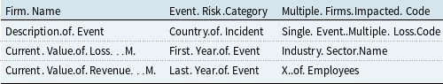
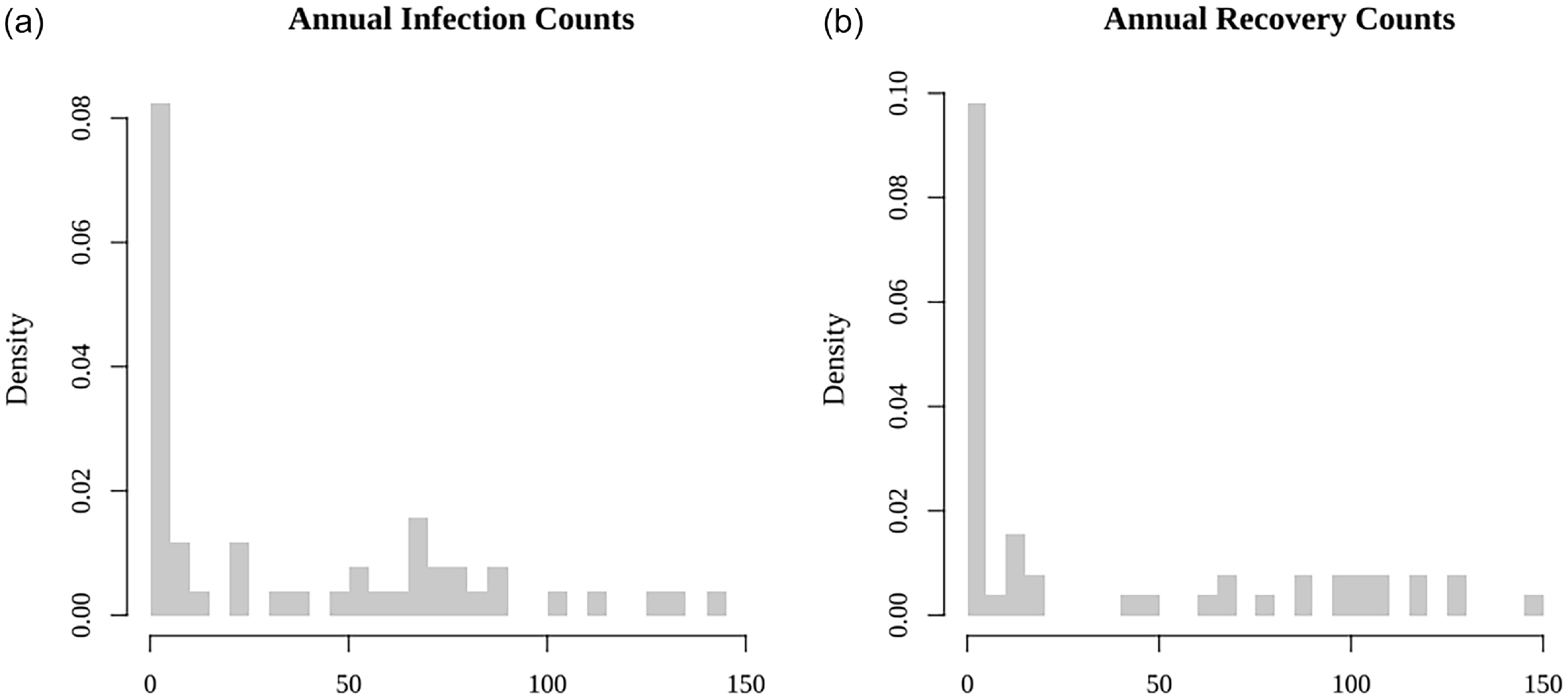

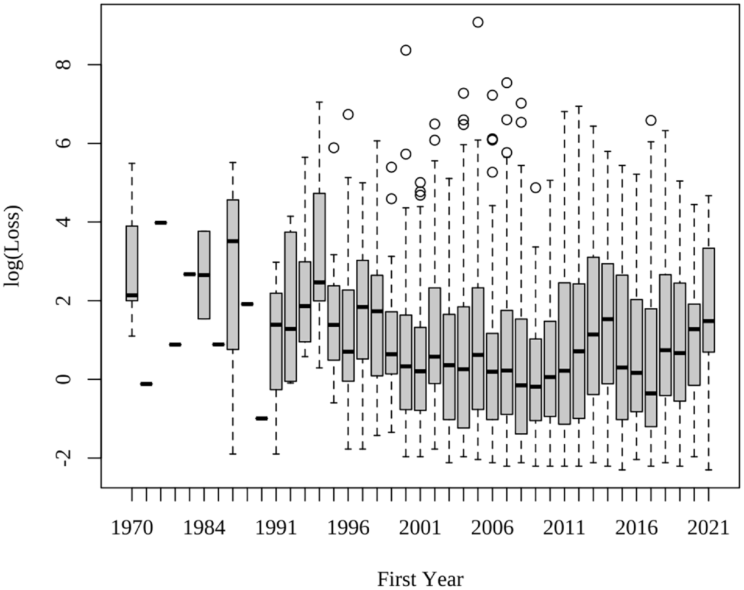
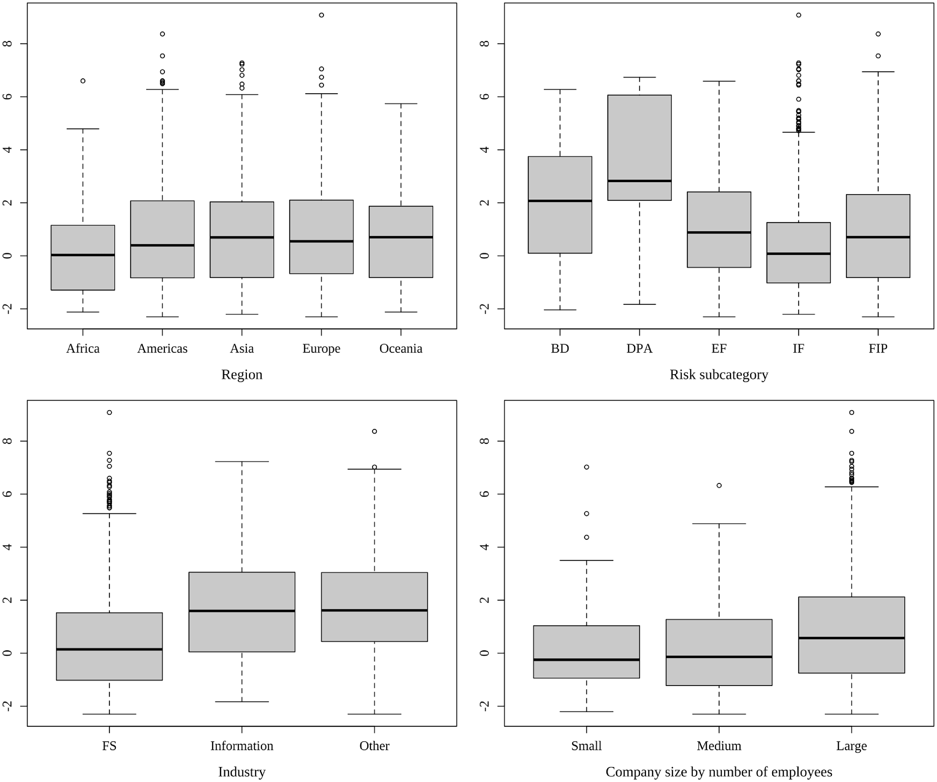
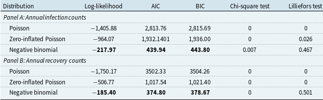

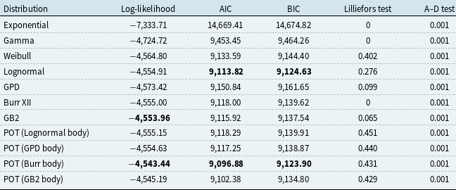

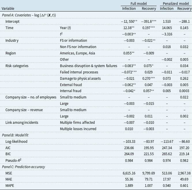


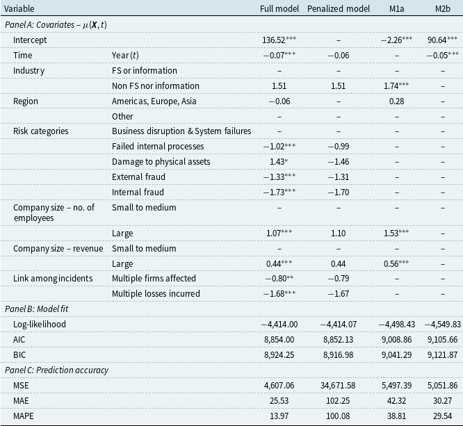

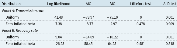


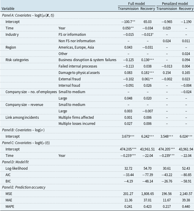


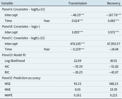


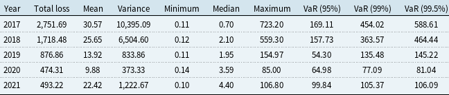
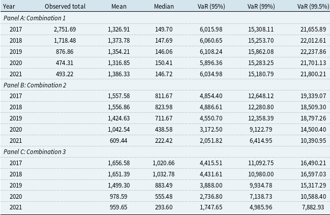

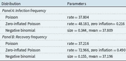
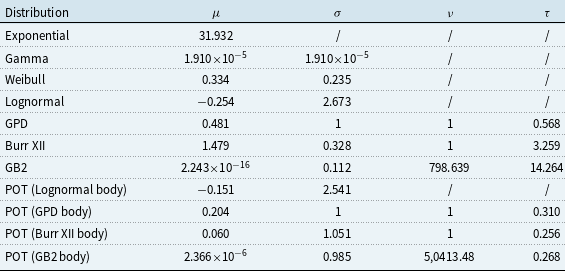
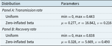
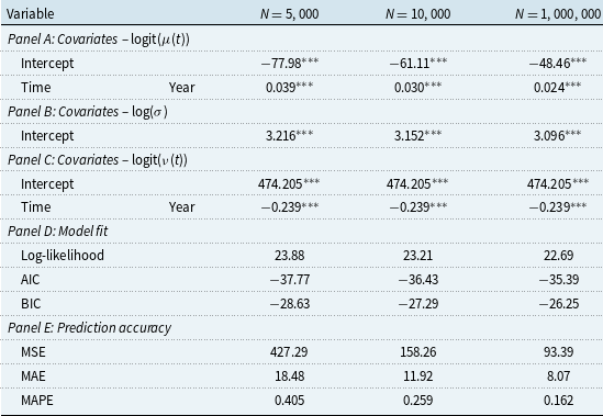


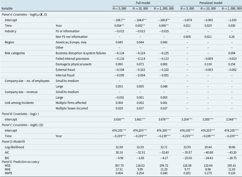


 Open access