


1. INTRODUCTION
This paper aims to measure the bed roughness of contemporary subglacial and deglaciated terrains at analogous length scales. We define bed roughness as the vertical variation of terrain over a given horizontal distance (Siegert and others, Reference Siegert, Taylor and Payne2005; Rippin and others, Reference Rippin, Vaughan and Corr2011). Accurate quantification of bed roughness beneath ice sheets is important because it is a primary control on basal drag and therefore ice flow velocity (Siegert and others, Reference Siegert, Taylor and Payne2005; Bingham and others, Reference Bingham2017). Subglacial obstacles of ~0.5–1 m in both amplitude and horizontal wavelength have been shown theoretically to exert critical basal drag (Weertman, Reference Weertman1957; Kamb, Reference Kamb1970; Nye, Reference Nye1970; Hubbard and Hubbard, Reference Hubbard and Hubbard1998; Hubbard and others, Reference Hubbard, Siegert and McCarroll2000; Schoof, Reference Schoof2002); however, these obstacle dimensions lie below the resolution achievable by radio-echo sounding (RES) across ice sheets. Several authors have nevertheless explored the relationship of higher amplitude (several 100 m) and longer wavelength (hundreds of m to several km) bed roughness and ice dynamics across ice sheets using available RES data. These analyses have suggested that beds beneath contemporary ice streams are relatively smooth, with roughness values decreasing downstream, whilst in surrounding areas of slower ice flow, the beds are relatively rougher (Siegert and others, Reference Siegert, Taylor, Payne and Hubbard2004; Rippin and others, Reference Rippin, Bamber, Siegert, Vaughan and Corr2006, Reference Rippin, Vaughan and Corr2011; Callens and others, Reference Callens2014). As a consequence, basal roughness is regarded as one of the controls on ice-stream location, in particular for ice streams not topographically controlled by deep valleys (Siegert and others, Reference Siegert, Taylor, Payne and Hubbard2004; Bingham and Siegert, Reference Bingham and Siegert2009; Winsborrow and others, Reference Winsborrow, Clark and Stokes2010; Rippin, Reference Rippin2013).
While a relationship between bed roughness and ice dynamics is intuitive, quantifying such a relationship has proved elusive and several studies have produced findings that should be explored further. For example, it has been observed that fast flowing ice can also occur over a rough, hard bed (Schroeder and others, Reference Schroeder, Blankenship, Young, Witus and Anderson2014). The reasons for a smooth bed underneath fast-flowing ice can be varied, for example the existence of fine-grained sediments vs. streamlined topography (Li and others, Reference Li2010; Rippin and others, Reference Rippin2014). Ice-stream beds can be smooth along ice flow (parallel) and rough across flow (orthogonal) (King and others, Reference King, Hindmarsh and Stokes2009; Bingham and others, Reference Bingham2017), showing that the direction of bed roughness measurements is extremely important. Palaeo-ice-stream beds show the same pattern (Gudlaugsson and others, Reference Gudlaugsson, Humbert, Winsborrow and Andreassen2013; Lindbäck and Pettersson, Reference Lindbäck and Pettersson2015). Geology can have a strong control on the roughness underneath fast-flowing ice as shown in previously glaciated gneiss terrains (Krabbendam and Bradwell, Reference Krabbendam and Bradwell2014). An increase in landform elongation ratios in a palaeo-ice stream has been related to the change from a rough to smooth bed (Bradwell and Stoker, Reference Bradwell and Stoker2015). The points raised by these studies demonstrate that bed roughness and its relationship to ice dynamics is complex. By using Digital Terrain Models (DTMs) from now-exposed palaeo-ice streams to calculate bed roughness, we propose that it may be possible to explore these complexities in more detail because the bed of a palaeo-ice stream can be directly observed over its entirety at much higher spatial resolutions than contemporary ice-stream beds.
The bed roughness of contemporary ice sheets has been calculated along 1-D topographic profiles (from RES tracks) predominantly using two different approaches, frequency domain methods for example Fast Fourier Transform (FFT) analysis (e.g. Taylor and others, Reference Taylor, Siegert, Payne and Hubbard2004; Siegert and others, Reference Siegert, Taylor and Payne2005; Bingham and Siegert, Reference Bingham and Siegert2007; Li and others, Reference Li2010; Rippin, Reference Rippin2013) and space domain methods for example Standard Deviation (SD) (Layberry and Bamber, Reference Layberry and Bamber2001; Rippin and others, Reference Rippin2014). Radar specularity has also been used to infer bed roughness (e.g. Schroeder and others, Reference Schroeder, Blankenship, Young, Witus and Anderson2014). The scale of bed roughness measurements has mostly been controlled by the spacing between flight tracks, and the along-track resolution, which is a function of the radar system used. Ice-sheet scale studies have typically used track spacing of several kilometres with an along track resolution of a few metres (Siegert and others, Reference Siegert, Taylor, Payne and Hubbard2004; Rippin and others, Reference Rippin, Bamber, Siegert, Vaughan and Corr2006; Bingham and others, Reference Bingham, Siegert, Young and Blankenship2007). Higher resolution radar imaging by King and others (Reference King, Hindmarsh and Stokes2009, Reference King, Pritchard and Smith2016) and Bingham and others (Reference Bingham2017) has shown topographic detail that cannot be captured by the larger scale studies, and is similar to the detail available on deglaciated terrains from DTMs and bathymetric data unconstrained by ice cover (e.g. Perkins and Brennand, Reference Perkins and Brennand2014; Bradwell and Stoker, Reference Bradwell and Stoker2015; Margold and others, Reference Margold, Stokes and Clark2015). Using DTMs also allows bed roughness to be measured in 2-D and at much smaller scales. The resolution of DTMs is becoming finer, with pixels down to a few metres or less (e.g. LiDAR; Salcher and others, Reference Salcher, Hinsch and Wagreich2010; Putkinen and others, Reference Putkinen2017). Analysis of DTMs from deglaciated areas provides an opportunity to show what is being missed when bed roughness measurements are interpolated across widely spaced RES transects. Bed roughness calculations made on this terrain can also be much more easily linked to the geomorphological and geological character of the bed because individual landforms and geological variation can be observed directly.
In this study, we compare the bed roughness of the deglaciated, Devensian, Minch Palaeo-Ice Stream (MPIS) and surrounding areas in NW Scotland, with the contemporary Institute and Möller Ice Streams (IMIS) in West Antarctica. The bed roughness of both ice streams is quantified along transects with the same grid spacing, but for the palaeo-ice stream is also calculated between transects. We test how several parameters influence the measurement and interpretation of bed roughness. Firstly, we gauge whether the method used to measure bed roughness, FFT analysis or SD, produces different results. Secondly, we explore whether RES track spacing is sufficient to capture bed roughness trends. Thirdly, we compare bed-roughness results from transects that have the same grid spacing as RES data with results calculated down to the DTM pixel resolution. Finally, we show how the orientation of transects in relation to ice flow direction influences bed-roughness results.
2. DATA AND METHODS
2.1. Study sites and data
The MPIS drained the NW sector of the British and Irish Ice Sheet during the Devensian (Weichselian) Glacial Period (116–11.5 ka BP) and has a well-documented glacial landform and sediment record (Bradwell and others, Reference Bradwell2008a; Bradwell and Stoker, Reference Bradwell and Stoker2015; Fig. 1). Its onset zone lies in the mountainous NW Highlands of mainland Scotland, with peaks up to ~1000 m above present-day sea level (m a.s.l.). At its maximum extent, several ice-stream tributaries flowed from breaches (at ~300 m a.s.l.) in the present-day watershed in the NW Highlands mainland out to the shelf edge, at ~200 m below present-day sea level (Bradwell and others, Reference Bradwell, Stoker and Larter2007, Reference Bradwell2016; Bradwell and Stoker, Reference Bradwell and Stoker2015; Krabbendam and others, Reference Krabbendam, Eyles, Putkinen, Bradwell and Arbelaez-Moreno2016). MPIS likely reached its maximum extent at ~26–28 ka (Chiverrell and Thomas, Reference Chiverrell and Thomas2010; Clark and others, Reference Clark, Hughes, Greenwood, Jordan and Sejrup2012; Praeg and others, Reference Praeg2015; Bradwell and others, Reference Bradwell, Stoker, Dowdeswell, Canals, Jakobsson, Todd, Dowdeswell and Hogan2016).
Study site locations. (a) The Minch Palaeo-Ice Stream (MPIS), in NW Scotland. MPIS flow paths, that is areas of fast-flowing ice, are from Bradwell and others, (2007). The flow path with white arrows is the Laxfjord tributary. The coarse grid (30 × 10 km) set up to mimic RES transects in (b), is shown in white. The fine grid (2 × 2 km) is over the Ullapool megagroove area and is shown in cyan. Inset map shows the location of the main image. (b) Institute and Möller Ice Streams (IMIS), in West Antarctica. RES transects are shown in black. The inset map shows the location of IMIS (blue box). Ice velocity from Rignot and others (Reference Rignot, Mouginot and Scheuchl2011) and Mouginot and others, (Reference Mouginot, Scheuchl and Rignot2012).

IMIS drain the West Antarctic Ice Sheet into Ronne Ice Shelf (Fig. 1). Ice surface velocities are up to 400 m a−¹ (Rignot and others, Reference Rignot, Mouginot and Scheuchl2011). The inferred occurrence of sediments at the bed of Institute Ice Stream has been interpreted to be associated with a smooth bed (Bingham and Siegert, Reference Bingham and Siegert2007; Siegert and others, Reference Siegert2016). The Ellsworth Trough Tributary, a tributary of Institute Ice Stream, is topographically controlled (Ross and others, Reference Ross2012).
We compare MPIS with IMIS due to their relatively comparable scale. IMIS ice thickness varies between ~50 and 3000 m (Fretwell and others, Reference Fretwell2013). A maximum ice thickness of 750–1000 m has been modelled for MPIS (Hubbard and others, Reference Hubbard2009; Kuchar and others, Reference Kuchar2012). IMIS drain an area of 140 000 km2 and 66 000 km2, respectively (Bingham and Siegert, Reference Bingham and Siegert2009), While MPIS drained an area of 15 000–20 000 km2 (Bradwell and others, Reference Bradwell, Stoker and Larter2007; Bradwell and Stoker, Reference Bradwell and Stoker2015). Institute Ice Stream is up to 82 km wide and the fast flowing section of the main trunk is 100 km long (Scambos and others, Reference Scambos, Bohlander, Raup and Haran2004). MPIS was 40–50 km wide and 200 km long in total (Bradwell and Stoker, Reference Bradwell and Stoker2015). MPIS had a discharge flux of 12–20 Gt a−1 (Bradwell and Stoker, Reference Bradwell and Stoker2015) compared with 21.6 and 6.4 Gt a−1 for IMIS, respectively (Joughin and Bamber, Reference Joughin and Bamber2005).
For contemporary ice streams in Antarctica, the data used were RES transects with an along track resolution of 10 m, and a grid spacing of 30 × 10 km (Rippin and others, Reference Rippin2014). Data were acquired in the 2010/11 austral summer using the Polarimetric Airborne Survey Instrument (PASIN) with a frequency of 150 MHz (Ross and others, Reference Ross2012). PASIN has retrieved bed-echoes through 4200 m thick ice (Vaughan and others, Reference Vaughan2006). Crossover analysis gave RMS differences of 18.29 m for ice thickness (Ross and others, Reference Ross2012). The location of the data was determined using a differential GPS with a horizontal accuracy of ~5 cm. The reflections returned from the ice-stream bed were processed semi-automatically. The ice thickness (calculated every ~10 m) was subtracted from ice surface elevations to calculate the bed elevations (Ross and others, Reference Ross2014). For more detail on acquisition and processing of the RES data see Rippin and others (Reference Rippin2014) and Ross and others (Reference Ross2012, Reference Ross2014). This dataset was used by Rippin and others (Reference Rippin2014) to calculate bed roughness using both FFT analysis and SD.
Two high-resolution datasets were used to calculate bed roughness of the MPIS. For the onshore area, the NEXTMap DTM with a 5 m horizontal resolution and a 1 m vertical resolution, was used (Bradwell, Reference Bradwell2013). NEXTMap DTM tiles were downloaded from the Centre for Environmental Data Analysis (CEDA) Archive (Intermap Technologies, 2009). For the offshore area, Bathymetric Multi-Beam Echosounder Survey data (MBES) were used. The MBES data subset has a resolution of 4 m and encompasses the Little Minch and the southern area of The Minch (Fig. 1). The surveys around NW Scotland were undertaken by the Maritime & Coastguard Agency (MCA) between 2006 and 2012. For more detail on acquisition and processing of MBES data see Bradwell and Stoker (Reference Bradwell and Stoker2015) or the Reports of Survey, which can be requested from MCA, the UK Hydrographic Office, the British Geological Survey or the Natural Environment Research Council. MPIS is characterised by numerous elongate landforms that show a higher elongation ratio than those in adjacent areas (Bradwell and others, Reference Bradwell, Stoker and Krabbendam2008b). Onshore, the bed of the palaeo-ice stream is dominated by bedrock (i.e. hard-bed) landforms (Krabbendam and Bradwell, Reference Krabbendam, Bradwell, Lukas and Bradwell2010; Clark and others, Reference Clark2018) including bedrock megagrooves, crag and tails, whalebacks and roches moutonnées (partly within a cnoc-and-lochan landscape, especially characteristic of Scotland's northwest region, Assynt), with few soft-sediment covered landforms (e.g. Bradwell and others, Reference Bradwell, Stoker and Larter2007; Bradwell, and others, Reference Bradwell, Stoker and Krabbendam2008b; Krabbendam and Bradwell, Reference Krabbendam and Bradwell2011; Bradwell, Reference Bradwell2013). In the Minch and further offshore on the Hebrides Shelf, the bed of the palaeo-ice stream comprises more soft-sediment landforms, such as drumlinoid features, although streamlined bedrock, crag-and-tail features and megagrooves are also present, particularly in the inner Minch (Bradwell and Stoker, Reference Bradwell and Stoker2015, Reference Bradwell, Stoker, Dowdeswell, Canals, Jakobsson, Todd, Dowdeswell and Hogan2016; Ballantyne and Small, Reference Ballantyne and Small2018). Overdeepened basins occur, in particular, close to the present-day coast, which is in part characterised by a fjord system (Bradwell and Stoker, Reference Bradwell, Stoker, Dowdeswell, Canals, Jakobsson, Todd, Dowdeswell and Hogan2016; Bradwell and others, Reference Bradwell, Stoker, Dowdeswell, Canals, Jakobsson, Todd, Dowdeswell and Hogan2016). Increases in ice velocity are inferred from changes to landform elongation ratios located on the central Minch inner shelf (East Shiant Bank), which Bradwell and Stoker (Reference Bradwell and Stoker2015) suggested is caused by the bed substrate changing from rough bedrock to smooth sediment.
2.2. Methods
Bed roughness along RES tracks in the Antarctic ice sheet and Greenland ice sheet has predominantly been quantified using either FFT analysis (e.g. Bingham and Siegert, Reference Bingham and Siegert2009; Rippin, Reference Rippin2013; Rippin and others, Reference Rippin2014), or SD of bed elevations (e.g. Layberry and Bamber, Reference Layberry and Bamber2001; Rippin and others, Reference Rippin2014). FFT analysis transforms bed elevations into wavelength spectra (Gudlaugsson and others, Reference Gudlaugsson, Humbert, Winsborrow and Andreassen2013), producing a power spectrum (Bingham and Siegert, Reference Bingham and Siegert2009), which is a measure of the intensity (power) of different wavelength obstacles along a transect. SD is a measure of variation in amplitude. Applied to elevation data, a higher SD implies a greater spread between the high and low elevations, and thus a rougher bed. Both methods were used on MPIS and IMIS datasets to provide a comparison.
Both roughness methods were applied to a 2-D dataset from a deglaciated terrain, MPIS, and were compared with a 1-D dataset from a glaciated terrain, IMIS. We constructed an ‘artificial’ grid of transects spaced 30 × 10 km apart over the high-resolution NEXTMap DTM and MBES bathymetry of the deglaciated MPIS to mimic a gridded RES survey over the glaciated IMIS (Fig. 1). The transect spacing replicates the spacing and resolution of RES transects used by Rippin and others (Reference Rippin2014) on IMIS. Points were constructed every 10 m along all transects, and the x, y and z coordinates were extracted from NEXTMap DTM and MBES bathymetry.
Before bed roughness can be calculated using SD or FFT analysis, the elevation data have to be detrended to remove large wavelengths caused by mountains and valleys, which would otherwise dominate roughness measurements (Shepard and others, Reference Shepard2001; Smith, Reference Smith2014). We are interested in roughness obstacles at a smaller scale than this, that is those which affect drag. The elevation data for each transect were detrended in R using the difference function (where difference = 2). This detrending method does not require a moving window, which removes one of many variables that affect the final bed-roughness results (Prescott, Reference Prescott2013; Smith, Reference Smith2014). SD was then calculated along transects using a moving window size of 320 m (32 points) following previous studies (e.g. Taylor and others, Reference Taylor, Siegert, Payne and Hubbard2004; Li and others, Reference Li2010). Where transects crossed lakes and coast, bed roughness values were removed to prevent bias towards smooth surfaces (Gudlaugsson and others, Reference Gudlaugsson, Humbert, Winsborrow and Andreassen2013) using the Ordnance Survey Meridian 2 lake regions shapefile (Ordnance Survey, 2017). FFT analysis requires continuous along-track data. For gaps of >100 m long (10 points), the transects were ‘cut’ (Rippin and others, Reference Rippin2014). Note that, in the onshore DTM analysis, a lake functions like a data gap. FFT analysis was not calculated across these gaps. Following previous studies (e.g. Taylor and others, Reference Taylor, Siegert, Payne and Hubbard2004; Bingham and Siegert, Reference Bingham and Siegert2009; Rippin and others, Reference Rippin2014), FFT analysis was calculated along transects using a window of 2N points, where N = 5 giving a window length of 320 m (32 points). The total roughness parameter was then defined by calculating the integral of the power spectra for every window. Roughness at all scales up to the length of the window was integrated.
The bed-roughness calculations from both methods were then interpolated using the Topo to Raster tool in ArcMap, with a 1 km output cell size. The interpolated values were smoothed with a 10 km radius circle and a buffer of 2.5 km was applied either side of the transects. This allowed us to replicate the type of processed results that would be extracted from a RES survey. The same method as described above was applied to the RES transects for IMIS. The difference in bed roughness values was calculated for MPIS and IMIS at locations where transects crossed. Most SD results presented here are not normalised, but shown as absolute values in metres. However, when presented alongside the FFT results, the SD results were normalised, to enable a comparison. Following the post-processing stages of interpolation, buffering and smoothing, the data were normalised using a linear transformation. The results from both sites and both methods were re-scaled so that values range between 0 and 1.
A grid of transects spaced 2 × 2 km apart was also created for the Ullapool megagroove area (Fig. 1), a well-characterised part of the onset zone of MPIS (Bradwell and others, Reference Bradwell, Stoker and Krabbendam2008b). This finer grid was used to measure roughness in between the gaps created when widely spaced RES grids are used underneath contemporary ice sheets. A 2 × 2 km grid allowed interpolation between transects and was aligned approximately parallel and orthogonal to palaeo-ice flow. Roughness was calculated using the same method as the larger grid, but the interpolation resolution was 200 m, and the values were smoothed using a 2 km radius circle. Roughness was also calculated for transects parallel and orthogonal to palaeo-ice flow, allowing differences in bed roughness between palaeo-ice flow directions to be calculated. Within the area of the 2 × 2 km grid, Bradwell and others (Reference Bradwell, Stoker and Krabbendam2008b) identified a bedform continuum, which equates to an erosional transition. This transition was interpreted as a thermal boundary by Bradwell and others (Reference Bradwell, Stoker and Krabbendam2008b), and bed roughness values from the inferred areas of warm and cold bed conditions were extracted from the smoothed interpolation, to quantify differences in roughness between these areas.
Finally, bed roughness was calculated over the entire onshore study area of the MPIS using a 2-D approach. The 2-D approach uses SD to calculate bed roughness across surfaces, rather than along 1-D transects. The 2-D method allows the full coverage and resolution of the NEXTMap data to be analysed, so that bed roughness can be calculated for the gaps in between 1-D transects. For every pixel, a circular window with a 320 m diameter was used for detrending and calculating bed roughness to match the results from the 1-D approach. The NEXTMap DTM was detrended by subtracting a smoothed bed from the original terrain. SD was calculated from the detrended raster for each 320 m circular window. We present both unsmoothed and smoothed 2-D data, to enable comparison with the smoothed 1-D results. Unsmoothed 2-D data allow us to look at the roughness calculations in more detail, whereas smoothed data show broader trends. Bed roughness was also calculated using the same approach above (except with a smaller 100 m window size) for all north-south pixels and all east-west pixels to assess directionality.
3. RESULTS
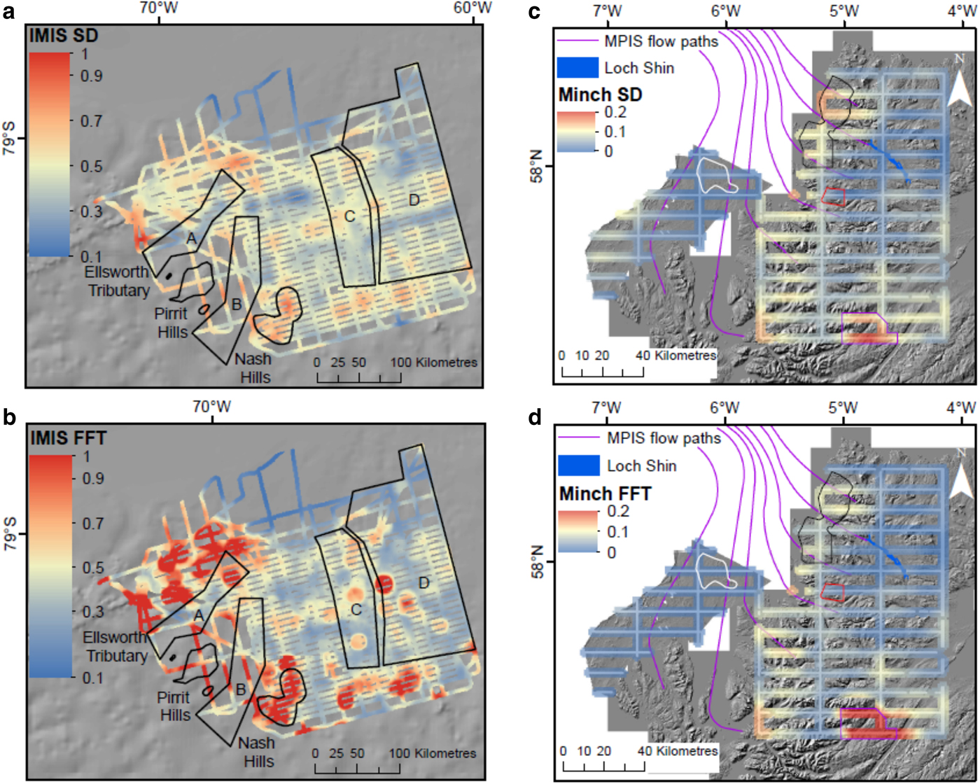
The 1-D roughness results calculated using SD for IMIS (Fig. 2c) are, as expected, similar to those found by Rippin and others (Reference Rippin2014) using FFT analysis (Fig. 2b). The locations of high and low values are similar but the relative magnitude of roughness trends appears reduced for SD (Fig. 2). Table 1 shows a slightly smaller range in roughness values for IMIS SD and similar means for both methods. It should be noted that SD roughness results are reported in the text as real values but are normalised in Figure 2 and Table 1 to enable comparison with FFT analysis. IMIS SD roughness values vary between ~0.5 and 4 m. Lower roughness values of 0.5–1 m are generally located underneath the ice-stream tributaries, whereas higher roughness values (2.5–3.8 m) are associated with the Pirrit Hills and Nash Hills in the intertributary areas. The Ellsworth Tributary, a tributary of Institute Ice Stream, has low bed roughness values except where it joins the main trunk (~2.7 m). Similarly, Area D, a tributary of Möller Ice Stream, has mostly low roughness values, but with some higher bed roughness values (up to 2.8 m). Areas B and C, tributaries of Institute Ice Stream, generally have rougher beds than Areas A and D (up to 3.4 m). Parts of the inter-tributary area, however, have low roughness values (1 m). Thus, although there is a broad correlation between roughness and ice velocity, there are significant exceptions.
Bed roughness calculated for MPIS and IMIS using SD and FFT analysis (window size = 320 m). SD and FFT data are normalised. MPIS flow paths after Bradwell and others (Reference Bradwell, Stoker and Larter2007). For MPIS; the Ullapool megagrooves are outlined in red, the cnoc-and-lochan landscape (including Assynt) to the north is outlined in black, the exposed bedrock (East Shiant Bank) in the Minch is outlined in white, and the Aird is outlined in purple. For IMIS, Institute Ice Stream tributaries are labelled A, B and C, whilst the Möller Ice Stream tributary is labelled D. (a) MPIS roughness derived from SD (m). (b) MPIS roughness derived from FFT analysis (total roughness parameter). (c) IMIS roughness derived from SD (m). (d) IMIS roughness derived from FFT analysis (total roughness parameter).
Statistics of bed roughness results for MPIS and IMIS, using both methods

These are normalised values. The maximum value and minimum value across all datasets was used to normalize.
The SD bed roughness values for MPIS have a lower range (0–1 m) compared with IMIS (0.5–4 m). This also applies to the normalised SD values. The FFT bed roughness values for MPIS also have a lower range compared to IMIS (Table 1). The SD bed roughness values are lower (0.1–0.5 m) in the trunk of MPIS compared with the onset zones onshore (Fig. 2c). Most of the bed in the Minch is sediment covered, but some bedrock has been mapped (Fyfe and others, Reference Fyfe, Long and Evans1993; Bradwell and Stoker, Reference Bradwell and Stoker2015), which is slightly rougher (0.2 m) than the sediment dominated areas (0.1 m). The bedrock in the Minch is significantly smoother than the onshore bedrock of the cnoc-and-lochan landscape (Fig. 2c, d) in the onset zone (by up to 0.7 m). The 30 × 10 km grid is too low in resolution to give a detailed analysis of the transition between rough bedrock and smooth sediment in the Minch (Fig. 2). Within the Minch (bathymetry data), the flowlines coincide with smooth values (~0.1 m) (Fig. 2). This pattern contrasts with most of the flowlines in MPIS onset zones (Fig. 2), where values are rougher (0.2–0.9 m). This compares to higher bed roughness values from IMIS, which vary from 1 to 2.9 m and 1–3.8 m in the tributary and intertributary areas, respectively (Fig. 2). The highest roughness values on the mainland of NW Scotland are found in the southern area (the Aird) of the 30 × 10 km grid (1 m) (Fig. 2), whilst the lowest values are concentrated in the centre and east (0.2 m) (Fig. 2). The bed roughness results from SD and FFT analysis show similar trends in high and low values for MPIS (Fig. 2c, d). For example, over the Ullapool megagrooves, both methods produce bed roughness values of 0.1 (normalised values). However, the results calculated using SD are higher overall than those calculated from FFT analysis (higher mean in Table 1). This difference is largest over the cnoc-and-lochan area, where the SD results are up to 3.5 times higher. SD bed roughness results show slightly more variation than those calculated from FFT (Fig. 2c, d). For example, bed roughness values from the top east-west transect (Fig. 2c, d) are 0.01 when calculated using FFT analysis, but vary between 0.06 and 0.1 when calculated using SD.The bed roughness trends from the 30 × 10 km grid (Fig. 3c) match those calculated from the smoothed 2-D approach (Fig. 3b) relatively well, particularly, the high roughness values over the cnoc-and-lochan landscape (3 m compared with 1 m), and low roughness values over the central and NE areas. The unsmoothed 2-D results (Fig. 3a) give a much more detailed picture of bed roughness. Within the cnoc-and-lochan terrain there are significant local variations in roughness that are not apparent in the smoothed 2-D data (Fig. 3a, b), While the bedrock of the East Shiant Bank is visible in the unsmoothed roughness data but not the smoothed (Fig. 3a, b).
Bed roughness calculated using SD for all NEXTMap DTM pixels using a moving window of 320 m (2-D). Values are not normalised. The exposed bedrock (East Shiant Bank) in the Minch is outlined in white. The Ullapool megagrooves are outlined in red. The cnoc-and-lochan landscape (including the Assynt) to the north is outlined in black. The Aird is outlined in purple. (a) Bed roughness of MPIS onset zone with flow paths after Bradwell and others (Reference Bradwell, Stoker and Larter2007). Blue boxes are inselbergs and mountain massifs that are missed by the 1-D 30 × 10 km transects. These include Ben Mor Coigach massif, Ben Stack, the Assynt massif, the Fannichs, and Liathach. Red boxes show Loch Ewe and Little Loch Broom, which appear rough on the 1-D grid but smooth using the 2-D data. (b) Bed roughness from (a) that has been resampled to 1 km resolution and smoothed using the same window size as that used for the bed roughness measurements calculated using the 30 × 10 km grid. (c) Bed roughness from the 1-D 30 × 10 km.

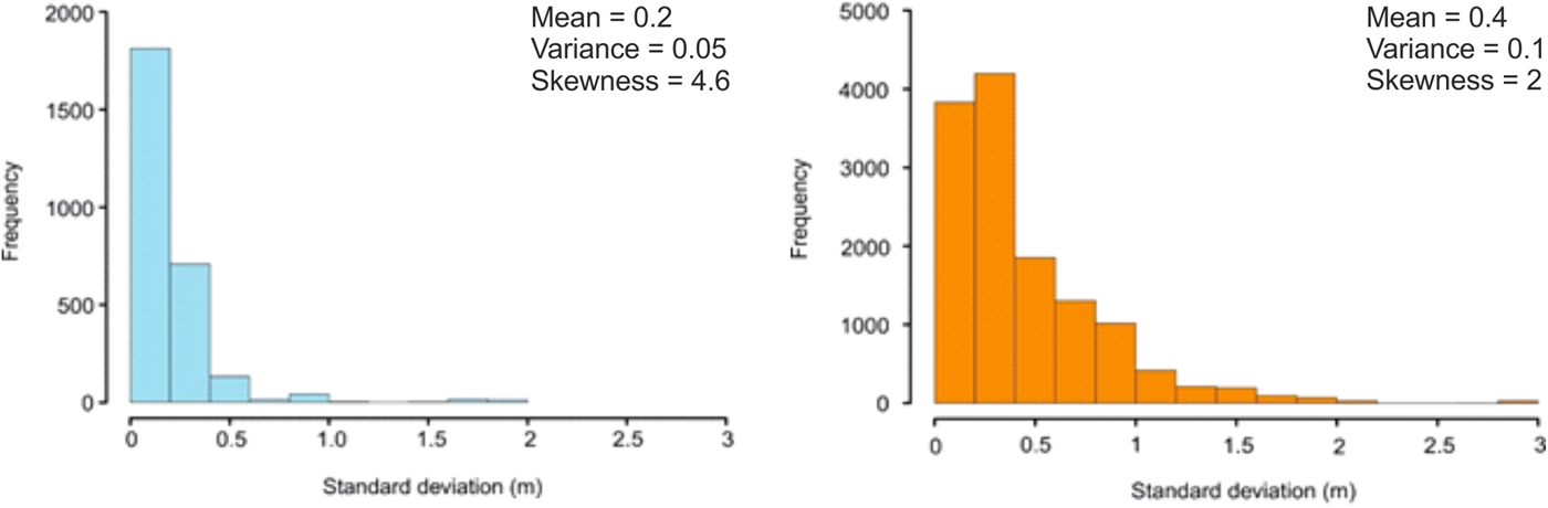
The 2 × 2 km grid records higher roughness over the Ullapool megagrooves compared with the larger grid (0.3 m compared with 0.7 m) (Figs 2 and 4 respectively). The distribution of bed roughness values between the areas interpreted by Bradwell and others (Reference Bradwell, Stoker and Krabbendam2008b) as cold and warm bed conditions (Fig. 4a) over the Ullapool megagrooves show a clear difference. The area with a cold bed has predominantly lower bed roughness values, with a mean of 0.2 m, compared with the area where the bed was warm, with a mean of 0.4 m (Fig. 5). There is a clear transition to higher bed roughness values over the megagrooves compared with the surrounding areas (Fig. 4a).
Roughness measured along transects (white lines, grid spacing of 2 × 2 km) over the Ullapool megagrooves (see Fig. 1 for location). The transects are approximately parallel and orthogonal to palaeo-ice flow (Solid black lines with arrows, east to west). 1 is an area of no glacial streaming (cold-based ice), 2 is an area of subtle streamlined landforms between the dotted and dashed lines (warm-based ice). Between the dotted lines, 3 is an area of strong glacial streamlining (warm-based ice). Palaeo-flow direction and areas of glacial streaming after Bradwell and others (Reference Bradwell, Stoker and Krabbendam2008b). Values are not normalised. (a) Roughness calculated along all transects. (b) Roughness calculated along transects parallel to flow. (c) Roughness calculated along transects orthogonal to flow. (d) The magnitude difference between (b) and (c).

Bed roughness distributions in cold-based (blue) and warm-based (orange) areas from the 2 × 2 km grid over the Ullapool megagrooves. Cold-based and warm-based areas are defined by Bradwell and others (Reference Bradwell, Stoker and Krabbendam2008b). Values are not normalised.
4. DISCUSSION
Our results show that similar patterns of bed roughness are found in both contemporary and palaeo-ice stream settings, using the same transect spacing and along-transect resolution (Fig. 2). High and low roughness values can generally be found in areas of fast ice flow. This suggests that bed roughness is not always a controlling factor on the location of ice streaming. Overall, the bed roughness results for IMIS are higher than MPIS. One reason for this difference could be the vertical resolution of RES data, which is lower compared with DTM data (5 m vs. 1 m, respectively). Postglacial sedimentation could be one of the causes of this. For example, a thin layer (0.1–10 m) of postglacial sediment deposition occurs in the Minch (Fyfe and others, Reference Fyfe, Long and Evans1993; Bradwell and Stoker, Reference Bradwell and Stoker2015), which will reduce the amplitude of small-scale glacial features. Yet this is unlikely to be the case onshore, where predominantly exposed bedrock with more localised areas of postglacial sediment prevails (Krabbendam and Bradwell, Reference Krabbendam, Bradwell, Lukas and Bradwell2010). Conversely, topographic profiles collected using RES are an average of the radar trace (King and others, Reference King, Pritchard and Smith2016), which could cause such data to be slightly smoothed in comparison with data from visible surfaces for example DTMs. Without being able to see the entire bed of IMIS it is difficult to provide a definitive answer. We suggest that the reason for higher bed roughness in IMIS could be due to the difference in elevation range between the two locations. MPIS has an elevation range of 1493 m, While IMIS has an elevation range of 3582 m (Fretwell and others, Reference Fretwell2013).
4.1. SD vs. FFT analysis methods
Our comparison between SD and FFT analysis at the 1-D scale for MPIS and IMIS showed similar broad trends of bed roughness, but there were differences (Fig. 2). For MPIS, the cnoc-and-lochan landscape appears rougher in the SD than in FFT (Fig. 2). Cnoc-and-lochan landscapes typically contain abundant lakes, which appear on a DTM as a flat surface. These are removed from the dataset to avoid bias towards a smooth surface. For FFT analysis to be carried out, transects measuring <320 m between lakes are also removed from the data, causing data gaps. Where there are multiple lakes along a transect with <320 m between them, the SD method measures a high roughness value. FFT analysis cannot capture this variation in terrain. Some transects that are not impacted by lakes also have higher bed roughness values calculated from SD compared with FFT analysis. Both methods essentially measure the amplitude of the bed obstacles (Rippin and others, Reference Rippin2014), but FFT analysis measures the frequency of vertical undulations (Bingham and Siegert, Reference Bingham and Siegert2009). We suggest that the FFT analysis is measuring similar frequencies of elevation change. The results from the SD method for the same landscape are rougher than FFT analysis, because it is measuring large amplitude changes between the numerous hills and lakes. Furthermore, FFT analysis (total roughness parameter) integrates roughness at all scales up to the window size, whereas SD is calculated for the window size only. This will cause higher roughness results measured using SD because the values are calculated over a larger horizontal length-scale (Shepard and others, Reference Shepard2001). Both methods have advantages and disadvantages in their application. FFT analysis emphasises roughness frequency whilst SD provides a more intuitive measure of roughness scales.
4.2. Transect spacing vs. complete coverage: what is missed?
Measuring bed roughness on a palaeo-ice stream allows us to assess the validity of RES transect spacing used to measure bed roughness on contemporary ice streams. The 30 × 10 km grid misses key areas of glacial landforms used to interpret MPIS ice dynamics, such as the transition from rough bedrock to smooth sediments in the bathymetry data (Fig. 2) (Bradwell and Stoker, Reference Bradwell and Stoker2015). For the onshore data, shifting the 30 × 10 km grid by a few km north or south would miss the Ullapool megagrooves altogether (Fig. 2). Entire inselbergs and mountain massifs are missed (blue boxes on Fig. 3): in the 2-D roughness maps these areas appear as very rough and it is known these had a profound effect on local ice dynamics (Bradwell, Reference Bradwell2005, Reference Bradwell2013; Finlayson and others, Reference Finlayson, Golledge, Bradwell and Fabel2011). Conversely, some areas appear rough on the 1-D transect but appear on the 2-D maps as fairly smooth (red boxes on Fig. 3). A much more detailed picture of 2-D bed roughness trends can be achieved without the smoothing employed by previous studies (Fig. 3a) (e.g. Rippin and others, Reference Rippin2014). For example, all the cnoc-and-lochan area appears rough on the smoothed 2-D data, but the unsmoothed data show that some parts are smooth (Fig. 3a, b). The 2-D method surpasses the detail that can be captured by the 1-D transects but does not allow for analysis of the bed roughness directionality (anisotropy). It is clear that exploring palaeo-ice-stream roughness is possible at much higher resolutions than for contemporary ice streams, and important insights regarding the roughness of subglacial terrain may thus be learnt from these environments (Gudlaugsson and others, Reference Gudlaugsson, Humbert, Winsborrow and Andreassen2013).
A 30 × 10 km grid is too widely spaced to capture bed roughness of some landform assemblages. The question of what grid size should be used is an important one. The Ullapool megagrooves for example, cover an area of 6 × 10 km and individual grooves are up to 4 km long (Krabbendam and others, Reference Krabbendam, Eyles, Putkinen, Bradwell and Arbelaez-Moreno2016). A grid size of 2 × 2 km is arguably more suitable (Fig. 4). The size of glacial landforms that can be measured at DTM resolution varies largely, ~10–105 m (Clark, Reference Clark1993; Bennett and Glasser, Reference Bennett and Glasser2009) and a grid size that can measure mega-groove bed roughness might not be appropriate for other landform assemblages. The landscape underneath ice streams has been captured in detail using RES grids with transects spaced 500 m apart (King and others, Reference King, Hindmarsh and Stokes2009, Reference King, Pritchard and Smith2016; Bingham and others, Reference Bingham2017). Importantly, these studies only used orthogonal transects because RES can pick up multiple landform crests parallel to ice flow (King and others, Reference King, Pritchard and Smith2016). Acquiring RES tracks at 500 m spacing for large areas is very challenging, but future surveys could be focused on locations where rough, streamlined topography is thought to be present (Bingham and others, Reference Bingham2017), or areas that could cause a future sea level rise through rapid retreat for example Thwaites Glacier (Joughin and others, Reference Joughin, Smith and Medley2014; DeConto and Pollard, Reference DeConto and Pollard2016). Drones or Unmanned Aerial Vehicles have the potential to make RES data collection with small track spacing more viable over large areas (e.g. Leuschen and others, Reference Leuschen2014).
4.3. The importance of transect orientation
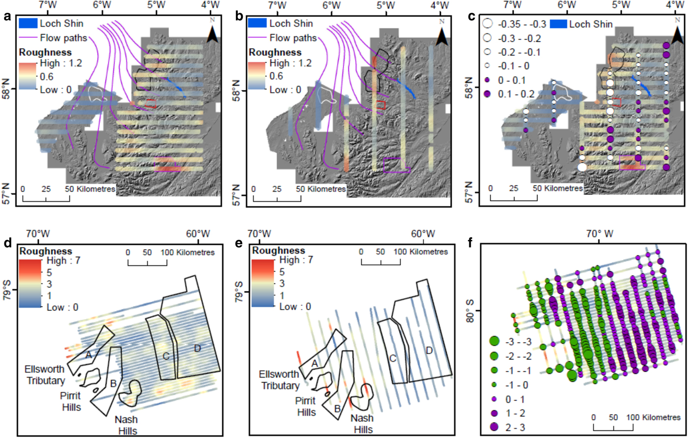
The locations of high roughness values over MPIS, measured by both SD and FFT analysis along transects, do not always reflect qualitative roughness seen in the DTM and bathymetry data. This problem has been investigated previously for bed roughness (e.g. Gudlaugsson and others, Reference Gudlaugsson, Humbert, Winsborrow and Andreassen2013; Rippin and others, Reference Rippin2014) and englacial layers (e.g. Ng and Conway, Reference Ng and Conway2004; Bingham and others, Reference Bingham2015), and transect orientation was shown to be important. To explore the influence of transect orientation on bed roughness we calculated bed roughness separately for north-south and east-west transects for both MPIS and IMIS (Fig. 6). Where transects cross each other, the difference in roughness was calculated (Fig. 6c, f). This was also done for transects on a pixel scale spacing for MPIS (Fig. 7). The difference in roughness of cross-cutting transects can be seen as a measure of directionality (anisotropy).
The relationship between bed roughness measurements and transect orientation for MPIS and IMIS. All bed roughness measurements were calculated using SD and values are not normalised. For MPIS: The exposed bedrock (East Shiant Bank) in the Minch is outlined in white. The Ullapool megagrooves are outlined in red. The cnoc-and-lochan landscape (including the Assynt) to the north is outlined in black. The Aird is outlined in purple. (a) Bed roughness for east-west MPIS transects. (b) Bed roughness for north-south MPIS transects. (c) The proportional circles show the east-west transects minus the north-south for MPIS. (d) Bed roughness for east-west IMIS transects. (e) Bed roughness for north-south IMIS transects. (f) The proportional circles show the east-west transects minus the north-south transects for IMIS.
The relationship between bed roughness measurements and transect direction for MPIS on a pixel scale. All bed roughness measurements were calculated using SD (window size = 100 m) and values are not normalised. The same interpolation and smoothing done for Figure 4 was used here. The exposed bedrock (East Shiant Bank) in the Minch is outlined in white. The Ullapool megagrooves are outlined in red. The cnoc-and-lochan landscape (including Assynt) to the north is outlined in black. The Aird is outlined in purple. (a) Bed roughness values calculated for each row of the DTM (east-west). (b) Bed roughness values calculated for each column of the DTM (north-south). (c) Plot of east-west minus north-south bed roughness.
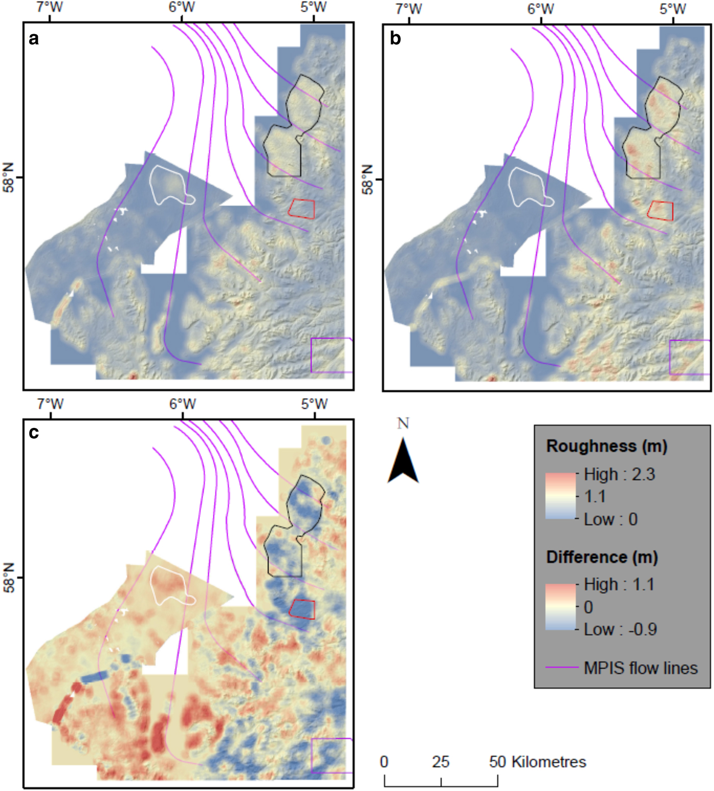
In MPIS some areas show a difference between east-west and north-south transects, suggesting significant anisotropy. The north-south transect along the West coast has higher roughness values (Fig. 6), notably for the lower part of the cnoc-and-lochan landscape on the exposed gneiss bedrock in the Assynt area (Krabbendam and Bradwell, Reference Krabbendam and Bradwell2014) and the edge of Ullapool mega grooves area (Bradwell and others, Reference Bradwell, Stoker and Krabbendam2008b). This same pattern is also apparent in more detail at the pixel scale (Fig. 7). In the Minch, the east-west pixels are rougher over the exposed bedrock (East Shiant Bank) (Fig. 7c), which is not shown in Figure 6 because of the wide transect spacing. In both cases, the rougher transects are orthogonal to palaeo-ice flow and support previous observations of bedrock smoothing by streaming ice (Bradwell and Stoker, Reference Bradwell and Stoker2015; Ballantyne and Small, Reference Ballantyne and Small2018). The east-west transects crossing the Aird are rougher than the north-south transects (Fig. 6). Closer inspection of the NEXTMap DTM reveals these rough values are located where the east-west transects cross deeply incised river valleys. Post-glacial erosion or sediment deposition can impact on palaeo-ice-stream bed roughness values. In IMIS east-west transects have higher roughness values predominantly in the tributaries labelled C and D, whilst the north-south transects have higher roughness values under tributaries A and B (Fig. 6). Although the direction of these transects is not related to ice flow as analysed by Rippin and others, (Reference Rippin2014), it shows that the direction of transects influences the bed roughness results for both contemporary and palaeo-ice streams.
For contemporary ice streams it has been shown that the transect orientation in relation to ice flow can bias interpretation (e.g. Rippin and others, Reference Rippin2014; Bingham and others, Reference Bingham2015; Bingham and others, Reference Bingham2017). Parallel to ice flow, the data tend to show smooth beds (Lindbäck and Pettersson, Reference Lindbäck and Pettersson2015) and undisrupted ice layering (Bingham and others, Reference Bingham2015), whereas data orthogonal to ice flow can show rough topography (Rippin and others, Reference Rippin2014; Bingham and others, Reference Bingham2017), which can be caused by streamlined features, for example mega grooves or mega-scale glacial lineations. These landforms have strong anisotropy (Spagnolo and others, Reference Spagnolo2017). The advantage of looking at palaeo-ice-stream beds compared with contemporary ice-stream beds is that the landforms can be observed directly. The strong anisotropy of the Ullapool megagrooves, already known from traditional geomorphological studies (Bradwell and others, Reference Bradwell, Stoker and Larter2007; Krabbendam and others, Reference Krabbendam, Eyles, Putkinen, Bradwell and Arbelaez-Moreno2016), is well captured by the 2 × 2 km grid results (Fig. 4b, c, d). Flow parallel transects are smoother (0.4 m), than the orthogonal transects (1 m). The roughness orthogonal to palaeo-ice flow is up to 2× higher than parallel palaeo-ice flow. The same pattern is shown in Figure 7. The formation of hard-bed megagrooves smooths the bed along ice flow but may lead to increased roughness orthogonal to ice flow, for instance by lateral plucking (Krabbendam and Bradwell, Reference Krabbendam and Bradwell2011; Krabbendam and others, Reference Krabbendam, Eyles, Putkinen, Bradwell and Arbelaez-Moreno2016).
4.4. Roughness as a control on ice-stream location
The bed-roughness measurements extracted across MPIS using the 1-D and 2-D SD methods show that high roughness values occur in some areas interpreted as having hosted fast palaeo-ice flow (see MPIS flow paths, Figs 2 and 3). A rough bed underneath fast-flowing ice is not typically assumed and is at odds with some previous findings from contemporary ice streams that show low roughness values, i.e. a smooth bed, beneath fast-flowing ice (e.g. Siegert and others, Reference Siegert, Taylor, Payne and Hubbard2004; Bingham and Siegert, Reference Bingham and Siegert2007; Rippin and others, Reference Rippin, Vaughan and Corr2011). Warm basal ice will be present in fast flowing areas whilst ice underneath slow flowing regions is likely to be frozen at the bed (Benn and Evans, Reference Benn and Evans2010). Bradwell and others (Reference Bradwell, Stoker and Krabbendam2008b) interpreted areas of cold and warm basal conditions for the Ullapool megagrooves and adjacent areas (Fig. 6). Bed roughness values are lower for the areas with cold basal conditions compared with the areas with warm basal conditions (Fig. 5). Bradwell and others (Reference Bradwell, Stoker and Krabbendam2008b) identified a marked change in the bedform continuum between cold-based and warm-based zones and suggested this was due to increased ice velocity. Thus, we suggest that areas of inferred slow palaeo-ice flow can be associated with a smooth bed. Higher erosion rates under the fast-flowing palaeo-ice have produced larger, elongated bedforms, which have left behind a rougher bed overall (particularly orthogonal to palaeo-ice flow). It must be noted that this is for an area of exposed bedrock, with no sediment cover.
Krabbendam (Reference Krabbendam2016) argued that if there is a thick layer of temperate basal ice, fast flow can occur on a rough hard bed. In this setting, less basal drag occurs and thick temperate basal ice is maintained by frictional heating, which produces high basal melt rates. The Laxfjord Palaeo-Ice Stream is a tributary to MPIS, identified by Bradwell (Reference Bradwell2013) (Fig. 1). Erosional landforms such as whalebacks and roches moutonnées were mapped on the bed of the Laxfjord Palaeo-Ice Stream, in the cnoc-and-lochan landscape (Bradwell, Reference Bradwell2013). These landforms are indicative of warm-based ice with meltwater present at the bed (Bennett and Glasser, Reference Bennett and Glasser2009; Benn and Evans, Reference Benn and Evans2010; Roberts and others, Reference Roberts, Evans, Lodwick and Cox2013). Bradwell (Reference Bradwell2013) suggested that topographic funnelling of ice was the driver of palaeo-fast ice flow in the Loch Laxford area. MPIS has a dendritic network of overdeepened valleys that channelled ice into the main trough and is thought to be topographically controlled (Bradwell and Stoker, Reference Bradwell and Stoker2015). It thus appears that rough beds are possible in topographically steered ice streams and that topographic steering may ‘trump’ roughness as a control on ice-stream location (see also Winsborrow and others, Reference Winsborrow, Clark and Stokes2010).
Recent insights from contemporary ice streams support our results from MPIS. Schroeder and others (Reference Schroeder, Blankenship, Young, Witus and Anderson2014) demonstrated that the lower trunk of the fast-flowing Thwaites Glacier is underlain by rough bedrock. Jordan and others (Reference Jordan2017) found that warm-based areas, predicted by MacGregor and others (Reference MacGregor2016), underneath the northern part of the Greenland ice sheet, are relatively rough compared with predicted cold-based areas. A tributary to Institute Ice Stream, Ellsworth Tributary (Fig. 2), is topographically controlled (Ross and others, Reference Ross2012), and Siegert and others (Reference Siegert2016) suggest that this explains why fast flow occurs over rough areas of the bed. The suggested reasons for a rough bed underneath the Ellsworth Tributary are an absence of sediment deposition or excavation of pre-existing sediment (Siegert and others, Reference Siegert2016). In MPIS in Scotland and surrounding areas, there is a strong geological control on roughness (Bradwell, Reference Bradwell2013; Krabbendam and Bradwell, Reference Krabbendam and Bradwell2014; Krabbendam and others, Reference Krabbendam, Eyles, Putkinen, Bradwell and Arbelaez-Moreno2016). This could be the underlying cause for the rough bed underneath the Ellsworth Tributary.
Our results suggest that the bed roughness of a palaeo-ice stream and a contemporary ice stream are comparable, and support the notion that palaeo-ice streams can be used as analogues for contemporary ice streams (Bradwell and others, Reference Bradwell, Stoker and Larter2007; Rinterknecht and others, Reference Rinterknecht2014; Bradwell and Stoker, Reference Bradwell and Stoker2015).
4.5. Interpreting sediment cover from roughness calculations
Bed roughness values from IMIS were smoother underneath the ice-stream tributaries compared with the intertributary areas (Fig. 2). Smooth beds beneath ice streams are typically explained by the inferred presence of soft sediment (Siegert and others, Reference Siegert, Taylor and Payne2005; Li and others, Reference Li2010; Rippin, Reference Rippin2013). However, the Ullapool megagrooves (exposed bedrock features, without sediment cover) (Bradwell and others, Reference Bradwell, Stoker and Krabbendam2008b), are smooth, particularly parallel to palaeo-ice flow (Figs 4 and 7). Equally the East Shiant Bank includes bedrock but is barely rougher than the adjacent, sediment-covered parts of the MPIS (Fig. 2). Smooth areas of below present-day ice streams may therefore not necessarily be sediment covered.
4.6. Recommendations for future studies
The direction of transects influences the bed roughness results on palaeo- and contemporary ice streams. We suggest that future acquisition of RES tracks over contemporary ice streams are orientated parallel and orthogonal to flow where possible. The fine spacing of RES tracks that is 500 m orthogonal to ice flow only, could be focused on locations where the bed is thought to be rough underneath fast-flowing ice as this has been shown to have an impact on ice flow (Bingham and others, Reference Bingham2017). Further analysis of the relationship between grid size, bed roughness and landforms assemblages is needed on palaeo-ice streams to give recommendations on the appropriate grid sizes. For palaeo-ice streams, including MPIS, bed roughness could be explored parallel and orthogonal to inferred flow lines (e.g. Gudlaugsson and others, Reference Gudlaugsson, Humbert, Winsborrow and Andreassen2013) to increase our understanding of the relationship between bed roughness and ice flow direction. The bed roughness of palaeo-ice streams dominated by sediment landforms (soft bed), could be compared with contemporary ice streams that are thought to have similar bed properties. Palaeo-ice streams provide an opportunity to improve our understanding of the relationship between landforms and bed roughness, and in turn, ice dynamics. The difference in what the SD and FFT analysis methods are measuring should be taken into account when these methods are applied in future studies. The effect of post-glacial erosion or sediment deposition on palaeo-ice-stream bed roughness values should also be taken into consideration.
5. CONCLUSION
We compared the bed roughness of the deglaciated Minch Palaeo-Ice Stream in Scotland, to the contemporary Institute and Möller Ice Streams in West Antarctica, using two analysis methods. We also investigated whether different grid spacing and orientation impact bed roughness measurements. The 30 × 10 km grid, which matches a previous RES transect distribution used for bed roughness studies over a large area on contemporary ice streams, is too coarse to confidently capture all the different landforms on a typical ice-sheet bed. Using a finer 2 × 2 km grid we were able to show that transects parallel to palaeo-ice flow were smoother compared with orthogonal transects over the Ullapool megagrooves in the onset zone of MPIS. A clear difference in bed roughness values was also shown for pixel scale transects for MPIS, demonstrating how transect orientation influences roughness results. RES transects should be closer together in future studies and orientated in relation to ice flow where possible. This would allow for more representative bed roughness measurements because of the importance of flow direction on roughness patterns. SD produced similar results to FFT analysis for the majority of the data, but there were some differences which should be taken into account by future studies. Unsmoothed 2-D roughness data for MPIS showed detail that is missed when 2-D Data are smoothed.
Most MPIS flow paths in the onshore onset zones coincided with high bed roughness values, whilst lower roughness values were associated with sediment cover in the main ice stream trunk. Yet, smooth areas of the bed beneath MPIS occurred over bedrock as well as the sediment-covered areas. Low bed roughness beneath contemporary ice streams is not a reliable indicator of the presence of sediment. In this study, we found that fast palaeo-ice flow has occurred over areas with high bed roughness values. Previous research often assumed that fast-flowing ice streams are generally related to areas of low roughness. High and low bed roughness values were also found in the IMIS tributaries, which supports the notion that palaeo- and contemporary ice streams are comparable in terms of bed roughness. The diverse topography underneath ice streams needs to be measured in more detail to increase our understanding of what controls ice stream location. Palaeo-ice streams provide useful analogues for bed roughness underneath contemporary ice streams, and both can be used to inform the other.
ACKNOWLEDGEMENTS
This research is part of a PhD project, funded by NERC, grant number NE/K00987/1. MBES data are Crown copyright and provided by the British Geological Survey (BGS), and Maritime and Coastguard Agency. OS Meridian data are provided by the Ordnance Survey, Crown copyright and database right 2012. NEXTMap DTM was provided by NERC via the Centre for Environmental Data Analysis (CEDA). RES data came from UK NERC AFI grant NE/G013071/1. Many thanks to Jon Hill and Colin McClean from the Environment Department at the University of York, who provided advice and guidance on the methods used. We thank the editors (Hester Jiskoot and Neil Glasser) and two reviewers (Rob Bingham and one anonymous reviewer) for their helpful and insightful comments, which significantly improved this paper.


 Open access