


1 INTRODUCTION
Consider the first-order autoregressive process
 $$ \begin{align} x_{t}=\alpha x_{t-1}+\varepsilon _{t},\quad \quad t=1,2,\dots ,T>3, \end{align} $$
where we condition on the initial value $x_{0}=0$
,
$x_{0}=0$
, $\{\varepsilon _{t}\}$
is a sequence of independent N
$\{\varepsilon _{t}\}$
is a sequence of independent N $(0,\sigma ^{2})$
, and the parameters
$(0,\sigma ^{2})$
, and the parameters $\left ( \alpha ,\sigma ^{2}\right ) $
lie unrestrictedly in
$\left ( \alpha ,\sigma ^{2}\right ) $
lie unrestrictedly in $\mathbb {R}\times \mathbb {R}_{+}$
. A basis for the minimal sufficient statistic is
$\mathbb {R}\times \mathbb {R}_{+}$
. A basis for the minimal sufficient statistic is
 $$ \begin{align*} {\boldsymbol{z}}:=\left( z_{1},z_{2},z_{3}\right) ^{\prime }:=\left( \sum\nolimits_{t=1}^{T}x_{t-1}\varepsilon _{t},\sum\nolimits_{t=1}^{T}x_{t-1}^{2},\sum\nolimits_{t=1}^{T}\varepsilon _{t}^{2}\right) ^{\prime }, \end{align*} $$
where $z_{1}^{2}\leq z_{2}z_{3}$
. The exact density of commonly used statistics for this model can be obtained once the exact joint density of
$z_{1}^{2}\leq z_{2}z_{3}$
. The exact density of commonly used statistics for this model can be obtained once the exact joint density of $ {\boldsymbol {z}}$
is determined, and this is derived in the article. These density functions are valid for general
$ {\boldsymbol {z}}$
is determined, and this is derived in the article. These density functions are valid for general $\alpha \in \mathbb {R}$
and
$\alpha \in \mathbb {R}$
and $T>3$
, not just
$T>3$
, not just $ \left \vert \alpha \right \vert =1$
and
$ \left \vert \alpha \right \vert =1$
and $T=\infty $
. Even for the latter (limiting) case, there are still gaps in the literature where the density does not have a convergent expression for some positive values of
$T=\infty $
. Even for the latter (limiting) case, there are still gaps in the literature where the density does not have a convergent expression for some positive values of $ z_{1}/z_{2}$
and for all positive values of the Studentized t-ratio [see page 1068 of Abadir (Reference Abadir1993b) for the former, and Abadir (Reference Abadir1995) and Dietrich (Reference Dietrich2001) for the latter].
$ z_{1}/z_{2}$
and for all positive values of the Studentized t-ratio [see page 1068 of Abadir (Reference Abadir1993b) for the former, and Abadir (Reference Abadir1995) and Dietrich (Reference Dietrich2001) for the latter].
Any representation of the sufficient statistic can be written as an invertible function of the basis ${\boldsymbol {z}}$
, and one that will be used in the derivations is
${\boldsymbol {z}}$
, and one that will be used in the derivations is $\widetilde {{\boldsymbol {z}}}:=\left ( \tilde {z}_{1},\tilde {z}_{2},\tilde {z} _{3}\right ) ^{\prime }$
with
$\widetilde {{\boldsymbol {z}}}:=\left ( \tilde {z}_{1},\tilde {z}_{2},\tilde {z} _{3}\right ) ^{\prime }$
with
 $$ \begin{align*} \tilde{z}_{1}& :=z_{1}+\alpha z_{2}=\sum\nolimits_{t=1}^{T}x_{t-1}\left( \varepsilon _{t}+\alpha x_{t-1}\right) =\sum\nolimits_{t=1}^{T}x_{t-1}x_{t} \\ \tilde{z}_{2}& :=z_{2}=\sum\nolimits_{t=1}^{T}x_{t-1}^{2} \\ \tilde{z}_{3}& :=\frac{1}{2}z_{3}+\alpha z_{1}-\frac{1-\alpha ^{2}}{2}z_{2}= \frac{1}{2}\left( \sum\nolimits_{t=1}^{T}\left( \alpha x_{t-1}+\varepsilon _{t}\right) ^{2}-\sum\nolimits_{t=1}^{T}x_{t-1}^{2}\right)\\& \phantom{:}=\frac{1}{2} \left( x_{T}^{2}-x_{0}^{2}\right) =\frac{1}{2}x_{T}^{2}, \end{align*} $$
where $\tilde {z}_{1}$
is an odd function of
$\tilde {z}_{1}$
is an odd function of $\alpha $
, and
$\alpha $
, and $\tilde {z}_{2}, \tilde {z}_{3}$
are positive almost surely. The components of
$\tilde {z}_{2}, \tilde {z}_{3}$
are positive almost surely. The components of $\widetilde {{\boldsymbol {z}}} $
are observable. Also,
$\widetilde {{\boldsymbol {z}}} $
are observable. Also,
 $$ \begin{align} \frac{\tilde{z}_{1}^{2}}{\tilde{z}_{2}\left( \tilde{z}_{2}+2\tilde{z} _{3}\right) }=\frac{\left( \sum_{t=1}^{T}x_{t-1}x_{t}\right) ^{2}}{ \sum_{t=1}^{T}x_{t-1}^{2}\sum_{t=1}^{T}x_{t}^{2}}\in \left( 0,1\right) \end{align} $$
almost surely.
Here, the density function of ${\boldsymbol {z}}$
is given in a convergent and numerically efficient series. The terms of the series are all determined explicitly, and require no further solution of any recurrence relation. Our formula is easy to calculate numerically; for example, it took less than a second on a typical laptop to calculate the density at any point in the parameter space for any
${\boldsymbol {z}}$
is given in a convergent and numerically efficient series. The terms of the series are all determined explicitly, and require no further solution of any recurrence relation. Our formula is easy to calculate numerically; for example, it took less than a second on a typical laptop to calculate the density at any point in the parameter space for any ${\boldsymbol {z}}$
or
${\boldsymbol {z}}$
or $\widetilde {{\boldsymbol {z}}}$
, and just a few seconds to calculate the whole density. Moreover, the formula for the density of
$\widetilde {{\boldsymbol {z}}}$
, and just a few seconds to calculate the whole density. Moreover, the formula for the density of $ {\boldsymbol {z}} $
can be used to derive the marginal density of general functions of
$ {\boldsymbol {z}} $
can be used to derive the marginal density of general functions of ${\boldsymbol {z}}$
, and we apply this to obtain the density of the autocorrelation coefficient and its Studentized t-ratio. Furthermore, unlike in the limiting case in Abadir (Reference Abadir1995), it would not have been possible to find a simple integral to compute numerically for the density of
${\boldsymbol {z}}$
, and we apply this to obtain the density of the autocorrelation coefficient and its Studentized t-ratio. Furthermore, unlike in the limiting case in Abadir (Reference Abadir1995), it would not have been possible to find a simple integral to compute numerically for the density of $\mathrm {t}>0$
for
$\mathrm {t}>0$
for $T<\infty $
, as this integral would be divergent: the explicit solution of this integral is achieved by analytic continuation (from complex analysis) thus resolving this convergence problem and giving an explicit answer in addition.
$T<\infty $
, as this integral would be divergent: the explicit solution of this integral is achieved by analytic continuation (from complex analysis) thus resolving this convergence problem and giving an explicit answer in addition.
This article also demonstrates how to resolve a general problem in statistical distribution theory, well beyond the specific case of autoregressive models. In multidimensional inversions of characteristic functions, there can be a subspace of the domain of integration where the integrand takes a limiting functional form that is different as we approach this subspace. The resulting inversion produces erroneous features, such as visible spikes when the formula is calculated (see Figure 3 below for an illustration). This problem applies to the theoretical derivation, as well as direct numerical integration in the inversion formula, and is not an artifact of numerical computations. This problem was identified but unsolved in Abadir and Rockinger (Reference Abadir and Rockinger1997). The solution here uses analytic continuation to reformulate the multiple integrals of the Fourier inversion and subsequent marginalization of the joint density. Because it is difficult to get an overview of the problem in advance, a discussion of the methodology that is used to resolve such a problem is left until the problem is treated and solved in the current setup (see the end of Section 4 for this general discussion).
The derivations used in this article require knowledge of some complex analysis (mainly for Section 2) and elements of the theory of special functions; e.g., see Spiegel (Reference Spiegel1981) and Erdélyi (Reference Erdélyi1953, Reference Erdélyi1955) [or Abadir (Reference Abadir1999) for a simple introduction], respectively. The literature on unit roots is vast, but less so when it comes to exact explicit density functions and the highly non-normal shape that they take for (1), even in the stationary case $\left \vert \alpha \right \vert <1$
when
$\left \vert \alpha \right \vert <1$
when $T<\infty $
. Some key papers are White (Reference White1958, Reference White1959), Anderson (Reference Anderson1959), Dickey and Fuller (Reference Dickey and Fuller1979, Reference Dickey and Fuller1981), Evans and Savin (Reference Evans and Savin1981), Chan and Wei (Reference Chan and Wei1987), Phillips (Reference Phillips1987a, Reference Phillips1987b), Perron (Reference Perron1991), and Larsson (Reference Larsson1995). The plan of the article is as follows. Section 2 derives the joint density of
$T<\infty $
. Some key papers are White (Reference White1958, Reference White1959), Anderson (Reference Anderson1959), Dickey and Fuller (Reference Dickey and Fuller1979, Reference Dickey and Fuller1981), Evans and Savin (Reference Evans and Savin1981), Chan and Wei (Reference Chan and Wei1987), Phillips (Reference Phillips1987a, Reference Phillips1987b), Perron (Reference Perron1991), and Larsson (Reference Larsson1995). The plan of the article is as follows. Section 2 derives the joint density of ${\boldsymbol {z}}$
. This is then applied to obtaining the finite-sample density of the least-squares estimator
${\boldsymbol {z}}$
. This is then applied to obtaining the finite-sample density of the least-squares estimator $\hat {\alpha }$
of
$\hat {\alpha }$
of $ \alpha $
in Section 3 for any
$ \alpha $
in Section 3 for any $\alpha ,T$
. Another application of the joint density is worked out in Section 4, where we derive the density of the Studentized t-ratio (including the case of
$\alpha ,T$
. Another application of the joint density is worked out in Section 4, where we derive the density of the Studentized t-ratio (including the case of $\mathrm {t}>0$
) for testing
$\mathrm {t}>0$
) for testing $\alpha =1$
. Section 5 contains the derivations for these two applications. The final section concludes. In addition, a sample MATLAB code to calculate quantiles and p-values for
$\alpha =1$
. Section 5 contains the derivations for these two applications. The final section concludes. In addition, a sample MATLAB code to calculate quantiles and p-values for $\hat { \alpha }$
is available in the Supplementary Material, to show how quickly and accurately c.d.f.s can be calculated for p-values and quantiles, through the exact finite-sample formulas derived here. In addition to the efficient numerical features, analytical features of the densities are now possible and give insights into the behavior of
$\hat { \alpha }$
is available in the Supplementary Material, to show how quickly and accurately c.d.f.s can be calculated for p-values and quantiles, through the exact finite-sample formulas derived here. In addition to the efficient numerical features, analytical features of the densities are now possible and give insights into the behavior of $\hat {\alpha }$
and tests based on it in finite samples.
$\hat {\alpha }$
and tests based on it in finite samples.
We write the change of a variable of integration which maps $u\mapsto v:=h\left ( u\right ) $
in the inverse-mapping form
$u\mapsto v:=h\left ( u\right ) $
in the inverse-mapping form $u\leftrightarrow h^{-1}\left ( v\right ) $
, whereby u is replaced by
$u\leftrightarrow h^{-1}\left ( v\right ) $
, whereby u is replaced by $h^{-1}\left ( v\right ) $
in the integrand. We use
$h^{-1}\left ( v\right ) $
in the integrand. We use $\Gamma \left ( \nu \right ) $
to denote the gamma (generalized factorial) function,
$\Gamma \left ( \nu \right ) $
to denote the gamma (generalized factorial) function, $\mathrm {B}\left ( \nu _{1},\nu _{2}\right ) :=\Gamma \left ( \nu _{1}\right ) \Gamma \left ( \nu _{2}\right ) /\Gamma \left ( \nu _{1}+\nu _{2}\right ) $
the beta function,
$\mathrm {B}\left ( \nu _{1},\nu _{2}\right ) :=\Gamma \left ( \nu _{1}\right ) \Gamma \left ( \nu _{2}\right ) /\Gamma \left ( \nu _{1}+\nu _{2}\right ) $
the beta function, $\left ( \nu \right ) _{n}:=\Gamma \left ( \nu +n\right ) /\Gamma \left ( \nu \right ) =\prod \nolimits _{i=0}^{n-1}\left ( \nu +i\right ) $
the Pochhammer (forward permutation) symbol, and
$\left ( \nu \right ) _{n}:=\Gamma \left ( \nu +n\right ) /\Gamma \left ( \nu \right ) =\prod \nolimits _{i=0}^{n-1}\left ( \nu +i\right ) $
the Pochhammer (forward permutation) symbol, and $_{p}F_{q}$
the generalized hypergeometric series whose special case
$_{p}F_{q}$
the generalized hypergeometric series whose special case $_{2}F_{1}$
(which was the first to be analyzed before its generalization) is due to Gauss. The generalized
$_{2}F_{1}$
(which was the first to be analyzed before its generalization) is due to Gauss. The generalized $_{p}F_{q}$
includes exponential, binomial, trigonometric, and most functions (and their inverses) that we use regularly. Three results that will be used freely are Legendre’s duplication formula
$_{p}F_{q}$
includes exponential, binomial, trigonometric, and most functions (and their inverses) that we use regularly. Three results that will be used freely are Legendre’s duplication formula
 $$ \begin{align} \Gamma \left( 2\nu \right) = \frac{2^{2\nu -1}}{\sqrt{\pi }} \Gamma \left( \nu \right) \Gamma \left( \nu +\frac{1}{2}\right) , \end{align} $$
Euler’s reflection formula
 $$ \begin{align} \Gamma \left( \nu \right) \Gamma \left( 1-\nu \right) =\pi /\sin \left( \pi \nu \right) , \end{align} $$
and Euler’s transformations of the Gauss $_{2}F_{1}$
as
$_{2}F_{1}$
as
 $$ \begin{align} _{2}F_{1}\left( a,b;c;w\right) &\equiv \left( 1-w\right) ^{c-a-b}\,_{2}F_{1}\left( c-a,c-b;c;w\right)\nonumber\\& \equiv \left( 1-w\right) ^{-a}\,_{2}F_{1}\left( a,c-b;c;\frac{w}{w-1}\right) , \end{align} $$
where the second transformation is also known as Pfaff’s transformation. The integral representations of $_{2}F_{1}$
are standard and used freely here. The formulas for analytic continuation of
$_{2}F_{1}$
are standard and used freely here. The formulas for analytic continuation of $_{2}F_{1}$
are available on pages 108–109 of volume 1 of Erdélyi (Reference Erdélyi1953) and page 454 of volume 3 of Prudnikov, Brychkov, and Marichev (Reference Prudnikov, Brychkov and Marichev1986); see also the addition theorems in Section 6.7 of volume 3 of Prudnikov et al. (Reference Prudnikov, Brychkov and Marichev1986).
$_{2}F_{1}$
are available on pages 108–109 of volume 1 of Erdélyi (Reference Erdélyi1953) and page 454 of volume 3 of Prudnikov, Brychkov, and Marichev (Reference Prudnikov, Brychkov and Marichev1986); see also the addition theorems in Section 6.7 of volume 3 of Prudnikov et al. (Reference Prudnikov, Brychkov and Marichev1986).
2 THE JOINT DENSITY OF ${\boldsymbol {{z}}}$

Let $\varphi \left ( v_{1},v_{2},v_{3}\right ) :=\operatorname {E}\left [ \exp \left ( v_{1}z_{1}+v_{2}z_{2}+v_{3}z_{3}\right ) \right ] $
be the moment generating function of
$\varphi \left ( v_{1},v_{2},v_{3}\right ) :=\operatorname {E}\left [ \exp \left ( v_{1}z_{1}+v_{2}z_{2}+v_{3}z_{3}\right ) \right ] $
be the moment generating function of ${\boldsymbol {z}}$
. By Fourier inversion, the joint density is
${\boldsymbol {z}}$
. By Fourier inversion, the joint density is
 $$ \begin{align*} f_{{\boldsymbol{z}}}\left( {\boldsymbol{w}}\right) &=\frac{1}{\left( 2\pi \right) ^{3}}\int_{\mathbb{R}^{3}} \mathrm{e}^{-\mathrm{i} v_{1}w_{1}-\mathrm{i} v_{2}w_{2}-\mathrm{i} v_{3}w_{3}}\varphi \left( \mathrm{i} v_{1}, \mathrm{i} v_{2},\mathrm{i} v_{3}\right) \,\mathrm{d}\left( v_{1},v_{2},v_{3}\right) \\ &=\frac{1}{\left( 2\pi \mathrm{i}\right) ^{3}}\int_{\left( \mathrm{i}\mathbb{R}\right) ^{3}}\mathrm{e} ^{v_{1}w_{1}+v_{2}w_{2}+v_{3}w_{3}}\varphi \left( -v_{1},-v_{2},-v_{3}\right) \,\mathrm{d}\left( v_{1},v_{2},v_{3}\right) , \end{align*} $$
where ${\boldsymbol {w}}$
is the realization (or density’s evaluation point) of
${\boldsymbol {w}}$
is the realization (or density’s evaluation point) of ${\boldsymbol {z}}$
, and similarly for
${\boldsymbol {z}}$
, and similarly for $\widetilde {{\boldsymbol {w}}}$
and
$\widetilde {{\boldsymbol {w}}}$
and $\widetilde {{\boldsymbol {z}}}$
later on,
$\widetilde {{\boldsymbol {z}}}$
later on, $\mathrm {d} (v_{1},v_{2},v_{3})$
is the product of the differentials, and
$\mathrm {d} (v_{1},v_{2},v_{3})$
is the product of the differentials, and $\mathrm {i}$
is the imaginary unit (principal value of
$\mathrm {i}$
is the imaginary unit (principal value of $\sqrt {-1}$
). Without loss of generality, to simplify the exposition, we will set
$\sqrt {-1}$
). Without loss of generality, to simplify the exposition, we will set $\sigma =1$
; the variates can be normalized by
$\sigma =1$
; the variates can be normalized by $\sigma $
otherwise. This was seen in Abadir and Larsson (Reference Abadir and Larsson1996), whose Theorem 2.3 can be specialized to give
$\sigma $
otherwise. This was seen in Abadir and Larsson (Reference Abadir and Larsson1996), whose Theorem 2.3 can be specialized to give
 $$ \begin{align*} &\varphi \left( -v_{1},-v_{2},-v_{3}\right)\\&\quad =\sqrt{c}\left( \left( \frac{c-d}{ 2}+v_{3}\right) \left( 1+d+c\right) ^{T}+\left( \frac{c+d}{2}-v_{3}\right) \left( 1+d-c\right) ^{T}\right) ^{-\frac{1}{2}}, \end{align*} $$
where
 $$ \begin{align} \beta _{\pm }& :=\frac{1\pm \alpha ^{2}}{2},\quad \quad \left( \beta \equiv \beta _{+}\in \lbrack \tfrac{1}{2},\infty ),\ \beta _{-}\in (-\infty ,\tfrac{ 1}{2}]\right) , \notag \\ d& :=v_{2}+2\beta v_{3}-\alpha v_{1}-\beta _{-}, \notag \\ c& :=\sqrt{\left( d+1\right) ^{2}-\left( v_{1}-2\alpha v_{3}-\alpha \right) ^{2}}; \end{align} $$
see White (Reference White1958) for the original idea, where the moment generating function of only the first two components of ${\boldsymbol {z}}$
are worked out (subject to a minor typo), as normalizing the third component by T gives the asymptotically nonrandom limit of
${\boldsymbol {z}}$
are worked out (subject to a minor typo), as normalizing the third component by T gives the asymptotically nonrandom limit of $\sigma ^{2}$
. Here, we need to consider all three components of the sufficient statistic for finite samples, e.g., for the case of the Studentized t-ratio.
$\sigma ^{2}$
. Here, we need to consider all three components of the sufficient statistic for finite samples, e.g., for the case of the Studentized t-ratio.
Consider the integrand, and in particular, the variables $c,d,v_{3}-d/2$
. To make the integral tractable, first, we transform
$c,d,v_{3}-d/2$
. To make the integral tractable, first, we transform $\left ( v_{1}-2\alpha v_{3}-\alpha \right ) ^{2}$
into a function depending only on the variable of integration
$\left ( v_{1}-2\alpha v_{3}-\alpha \right ) ^{2}$
into a function depending only on the variable of integration $v_{1}$
, then the resulting new d into a function of
$v_{1}$
, then the resulting new d into a function of $v_{2}$
only. This is achieved by the successive transformations replacing (inverse-mapping)
$v_{2}$
only. This is achieved by the successive transformations replacing (inverse-mapping) $v_{1}\leftrightarrow v_{1}+2\alpha v_{3}$
, then
$v_{1}\leftrightarrow v_{1}+2\alpha v_{3}$
, then $ v_{2}\leftrightarrow v_{2}+\alpha v_{1}-2v_{3}\beta _{-}$
[where
$ v_{2}\leftrightarrow v_{2}+\alpha v_{1}-2v_{3}\beta _{-}$
[where $\beta _{-}=\beta -\alpha ^{2}$
from its definition in (6)], and finally
$\beta _{-}=\beta -\alpha ^{2}$
from its definition in (6)], and finally $ v_{3}\leftrightarrow v_{3}+v_{2}/2$
. This gives
$ v_{3}\leftrightarrow v_{3}+v_{2}/2$
. This gives
 $$ \begin{align}& f_{{\boldsymbol{z}}}\left( {\boldsymbol{w}}\right) =\frac{1}{\left( 2\pi \mathrm{i}\right) ^{3}} \int_{\left( \mathrm{i}\mathbb{R}\right) ^{3}}\mathrm{e}^{v_{1}\tilde{w}_{1}+v_{2}\left( w_{2}+ \tilde{w}_{3}\right) +2v_{3}\tilde{w}_{3}} \notag \\ &\quad\sqrt{c}\left( \left( \frac{c+\beta _{-}}{2}+v_{3}\right) \left( 1+d+c\right) ^{T}+\left( \frac{c-\beta _{-}}{2}-v_{3}\right) \left( 1+d-c\right) ^{T}\!\right) ^{-\frac{1}{2}}\mathrm{d}\!\left( v_{1},v_{2},v_{3}\right), \end{align} $$
where now
 $$ \begin{align} d=v_{2}-\beta _{-},\qquad c=\sqrt{\left( d+1\right) ^{2}-\left( v_{1}-\alpha \right) ^{2}}=\sqrt{\left( v_{2}+\beta \right) ^{2}-\left( v_{1}-\alpha \right) ^{2}}. \end{align} $$
Readers not interested in complex analysis can skip the next two paragraphs and go to the statement of Theorem 1 below.
It is straightforward to integrate $v_{3}$
out by using the binomial expansion (twice) and exploiting the linearity of the integration operator. Since
$v_{3}$
out by using the binomial expansion (twice) and exploiting the linearity of the integration operator. Since $\varphi \left ( .\right ) $
is analytic in the neighborhood of the origin, the path of integration with respect to
$\varphi \left ( .\right ) $
is analytic in the neighborhood of the origin, the path of integration with respect to $v_{3}$
is deformed (by the Cauchy–Goursat theorem) into
$v_{3}$
is deformed (by the Cauchy–Goursat theorem) into $\mathcal {P}$
which lies to the right of the singularities of the integrand [see Abadir (Reference Abadir1993b) for details on such paths] and
$\mathcal {P}$
which lies to the right of the singularities of the integrand [see Abadir (Reference Abadir1993b) for details on such paths] and
 $$ \begin{align*} f_{{\boldsymbol{z}}}\left( {\boldsymbol{w}}\right) &=\frac{1}{\left( 2\pi \mathrm{i}\right) ^{3}} \sum_{j=0}^{\infty }\binom{j-\frac{1}{2}}{j}\int_{\left( \mathrm{i}\mathbb{R}\right) ^{2}} \frac{\left( 1+d-c\right) ^{Tj}}{\left( 1+d+c\right) ^{T\left( j+\frac{1}{2} \right) }}\sqrt{c}\mathrm{e}^{v_{1}\tilde{w}_{1}+v_{2}\left( w_{2}+\tilde{w} _{3}\right) } \\ &\quad \int_{\mathcal{P}}\left( \frac{c+\beta _{-}}{2}+v_{3}\right) ^{-j-\frac{1}{ 2}}\left( -c+\frac{c+\beta _{-}}{2}+v_{3}\right) ^{j}\mathrm{e}^{2v_{3}\tilde{w}_{3}} \mathrm{d}\left( v_{3},v_{1},v_{2}\right) \\&=\frac{1}{\left( 2\pi \mathrm{i}\right) ^{3}}\sum_{j=0}^{\infty }\binom{j-\frac{1 }{2}}{j}\sum_{\ell =0}^{j}\binom{j}{\ell }\left( -1\right) ^{\ell }\\&\quad \int_{\left( \mathrm{i}\mathbb{R}\right) ^{2}}\frac{\left( 1+d-c\right) ^{Tj}}{\left( 1+d+c\right) ^{T\left( j+\frac{1}{2}\right) }}c^{\ell +\frac{1}{2}}\mathrm{e}^{v_{1} \tilde{w}_{1}+v_{2}\left( w_{2}+\tilde{w}_{3}\right) } \\ &\quad \int_{\mathcal{P}}\left( \frac{c+\beta _{-}}{2}+v_{3}\right) ^{-\ell - \frac{1}{2}}\mathrm{e}^{2v_{3}\tilde{w}_{3}}\mathrm{d}\left( v_{3},v_{1},v_{2}\right) \\ &=\frac{1}{\left( 2\pi \mathrm{i}\right) ^{2}\sqrt{2\tilde{w}_{3}}} \sum_{j=0}^{\infty }\binom{j-\frac{1}{2}}{j}\sum_{\ell =0}^{j}\binom{j}{\ell }\frac{\left( -2\tilde{w}_{3}\right) ^{\ell }}{\Gamma \left( \ell +\frac{1}{2 }\right) } \\ &\quad \int_{\left( \mathrm{i}\mathbb{R}\right) ^{2}}\frac{\left( 1+d-c\right) ^{Tj}}{\left( 1+d+c\right) ^{T\left( j+\frac{1}{2}\right) }}c^{\ell +\frac{1}{2}}\mathrm{e}^{v_{1} \tilde{w}_{1}+v_{2}\left( w_{2}+\tilde{w}_{3}\right) }\mathrm{e}^{-(c+\beta _{-}) \tilde{w}_{3}}\mathrm{d}\left( v_{1},v_{2}\right) , \end{align*} $$
where we use an elementary Laplace inversion by, e.g., simplifying page 11 of volume 5 of Prudnikov, Brychkov, and Marichev (Reference Prudnikov, Brychkov and Marichev1992) and using the Kummer function’s reduction $ _{1}F_{1}(a;a;w)=\exp (w)$
.
$ _{1}F_{1}(a;a;w)=\exp (w)$
.
The integrand for $v_{1},v_{2}$
has two classes of singularities, the branch points defined by
$v_{1},v_{2}$
has two classes of singularities, the branch points defined by $c=0$
and singularities defined by
$c=0$
and singularities defined by $c=-d-1$
. Using (8), these translate to the points defined by either of
$c=-d-1$
. Using (8), these translate to the points defined by either of $v_{2}+\beta =\pm \left ( v_{1}-\alpha \right ) $
or
$v_{2}+\beta =\pm \left ( v_{1}-\alpha \right ) $
or $v_{1}=\alpha $
. When
$v_{1}=\alpha $
. When $\alpha \neq 0$
, the latter point is not possible along the path of integration
$\alpha \neq 0$
, the latter point is not possible along the path of integration $v_{1}\in \mathrm {i} \mathbb {R}$
; and when
$v_{1}\in \mathrm {i} \mathbb {R}$
; and when $\alpha =0$
, the point
$\alpha =0$
, the point $v_{1}=0$
is a removable singularity of the moment generating function (yielding the marginal moment generating function for
$v_{1}=0$
is a removable singularity of the moment generating function (yielding the marginal moment generating function for $z_{1},z_{3}$
). The singularities affecting the integral are therefore exclusively the branch points satisfying
$z_{1},z_{3}$
). The singularities affecting the integral are therefore exclusively the branch points satisfying
 $$ \begin{align*} v_{2}=-\frac{1}{2}\left( 1+\alpha \right) ^{2}+v_{1}\quad \quad \quad \text{ or}\quad \quad \quad v_{2}=-\frac{1}{2}\left( 1-\alpha \right) ^{2}-v_{1}, \end{align*} $$
and their real parts are negative. This allows the path of integration with respect to $v_{2}$
to be deformed into
$v_{2}$
to be deformed into $\mathcal {P}$
, an arbitrary path that lies to the right of the branch points in the complex plane for
$\mathcal {P}$
, an arbitrary path that lies to the right of the branch points in the complex plane for $v_{2}$
. This arbitrary path is unaffected by the change of variable
$v_{2}$
. This arbitrary path is unaffected by the change of variable $ v_{2}\leftrightarrow v_{2}-\beta $
(so that
$ v_{2}\leftrightarrow v_{2}-\beta $
(so that $d+1\leftrightarrow v_{2}$
). Furthermore, (arbitrary)
$d+1\leftrightarrow v_{2}$
). Furthermore, (arbitrary) $\mathcal {P}$
can be chosen in such a way that the path implied by
$\mathcal {P}$
can be chosen in such a way that the path implied by $v_{1}\leftrightarrow \mathrm {i} v_{1}+\alpha $
can be deformed to
$v_{1}\leftrightarrow \mathrm {i} v_{1}+\alpha $
can be deformed to $ \mathbb {R}$
. Combining both transformations and using
$ \mathbb {R}$
. Combining both transformations and using $\beta +\beta _{-}=1$
,
$\beta +\beta _{-}=1$
,
 $$ \begin{align*} f_{{\boldsymbol{z}}}\left( {\boldsymbol{w}}\right) &=\frac{1}{\left( 2\pi \right) ^{2}\mathrm{i}\sqrt{2 \tilde{w}_{3}}}\mathrm{e}^{\alpha \tilde{w}_{1}-\beta w_{2}-\tilde{w} _{3}}\sum_{j=0}^{\infty }\binom{j-\frac{1}{2}}{j}\sum_{\ell =0}^{j}\binom{j}{ \ell }\frac{\left( -2\tilde{w}_{3}\right) ^{\ell }}{\Gamma \left( \ell + \frac{1}{2}\right) } \\ &\!\!\!\!\!\int_{\mathcal{P}}\int_{\mathbb{R}}\frac{\left( v_{2}-\sqrt{v_{2}^{2}+v_{1}^{2}} \right) ^{Tj}}{\left( v_{2}+\sqrt{v_{2}^{2}+v_{1}^{2}}\right) ^{T\left( j+ \frac{1}{2}\right) }}\left( v_{2}^{2}+v_{1}^{2}\right) ^{\frac{\ell }{2}+ \frac{1}{4}}\mathrm{e}^{\mathrm{i} v_{1}\tilde{w}_{1}+v_{2}\left( w_{2}+\tilde{w} _{3}\right) -\tilde{w}_{3}\sqrt{v_{2}^{2}+v_{1}^{2}}}\mathrm{d}\left( v_{1},v_{2}\right) , \end{align*} $$
where we can use $\int _{\mathbb {R}}=2\int _{\mathbb {R}_{+}}$
since the integrand is an even function of
$\int _{\mathbb {R}}=2\int _{\mathbb {R}_{+}}$
since the integrand is an even function of $v_{1}$
. Furthermore, expanding
$v_{1}$
. Furthermore, expanding $((v_{2}^{2}+v_{1}^{2})^{1/2})^{\ell +3/2}$
in the neighborhood of the numerator of the displayed fraction, and using
$((v_{2}^{2}+v_{1}^{2})^{1/2})^{\ell +3/2}$
in the neighborhood of the numerator of the displayed fraction, and using $ (a-b)/(a+b)=(a^{2}-b^{2})/(a+b)^{2}$
,
$ (a-b)/(a+b)=(a^{2}-b^{2})/(a+b)^{2}$
,
 $$ \begin{align*} f_{{\boldsymbol{z}}}\left( {\boldsymbol{w}}\right) &=\frac{1}{8\pi ^{2}\mathrm{i}\sqrt{\tilde{w}_{3}}}\mathrm{e} ^{\alpha \tilde{w}_{1}-\beta w_{2}-\tilde{w}_{3}}\sum_{j=0}^{\infty }\binom{ j-\frac{1}{2}}{j}\left( -1\right) ^{Tj}\sum_{\ell =0}^{j}\binom{j}{\ell } \frac{\left( -\tilde{w}_{3}\right) ^{\ell }}{\Gamma \left( \ell +\frac{1}{2} \right) }\sum_{k=0}^{\infty }\binom{\ell +\frac{3}{2}}{k} \\ &\!\!\!\!\!\!\!\int_{\mathbb{R}_{+}}\int_{\mathcal{P}}\frac{v_{1}^{2Tj+2k}\cos \left( v_{1} \tilde{w}_{1}\right) }{\left( \sqrt{v_{2}^{2}+v_{1}^{2}}+v_{2}\right) ^{T\left( 2j+\frac{1}{2}\right) +2k-\ell -\frac{3}{2}}\sqrt{ v_{2}^{2}+v_{1}^{2}}}\mathrm{e}^{v_{2}w_{2}-\tilde{w}_{3}\left( \sqrt{ v_{2}^{2}+v_{1}^{2}}-v_{2}\right) }\mathrm{d}\left( v_{2},v_{1}\right) \end{align*} $$
after reversing the order of integration. After a correction of page 64 of volume 5 of Prudnikov et al. (Reference Prudnikov, Brychkov and Marichev1992) [missing $\exp \left ( ap\right ) $
], we have the inversion
$\exp \left ( ap\right ) $
], we have the inversion
 $$ \begin{align*} f_{{\boldsymbol{z}}}\left( {\boldsymbol{w}}\right) &=\frac{1}{4\pi \sqrt{\tilde{w}_{3}}}\mathrm{e}^{\alpha \tilde{w}_{1}-\beta w_{2}-\tilde{w}_{3}}\sum_{j=0}^{\infty }\binom{j-\frac{1 }{2}}{j}\left( -1\right) ^{Tj}\sum_{\ell =0}^{j}\binom{j}{\ell }\frac{\left( -\tilde{w}_{3}\right) ^{\ell }}{\Gamma \left( \ell +\frac{1}{2}\right) } \sum_{k=0}^{\infty }\binom{\ell +\frac{3}{2}}{k} \\ &\quad\left( \frac{w_{2}}{w_{2}+2\tilde{w}_{3}}\right) ^{T\left( j+\frac{1}{4} \right) +k-\frac{\ell }{2}-\frac{3}{4}}\int_{\mathbb{R}_{+}}v_{1}^{\ell +\frac{3-T}{ 2}}\\&\quad \cos \left( v_{1}\tilde{w}_{1}\right) J_{T\left( 2j+\frac{1}{2}\right) +2k-\ell -\frac{3}{2}}\left( v_{1}\sqrt{w_{2}\left( w_{2}+2\tilde{w} _{3}\right) }\right) \mathrm{d}v_{1}, \end{align*} $$
where $J_{.}\left ( .\right ) $
is the Bessel function of the first kind.
$J_{.}\left ( .\right ) $
is the Bessel function of the first kind.
The final integral, a Mellin transform, is obtained by page 192 of volume 2 of Prudnikov et al. (Reference Prudnikov, Brychkov and Marichev1986) and, bearing in mind (2), we get the following result.
Theorem 1. The density of ${\boldsymbol {z}}$
is
${\boldsymbol {z}}$
is
 $$ \begin{align} f_{{\boldsymbol{z}}}\left( {\boldsymbol{w}}\right) &=\frac{\left( w_{2}/2\right) ^{\frac{T}{2}-2}}{ 4\pi \sqrt{2\tilde{w}_{3}\left( w_{2}+2\tilde{w}_{3}\right) }}\mathrm{e}^{\alpha \tilde{w}_{1}-\beta w_{2}-\tilde{w}_{3}}\sum_{j=0}^{\infty }\binom{j-\frac{1 }{2}}{j}\left( -\frac{w_{2}}{w_{2}+2\tilde{w}_{3}}\right) ^{Tj} \notag \\ &\quad\sum_{\ell =0}^{j}\binom{j}{\ell }\frac{\left( -2\tilde{w} _{3}/w_{2}\right) ^{\ell }}{\Gamma \left( \ell +\frac{1}{2}\right) } \sum_{k=0}^{\infty }\binom{\ell +\frac{3}{2}}{k}\frac{\Gamma \left( Tj+k+ \frac{1}{2}\right) }{\Gamma \left( T\left( j+\frac{1}{2}\right) +k-\ell -1\right) }\left( \frac{w_{2}}{w_{2}+2\tilde{w}_{3}}\right) ^{k} \notag \\ &\quad\,_{2}F_{1}\left( -T\left( j+\frac{1}{2}\right) -k+\ell +2,Tj+k+\frac{1}{2} ;\frac{1}{2};\frac{\tilde{w}_{1}^{2}}{w_{2}\left( w_{2}+2\tilde{w} _{3}\right) }\right). \end{align} $$
The Gauss series $_{2}F_{1}$
in (9) is a finite series when T is even. Euler’s first transformation gives
$_{2}F_{1}$
in (9) is a finite series when T is even. Euler’s first transformation gives
 $$ \begin{align} f_{{\boldsymbol{z}}}\left( {\boldsymbol{w}}\right) &=\frac{\left( \frac{w_{2}}{2}-\frac{\tilde{w} _{1}^{2}}{2\left( w_{2}+2\tilde{w}_{3}\right) }\right) ^{\frac{T}{2}-2}}{ 4\pi \sqrt{2\tilde{w}_{3}\left( w_{2}+2\tilde{w}_{3}\right) }}\mathrm{e}^{\alpha \tilde{w}_{1}-\beta w_{2}-\tilde{w}_{3}}\sum_{j=0}^{\infty }\binom{j-\frac{1 }{2}}{j} \left( -\frac{w_{2}}{w_{2}+2\tilde{w}_{3}}\right) ^{Tj}\sum_{\ell =0}^{j}\binom{j}{\ell } \notag \\ &\quad\frac{1}{\Gamma \left( \ell +\frac{1}{2}\right) }\left( -\frac{2\tilde{w} _{3}\left( w_{2}+2\tilde{w}_{3}\right) }{w_{2}\left( w_{2}+2\tilde{w} _{3}\right) -\tilde{w}_{1}^{2}}\right) ^{\ell } \sum_{k=0}^{\infty }\binom{ \ell +\frac{3}{2}}{k}\nonumber\\&\quad\frac{\Gamma \left( Tj+k+\frac{1}{2}\right) }{\Gamma \left( T\left( j+\frac{1}{2}\right) +k-\ell -1\right) }\left( \frac{w_{2}}{ w_{2}+2\tilde{w}_{3}}\right) ^{k} \notag \\ &\quad{}_{2}F_{1}\left( -Tj-k,T\left( j+\frac{1}{2}\right) +k-\ell -\frac{3}{2}; \frac{1}{2};\frac{\tilde{w}_{1}^{2}}{w_{2}\left( w_{2}+2\tilde{w}_{3}\right) }\right), \end{align} $$
which has $_{2}F_{1}$
as a finite sum for any T. The sum
$_{2}F_{1}$
as a finite sum for any T. The sum $\sum _{j}$
converges exponentially fast in j (typically only a couple of terms) while
$\sum _{j}$
converges exponentially fast in j (typically only a couple of terms) while $\sum _{\ell }$
is a finite series whose number of terms is bounded by a small j. For large k,
$\sum _{\ell }$
is a finite series whose number of terms is bounded by a small j. For large k, $\sum _{k}$
is an alternating series with diminishing terms, which is therefore convergent. The argument of the exponential term is
$\sum _{k}$
is an alternating series with diminishing terms, which is therefore convergent. The argument of the exponential term is $\alpha \tilde {w}_{1}-\beta w_{2}-\tilde {w}_{3}=-w_{3}/2$
, and it is the only component of the sufficient statistic
z
whose asymptotic normalization (by T) would not depend on
$\alpha \tilde {w}_{1}-\beta w_{2}-\tilde {w}_{3}=-w_{3}/2$
, and it is the only component of the sufficient statistic
z
whose asymptotic normalization (by T) would not depend on $\alpha $
.
$\alpha $
.
As is standard in series representations, and illustrated by (9) and (10) representing the same density, the form for $f_{{\boldsymbol {z}}}\left ( {\boldsymbol {w}} \right ) $
is not unique. Here, we have presented the most efficient one for a broad range of likely parameter (T and
$f_{{\boldsymbol {z}}}\left ( {\boldsymbol {w}} \right ) $
is not unique. Here, we have presented the most efficient one for a broad range of likely parameter (T and $\alpha $
) and argument (
$\alpha $
) and argument ( ${\boldsymbol {w}}$
) values, trying to keep a form that is statistically interpretable (e.g., in terms of
${\boldsymbol {w}}$
) values, trying to keep a form that is statistically interpretable (e.g., in terms of $w_{2}+2\tilde {w}_{3}$
). To illustrate, for the case of extreme parameter values, letting
$w_{2}+2\tilde {w}_{3}$
). To illustrate, for the case of extreme parameter values, letting
 $$ \begin{align*} \lambda :=1-\frac{\tilde{w}_{1}^{2}}{w_{2}\left( w_{2}+2\tilde{w}_{3}\right) }, \end{align*} $$
when $\lambda \rightarrow 0,$
the theorem’s formula for the joint density becomes less efficient; so assuming T is odd, analytic continuation of
$\lambda \rightarrow 0,$
the theorem’s formula for the joint density becomes less efficient; so assuming T is odd, analytic continuation of $ _{2}F_{1}$
gives
$ _{2}F_{1}$
gives
 $$ \begin{align} f_{{\boldsymbol{z}}}\left( {\boldsymbol{w}}\right) &=\frac{\left( \lambda w_{2}/2\right) ^{\frac{T}{2} -2}}{4\pi \sqrt{2\pi \tilde{w}_{3}\left( w_{2}+2\tilde{w}_{3}\right) }}\mathrm{e} ^{\alpha \tilde{w}_{1}-\beta w_{2}-\tilde{w}_{3}}\sum_{j=0}^{\infty }\binom{ j-\frac{1}{2}}{j}\left( \frac{w_{2}}{w_{2}+2\tilde{w}_{3}}\right) ^{Tj}\nonumber\\&\quad\sum_{\ell =0}^{j}\binom{j}{\ell }\frac{\Gamma \left( \frac{1}{2}-\ell \right) }{\Gamma \left( \frac{T}{2}-\ell -1\right) } \left( \frac{2\tilde{w}_{3}}{\lambda w_{2}}\right) ^{\ell }\sum_{k=0}^{\infty }\binom{\ell +\frac{3}{2}}{k}\left( -\frac{w_{2}}{w_{2}+2 \tilde{w}_{3}}\right) ^{k}\notag \\ &\quad {}_{2}F_{1}\left( -Tj-k,T\left( j+\frac{1}{2} \right) +k-\ell -\frac{3}{2};\frac{T}{2}-\ell -1;\lambda \right) .\qquad \quad \end{align} $$
Notice that this expression is now valid for any T, odd or otherwise, in spite of the earlier assumption of T odd to get (11) whose resulting $_{2}F_{1}$
is now a finite series for any T.
$_{2}F_{1}$
is now a finite series for any T.
3 THE DENSITY FUNCTION OF
$\hat { \alpha }$

The least-squares estimator $\hat {\alpha }$
can be written as
$\hat {\alpha }$
can be written as $\tilde {z} _{1}/z_{2}$
. Then, by the transformation theorem, we have the joint density of
$\tilde {z} _{1}/z_{2}$
. Then, by the transformation theorem, we have the joint density of $\left ( \hat {\alpha },z_{2},\tilde {z}_{3}\right ) $
from (9) as
$\left ( \hat {\alpha },z_{2},\tilde {z}_{3}\right ) $
from (9) as
 $$ \begin{align*} &\frac{2^{1-\frac{T}{2}}}{\pi }\sum_{j=0}^{\infty }\binom{j-\frac{1}{2}}{j} \left( -1\right) ^{Tj}\sum_{\ell =0}^{j}\binom{j}{\ell }\frac{\left( -1\right) ^{\ell }}{\Gamma \left( \ell +\frac{1}{2}\right) } \sum_{k=0}^{\infty }\binom{\ell +\frac{3}{2}}{k}\frac{\Gamma \left( Tj+k+ \frac{1}{2}\right) }{\Gamma \left( T\left( j+\frac{1}{2}\right) +k-\ell -1\right) } \\&\quad\mathrm{e}^{\left( \alpha \hat{\alpha}-\beta \right) w_{2}-\tilde{w}_{3}}\frac{ w_{2}^{T\left( j+\frac{1}{2}\right) +k-\ell -1}\left( 2\tilde{w}_{3}\right) ^{\ell -\frac{1}{2}}}{\left( w_{2}+2\tilde{w}_{3}\right) ^{Tj+k+\frac{1}{2}}} \nonumber\\&\quad {}_{2}F_{1}\left( -T\left( j+\frac{1}{2}\right) -k+\ell +2,Tj+k+\frac{1}{2}; \frac{1}{2};\frac{\hat{\alpha}^{2}w_{2}}{w_{2}+2\tilde{w}_{3}}\right) , \end{align*} $$
where $\left ( \alpha \hat {\alpha }-\beta \right ) w_{2}-\tilde {w} _{3}=-w_{3}/2<0$
and we use a sleight of notation by writing
$\left ( \alpha \hat {\alpha }-\beta \right ) w_{2}-\tilde {w} _{3}=-w_{3}/2<0$
and we use a sleight of notation by writing $\hat {\alpha }$
for both the estimator and its realization (which should not lead to ambiguity in this context). To obtain the marginal density of
$\hat {\alpha }$
for both the estimator and its realization (which should not lead to ambiguity in this context). To obtain the marginal density of $\hat {\alpha }$
, we integrate out
$\hat {\alpha }$
, we integrate out $w_{2}\in \mathbb {R}_{+}$
and
$w_{2}\in \mathbb {R}_{+}$
and $\tilde {w}_{3}\in \mathbb {R}_{+}$
subject to the constraint from (2) that the argument of Gauss’ function is less than 1. By the change of variable
$\tilde {w}_{3}\in \mathbb {R}_{+}$
subject to the constraint from (2) that the argument of Gauss’ function is less than 1. By the change of variable $w_{2}/\left ( w_{2}+2\tilde {w} _{3}\right ) \leftrightarrow u$
or
$w_{2}/\left ( w_{2}+2\tilde {w} _{3}\right ) \leftrightarrow u$
or $w_{2}\leftrightarrow 2\tilde {w} _{3}u/\left ( 1-u\right ) $
, the marginal density of
$w_{2}\leftrightarrow 2\tilde {w} _{3}u/\left ( 1-u\right ) $
, the marginal density of $\hat {\alpha }$
is
$\hat {\alpha }$
is
 $$ \begin{align*} f\left( \hat{\alpha}\right) &=\frac{1}{\pi }\sum_{j=0}^{\infty }\binom{j- \frac{1}{2}}{j}\left( -1\right) ^{Tj}\sum_{\ell =0}^{j}\binom{j}{\ell }\frac{ \left( -1\right) ^{\ell }}{\Gamma \left( \ell +\frac{1}{2}\right) } \sum_{k=0}^{\infty }\binom{\ell +\frac{3}{2}}{k}\nonumber\\&\quad\frac{\Gamma \left( Tj+k+ \frac{1}{2}\right) }{\Gamma \left( T\left( j+\frac{1}{2}\right) +k-\ell -1\right) }\int_{0}^{\theta }\int_{\mathbb{R}_{+}}\tilde{w}_{3}^{\frac{T}{2}-1} \\&\quad \exp \left[ -\left( 1-\tfrac{2\left( \alpha \hat{\alpha}-\beta \right) u}{ 1-u}\right) \tilde{w}_{3}\right] \frac{u^{T\left( j+\frac{1}{2}\right) +k-\ell -1}}{\left( 1-u\right) ^{\frac{T+1}{2}-\ell }}\nonumber\\&\quad{}_{2}F_{1}\left( -T\left( j+\tfrac{1}{2}\right) -k+\ell +2,Tj+k+\tfrac{1}{2};\tfrac{1}{2}; \hat{\alpha}^{2}u\right) \mathrm{d}\tilde{w}_{3}\mathrm{d}u, \end{align*} $$
where $\theta :=\min \left ( \hat {\alpha }^{-2},1\right ) $
. It is straightforward to marginalize the density with respect to
$\theta :=\min \left ( \hat {\alpha }^{-2},1\right ) $
. It is straightforward to marginalize the density with respect to $\tilde {w}_{3}\in \mathbb {R}_{+}$
by using the integral definition of the gamma function, and
$\tilde {w}_{3}\in \mathbb {R}_{+}$
by using the integral definition of the gamma function, and
 $$ \begin{align} &f\left( \hat{\alpha}\right) =\frac{\Gamma \left( \frac{T}{2}\right) }{\pi } \sum_{j=0}^{\infty }\binom{j-\frac{1}{2}}{j}\left( -1\right) ^{Tj}\sum_{\ell =0}^{j}\binom{j}{\ell }\frac{\left( -1\right) ^{\ell }}{\Gamma \left( \ell + \frac{1}{2}\right) }\sum_{k=0}^{\infty }\binom{\ell +\frac{3}{2}}{k}\nonumber\\&\qquad\quad\frac{ \Gamma \left( Tj+k+\frac{1}{2}\right) }{\Gamma \left( T\left( j+\frac{1}{2} \right) +k-\ell -1\right) } \notag \\ &\int_{0}^{\theta }\frac{u^{T\left( j+\frac{1}{2}\right) +k-\ell -1}\left( 1-u\right) ^{\ell -\frac{1}{2}}\,_{2}F_{1}\left( -T\left( j+\frac{1}{2} \right) -k+\ell +2,Tj+k+\frac{1}{2};\frac{1}{2};\hat{\alpha}^{2}u\right) }{ \left( 1+\alpha \left( \alpha -2\hat{\alpha}\right) u\right) ^{\frac{T}{2}}} \mathrm{d}u,\quad \end{align} $$
where $2\beta -2\alpha \hat {\alpha }-1=\alpha \left ( \alpha -2\hat {\alpha } \right ) $
has been used. For T even,
$2\beta -2\alpha \hat {\alpha }-1=\alpha \left ( \alpha -2\hat {\alpha } \right ) $
has been used. For T even, $_{2}F_{1}$
terminates. Analytic continuation gives a terminating series for all T as
$_{2}F_{1}$
terminates. Analytic continuation gives a terminating series for all T as
 $$ \begin{align*} &\frac{\Gamma \left( Tj+k+\frac{1}{2}\right) \,_{2}F_{1}\left( -T\left( j+ \frac{1}{2}\right) -k+\ell +2,Tj+k+\frac{1}{2};\frac{1}{2};\hat{\alpha} ^{2}u\right) }{\Gamma \left( T\left( j+\frac{1}{2}\right) +k-\ell -1\right) } \\ &=\frac{\sqrt{\pi }\left( {-}1\right) ^{Tj+k}\left( 1{-}\hat{\alpha} ^{2}u\right) ^{\frac{T}{2}-\ell -2}\,_{2}F_{1}\left( -Tj-k,T\left( j+\frac{1 }{2}\right) {+}k{-}\ell {-}\frac{3}{2}; \frac{T}{2}{-}\ell {-}1;1{-}\hat{ \alpha}^{2}u\right) }{\Gamma \left( \frac{T}{2}-\ell -1\right) }, \end{align*} $$
where we have also used Euler’s reflection formula. Hence,
 $$ \begin{align} f\left( \hat{\alpha}\right) &=\frac{\Gamma \left( \frac{T}{2}\right) }{ \sqrt{\pi }}\sum_{j=0}^{\infty }\binom{j-\frac{1}{2}}{j}\sum_{\ell =0}^{j} \binom{j}{\ell }\frac{\left( -1\right) ^{\ell }}{\Gamma \left( \ell +\frac{1 }{2}\right) \Gamma \left( \frac{T}{2}-\ell -1\right) }\nonumber\\&\quad\sum_{k=0}^{\infty } \binom{\ell +\frac{3}{2}}{k}\left( -1\right) ^{k}\int_{0}^{\theta }u^{T\left( j+\frac{1}{2}\right) +k-\ell -1} \notag \\ &\quad \frac{\left( 1-u\right) ^{\ell -\frac{1}{2}}\left( 1-\hat{\alpha} ^{2}u\right) ^{\frac{T}{2}-\ell -2}\,_{2}F_{1} \left( -Tj-k,T\left( j+\frac{1 }{2}\right) +k-\ell -\frac{3}{2};\frac{T}{2}-\ell -1;1-\hat{\alpha} ^{2}u\right)}{\left( 1+\alpha \left( \alpha -2\hat{\alpha}\right) u\right) ^{\frac{T}{2}}}\mathrm{d}u \notag \\ & =\frac{\Gamma \left( \frac{T}{2}\right) }{\sqrt{\pi }}\sum_{j=0}^{\infty } \binom{j-\frac{1}{2}}{j}\sum_{\ell =0}^{j}\binom{j}{\ell }\frac{\left( -1\right) ^{\ell }}{\Gamma \left( \ell +\frac{1}{2}\right) \Gamma \left( \frac{T}{2}-\ell -1\right) }\nonumber\\&\quad\sum_{k=0}^{\infty }\binom{\ell +\frac{3}{2}}{k} \left( -1\right) ^{k}\sum_{m=0}^{Tj+k}\binom{Tj+k}{m} \frac{\left( T\left( j+\frac{1}{2}\right) +k-\ell -\frac{3}{2}\right) _{m} }{\left( \frac{T}{2}-\ell -1\right) _{m}\left( -1\right) ^{m}}\notag \\ &\quad \int_{0}^{\theta }\frac{u^{T\left( j+\frac{1}{2}\right) +k-\ell -1}\left( 1-u\right) ^{\ell -\frac{1}{2}}\left( 1-\hat{\alpha}^{2}u\right) ^{\frac{T}{2 }+m-\ell -2}}{\left( \left( \alpha -\hat{\alpha}\right) ^{2}u+\left( 1-\hat{ \alpha}^{2}u\right) \right) ^{\frac{T}{2}}}\mathrm{d}u. \end{align} $$
Considering the two cases of $\theta \equiv \min \left ( \hat {\alpha } ^{-2},1\right ) $
, which depend on the magnitude of
$\theta \equiv \min \left ( \hat {\alpha } ^{-2},1\right ) $
, which depend on the magnitude of $\hat {\alpha }$
rather than
$\hat {\alpha }$
rather than $\alpha $
, Section 5 contains the derivations that lead to the following result.
$\alpha $
, Section 5 contains the derivations that lead to the following result.
Theorem 2. The density of $\hat {\alpha }$
is, for
$\hat {\alpha }$
is, for $\hat {\alpha }^{2}<1,$
 $$ \begin{align} f\left( \hat{\alpha}\right) &=\frac{\Gamma \left( \frac{T}{2}\right) \left( 1-\hat{\alpha}^{2}\right) ^{\frac{T-3}{2}}}{\sqrt{\pi }\left( 1-\hat{\alpha} ^{2}+\left( \alpha -\hat{\alpha}\right) ^{2}\right) ^{\frac{T}{2}}} \sum_{j=0}^{\infty }\binom{j-\frac{1}{2}}{j}\nonumber\\&\quad\sum_{\ell =0}^{j}\binom{j}{\ell }\frac{\mathrm{B}\left( \ell +\frac{1}{2},T\left( j+\frac{1}{2}\right) -\ell \right) \left( -1\right) ^{\ell }}{\Gamma \left( \ell +\frac{1}{2}\right) \Gamma \left( \frac{T}{2}-\ell -1\right) } \notag \\ &\quad \sum_{k=0}^{\infty }\binom{\ell +\frac{3}{2}}{k}\frac{\left( T\left( j+ \frac{1}{2}\right) -\ell \right) _{k}\left( -1\right) ^{k}}{\left( T\left( j+ \frac{1}{2}\right) +\frac{1}{2}\right) _{k}}\nonumber\\&\quad \sum_{n=0}^{\infty }\binom{-\ell -\frac{1}{2}}{n}\frac{\left( T\left( j+\frac{1}{2}\right) +k-\ell -\frac{3}{2 }\right) _{n}\left( -\hat{\alpha}^{2}\right) ^{n}}{\left( T\left( j+\frac{1}{ 2}\right) +k+\frac{1}{2}\right) _{n}} \notag \\ &\quad \,_{2}F_{1}\left( \begin{array}{r} -Tj-k,T\left( j+\frac{1}{2}\right) +k+n-\ell -\frac{3}{2}; \\ \frac{T}{2}-\ell -1; \end{array} 1-\hat{\alpha}^{2}\right) \nonumber\\&\quad {}_{2}F_{1}\left( \begin{array}{r} \frac{T}{2},\ell +n+\frac{1}{2}; \\ T\left( j+\frac{1}{2}\right) +k+n+\frac{1}{2}; \end{array} \frac{\left( \alpha -\hat{\alpha}\right) ^{2}}{\left( \alpha -\hat{\alpha} \right) ^{2}+1-\hat{\alpha}^{2}}\right) , \end{align} $$
for $\hat {\alpha }^{2}>1,$
 $$ \begin{align} f\left( \hat{\alpha}\right) &=\frac{4}{T\left( 1-\hat{\alpha}^{-2}\right) ^{ \frac{3}{2}}\left\vert 2\hat{\alpha}\right\vert ^{T}}\sum_{j=0}^{\infty } \binom{j-\frac{1}{2}}{j}\left( 4\hat{\alpha}^{2}\right) ^{-Tj}\sum_{\ell =0}^{j}\binom{j}{\ell }\frac{\left( -4\hat{\alpha}^{2}\right) ^{\ell }}{ \mathrm{B}\left( \ell +\frac{1}{2},\frac{T+1}{2}-\ell \right) } \notag \\ &\quad\sum_{k=0}^{\infty }\binom{\ell +\frac{3}{2}}{k}\frac{\left( T\left( 2j+1\right) +2k-2\ell -3\right) _{3}}{\left( -4\hat{\alpha}^{2}\right) ^{k}}\nonumber\\&\quad \sum_{n=0}^{\infty }\frac{\left( T\left( 2j+1\right) +2k+n-2\ell -1\right) _{n}}{n!\left( 4\hat{\alpha}^{2}\right) ^{n}\left( T\left( 2j+1\right) +2k+2n-2\ell -3\right) _{2}} \notag \\&\quad\,_{3}F_{2}\left( \begin{array}{r} \frac{T}{2},T\left( j+\frac{1}{2}\right) +k-\ell ,T\left( j+\frac{1}{2} \right) +k-\ell +\frac{1}{2}; \\ \frac{T+1}{2}-\ell ,T\left( 2j+1\right) +2k+n-2\ell -1; \end{array} 1-\frac{\left( \hat{\alpha}-\alpha \right) ^{2}}{\hat{\alpha}^{2}-1}\right) , \end{align} $$
and, for points in the neighborhood of $\hat {\alpha }^{2}=1,$
 $$ \begin{align} f\left( \hat{\alpha}\right) =\frac{1}{\pi \mathrm{B}\left( \frac{3}{2},\frac{ T-3}{2}\right) }\int_{0}^{\theta }\int_{0}^{1}\frac{\sqrt{\tilde{u}}\left( u\left( 1-\tilde{v}\right) \right) ^{\frac{3}{2}}\left( 4u\tilde{u}v\left( 1-v\right) +\frac{\left( 1-u\right) \left( 1-\tilde{v}\right) }{1-\tilde{v} ^{-T}}\right) ^{\frac{T-5}{2}}}{\sqrt{1-u}\sqrt{1-\tilde{v}^{T}}\left( \tilde{u}+\left( \alpha -\hat{\alpha}\right) ^{2}u\right) ^{\frac{T}{2}}} \mathrm{d}v\mathrm{d}u \end{align} $$
with $\theta :=\min \left ( \hat {\alpha }^{-2},1\right ) $
,
$\theta :=\min \left ( \hat {\alpha }^{-2},1\right ) $
, $\tilde {u}:=1-\hat { \alpha }^{2}u,$
and
$\tilde {u}:=1-\hat { \alpha }^{2}u,$
and $\tilde {v}:=u\tilde {u}\left ( \sqrt {\tilde {u}^{-1}-1}+\mathrm {i} \right ) ^{2}\Big ( 1-2 \left ( 1+\mathrm {i}\sqrt {\tilde {u}^{-1}-1}\right ) \tilde {u} v\Big ) ^{2}$
.
$\tilde {v}:=u\tilde {u}\left ( \sqrt {\tilde {u}^{-1}-1}+\mathrm {i} \right ) ^{2}\Big ( 1-2 \left ( 1+\mathrm {i}\sqrt {\tilde {u}^{-1}-1}\right ) \tilde {u} v\Big ) ^{2}$
.
A few remarks are in order:
-
1. All the
$_{2}F_{1}$
functions above have argument less than
$1$
. Whenever the argument is less than or equal to
$-1$
, this can be mapped to
$ \left [ \frac {1}{2},1\right ) $
by means of Euler’s second transformation, so that the straightforward expansion of the function can be used directly without recourse to special computational routines, although these are readily available and built into packages like MATLAB, Mathematica, Maple, and others. Similar comments apply to
$_{3}F_{2}$
, and these packages also readily handle imaginary numbers like in
$\tilde {v}$
of (16) whose integral gives a real-valued
$f(\hat {\alpha })$
because this is an exact (not approximate) expression of the density function. -
2. The case
$\hat {\alpha }=\alpha =\pm 1$
leads to a removable singularity in the moment generating function, which remains in the expansions here. At such a point, interpolation around
$\hat {\alpha }=\alpha =\pm 1$
should be used instead, as a simple way to compute the limit. Alternatively, (16) is used in the computations below for
$\hat {\alpha }^{2}=1$
and to confirm the values obtained for the density from both (14) and (15) as
$\hat {\alpha }^{2}$
approaches 1 where the series-representation formulas become numerically inefficient. Although a series expansion is obtainable, this double-integral was found to be very efficient and can be used in general in the neighborhood of
$\hat {\alpha } ^{2}=1$
. See also Evans and Savin (Reference Evans and Savin1981) for an alternative formulation in terms of an integral and a derivative. In the limiting case of
$T\rightarrow \infty $
for
$\left \vert \alpha \right \vert =1$
, Rao (Reference Rao1978) gives an integral representation that takes one page (his page 186) to list. -
3. The sum in j (hence
$\sum _{\ell =0}^{j}$
also) is very efficient, converging exponentially fast in j and typically requiring only a couple of terms. The exception to this is when we take T down to the edge of the restriction
$T>3$
, making the series [but not (16)] numerically inefficient and unstable. In practice, it is recommended that care be taken when
$T<10$
. Moreover, if a high precision of the calculation is required for such small T, further analytic continuation could be needed in the theorem to prevent the denominator parameter of
$_{2}F_{1}$
becoming a negative integer or zero. -
4. For (14),
$\,_{2}F_{1}\left ( ;;1-\hat {\alpha }^{2}\right ) $
is a finite series and, as
$n\rightarrow \infty $
, by
$$ \begin{align*} \,_{2}F_{1}\left( \begin{array}{r} \frac{T}{2},\ell +n+\frac{1}{2}; \\ T\left( j+\frac{1}{2}\right) +k+n+\frac{1}{2}; \end{array} \frac{\left( \alpha -\hat{\alpha}\right) ^{2}}{\left( \alpha -\hat{\alpha} \right) ^{2}+1-\hat{\alpha}^{2}}\right) \rightarrow \left( \frac{1-\hat{ \alpha}^{2}}{1-\hat{\alpha}^{2}+\left( \alpha -\hat{\alpha}\right) ^{2}} \right) ^{-T/2} \end{align*} $$
$_{1}F_{0}(a;w)=(1-w)^{-a}$
, hence,
$\sum _{k}$
is convergent when
$\hat { \alpha }\neq 0$
. When
$\hat {\alpha }=0$
, the
$_{2}F_{1}\left ( ;;1\right ) $
becomes a ratio of gamma functions [see (23)] and (17)by expanding the other
$$ \begin{align} f\left( 0\right) &=\frac{1}{\pi \left( 1+\alpha ^{2}\right) ^{\frac{T}{2}}} \sum_{j=0}^{\infty }\binom{j-\frac{1}{2}}{j}\mathrm{B}\left( \frac{T}{2},Tj+\frac{1}{2}\right) \left( -1\right) ^{Tj}\sum_{\ell =0}^{j} \binom{j}{\ell }\left( -1\right) ^{\ell } \notag \\ &\quad\sum_{n=0}^{\infty }\frac{\left( \frac{T}{2}\right) _{n}\left( \ell +\frac{ 1}{2}\right) _{n}\left( T\left( j+\frac{1}{2}\right) -\ell -1\right) }{ \left( T\left( j+\frac{1}{2}\right) +\frac{1}{2}\right) _{n}n!}\left( \frac{ \alpha ^{2}}{1+\alpha ^{2}}\right) ^{n} \notag \\ &\quad\,_{3}F_{2}\left( \begin{array}{r} -\ell -\frac{3}{2}, Tj+\frac{1}{2},T\left( j+\frac{1}{2}\right) -\ell; \\ T\left( j+\frac{1}{2}\right) +n+\frac{1}{2},T\left( j+\frac{1}{2}\right) -\ell -1; \end{array} -1\right) \end{align} $$
$ {}_{2}F_{1} $
and subsequently collecting the sum in k. The same analysis for
$ n\rightarrow \infty $
shows convergence in (17).
-
5. For (15), as
$n\rightarrow \infty $
, we have
$ _{3}F_{2}\rightarrow 1$
and
$\sum _{n}$
becomes the quadratic case with
$$ \begin{align*} _{2}F_{1}\left( a,a+\frac{1}{2};2a+2;\hat{\alpha}^{-2}\right) &=\left( 1- \hat{\alpha}^{-2}\right) ^{\frac{3}{2}}\,_{2}F_{1}\left( b,b+\frac{1}{2} ;2b-1;\hat{\alpha}^{-2}\right) \\ &=\left( 1-\hat{\alpha}^{-2}\right) ^{\frac{3}{2}}\frac{\xi -\left( 2a+1\right) \left( \xi -2\right) }{\left( 2a+2\right) \left( 2-\xi \right) ^{3}}\xi ^{2a+3} \end{align*} $$
$b:=a+\frac {3}{2}$
and
$\hat {\alpha }^{-2}=4\left ( \xi -1\right ) /\xi ^{2}$
(or
$\xi =2\hat {\alpha }^{2}\pm 2\hat {\alpha }^{2}\sqrt {1-\hat {\alpha } ^{-2}}$
and taking the solution for a positive density) by page 460 of volume 3 of Prudnikov et al. (Reference Prudnikov, Brychkov and Marichev1986). For small
$T,$
the formula is slower to converge as
$ \hat {\alpha }^{2}\rightarrow 1^{+}$
when
$\alpha =1$
, but is fine for
$\alpha $
smaller, unlike (14) which converges fast everywhere. The speed of convergence of (15) improves as T increases. Formula (16) was used instead of (15) for
$\hat { \alpha }^{2}$
up to 1.04 below, where the two formulas are efficiently calculated and give the same value of the density.
-
6. When
$\alpha ^{2}<1$
, Taniguchi (Reference Taniguchi1991) and Marsh (Reference Marsh2001) find that Fisher’s z transformation (18)achieves approximate normality for the estimator. Such transformations fall within the sub-class of Gauss hypergeometric series having parameters
$$ \begin{align} \tanh ^{-1}\left( \hat{\alpha}\right) =\frac{1}{2}\log \frac{1+\hat{\alpha}}{ 1-\hat{\alpha}}=\hat{\alpha}\,_{2}F_{1}\left( \frac{1}{2},1;\frac{3}{2};\hat{ \alpha}^{2}\right) \end{align} $$
$ _{2}F_{1}\left ( a,b;a+b;w\right ) $
which we find in our formulas’ approximation for large T. Perhaps these can be used as a simple further refinement of the
$_{2}F_{1}\left ( \frac {1}{2},1;\frac {3}{2};\hat {\alpha } ^{2}\right ) $
in (18), but this is left for further research. We conclude this remark by pointing out that in (14), we have
$ \left \vert \hat {\alpha }-\alpha \right \vert /\sqrt {1-\hat {\alpha }^{2}} =o_{p}(1)$
for all
$\alpha $
(making the second
$_{2}F_{1}\sim 1$
) and, more specifically for
$\left \vert \alpha \right \vert <1$
, (19)where this asymptotic approximation of the density function is now in a statistical sense and we see the limiting N(
$$ \begin{align} \frac{\left( 1-\hat{\alpha}^{2}\right) ^{\frac{T-3}{2}}}{\left( 1-\hat{\alpha }^{2}+\left( \alpha -\hat{\alpha}\right) ^{2}\right) ^{\frac{T}{2}}}\sim \frac{\exp \left( -\frac{T}{2}\left( \alpha -\hat{\alpha}\right) ^{2}/\left( 1-\hat{\alpha}^{2}\right) \right) }{\left( 1-\hat{\alpha}^{2}\right) ^{\frac{ 3}{2}}}, \end{align} $$
$0,1-\alpha ^{2}$
) of
$\sqrt {T} \left ( \alpha -\hat {\alpha }\right ) $
developing. The saddlepoint approximations of Phillips (Reference Phillips1978a, Reference Phillips1978b) are harder to visualize in (14) because some of his binomial terms [other than the ones in (19)] are merged in our expansions into a series of hypergeometric functions (see also Section 6 below).
-
7. When
$\alpha ^{2}=1$
, we have the reduction cf. the Möbius transformation in (18).
$$ \begin{align*} \frac{\left( \hat{\alpha}-\alpha \right) ^{2}}{1-\hat{\alpha}^{2}}=\frac{ \alpha -\hat{\alpha}}{\alpha +\hat{\alpha}}=\frac{1-\text{sgn}\left( \alpha \right) \hat{\alpha}}{1+\text{sgn}\left( \alpha \right) \hat{\alpha}}; \end{align*} $$
-
8. When
$\hat {\alpha }^{2}>1$
and T is large, we get another case involving a quadratic transformation (different from Remark 5 above) because
$_{3}F_{2}\sim \,_{2}F_{1}( a,a+\frac {1}{2};2a+ n-1;) $
[see pages 457–459 of volume 3 of Prudnikov et al. (Reference Prudnikov, Brychkov and Marichev1986)]. -
9. The quantity
is bounded as T increases for all
$$ \begin{align*} \frac{T\left( \hat{\alpha}-\alpha \right) ^{2}}{1-\hat{\alpha}^{2}} \end{align*} $$
$\alpha \in \mathbb {R}$
, so one may use this to approximate this expression for large T. And for
$\left \vert \hat {\alpha } \right \vert \leq 2$
, we have
$\left \vert \hat {\alpha }\right \vert ^{T}\approx \exp \left [ T\left ( \left \vert \hat {\alpha }\right \vert -1\right ) \right ] $
by the logarithmic expansion.
-
10. For large T, apart from simple order-reducing
$\lim _{b\rightarrow \infty }\,_{p+1}F_{q+1} ( {\boldsymbol {a}}^{\prime },b+d;{\boldsymbol {c}}^{\prime }, b;w) =\,_{p}F_{q}\left ( {\boldsymbol {a}}^{\prime };{\boldsymbol {c}}^{\prime };w\right ) $
, where d is a finite constant and
${\boldsymbol {a}} ^{\prime },{\boldsymbol {c}}^{\prime }$
are row vectors of parameters, one may wish to consider further the reduction of
$_{2}F_{1}$
to one of the two confluent hypergeometric functions where
$$ \begin{align*} \lim_{b\rightarrow \infty }\,_{2}F_{1}\left( a,b;c;\frac{v}{b}\right) &=\,_{1}F_{1}\left( a;c;v\right) \\ \lim_{c\rightarrow \infty }\,_{2}F_{1}\left( a,b;c;1-\frac{c}{v}\right) &=v^{a}\Psi \left( a;a-b+1;v\right) , \end{align*} $$
$_{1}F_{1}$
is Kummer’s function and
$\Psi $
is Tricomi’s function, related to the parabolic cylinder function whose series expansion is derived in Abadir (Reference Abadir1993a). These functions appeared in the literature cited earlier on the limiting case for
$\left \vert \alpha \right \vert =1$
.
-
11. In our Theorem 2, each
$_{2}F_{1}$
could potentially lead to a critical point, visible or not; e.g., see Figure 2 on page 295 of Abadir (Reference Abadir1999) for an illustration, and where one can note the different elementary shapes on either side of the critical point, both within that single
$_{2}F_{1}$
. For small T, Forchini (Reference Forchini2002) proves that the density has critical points and that these are visible for
$T=3,4$
but his formulas are said to be intractable for larger values of T. He also says that these critical points are very difficult to see for
$T>5$
. For
$T=5$
and
$\alpha =0$
, a similar shape to his Figure 3 for
$T=4$
arises from preliminary calculations from Theorem 2, unreported here because they are not made to a high degree of accuracy: the formulas here become numerically inefficient and unstable at the edge of the space for valid
$T>3$
. Exploring the critical points arising from Theorem 2 would be a major endeavor and is left for future research. -
12. To investigate exact high-order moments when
$T<\infty $
, and conditions for their existence, one could integrate analytically the densities in Theorem 2 and use the approach of McCrorie (Reference McCrorie2021). This is beyond the scope of the current article.


Numerical evaluation of Theorem 2 is given in Figure 1 and reproduces a number of features seen in Evans and Savin (Reference Evans and Savin1981); e.g., that the limiting non-normal densities are reached very fast when $\left \vert \alpha \right \vert \geq 1$
but not when
$\left \vert \alpha \right \vert \geq 1$
but not when $\left \vert \alpha \right \vert <1$
whose finite-sample densities resemble more the unit-root limiting density. Also, the finite-sample densities are continuous in
$\left \vert \alpha \right \vert <1$
whose finite-sample densities resemble more the unit-root limiting density. Also, the finite-sample densities are continuous in $\alpha $
: the discontinuity at
$\alpha $
: the discontinuity at $\left \vert \alpha \right \vert =1$
for the limiting densities does not extend to the finite-sample cases. The main hint of a limiting discontinuity in Theorem 2 is the integral form (16) which arises if
$\left \vert \alpha \right \vert =1$
for the limiting densities does not extend to the finite-sample cases. The main hint of a limiting discontinuity in Theorem 2 is the integral form (16) which arises if $ \hat {\alpha }^{2}\approx 1$
. In general, it took just a few seconds on a typical laptop to plot the whole density, for each
$ \hat {\alpha }^{2}\approx 1$
. In general, it took just a few seconds on a typical laptop to plot the whole density, for each $\alpha ,T$
. In fact, numerical integration of the densities is extremely efficient in the tails. This allows efficient practical calculation of quantiles but also p-values; e.g., when
$\alpha ,T$
. In fact, numerical integration of the densities is extremely efficient in the tails. This allows efficient practical calculation of quantiles but also p-values; e.g., when $\left \vert \alpha \right \vert =1$
and the estimator value is
$\left \vert \alpha \right \vert =1$
and the estimator value is $ \hat {\alpha }=0.9$
, the corresponding lower-tail p-value is 0.269 for
$ \hat {\alpha }=0.9$
, the corresponding lower-tail p-value is 0.269 for $T=25$
or 0.119 for
$T=25$
or 0.119 for $T=50$
or even 0.158 for
$T=50$
or even 0.158 for $T=41$
which is a sample size that is not usually tabulated (no extrapolation needed here), by numerical integration of (14) of Theorem 2. This calculation was made by the MATLAB code available in the Supplementary Material.
$T=41$
which is a sample size that is not usually tabulated (no extrapolation needed here), by numerical integration of (14) of Theorem 2. This calculation was made by the MATLAB code available in the Supplementary Material.
Density of $\hat { \alpha }$
for
$\hat { \alpha }$
for $ \alpha =$
0.9 (dashed), 1.0 (solid), 1.02 (dash-dots); for
$ \alpha =$
0.9 (dashed), 1.0 (solid), 1.02 (dash-dots); for $T=25$
(first graph) and
$T=25$
(first graph) and $T=50$
(second graph).
$T=50$
(second graph).

It seems counterintuitive that $\hat {\alpha }$
, rather than
$\hat {\alpha }$
, rather than $\alpha $
, is the determining factor in the need for a different formula in Theorem 2. There are two reasons for this. First, in finite samples, we do not have a discontinuity across
$\alpha $
, is the determining factor in the need for a different formula in Theorem 2. There are two reasons for this. First, in finite samples, we do not have a discontinuity across $\left \vert \alpha \right \vert =1$
. Second,
$\left \vert \alpha \right \vert =1$
. Second, $\left \vert \hat {\alpha }\right \vert =1$
is a point where functional forms switch, according to the limits of integration seen in (13). The intuition for it is as follows: in the case of
$\left \vert \hat {\alpha }\right \vert =1$
is a point where functional forms switch, according to the limits of integration seen in (13). The intuition for it is as follows: in the case of $a=1$
, this switching point
$a=1$
, this switching point $ \hat {\alpha }=1$
translates into the separator of left versus right tails of
$ \hat {\alpha }=1$
translates into the separator of left versus right tails of $ T(\hat {\alpha }-1)$
. Since finite-sample densities for
$ T(\hat {\alpha }-1)$
. Since finite-sample densities for $\left \vert a\right \vert \neq 1$
resemble the densities we get for
$\left \vert a\right \vert \neq 1$
resemble the densities we get for $\left \vert a\right \vert =1$
, this switching of functional forms carries over to the case of
$\left \vert a\right \vert =1$
, this switching of functional forms carries over to the case of $\left \vert \alpha \right \vert \neq 1$
.
$\left \vert \alpha \right \vert \neq 1$
.
4 THE DENSITY FUNCTION OF THE STUDENTIZED
${{\rm t}}$

For testing hypotheses about a unit root, the densities of commonly used statistics for the cases of $\alpha ^{2}=1$
are of interest. From (6) or (8), the density for
$\alpha ^{2}=1$
are of interest. From (6) or (8), the density for $\alpha =-1$
is the mirror image of that for
$\alpha =-1$
is the mirror image of that for $\alpha =1$
, so we focus only on the latter case. The density of
$\alpha =1$
, so we focus only on the latter case. The density of $\hat { \alpha }-1$
is already available from the previous section. Now define
$\hat { \alpha }-1$
is already available from the previous section. Now define
 $$ \begin{align*} \mathrm{t}:=\frac{\left( \hat{\alpha}-1\right) \sqrt{ \sum_{t=1}^{T}x_{t-1}^{2}}}{\sqrt{\frac{1}{T}\sum_{t=1}^{T}\left( x_{t}-\hat{ \alpha}x_{t-1}\right) ^{2}}} \end{align*} $$
as the Studentized t-ratio for testing the hypothesis $\alpha =1$
. Let
$\alpha =1$
. Let
 $$ \begin{align*} z_{4}:=\sum_{t=1}^{T}x_{t-1}^{2}\sum_{t=1}^{T}\left( x_{t}-\hat{\alpha} x_{t-1}\right) ^{2}\equiv z_{2}\left( 2\tilde{z}_{3}+z_{2}\right) -\tilde{z} _{1}^{2}=z_{3}z_{2}-z_{1}^{2}, \end{align*} $$
then $\mathrm {t}=z_{1}(T/(z_{3}z_{2}-z_{1}^{2}))^{1/2}$
. The joint density of
$\mathrm {t}=z_{1}(T/(z_{3}z_{2}-z_{1}^{2}))^{1/2}$
. The joint density of $\left ( z_{1},z_{2},z_{3}\right ) $
in (9) can be transformed to that of
$\left ( z_{1},z_{2},z_{3}\right ) $
in (9) can be transformed to that of $\left ( \mathrm {t},z_{2},z_{4}\right ) $
. Writing
$\left ( \mathrm {t},z_{2},z_{4}\right ) $
. Writing $\tau :=\mathrm {t}/ \sqrt {T}$
, the implied inverse mapping, in terms of realizations, is
$\tau :=\mathrm {t}/ \sqrt {T}$
, the implied inverse mapping, in terms of realizations, is
 $$ \begin{align*} w_{1}=\sqrt{w_{4}}\tau ,\qquad w_{3}=\frac{w_{4}}{w_{2}}\left( 1+\tau ^{2}\right) \end{align*} $$
with Jacobian factor
 $$ \begin{align*} \left\vert \frac{\partial \left( w_{1},w_{2},w_{3}\right) }{\partial \left( \mathrm{t},w_{2},w_{4}\right) ^{\prime }}\right\vert =\left\vert \begin{array}{ccc} \sqrt{\frac{w_{4}}{T}} & 0 & \frac{2w_{4}}{w_{2}\sqrt{T}}\tau \\ 0 & 1 & -\frac{w_{4}}{w_{2}^{2}}\left( 1+\tau ^{2}\right) \\ \frac{1}{2\sqrt{w_{4}}}\tau & 0 & \frac{1}{w_{2}}\left( 1+\tau ^{2}\right) \end{array} \right\vert =\frac{1}{w_{2}}\sqrt{\frac{w_{4}}{T}} \end{align*} $$
and joint density
 $$ \begin{align*} &\frac{\left( w_{2}/2\right) ^{\frac{T}{2}-2}\sqrt{w_{4}}\exp \left( -\frac{ w_{4}}{2w_{2}}\left( 1+\tau ^{2}\right) \right) }{4\pi \sqrt{T\left( w_{4}-w_{2}^{2}+\left( w_{2}+\sqrt{w_{4}}\tau \right) ^{2}\right) \left( w_{4}+\left( w_{2}+\sqrt{w_{4}}\tau \right) ^{2}\right) }}\\&\quad \sum_{j=0}^{\infty }\binom{j-\frac{1}{2}}{j}\left( -\frac{w_{2}^{2}}{w_{4}+\left( w_{2}+\sqrt{ w_{4}}\tau \right) ^{2}}\right) ^{Tj} \\ &\quad \sum_{\ell =0}^{j}\binom{j}{\ell }\frac{1}{\Gamma \left( \ell +\frac{1}{2} \right) }\left( -\frac{w_{4}-w_{2}^{2}+\left( w_{2}+\sqrt{w_{4}}\tau \right) ^{2}}{w_{2}^{2}}\right) ^{\ell }\nonumber\\&\quad \sum_{k=0}^{\infty }\binom{\ell +\frac{3}{2} }{k}\frac{\Gamma \left( Tj+k+\frac{1}{2}\right) }{\Gamma \left( T\left( j+ \frac{1}{2}\right) +k-\ell -1\right) } \left( \frac{w_{2}^{2}}{w_{4}+\left( w_{2}+\sqrt{w_{4}}\tau \right) ^{2}} \right) ^{k}\nonumber\\&\quad {}_{2}F_{1} \left( -T\left( j+\frac{1}{2}\right) -k+\ell +2,Tj+k+ \frac{1}{2};\frac{1}{2};1-\frac{w_{4}}{w_{4}+\left( w_{2}+\sqrt{w_{4}}\tau \right) ^{2}}\right). \end{align*} $$
The marginal density of $\mathrm {t}$
, denoted by
$\mathrm {t}$
, denoted by $f\left ( \mathrm {t}\right ) $
, is obtained by marginalizing with respect to
$f\left ( \mathrm {t}\right ) $
, is obtained by marginalizing with respect to $w_{2}$
and
$w_{2}$
and $w_{4}$
, subject to the condition that
$w_{4}$
, subject to the condition that $\tilde {w}_{3}>0$
, namely,
$\tilde {w}_{3}>0$
, namely, $w_{4}-w_{2}^{2}+\left ( w_{2}+\sqrt {w_{4}}\tau \right ) ^{2}>0$
. Transforming from
$w_{4}-w_{2}^{2}+\left ( w_{2}+\sqrt {w_{4}}\tau \right ) ^{2}>0$
. Transforming from $w_{4}$
to another variable
$w_{4}$
to another variable $u:=w_{4}/w_{2}^{2}$
, the joint density at
$u:=w_{4}/w_{2}^{2}$
, the joint density at $\left ( \mathrm {t} ,w_{2},u\right ) $
is
$\left ( \mathrm {t} ,w_{2},u\right ) $
is
 $$ \begin{align*} &\frac{\left( w_{2}/2\right) ^{\frac{T}{2}-1}\sqrt{u}\exp \left( -uw_{2}\left( 1+\tau ^{2}\right) /2\right) }{2\pi \sqrt{T\left( u-1+\left( 1+ \sqrt{u}\tau \right) ^{2}\right) \left( u+\left( 1+\sqrt{u}\tau \right) ^{2}\right) }}\nonumber\\&\quad\sum_{j=0}^{\infty }\binom{j-\frac{1}{2}}{j}\left( -\frac{1}{ u+\left( 1+\sqrt{u}\tau \right) ^{2}}\right) ^{Tj} \\ &\quad \sum_{\ell =0}^{j}\binom{j}{\ell }\frac{\left( 1-u-\left( 1+\sqrt{u}\tau \right) ^{2}\right) ^{\ell }}{\Gamma \left( \ell +\frac{1}{2}\right) }\nonumber\\&\quad \sum_{k=0}^{\infty }\binom{\ell +\frac{3}{2}}{k}\frac{\Gamma \left( Tj+k+ \frac{1}{2}\right) }{\Gamma \left( T\left( j+\frac{1}{2}\right) +k-\ell -1\right) \left( u+\left( 1+\sqrt{u}\tau \right) ^{2}\right) ^{k}} \\ &\quad\,_{2}F_{1}\left( -T\left( j+\frac{1}{2}\right) -k+\ell +2,Tj+k+\frac{1}{2} ;\frac{1}{2};\frac{\left( 1+\sqrt{u}\tau \right) ^{2}}{u+\left( 1+\sqrt{u} \tau \right) ^{2}}\right) , \end{align*} $$
where $u-1+(1+\sqrt {u}\tau )^{2}>0$
applies now. By solving this quadratic in
$u-1+(1+\sqrt {u}\tau )^{2}>0$
applies now. By solving this quadratic in $\sqrt {u}$
, the condition is only binding for
$\sqrt {u}$
, the condition is only binding for $\mathrm {t}<0$
and amounts to
$\mathrm {t}<0$
and amounts to
 $$ \begin{align*} u>4\frac{\tau ^{2}}{\left( 1+\tau ^{2}\right) ^{2}}=\left( \frac{2}{ \left\vert \tau \right\vert ^{-1}+\left\vert \tau \right\vert }\right) ^{2}= \frac{1}{\left( \cosh \log \left\vert \tau \right\vert \right) ^{2}}. \end{align*} $$
As before, it is straightforward to integrate $w_{2}\in \mathbb {R}_{+}$
out by the definition of the gamma function and we have the density of the t-ratio as
$w_{2}\in \mathbb {R}_{+}$
out by the definition of the gamma function and we have the density of the t-ratio as
 $$ \begin{align*} f\left( \mathrm{t}\right) &=\frac{\Gamma \left( \frac{T}{2}\right) }{\pi \left( 1+\tau ^{2}\right) ^{\frac{T}{2}}\sqrt{T}}\sum_{j=0}^{\infty }\binom{ j-\frac{1}{2}}{j}\left( -1\right) ^{Tj}\sum_{\ell =0}^{j}\binom{j}{\ell } \frac{\left( -1\right) ^{\ell }}{\Gamma \left( \ell +\frac{1}{2}\right) }\nonumber\\&\quad \sum_{k=0}^{\infty }\binom{\ell +\frac{3}{2}}{k}\frac{\Gamma \left( Tj+k+ \frac{1}{2}\right) }{\Gamma \left( T\left( j+\frac{1}{2}\right) +k-\ell -1\right) } \\ &\quad \int_{\theta }^{\infty }u^{\frac{1-T}{2}}\frac{\left( u-1+\left( 1+\sqrt{u} \tau \right) ^{2}\right) ^{\ell -\frac{1}{2}}}{\left( u+\left( 1+\sqrt{u} \tau \right) ^{2}\right) ^{Tj+k+\frac{1}{2}}}\nonumber\\&\quad {}_{2}F_{1} \left( -T\left( j+ \frac{1}{2}\right) -k+\ell +2,Tj+k+\frac{1}{2};\frac{1}{2};\frac{\left( 1+ \sqrt{u}\tau \right) ^{2}}{u+\left( 1+\sqrt{u}\tau \right) ^{2}}\right) \mathrm{d}u, \end{align*} $$
where $\theta :=4\tau ^{2}\left ( 1+\tau ^{2}\right ) ^{-2}$
if
$\theta :=4\tau ^{2}\left ( 1+\tau ^{2}\right ) ^{-2}$
if $\mathrm {t}<0$
and zero otherwise. The integral diverges at the lower limit for
$\mathrm {t}<0$
and zero otherwise. The integral diverges at the lower limit for $\tau>0$
, but Section 5 shows that we can overcome this to get the following result.
$\tau>0$
, but Section 5 shows that we can overcome this to get the following result.
Theorem 3. Defining $\tau :=\mathrm {t}/\sqrt {T}$
and
$\tau :=\mathrm {t}/\sqrt {T}$
and $\tau _{\mathrm {u}}:=- \frac {1}{2}\left ( \tau ^{-1}+\tau \right ) $
, the density for all
$\tau _{\mathrm {u}}:=- \frac {1}{2}\left ( \tau ^{-1}+\tau \right ) $
, the density for all $\tau \in \mathbb {R}$
is
$\tau \in \mathbb {R}$
is
 $$ \begin{align} f\left( \mathrm{t}\right) &=\frac{2\left( 1+\tau ^{2}\right) ^{-\frac{T}{2}} }{\pi \sqrt{T}\mathrm{B}\left( \frac{3}{2},\frac{T-3}{2}\right) }\int_{0}^{1/ \sqrt{\theta }}\int_{0}^{1}\frac{v^{3}\left( 1-\tilde{v}\right) ^{\frac{3}{2} }}{\sqrt{1+\tau ^{2}+2\tau v}\left( 1+\left( v+\tau \right) ^{2}\right) \sqrt{1-\tilde{v}^{T}}} \notag \\ &\qquad \qquad \qquad \left( \frac{4u\left( 1-u\right) v^{2}}{1+\left( v+\tau \right) ^{2}}+\frac{\left( 1+\tau ^{2}+2\tau v\right) \left( 1-\tilde{ v}\right) }{1-\tilde{v}^{-T}}\right) ^{\frac{T-5}{2}}\mathrm{d}u\mathrm{d}v, \end{align} $$
where $1/\sqrt {\theta }=\tau _{\mathrm {u}}$
if
$1/\sqrt {\theta }=\tau _{\mathrm {u}}$
if $\tau <0$
and
$\tau <0$
and $\infty $
otherwise,
$\infty $
otherwise, $\tilde {v}:=-\left ( 1-2u-\mathrm {i}\left \vert v+\tau \right \vert \right ) ^{2}v^{2}/\left ( 1+(v+\tau )^{2}\right ) ^{2}$
; and for
$\tilde {v}:=-\left ( 1-2u-\mathrm {i}\left \vert v+\tau \right \vert \right ) ^{2}v^{2}/\left ( 1+(v+\tau )^{2}\right ) ^{2}$
; and for $\tau \notin \lbrack 0,\tau _{0})$
is
$\tau \notin \lbrack 0,\tau _{0})$
is
 $$ \begin{align} f_{1}\left( \mathrm{t}\right)& =\frac{\sqrt{2}\left\vert \tau _{\mathrm{u} }\right\vert ^{T-\frac{3}{2}}\Gamma \left( \frac{T}{2}\right) }{\sqrt{\pi T\left\vert \tau \right\vert }\left( 1+\tau ^{2}\right) ^{\frac{T}{2}}\left( 1+\left( \tau +\tau _{\mathrm{u}}\right) ^{2}\right) ^{\frac{T-3}{2}}}\nonumber\\&\quad \sum_{j=0}^{\infty }\binom{j-\frac{1}{2}}{j}\left( \frac{\tau _{\mathrm{u} }^{2}}{1+\left( \tau +\tau _{\mathrm{u}}\right) ^{2}}\right) ^{Tj}\sum_{\ell =0}^{j}\binom{j}{\ell } \notag \\ &\quad \frac{\left( 2\tau \left( 1+\left( \tau +\tau _{\mathrm{u}}\right) ^{2}\right) /\tau _{\mathrm{u}}\right) ^{\ell }}{\Gamma \left( \ell +\frac{1 }{2}\right) \Gamma \left( \frac{T}{2}-\ell -1\right) }\sum_{k=0}^{\infty } \binom{\ell +\frac{3}{2}}{k}\left( \frac{-\tau _{\mathrm{u}}^{2}}{1+\left( \tau +\tau _{\mathrm{u}}\right) ^{2}}\right) ^{k}\nonumber\\&\quad \sum_{n=0}^{\infty }\frac{ \left( 2p+2k-3\right) _{n}\mathrm{B}\left( \ell +n+\frac{1}{2} ,2p+2k-1\right) }{n!} \notag \\ &\quad \left( \frac{\tau _{\mathrm{u}}}{\sqrt{1+\left( \tau +\tau _{\mathrm{u} }\right) ^{2}}}\right) ^{n}\,_{2}F_{1}\left( \begin{array}{r} -Tj-k-\frac{n}{2},p+k+\frac{n-3}{2}; \\ \frac{T}{2}-\ell -1; \end{array} \frac{1}{1+\left( \tau +\tau _{\mathrm{u}}\right) ^{2}}\right) , \end{align} $$
where $p:=T\left ( j+\frac {1}{2}\right ) -\ell $
and
$p:=T\left ( j+\frac {1}{2}\right ) -\ell $
and $\tau _{0}$
is the minimum value of
$\tau _{0}$
is the minimum value of $\tau>0$
satisfying
$\tau>0$
satisfying $f_{1}\left ( \mathrm {t}\right ) =f\left ( \mathrm {t}\right ) $
.
$f_{1}\left ( \mathrm {t}\right ) =f\left ( \mathrm {t}\right ) $
.
Since $f_{1}\left ( \mathrm {t}\right ) $
is the density for
$f_{1}\left ( \mathrm {t}\right ) $
is the density for $\tau \notin \lbrack 0,\tau _{0})$
, it follows that for these values of
$\tau \notin \lbrack 0,\tau _{0})$
, it follows that for these values of $\tau , $
we have
$\tau , $
we have $ f_{1}\left ( \mathrm {t}\right ) =f\left ( \mathrm {t}\right ) $
. The value of
$ f_{1}\left ( \mathrm {t}\right ) =f\left ( \mathrm {t}\right ) $
. The value of $ \tau _{0}$
will be discussed near the end of this section. In (21), the
$ \tau _{0}$
will be discussed near the end of this section. In (21), the $_{2}F_{1}$
is an infinite series when n is odd, but it is possible to use Euler’s second transformation to get
$_{2}F_{1}$
is an infinite series when n is odd, but it is possible to use Euler’s second transformation to get
 $$ \begin{align} f_{1}\left( \mathrm{t}\right)& =\frac{\sqrt{2}\left\vert \tau _{\mathrm{u} }\right\vert ^{T-\frac{3}{2}}\Gamma \left( \frac{T}{2}\right) }{\sqrt{\pi T\left\vert \tau \right\vert }\left( 1+\tau ^{2}\right) ^{\frac{T}{2}}\left( 1+\left( \tau +\tau _{\mathrm{u}}\right) ^{2}\right) ^{\frac{T-3}{2}}}\nonumber\\&\quad \sum_{j=0}^{\infty }\binom{j-\frac{1}{2}}{j}\left( \frac{\left( \tau +\tau _{ \mathrm{u}}\right) ^{2}\tau _{\mathrm{u}}^{2}}{\left( 1+\left( \tau +\tau _{ \mathrm{u}}\right) ^{2}\right) ^{2}}\right) ^{Tj}\sum_{\ell =0}^{j}\binom{j}{ \ell } \notag \\ &\quad \frac{\left( 2\tau \left( 1+\left( \tau +\tau _{\mathrm{u}}\right) ^{2}\right) /\tau _{\mathrm{u}}\right) ^{\ell }}{\Gamma \left( \ell +\frac{1 }{2}\right) \Gamma \left( \frac{T}{2}-\ell -1\right) }\sum_{k=0}^{\infty } \binom{\ell +\frac{3}{2}}{k}\left( \frac{-\left( \tau +\tau _{\mathrm{u} }\right) ^{2}\tau _{\mathrm{u}}^{2}}{\left( 1+\left( \tau +\tau _{\mathrm{u} }\right) ^{2}\right) ^{2}}\right) ^{k}\nonumber\\&\quad \sum_{n=0}^{\infty }\frac{\left( 2p+2k-3\right) _{n}\mathrm{B}\left( \ell +n+\frac{1}{2},2p+2k-1\right) }{n!} \notag \\ & \quad\left( \frac{\left\vert \tau +\tau _{\mathrm{u}}\right\vert \tau _{\mathrm{ u}}}{1+\left( \tau +\tau _{\mathrm{u}}\right) ^{2}}\right) ^{n}\,_{2}F_{1}\left( \begin{array}{r} -Tj-k-\frac{n}{2},-Tj-k-\frac{n-1}{2}; \\ \frac{T}{2}-\ell -1; \end{array} \frac{-1}{\left( \tau +\tau _{\mathrm{u}}\right) ^{2}}\right) , \end{align} $$
where the resulting expression is more elaborate but is in terms of a finite series $_{2}F_{1}$
for all n. The difference of
$_{2}F_{1}$
for all n. The difference of $\frac {1}{2}$
between the numerator parameters indicates that this
$\frac {1}{2}$
between the numerator parameters indicates that this $_{2}F_{1}$
reduces to a Legendre function, a generalization of the orthogonal Legendre polynomials, and again a generalization of Fisher’s z transformation [cf. (18)]. Also, the formulas contain
$_{2}F_{1}$
reduces to a Legendre function, a generalization of the orthogonal Legendre polynomials, and again a generalization of Fisher’s z transformation [cf. (18)]. Also, the formulas contain $\tau _{\mathrm {u}}=-\cosh \left ( \log \left ( \tau \right ) \right ) $
and
$\tau _{\mathrm {u}}=-\cosh \left ( \log \left ( \tau \right ) \right ) $
and $\tau +\tau _{\mathrm {u}}=\sinh \left ( \log \left ( \tau \right ) \right ) $
. Note that
$\tau +\tau _{\mathrm {u}}=\sinh \left ( \log \left ( \tau \right ) \right ) $
. Note that $\lim _{T\rightarrow \infty }(1+\tau ^{2})^{-T/2}=\exp (-\mathrm{t}^{2}/2)$
; cf. Section 3 of Abadir (Reference Abadir1995) for the quadratic-exponential decay of the tail of the limiting distribution and the tail’s approximation by a function that is proportional to the standard normal. (This fast decay was not present in Theorem 2, where the lower tail is long when
$\lim _{T\rightarrow \infty }(1+\tau ^{2})^{-T/2}=\exp (-\mathrm{t}^{2}/2)$
; cf. Section 3 of Abadir (Reference Abadir1995) for the quadratic-exponential decay of the tail of the limiting distribution and the tail’s approximation by a function that is proportional to the standard normal. (This fast decay was not present in Theorem 2, where the lower tail is long when $\alpha =1$
.) In general, joint limits,
$\alpha =1$
.) In general, joint limits, $ T\rightarrow \infty $
and
$ T\rightarrow \infty $
and $\tau \rightarrow 0$
, need to be taken here if one wishes to consider large-sample asymptotic approximations.
$\tau \rightarrow 0$
, need to be taken here if one wishes to consider large-sample asymptotic approximations.
Due to the use of analytic continuation in the derivations, the formula for the density is now valid for general $\mathrm {t}$
and T. It would not have been possible to integrate numerically for the density of
$\mathrm {t}$
and T. It would not have been possible to integrate numerically for the density of $\mathrm {t}>0$
in the
$\mathrm {t}>0$
in the $f\left ( \mathrm {t}\right ) $
given just before Theorem 3, as the integral is divergent in this case: the explicit solution of the integral by analytic continuation has resolved this problem. Also, if
$f\left ( \mathrm {t}\right ) $
given just before Theorem 3, as the integral is divergent in this case: the explicit solution of the integral by analytic continuation has resolved this problem. Also, if $\tau =\pm 1$
exactly (recall that
$\tau =\pm 1$
exactly (recall that ${\tau :=\mathrm {t}/\sqrt {T}}$
), then
${\tau :=\mathrm {t}/\sqrt {T}}$
), then $_{2}F_{1}$
simplifies into a ratio of gamma functions [see (23)] and the sum in n can be collected as a hypergeometric function. Alternatively, simple interpolation can be used again around that point.
$_{2}F_{1}$
simplifies into a ratio of gamma functions [see (23)] and the sum in n can be collected as a hypergeometric function. Alternatively, simple interpolation can be used again around that point.
The double-integral given in (20) is simple to calculate and solves an important problem which we will discuss in the next paragraph. Larsson (Reference Larsson1995) also derived double-integrals, in his Theorem 3.1 on page 310, but for the limiting case in terms of Ornstein–Uhlenbeck processes. If needed for numerical integration, ${v\leftrightarrow v/\left ( 1-v\right ) }$
(with Jacobian
${v\leftrightarrow v/\left ( 1-v\right ) }$
(with Jacobian $\left ( 1-v\right ) ^{-2}$
) transforms the upper limit of integration for v to become
$\left ( 1-v\right ) ^{-2}$
) transforms the upper limit of integration for v to become $v_{\mathrm {u}}:=\left ( 1+\tau ^{2}\right ) /\left ( 1-\tau \right ) ^{2}$
for
$v_{\mathrm {u}}:=\left ( 1+\tau ^{2}\right ) /\left ( 1-\tau \right ) ^{2}$
for $\tau <0$
and
$\tau <0$
and $1$
otherwise, where
$1$
otherwise, where $v_{ \mathrm {u}}\leq 1$
for all
$v_{ \mathrm {u}}\leq 1$
for all $\tau $
.
$\tau $
.
Numerical evaluation, summarized in Figure 2, confirms that the limiting non-normal densities are reached very fast when $\alpha =1$
(the tails shrank slightly as T increased from
$\alpha =1$
(the tails shrank slightly as T increased from $25$
to
$25$
to $50$
), and that
$50$
), and that $\mathrm {t}$
has a known change in curvature after its mode (as we move to a higher value of
$\mathrm {t}$
has a known change in curvature after its mode (as we move to a higher value of $\mathrm {t}$
to the right) around
$\mathrm {t}$
to the right) around $-0.4$
in the limiting case. We used increments of
$-0.4$
in the limiting case. We used increments of $\Delta \mathrm {t}=0.1$
for
$\Delta \mathrm {t}=0.1$
for $T=25,50$
, using (21) except for t
$T=25,50$
, using (21) except for t $\in \left [ -0.2,1.5\right ] $
and
$\in \left [ -0.2,1.5\right ] $
and $\left [ -0.2,1.8\right ] $
(for
$\left [ -0.2,1.8\right ] $
(for $T=25$
and
$T=25$
and $50$
, respectively) where (20) was used and the two formulas give the same value at the patching point
$50$
, respectively) where (20) was used and the two formulas give the same value at the patching point $\tau _{0}$
. There were two reasons for this. First, when
$\tau _{0}$
. There were two reasons for this. First, when $\tau <0$
and close to zero, (21) is slow to converge when a high precision is required, whereas (20) was faster. Second, Abadir and Rockinger (Reference Abadir and Rockinger1997) show that a confluence can exist in general multivariate characteristic functions and, when Fourier-inverted and marginalized, there are resulting spikes in the calculated density when there should be none (and corresponding undervaluations nearby to compensate for these spikes and to integrate the “density” to 1); see also pages 694–695 of Abadir and Larsson (Reference Abadir and Larsson1996). Here, it affected the series expansion (21) for small positive values of
$\tau <0$
and close to zero, (21) is slow to converge when a high precision is required, whereas (20) was faster. Second, Abadir and Rockinger (Reference Abadir and Rockinger1997) show that a confluence can exist in general multivariate characteristic functions and, when Fourier-inverted and marginalized, there are resulting spikes in the calculated density when there should be none (and corresponding undervaluations nearby to compensate for these spikes and to integrate the “density” to 1); see also pages 694–695 of Abadir and Larsson (Reference Abadir and Larsson1996). Here, it affected the series expansion (21) for small positive values of $\mathrm {t}$
, but not large positive
$\mathrm {t}$
, but not large positive $\mathrm {t}$
nor
$\mathrm {t}$
nor $\mathrm {t}<0$
, hence the statement of
$\mathrm {t}<0$
, hence the statement of $\tau _{0}$
in the theorem. For example, fast numerical integration of the tail of the exact density (21) can be used: the 1% quantile, which is notoriously difficult to simulate precisely, is calculated here as
$\tau _{0}$
in the theorem. For example, fast numerical integration of the tail of the exact density (21) can be used: the 1% quantile, which is notoriously difficult to simulate precisely, is calculated here as $-2.71$
for
$-2.71$
for $T=25$
and
$T=25$
and $-2.64$
for
$-2.64$
for $T=50$
, both obtained in a couple of seconds on a typical laptop; and similarly for upper-tail quantiles if desired. This confluence does not appear in the new double-integral (20) whose integrand is not the original moment generating function anymore, thus solving this unpleasant problem for any T and demonstrating the way to get rid of such issues when they arise here or in other inversions in statistical distribution theory. Naturally, such solutions have to be implemented on a case-by-case basis, because the integrals differ from one application to another, but the general method of solution has been given here: using analytic continuation to extend the range of applicability of the formulas into the domain where the problem existed.
$T=50$
, both obtained in a couple of seconds on a typical laptop; and similarly for upper-tail quantiles if desired. This confluence does not appear in the new double-integral (20) whose integrand is not the original moment generating function anymore, thus solving this unpleasant problem for any T and demonstrating the way to get rid of such issues when they arise here or in other inversions in statistical distribution theory. Naturally, such solutions have to be implemented on a case-by-case basis, because the integrals differ from one application to another, but the general method of solution has been given here: using analytic continuation to extend the range of applicability of the formulas into the domain where the problem existed.
Density of the t-ratio for $ \alpha =1$
, plotted for
$ \alpha =1$
, plotted for $T=25$
and
$T=25$
and $T=50$
.
$T=50$
.

To illustrate the impact of the confluence if untreated, Figure 3 plots the calculated density for $T=50$
, before and after the solution by analytic continuation when collecting the sums at the end of Section 5 [a first analytic continuation has been used for
$T=50$
, before and after the solution by analytic continuation when collecting the sums at the end of Section 5 [a first analytic continuation has been used for $\tau \in \mathbb {R}$
in the formula leading to (26) below]. The limiting density is unaffected by the confluence (see Abadir, Reference Abadir1992, Reference Abadir1995).
$\tau \in \mathbb {R}$
in the formula leading to (26) below]. The limiting density is unaffected by the confluence (see Abadir, Reference Abadir1992, Reference Abadir1995).
Density of the t-ratio for $ \alpha =1$
and
$ \alpha =1$
and $T=50$
, before (dashed line) and after (solid line) analytic continuation for
$T=50$
, before (dashed line) and after (solid line) analytic continuation for $ \tau \geq 0$
.
$ \tau \geq 0$
.

The purpose of Sections 3 and 4 was to illustrate the applicability and usefulness of Section 2. In this section, the same derivations for the t-ratio can accommodate any H $_{0}:\alpha =\alpha _{0}$
(
$_{0}:\alpha =\alpha _{0}$
( $\neq 0$
), at the cost of complicating the exposition. The case
$\neq 0$
), at the cost of complicating the exposition. The case $\alpha =0$
is excluded from the previous sentence because it requires a shorter derivation that does not necessitate all the complications of Section 2. The integrals to solve would be essentially of a different nature from what has been presented in the article, not requiring such heavy machinery.
$\alpha =0$
is excluded from the previous sentence because it requires a shorter derivation that does not necessitate all the complications of Section 2. The integrals to solve would be essentially of a different nature from what has been presented in the article, not requiring such heavy machinery.
5 DERIVATIONS
5.1 DENSITY FOR
$\hat { \alpha }^{2}<1$

For $\hat {\alpha }^{2}<1$
,
$\hat {\alpha }^{2}<1$
,
 $$ \begin{align*} f\left( \hat{\alpha}\right) &=\frac{\Gamma \left( \frac{T}{2}\right) }{ \sqrt{\pi }}\sum_{j=0}^{\infty }\binom{j-\frac{1}{2}}{j}\sum_{\ell =0}^{j} \binom{j}{\ell }\frac{\left( -1\right) ^{\ell }}{\Gamma \left( \ell +\frac{1 }{2}\right) \Gamma \left( \frac{T}{2}-\ell -1\right) }\nonumber\\&\quad\sum_{k=0}^{\infty } \binom{\ell +\frac{3}{2}}{k}\left( -1\right) ^{k}\sum_{m=0}^{Tj+k}\binom{Tj+k }{m} \\ &\quad\frac{\left( T\left( j+\frac{1}{2}\right) +k-\ell -\frac{3}{2}\right) _{m} }{\left( \frac{T}{2}-\ell -1\right) _{m}\left( -1\right) ^{m}} \sum_{n=0}^{\infty }\binom{-T/2}{n}\left( \alpha -\hat{\alpha}\right) ^{2n}\int_{0}^{1}u^{T\left( j+\frac{1}{2}\right) +k+n-\ell -1}\nonumber\\&\quad\left( 1-u\right) ^{\ell -\frac{1}{2}}\left( 1-\hat{\alpha}^{2}u\right) ^{m-n-\ell -2}\mathrm{d}u \\ &=\frac{\Gamma \left( \frac{T}{2}\right) }{\sqrt{\pi }\left( 1-\hat{\alpha} ^{2}\right) ^{2}}\sum_{j=0}^{\infty }\binom{j-\frac{1}{2}}{j}\sum_{\ell =0}^{j}\binom{j}{\ell }\frac{\left( \hat{\alpha}^{2}-1\right) ^{-\ell }}{ \Gamma \left( \ell +\frac{1}{2}\right) \Gamma \left( \frac{T}{2}-\ell -1\right) }\nonumber\\&\quad\sum_{k=0}^{\infty }\binom{\ell +\frac{3}{2}}{k}\left( -1\right) ^{k}\sum_{m=0}^{Tj+k}\binom{Tj+k}{m} \\ &\quad \frac{\left( T\left( j+\frac{1}{2}\right) +k-\ell -\frac{3}{2}\right) _{m} }{\left( \frac{T}{2}-\ell -1\right) _{m}}\left( \hat{\alpha}^{2}-1\right) ^{m}\sum_{n=0}^{\infty }\binom{-T/2}{n}\nonumber\\&\quad\mathrm{B} \left( \ell +\frac{1}{2} ,T\left( j+\frac{1}{2}\right) +k+n-\ell \right) \\ &\quad\left( \frac{\left( \alpha -\hat{\alpha}\right) ^{2}}{1-\hat{\alpha}^{2}} \right) ^{n}\,_{2}F_{1}\left( \begin{array}{r} \ell +\frac{1}{2},n+\ell -m+2; \\ T\left( j+\frac{1}{2}\right) +k+n+\frac{1}{2}; \end{array} -\frac{\hat{\alpha}^{2}}{1-\hat{\alpha}^{2}}\right) \\ &=\frac{\Gamma \left( \frac{T}{2}\right) }{\sqrt{\pi }\left( 1-\hat{\alpha} ^{2}\right) ^{\frac{3}{2}}}\sum_{j=0}^{\infty }\binom{j-\frac{1}{2}}{j} \sum_{\ell =0}^{j}\binom{j}{\ell }\frac{\left( -1\right) ^{\ell }}{\Gamma \left( \ell +\frac{1}{2}\right) \Gamma \left( \frac{T}{2}-\ell -1\right) }\nonumber\\&\quad \sum_{k=0}^{\infty }\binom{\ell +\frac{3}{2}}{k}\left( -1\right) ^{k}\sum_{m=0}^{Tj+k}\binom{Tj+k}{m} \\&\quad \frac{\left( T\left( j+\frac{1}{2}\right) +k-\ell -\frac{3}{2}\right) _{m} }{\left( \frac{T}{2}-\ell -1\right) _{m}}\left( \hat{\alpha}^{2}-1\right) ^{m}\sum_{n=0}^{\infty }\binom{-T/2}{n}\nonumber\\&\quad \mathrm{B} \left( \ell +\frac{1}{2} ,T\left( j+\frac{1}{2}\right) +k+n-\ell \right) \\ &\quad \left( \frac{\left( \alpha -\hat{\alpha}\right) ^{2}}{1-\hat{\alpha}^{2}} \right) ^{n}\,_{2}F_{1}\left( \begin{array}{r} \ell +\frac{1}{2},T\left( j+\frac{1}{2}\right) +k+m-\ell -\frac{3}{2}; \\ T\left( j+\frac{1}{2}\right) +k+n+\frac{1}{2}; \end{array} \hat{\alpha}^{2}\right) , \end{align*} $$
where we have used the integral representation of $_{2}F_{1}$
, followed by Euler’s second transformation. For large n, the last
$_{2}F_{1}$
, followed by Euler’s second transformation. For large n, the last $_{2}F_{1}$
tends to 1. For any of
$_{2}F_{1}$
tends to 1. For any of $T,j,k$
large, the last
$T,j,k$
large, the last $_{2}F_{1}\rightarrow (1-\hat {\alpha } ^{2})^{-\ell -1/2}$
. The sum
$_{2}F_{1}\rightarrow (1-\hat {\alpha } ^{2})^{-\ell -1/2}$
. The sum $\sum _{n}$
is divergent for
$\sum _{n}$
is divergent for $\alpha -\hat {\alpha }$
large (and its convergence slowed for large T): the solution of
$\alpha -\hat {\alpha }$
large (and its convergence slowed for large T): the solution of $(a- \hat {\alpha })^{2}-1+\hat {\alpha }^{2}= 0$
is
$(a- \hat {\alpha })^{2}-1+\hat {\alpha }^{2}= 0$
is $\hat {\alpha }=\frac {1 }{2}a\pm \frac {1}{2}\sqrt {-a^{2}+2}$
and
$\hat {\alpha }=\frac {1 }{2}a\pm \frac {1}{2}\sqrt {-a^{2}+2}$
and $\sum _{n}$
converges absolutely for
$\sum _{n}$
converges absolutely for $\hat {\alpha }$
within this band only. Swapping the two series
$\hat {\alpha }$
within this band only. Swapping the two series $\sum _{n}$
and
$\sum _{n}$
and $_{2}F_{1}$
, to analytically continue the formula beyond this band,
$_{2}F_{1}$
, to analytically continue the formula beyond this band,
 $$ \begin{align*} f\left( \hat{\alpha}\right) &=\frac{\Gamma \left( \frac{T}{2}\right) }{ \sqrt{\pi }\left( 1-\hat{\alpha}^{2}\right) ^{\frac{3}{2}}} \sum_{j=0}^{\infty }\binom{j-\frac{1}{2}}{j}\sum_{\ell =0}^{j}\binom{j}{\ell }\frac{\mathrm{B}\left( \ell +\frac{1}{2},T\left( j+\frac{1}{2}\right) -\ell \right) \left( -1\right) ^{\ell }}{\Gamma \left( \ell +\frac{1}{2}\right) \Gamma \left( \frac{T}{2}-\ell -1\right) } \\ &\quad\sum_{k=0}^{\infty }\binom{\ell +\frac{3}{2}}{k}\frac{\left( T\left( j+ \frac{1}{2}\right) -\ell \right) _{k}\left( -1\right) ^{k}}{\left( T\left( j+ \frac{1}{2}\right) +\frac{1}{2}\right) _{k}}\nonumber\\&\quad \sum_{m=0}^{Tj+k}\binom{Tj+k}{m} \frac{\left( T\left( j+\frac{1}{2}\right) +k-\ell -\frac{3}{2}\right) _{m}}{ \left( \frac{T}{2}-\ell -1\right) _{m}}\left( \hat{\alpha}^{2}-1\right) ^{m} \\ &\quad\sum_{p=0}^{\infty }\binom{-\ell -\frac{1}{2}}{p}\frac{\left( T\left( j+ \frac{1}{2}\right) +k+m-\ell -\frac{3}{2}\right) _{p}}{\left( T\left( j+ \frac{1}{2}\right) +k+\frac{1}{2}\right) _{p}}\left( -\hat{\alpha} ^{2}\right) ^{p}\nonumber\\&\quad {}_{2}F_{1}\left( \begin{array}{r} \frac{T}{2},T\left( j+\frac{1}{2}\right) +k-\ell; \\ T\left( j+\frac{1}{2}\right) +k+p+\frac{1}{2}; \end{array} -\frac{\left( \alpha -\hat{\alpha}\right) ^{2}}{1-\hat{\alpha}^{2}}\right) , \end{align*} $$
where $_{2}F_{1}\rightarrow 1$
as
$_{2}F_{1}\rightarrow 1$
as $p\rightarrow \infty $
and
$p\rightarrow \infty $
and $\sum _{p}$
converges absolutely for
$\sum _{p}$
converges absolutely for $\left \vert \hat {\alpha }\right \vert <1$
as a
$\left \vert \hat {\alpha }\right \vert <1$
as a $ \,_{2}F_{1}\left ( ;;\hat {\alpha }^{2}\right ) $
. In general, the assessment of joint convergence of a multiple-series density function in continuous variates requires the following. First, approximate
$ \,_{2}F_{1}\left ( ;;\hat {\alpha }^{2}\right ) $
. In general, the assessment of joint convergence of a multiple-series density function in continuous variates requires the following. First, approximate $\Gamma \left ( .\right ) $
for large arguments, then check that the condition of Hardy’s theorem holds throughout the support of the argument, except for a subset of Lebesgue-measure zero.
$\Gamma \left ( .\right ) $
for large arguments, then check that the condition of Hardy’s theorem holds throughout the support of the argument, except for a subset of Lebesgue-measure zero.
As $T\rightarrow \infty $
, the expression will be slow to converge. Furthermore, we now have a series
$T\rightarrow \infty $
, the expression will be slow to converge. Furthermore, we now have a series $\sum _{m}$
that does not involve
$\sum _{m}$
that does not involve $ _{2}F_{1} $
and does not need to be nested: it can be computed in parallel for substantial gains in speed. By doing so, and by using Euler’s second transformation for the
$ _{2}F_{1} $
and does not need to be nested: it can be computed in parallel for substantial gains in speed. By doing so, and by using Euler’s second transformation for the $_{2}F_{1}$
above, we get (14) where we have relabeled
$_{2}F_{1}$
above, we get (14) where we have relabeled $\sum _{p}$
as
$\sum _{p}$
as $\sum _{n}$
.
$\sum _{n}$
.
5.2 Density for
$\hat { \alpha }^{2}\geq 1$

For $\hat {\alpha }^{2}\geq 1$
, consider the following change of variable to analyze convergence:
$\hat {\alpha }^{2}\geq 1$
, consider the following change of variable to analyze convergence:
 $$ \begin{align*} &\int_{0}^{1}\frac{u^{T\left( j+\frac{1}{2}\right) +k-\ell -1}\left( 1-u\right) ^{\frac{T}{2}+m-\ell -2}\left( 1-\hat{\alpha}^{-2}u\right) ^{\ell -\frac{1}{2}}}{\left( 1+\left( \frac{\alpha }{\hat{\alpha}}-2\right) \frac{ \alpha }{\hat{\alpha}}u\right) ^{\frac{T}{2}}}\mathrm{d}u \\ &\quad =\int_{0}^{\infty }\frac{u^{\frac{T}{2}+m-\ell -2}\left( u+1-\hat{\alpha} ^{-2}\right) ^{\ell -\frac{1}{2}}}{\left( u+1\right) ^{T\left( j+\frac{1}{2} \right) +k+m-\ell -\frac{3}{2}}\left( u+\left( 1-\frac{\alpha }{\hat{\alpha}} \right) ^{2}\right) ^{\frac{T}{2}}}\mathrm{d}u, \end{align*} $$
where we see that $(\cdot )^{-T/2}\approx (u)^{-T/2}$
as
$(\cdot )^{-T/2}\approx (u)^{-T/2}$
as $\hat {\alpha } \rightarrow \alpha $
, so this is not the binomial to expand whether in descending or ascending u. The same goes for
$\hat {\alpha } \rightarrow \alpha $
, so this is not the binomial to expand whether in descending or ascending u. The same goes for $(\cdot )^{\ell -1/2}$
in the neighborhood of u. Expanding
$(\cdot )^{\ell -1/2}$
in the neighborhood of u. Expanding $(u+1)$
(since the remaining three factors are near one another), which was not feasible in the
$(u+1)$
(since the remaining three factors are near one another), which was not feasible in the $\int _{0}^{1}$
integral because we had to keep u and
$\int _{0}^{1}$
integral because we had to keep u and $(1-u)$
and the remaining two terms were in the neighborhood of
$(1-u)$
and the remaining two terms were in the neighborhood of $(1-u)$
, we now get
$(1-u)$
, we now get
 $$ \begin{align*} &f\left( \hat{\alpha}\right) =\frac{\Gamma \left( \frac{T}{2}\right) }{ \sqrt{\pi }\left\vert \hat{\alpha}\right\vert ^{T}}\sum_{j=0}^{\infty } \binom{j-\frac{1}{2}}{j}\hat{\alpha}^{-2Tj}\sum_{\ell =0}^{j}\binom{j}{\ell }\\&\quad \frac{\left( -\hat{\alpha}^{2}\right) ^{\ell }}{\Gamma \left( \ell +\frac{1}{ 2}\right) \Gamma \left( \frac{T}{2}-\ell -1\right) }\sum_{k=0}^{\infty } \binom{\ell +\frac{3}{2}}{k}\left( -\hat{\alpha}^{-2}\right) ^{k} \\ &\quad\sum_{m=0}^{Tj+k}\binom{Tj+k}{m}\frac{\left( T\left( j+\frac{1}{2}\right) +k-\ell -\frac{3}{2}\right) _{m}}{\left( \frac{T}{2}-\ell -1\right) _{m}\left( -1\right) ^{m}}\\&\quad \int_{0}^{\infty }\frac{u^{\frac{T}{2}+m-\ell -2}\left( u+1-\hat{\alpha}^{-2}\right) ^{\ell -\frac{1}{2}}}{\left( u+1\right) ^{T\left( j+\frac{1}{2}\right) +k+m-\ell -\frac{3}{2}}\left( u+\left( 1-\frac{\alpha }{\hat{\alpha}}\right) ^{2}\right) ^{\frac{T}{2}}} \mathrm{d}u \\&=\frac{\Gamma \left( \frac{T}{2}\right) }{\sqrt{\pi }\left\vert \hat{\alpha }\right\vert ^{T}}\sum_{j=0}^{\infty }\binom{j-\frac{1}{2}}{j}\hat{\alpha} ^{-2Tj}\sum_{\ell =0}^{j}\binom{j}{\ell }\\&\quad \frac{\left( -\hat{\alpha} ^{2}\right) ^{\ell }}{\Gamma \left( \ell +\frac{1}{2}\right) \Gamma \left( \frac{T}{2}-\ell -1\right) }\sum_{k=0}^{\infty }\binom{\ell +\frac{3}{2}}{k} \left( -\hat{\alpha}^{-2}\right) ^{k} \\&\quad \sum_{m=0}^{Tj+k}\binom{Tj+k}{m}\frac{\left( T\left( j+\frac{1}{2}\right) +k-\ell -\frac{3}{2}\right) _{m}}{\left( \frac{T}{2}-\ell -1\right) _{m}\left( -1\right) ^{m}}\sum_{n=0}^{\infty }\frac{\left( T\left( j+\frac{1 }{2}\right) +k+m-\ell -\frac{3}{2}\right) _{n}}{n!\left( -\hat{\alpha} ^{2}\right) ^{n}} \\&\quad \int_{0}^{\infty }\frac{u^{\frac{T}{2}+m-\ell -2}}{\left( u+1-\hat{\alpha} ^{-2}\right) ^{T\left( j+\frac{1}{2}\right) +k+m+n-2\ell -1}\left( u+\left( 1-\frac{\alpha }{\hat{\alpha}}\right) ^{2}\right) ^{\frac{T}{2}}}\mathrm{d}u \\&=\frac{\Gamma \left( \frac{T}{2}\right) }{\sqrt{\pi }\left\vert \hat{\alpha }\right\vert ^{T}}\sum_{j=0}^{\infty }\binom{j-\frac{1}{2}}{j}\hat{\alpha} ^{-2Tj}\sum_{\ell =0}^{j}\binom{j}{\ell }\nonumber\\&\quad \frac{\left( -\hat{\alpha} ^{2}\right) ^{\ell }}{\Gamma \left( \ell +\frac{1}{2}\right) \Gamma \left( \frac{T}{2}-\ell -1\right) }\sum_{k=0}^{\infty }\binom{\ell +\frac{3}{2}}{k} \left( -\hat{\alpha}^{-2}\right) ^{k} \\&\quad \sum_{m=0}^{Tj+k}\binom{Tj+k}{m}\frac{\left( T\left( j+\frac{1}{2}\right) +k-\ell -\frac{3}{2}\right) _{m}}{\left( \frac{T}{2}-\ell -1\right) _{m}\left( -1\right) ^{m}}\sum_{n=0}^{\infty }\frac{\left( T\left( j+\frac{1 }{2}\right) +k+m-\ell -\frac{3}{2}\right) _{n}}{n!\left( -\hat{\alpha} ^{2}\right) ^{n}} \\&\quad\frac{\left\vert 1-\frac{\alpha }{\hat{\alpha}}\right\vert ^{2m-2\ell -2} \mathrm{B}\left( \frac{T}{2}+m-\ell -1,T\left( j+\frac{1}{2}\right) +k+n-\ell \right) }{\left( 1-\hat{\alpha}^{-2}\right) ^{T\left( j+\frac{1}{2} \right) +k+m+n-2\ell -1}} \\&\quad \,_{2}F_{1}\left( \begin{array}{r} \frac{T}{2}+m-\ell -1,T\left( j+\frac{1}{2}\right) +k+m+n-2\ell -1; \\ T\left( j+1\right) +k+m+n-2\ell -1; \end{array} 1-\frac{\left( \hat{\alpha}-\alpha \right) ^{2}}{\hat{\alpha}^{2}-1}\right) \end{align*} $$
by the integral representation of $_{2}F_{1}$
. Euler’s first transformation gives
$_{2}F_{1}$
. Euler’s first transformation gives
 $$ \begin{align*} &f\left( \hat{\alpha}\right) =\frac{\Gamma \left( \frac{T}{2}\right) }{ \sqrt{\pi }\left\vert \hat{\alpha}\right\vert ^{T}}\sum_{j=0}^{\infty } \binom{j-\frac{1}{2}}{j}\hat{\alpha}^{-2Tj}\sum_{\ell =0}^{j}\binom{j}{\ell } \frac{\left( -\hat{\alpha}^{2}\right) ^{\ell }}{\Gamma \left( \ell +\frac{1}{ 2}\right) }\\&\quad\qquad \sum_{k=0}^{\infty }\binom{\ell +\frac{3}{2}}{k}\frac{\left( - \hat{\alpha}^{-2}\right) ^{k}}{\Gamma \left( T\left( j+\frac{1}{2}\right) +k-\ell -\frac{3}{2}\right) } \\ &\quad \sum_{n=0}^{\infty }\frac{\Gamma \left( T\left( j+\frac{1}{2}\right) +k+n-\ell \right) }{n!\left( -\hat{\alpha}^{2}\right) ^{n}\left( 1-\hat{ \alpha}^{-2}\right) ^{T\left( j+\frac{1}{2}\right) +k+n-\ell }}\\&\quad \sum_{m=0}^{Tj+k}\binom{Tj+k}{m}\frac{\Gamma \left( T\left( j+\frac{1}{2} \right) +k+n+m-\ell -\frac{3}{2}\right) \,}{\Gamma \left( T\left( j+1\right) +k+n+m-2\ell -1\right) \left( -1\right) ^{m}} \\ &\quad \,_{2}F_{1}\left( \begin{array}{r} \frac{T}{2},T\left( j+\frac{1}{2}\right) +k+n-\ell; \\ T\left( j+1\right) +k+m+n-2\ell -1; \end{array} 1-\frac{\left( \hat{\alpha}-\alpha \right) ^{2}}{\hat{\alpha}^{2}-1}\right). \end{align*} $$
Expanding $_{2}F_{1}$
then collecting
$_{2}F_{1}$
then collecting $\sum _{m}$
and using
$\sum _{m}$
and using
 $$ \begin{align} _{2}F_{1}\left( a,b;c;1\right) =\frac{\Gamma (c)\Gamma (c-a-b)}{\Gamma (c-a)\Gamma (c-b)}, \end{align} $$
we get
 $$ \begin{align*} &f\left( \hat{\alpha}\right) =\frac{\Gamma \left( \frac{T}{2}\right) }{ \sqrt{\pi }\left\vert \hat{\alpha}\right\vert ^{T}}\sum_{j=0}^{\infty } \binom{j-\frac{1}{2}}{j}\hat{\alpha}^{-2Tj}\sum_{\ell =0}^{j}\binom{j}{\ell } \frac{\left( -\hat{\alpha}^{2}\right) ^{\ell }}{\Gamma \left( \ell +\frac{1}{ 2}\right) }\sum_{k=0}^{\infty }\binom{\ell +\frac{3}{2}}{k} \\&\qquad\frac{\left( -\hat{\alpha}^{-2}\right) ^{k}}{\Gamma \left( T\left( j+\frac{ 1}{2}\right) +k-\ell -\frac{3}{2}\right) }\sum_{n=0}^{\infty }\frac{1}{ n!\left( -\hat{\alpha}^{2}\right) ^{n}\left( 1-\hat{\alpha}^{-2}\right) ^{T\left( j+\frac{1}{2}\right) +k+n-\ell }}\sum_{p=0}^{\infty }\binom{-T/2}{p } \\&\qquad\left( \frac{\left( \hat{\alpha}-\alpha \right) ^{2}}{\hat{\alpha}^{2}-1} -1\right) ^{p}\frac{\Gamma \left( T\left( j+\frac{1}{2}\right) +k+n+p-\ell \right) \Gamma \left( T\left( j+\frac{1}{2}\right) +k+n-\ell -\frac{3}{2} \right) \,}{\Gamma \left( T\left( j+1\right) +k+n+p-2\ell -1\right) } \\&\qquad\,_{2}F_{1}\left( \begin{array}{r} -Tj-k,T\left( j+\frac{1}{2}\right) +k+n-\ell -\frac{3}{2}; \\ T\left( j+1\right) +k+n+p-2\ell -1; \end{array} 1\right) \\&\quad=\frac{\Gamma \left( \frac{T}{2}\right) }{\sqrt{\pi }\left\vert \hat{\alpha }\right\vert ^{T}}\sum_{j=0}^{\infty }\binom{j-\frac{1}{2}}{j}\hat{\alpha} ^{-2Tj}\sum_{\ell =0}^{j}\binom{j}{\ell }\frac{\left( -\hat{\alpha} ^{2}\right) ^{\ell }}{\Gamma \left( \ell +\frac{1}{2}\right) } \sum_{k=0}^{\infty }\binom{\ell +\frac{3}{2}}{k}\left( -\hat{\alpha} ^{-2}\right) ^{k} \\&\qquad\sum_{n=0}^{\infty }\frac{\left( T\left( j+\frac{1}{2}\right) +k-\ell - \frac{3}{2}\right) _{n}}{n!\left( -\hat{\alpha}^{2}\right) ^{n}\left( 1-\hat{ \alpha}^{-2}\right) ^{T\left( j+\frac{1}{2}\right) +k+n-\ell }} \\&\qquad\sum_{p=0}^{\infty }\binom{-T/2}{p}\frac{\Gamma \left( T\left( j+\frac{1}{2 }\right) +k+n+p-\ell \right) \Gamma \left( T\left( j+\frac{1}{2}\right) +k+p-\ell +\frac{1}{2}\right) }{\Gamma \left( \frac{T+1}{2}+p-\ell \right) \Gamma \left( T\left( 2j+1\right) +2k+n+p-2\ell -1\right) }\\&\qquad \left( \frac{\left( \hat{\alpha}-\alpha \right) ^{2}}{\hat{\alpha}^{2}-1} -1\right) ^{p}, \end{align*} $$
hence,
 $$ \begin{align*} &f\left( \hat{\alpha}\right) =\frac{4}{T\left\vert 2\hat{\alpha}\right\vert ^{T}}\sum_{j=0}^{\infty }\binom{j-\frac{1}{2}}{j}\left( 4\hat{\alpha} ^{2}\right) ^{-Tj}\sum_{\ell =0}^{j}\binom{j}{\ell }\frac{\left( -4\hat{ \alpha}^{2}\right) ^{\ell }}{\mathrm{B}\left( \ell +\frac{1}{2},\frac{T+1}{2} -\ell \right) }\sum_{k=0}^{\infty }\binom{\ell +\frac{3}{2}}{k} \\&\qquad\frac{\Gamma \left( T\left( 2j+1\right) +2k-2\ell \right) }{\left( -4\hat{ \alpha}^{2}\right) ^{k}\left( 1-\hat{\alpha}^{-2}\right) ^{T\left( j+\frac{1 }{2}\right) +k-\ell }}\sum_{p=0}^{\infty }\binom{-T/2}{p}\\&\qquad\frac{\left( T\left( j+\frac{1}{2}\right) +k-\ell \right) _{p}\left( T\left( j+\frac{1}{2} \right) +k-\ell +\frac{1}{2}\right) _{p}}{\left( \frac{T+1}{2}-\ell \right) _{p}\Gamma \left( T\left( 2j+1\right) +2k+p-2\ell -1\right) } \\&\qquad\left( \frac{\left( \hat{\alpha}-\alpha \right) ^{2}}{\hat{\alpha}^{2}-1} -1\right) ^{p}\,_{2}F_{1}\left( \begin{array}{r} T\left( j+\frac{1}{2}\right) +k-\ell -\frac{3}{2},T\left( j+\frac{1}{2} \right) +k+p-\ell; \\ T\left( 2j+1\right) +2k+p-2\ell -1; \end{array} \frac{1}{1-\hat{\alpha}^{2}}\right) \\&\quad=\frac{4}{T\left( 1-\hat{\alpha}^{-2}\right) ^{\frac{3}{2}}\left\vert 2 \hat{\alpha}\right\vert ^{T}}\sum_{j=0}^{\infty }\binom{j-\frac{1}{2}}{j} \left( 4\hat{\alpha}^{2}\right) ^{-Tj}\\&\qquad\sum_{\ell =0}^{j}\binom{j}{\ell } \frac{\left( -4\hat{\alpha}^{2}\right) ^{\ell }}{\mathrm{B}\left( \ell + \frac{1}{2},\frac{T+1}{2}-\ell \right) }\sum_{k=0}^{\infty }\binom{\ell + \frac{3}{2}}{k} \\&\qquad\frac{\Gamma \left( T\left( 2j+1\right) +2k-2\ell \right) }{\left( -4\hat{ \alpha}^{2}\right) ^{k}}\sum_{p=0}^{\infty }\binom{-T/2}{p}\\&\qquad\frac{\left( T\left( j+\frac{1}{2}\right) +k-\ell \right) _{p}\left( T\left( j+\frac{1}{2} \right) +k-\ell +\frac{1}{2}\right) _{p}}{\left( \frac{T+1}{2}-\ell \right) _{p}\Gamma \left( T\left( 2j+1\right) +2k+p-2\ell -1\right) } \\&\qquad\left( \frac{\left( \hat{\alpha}-\alpha \right) ^{2}}{\hat{\alpha}^{2}-1} -1\right) ^{p}\,_{2}F_{1}\left( \begin{array}{r} T\left( j+\frac{1}{2}\right) +k-\ell -\frac{3}{2}, T\left( j+ \frac{1}{2}\right) +k-\ell -1; \\ T\left( 2j+1\right) +2k+p-2\ell -1; \end{array} \frac{1}{\hat{\alpha}^{2}}\right) \end{align*} $$
by Legendre’s duplication formula and by an Euler transformation, which makes the series in $j,k,n$
convergent again. Expanding the latter (now a
$j,k,n$
convergent again. Expanding the latter (now a $ _{2}F_{1}$
) and collecting
$ _{2}F_{1}$
) and collecting $\sum _{p}$
, we get (15) by
$\sum _{p}$
, we get (15) by
 $$ \begin{align*} &\left( T\left( 2j+1\right) +2k-2\ell -1\right) \frac{\left( T\left( j+ \frac{1}{2}\right) +k-\ell -\frac{3}{2}\right) _{n}\left( T\left( j+\frac{1}{ 2}\right) +k-\ell -1\right) _{n}}{\left( T\left( 2j+1\right) +2k-2\ell -1\right) _{n}} \\&\quad=\left( T\left( 2j+1\right) +2k-2\ell -1\right) \frac{\left( T\left( 2j+1\right) +2k-2\ell -3\right) _{2n}}{4^{n}\left( T\left( 2j+1\right) +2k-2\ell -1\right) _{n}} \\&\quad=\frac{\left( T\left( 2j+1\right) +2k-2\ell -3\right) _{3}}{\left( T\left( 2j+1\right) +2k+2n-2\ell -3\right) _{2}}\frac{\left( T\left( 2j+1\right) +2k+n-2\ell -1\right) _{n,}}{4^{n}} \end{align*} $$
which we have from $\left ( \nu \right ) _{2n}=4^{n}\left ( \frac {\nu }{2} \right ) _{n}\left ( \frac {\nu +1}{2}\right ) _{n}$
.
$\left ( \nu \right ) _{2n}=4^{n}\left ( \frac {\nu }{2} \right ) _{n}\left ( \frac {\nu +1}{2}\right ) _{n}$
.
Finally, for $\hat {\alpha }^{2}=1$
, the integral simplifies to
$\hat {\alpha }^{2}=1$
, the integral simplifies to
 $$ \begin{align*} f\left( \hat{\alpha}\right) &=\frac{\Gamma \left( \frac{T}{2}\right) }{ \sqrt{\pi }}\sum_{j=0}^{\infty }\binom{j-\frac{1}{2}}{j}\sum_{\ell =0}^{j} \binom{j}{\ell }\frac{\left( -1\right) ^{\ell }}{\Gamma \left( \ell +\frac{1 }{2}\right) \Gamma \left( \frac{T}{2}-\ell -1\right) }\sum_{k=0}^{\infty } \binom{\ell +\frac{3}{2}}{k}\left( -1\right) ^{k} \\&\quad\sum_{m=0}^{Tj+k}\binom{Tj+k}{m}\frac{\left( T\left( j+\frac{1}{2}\right) +k-\ell -\frac{3}{2}\right) _{m}}{\left( \frac{T}{2}-\ell -1\right) _{m}\left( -1\right) ^{m}}\int_{0}^{1}\frac{u^{T\left( j+\frac{1}{2}\right) +k-\ell -1}\left( 1-u\right) ^{\frac{T}{2}+m-\frac{3}{2}}}{\left( 1+\left( \frac{\alpha }{\hat{\alpha}}-2\right) \frac{\alpha }{\hat{\alpha}}u\right) ^{ \frac{T}{2}}}\mathrm{d}u, \end{align*} $$
which can be integrated to yield a series representation. However, a simpler and more general expression for $\hat {\alpha }^{2}\approx 1$
is obtained from (13) as follows. Using the quadratic transformation on page 456 of volume 3 of Prudnikov et al. (Reference Prudnikov, Brychkov and Marichev1986) and
$\hat {\alpha }^{2}\approx 1$
is obtained from (13) as follows. Using the quadratic transformation on page 456 of volume 3 of Prudnikov et al. (Reference Prudnikov, Brychkov and Marichev1986) and $\tilde {u}:=1-\hat {\alpha }^{2}u$
, we get
$\tilde {u}:=1-\hat {\alpha }^{2}u$
, we get
 $$ \begin{align*} f\left( \hat{\alpha}\right) =& \frac{\Gamma \left( \frac{T}{2}\right) }{ \sqrt{\pi }}\int_{0}^{\theta }\sum_{j=0}^{\infty }\binom{j-\frac{1}{2}}{j} \sum_{\ell =0}^{j}\binom{j}{\ell }\frac{\left( -1\right) ^{\ell }}{\Gamma \left( \ell +\frac{1}{2}\right) \Gamma \left( \frac{T}{2}-\ell -1\right) }\\& \sum_{k=0}^{\infty }\binom{\ell +\frac{3}{2}}{k}\left( -1\right) ^{k}u^{T\left( j+\frac{1}{2}\right) +k-\ell -1} \\& \frac{\left( 1-u\right) ^{\ell -\frac{1}{2}}\tilde{u}^{\frac{T}{2}-\ell -2}\left( \sqrt{1-\tilde{u}}+\sqrt{-\tilde{u}}\right) ^{2Tj+2k}}{\left( \tilde{u}+\left( \alpha -\hat{\alpha}\right) ^{2}u\right) ^{\frac{T}{2}}} \\& {}_{2}F_{1} \left( \begin{array}{@{}r} -2Tj-2k,\frac{T-3}{2}-\ell; \\ T-2\ell -3; \end{array} 2\sqrt{\tilde{u}^{2}-\tilde{u}}+2\tilde{u}\right) \mathrm{d}u, \end{align*} $$
where $_{2}F_{1}$
is a finite series that can be summed termwise. Using its integral representation over the finite interval
$_{2}F_{1}$
is a finite series that can be summed termwise. Using its integral representation over the finite interval $\left ( 0,1\right ) $
and analytic continuation for
$\left ( 0,1\right ) $
and analytic continuation for $T\leq 2\ell +3$
(consider the density as a function of a continuous T variable), then summing it in k and defining the resulting
$T\leq 2\ell +3$
(consider the density as a function of a continuous T variable), then summing it in k and defining the resulting $\sum _{\ell }$
as a hypergeometric series, we get
$\sum _{\ell }$
as a hypergeometric series, we get
 $$ \begin{align*} f\left( \hat{\alpha}\right) =& \frac{2\Gamma \left( \frac{T}{2}\right) }{\pi }\int_{0}^{\theta }\int_{0}^{1}\frac{u^{\frac{3}{2}}\sqrt{\tilde{u}}}{\left( \tilde{u}+\left( \alpha -\hat{\alpha}\right) ^{2}u\right) ^{\frac{T}{2}}} \sum_{j=0}^{\infty }\binom{j-\frac{1}{2}}{j}\sum_{\ell =0}^{j}\binom{j}{\ell } \\& \frac{\left( -1\right) ^{\ell }\left( 1-u\right) ^{\ell -\frac{1}{2} }\left( 4u\tilde{u}v\left( 1-v\right) \right) ^{\frac{T-5}{2}-\ell }}{\Gamma \left( \ell +\frac{1}{2}\right) \Gamma \left( \frac{T-3}{2}-\ell \right) } \sum_{k=0}^{\infty }\binom{\ell +\frac{3}{2}}{k}\left( -1\right) ^{k}\\&\left( \sqrt{u}\left( \sqrt{1-\tilde{u}}+\sqrt{-\tilde{u}}\right) \left( 1-\left( 2\sqrt{\tilde{u}^{2}-\tilde{u}}+2\tilde{u}\right) v\right) \right) ^{2Tj+2k}\mathrm{d}v\mathrm{d}u \\=& \frac{2\Gamma \left( \frac{T}{2}\right) }{\pi }\int_{0}^{\theta }\int_{0}^{1}\frac{u^{\frac{3}{2}}\sqrt{\tilde{u}}}{\left( \tilde{u}+\left( \alpha -\hat{\alpha}\right) ^{2}u\right) ^{\frac{T}{2}}}\sum_{j=0}^{\infty } \binom{j-\frac{1}{2}}{j} \\& \left( \sqrt{u}\left( \sqrt{1-\tilde{u}}+\sqrt{-\tilde{u}}\right) \left( 1-\left( 2\sqrt{\tilde{u}^{2}-\tilde{u}}+2\tilde{u}\right) v\right) \right) ^{2Tj} \\& \sum_{\ell =0}^{j}\binom{j}{\ell }\frac{\left( -1\right) ^{\ell }\left( 1-u\right) ^{\ell -\frac{1}{2}}\left( 4u\tilde{u}v\left( 1-v\right) \right) ^{\frac{T-5}{2}-\ell }}{\Gamma \left( \ell +\frac{1}{2}\right) \Gamma \left( \frac{T-3}{2}-\ell \right) } \\& \left( 1-u\left( \sqrt{1-\tilde{u}}+\sqrt{-\tilde{u}}\right) ^{2}\left( 1-\left( 2\sqrt{\tilde{u}^{2}-\tilde{u}}+2\tilde{u}\right) v\right) ^{2}\right) ^{\ell +\frac{3}{2}}\mathrm{d}v\mathrm{d}u \\=& \frac{1}{\pi \mathrm{B}\left( \frac{3}{2},\frac{T-3}{2}\right) } \int_{0}^{\theta }\int_{0}^{1}\frac{\sqrt{\tilde{u}}\left( u\left( 1-\tilde{v }\right) \right) ^{\frac{3}{2}}\left( 4u\tilde{u}v\left( 1-v\right) \right) ^{\frac{T-5}{2}}}{\sqrt{1-u}\left( \tilde{u}+\left( \alpha -\hat{\alpha} \right) ^{2}u\right) ^{\frac{T}{2}}} \\& \sum_{j=0}^{\infty }\binom{j-\frac{1}{2}}{j}\tilde{v}^{Tj}\,_{2}F_{1} \left( \begin{array}{r} -j,\frac{5-T}{2}; \\ \frac{1}{2}; \end{array} -\frac{\left( 1-u\right) \left( 1-\tilde{v}\right) }{4u\tilde{u}v\left( 1-v\right) }\right) \mathrm{d}v\mathrm{d}u, \end{align*} $$
where $\tilde {v}:=u\tilde {u}\left ( \sqrt {\tilde {u}^{-1}-1}+\mathrm {i}\right ) ^{2}\left ( 1-2\left ( 1+\mathrm {i}\sqrt {\tilde {u}^{-1}-1}\right ) \tilde {u}v\right ) ^{2}$
and we used
$\tilde {v}:=u\tilde {u}\left ( \sqrt {\tilde {u}^{-1}-1}+\mathrm {i}\right ) ^{2}\left ( 1-2\left ( 1+\mathrm {i}\sqrt {\tilde {u}^{-1}-1}\right ) \tilde {u}v\right ) ^{2}$
and we used
 $$ \begin{align} {\left( \nu -\ell \right)} _{\ell }=\left( \nu -\ell \right) \ldots \left( \nu -1\right) ={\left( -1\right)} ^{\ell }{\left( 1-\nu \right)} _{\ell }. \end{align} $$
From an addition theorem on page 413 of volume 3 of Prudnikov et al. (Reference Prudnikov, Brychkov and Marichev1986), we get (16) by $_{1}F_{0}(a;w)=(1-w)^{-a}$
, subject to
$_{1}F_{0}(a;w)=(1-w)^{-a}$
, subject to
 $$ \begin{align*} \left\vert \frac{\left( 1-u\right) \left( 1-\tilde{v}\right) }{4u\tilde{u} v\left( 1-v\right) }\right\vert <1\qquad \text{and}\qquad \mathrm{Re}\frac{1 }{1-\tilde{v}^{T}}>\frac{1}{2}. \end{align*} $$
The first condition, on the argument of $_{2}F_{1}$
, is unnecessary since
$_{2}F_{1}$
, is unnecessary since $ _{2}F_{1}$
is a finite series. For the second condition, as
$ _{2}F_{1}$
is a finite series. For the second condition, as $\hat {\alpha } ^{2}\rightarrow 1$
, we get
$\hat {\alpha } ^{2}\rightarrow 1$
, we get $\theta \rightarrow 1$
but also
$\theta \rightarrow 1$
but also $\tilde {u} \rightarrow 1-u$
and
$\tilde {u} \rightarrow 1-u$
and
 $$ \begin{align*} \tilde{v}\rightarrow u\left( \sqrt{u}+\mathrm{i}\sqrt{1-u}\right) ^{2}\left( 1-2( \sqrt{1-u}+\mathrm{i}\sqrt{u})v\sqrt{1-u}\right) ^{2} \end{align*} $$
whose modulus is maximized when $u\rightarrow 1$
, in which case
$u\rightarrow 1$
, in which case $\tilde {v} \sim u^{2}$
and the second condition is satisfied.
$\tilde {v} \sim u^{2}$
and the second condition is satisfied.
5.3 Density for
${\mathrm {t}}$

We have
 $$ \begin{align} f\left( \mathrm{t}\right)& =\frac{\Gamma \left( \frac{T}{2}\right) }{\pi \left( 1+\tau ^{2}\right) ^{\frac{T}{2}}\sqrt{T}}\sum_{j=0}^{\infty }\binom{ j-\frac{1}{2}}{j}\left( -1\right) ^{Tj}\sum_{\ell =0}^{j}\binom{j}{\ell } \frac{\left( -1\right) ^{\ell }}{\Gamma \left( \ell +\frac{1}{2}\right) } \sum_{k=0}^{\infty }\binom{\ell +\frac{3}{2}}{k} \notag \\&\quad\frac{\Gamma \left( Tj+k+\frac{1}{2}\right) }{\Gamma \left( T\left( j+ \frac{1}{2}\right) +k-\ell -1\right) }\int_{\theta }^{\infty }u^{\frac{1-T}{2 }}\frac{\left( u-1+\left( 1+\sqrt{u}\tau \right) ^{2}\right) ^{\ell -\frac{1 }{2}}}{\left( u+\left( 1+\sqrt{u}\tau \right) ^{2}\right) ^{Tj+k+\frac{1}{2}} } \notag \\&\quad\,_{2}F_{1}\left( -T\left( j+\frac{1}{2}\right) -k+\ell +2,Tj+k+\frac{1}{2} ;\frac{1}{2};\frac{\left( 1+\sqrt{u}\tau \right) ^{2}}{u+\left( 1+\sqrt{u} \tau \right) ^{2}}\right) \mathrm{d}u \notag \\&=\frac{2\Gamma \left( \frac{T}{2}\right) }{\pi \left( 1+\tau ^{2}\right) ^{ \frac{T}{2}}\sqrt{T}}\sum_{j=0}^{\infty }\binom{j-\frac{1}{2}}{j}\left( -1\right) ^{Tj}\sum_{\ell =0}^{j}\binom{j}{\ell }\frac{\left( -1\right) ^{\ell }}{\Gamma \left( \ell +\frac{1}{2}\right) }\sum_{k=0}^{\infty }\binom{ \ell +\frac{3}{2}}{k} \notag \\&\quad\frac{\Gamma \left( Tj+k+\frac{1}{2}\right) }{\Gamma \left( T\left( j+ \frac{1}{2}\right) +k-\ell -1\right) }\int_{0}^{1/\sqrt{\theta }}\frac{ v^{T\left( 2j+1\right) +2k-2\ell -2}\left( 1+\tau ^{2}+2\tau v\right) ^{\ell -\frac{1}{2}}}{\left( 1+\left( v+\tau \right) ^{2}\right) ^{Tj+k+\frac{1}{2}} } \notag \\&\quad\,_{2}F_{1}\left( -T\left( j+\frac{1}{2}\right) -k+\ell +2,Tj+k+\frac{1}{2} ;\frac{1}{2};\frac{\left( v+\tau \right) ^{2}}{1+\left( v+\tau \right) ^{2}} \right) \mathrm{d}v \end{align} $$
by the change of variable $1/\sqrt {u}\leftrightarrow v$
(or
$1/\sqrt {u}\leftrightarrow v$
(or $ u\leftrightarrow v^{-2}$
). For
$ u\leftrightarrow v^{-2}$
). For $\tau <0$
, the upper limit of integration is
$\tau <0$
, the upper limit of integration is $ \tau _{\mathrm {u}}$
and leads to
$ \tau _{\mathrm {u}}$
and leads to $\left ( v+\tau \right ) =\left ( \tau ^{-1}-\tau \right ) /2$
which is
$\left ( v+\tau \right ) =\left ( \tau ^{-1}-\tau \right ) /2$
which is $0$
at
$0$
at $\tau =1$
but large as
$\tau =1$
but large as $\tau \rightarrow -\infty ,0^{-}$
: an argument near
$\tau \rightarrow -\infty ,0^{-}$
: an argument near $1$
for F (especially as
$1$
for F (especially as $ \tau \rightarrow 0^{-}$
which is the case for large T) would lead to convergence problems. For
$ \tau \rightarrow 0^{-}$
which is the case for large T) would lead to convergence problems. For $\tau>0,$
this is worse as the upper limit is
$\tau>0,$
this is worse as the upper limit is $ \infty $
and argument of F is near
$ \infty $
and argument of F is near $1$
often. Actually, the integral diverges at the upper limit for
$1$
often. Actually, the integral diverges at the upper limit for $\tau>0$
, for which we will require analytic continuation in the case of
$\tau>0$
, for which we will require analytic continuation in the case of $\tau>0$
. For T even,
$\tau>0$
. For T even, $_{2}F_{1}$
terminates; while for T odd, analytic continuation gives
$_{2}F_{1}$
terminates; while for T odd, analytic continuation gives
 $$ \begin{align*} &\frac{\Gamma \left( Tj+k+\frac{1}{2}\right) \,_{2}F_{1}\left( -T\left( j+ \frac{1}{2}\right) -k+\ell +2,Tj+k+\frac{1}{2};\frac{1}{2};\frac{\left( v+\tau \right) ^{2}}{1+\left( v+\tau \right) ^{2}}\right) }{\Gamma \left( T\left( j+\frac{1}{2}\right) +k-\ell -1\right) \left( 1+\left( v+\tau\right) ^{2}\right) ^{Tj+k+\frac{1}{2}}} \\&\quad =\frac{\sqrt{\pi }\left( -1\right) ^{Tj+k}\,_{2}F_{1}\left( -Tj-k,T\left( j+\frac{1}{2}\right) +k-\ell -\frac{3}{2}; \frac{T}{2}-\ell -1; \frac{1}{1+\left( v+\tau \right) ^{2}}\right) }{\Gamma \left( \frac{T}{2} -\ell -1\right) \left( 1+\left( v+\tau \right) ^{2}\right) ^{T\left( j+\frac{ 1}{2}\right) +k-\ell -\frac{3}{2}}}, \end{align*} $$
where we have also used Euler’s reflection formula. Hence,
 $$ \begin{align} &f\left( \mathrm{t}\right) =\frac{2\Gamma \left( \frac{T}{2}\right) }{ \left( 1+\tau ^{2}\right) ^{\frac{T}{2}}\sqrt{\pi T}}\sum_{j=0}^{\infty } \binom{j-\frac{1}{2}}{j}\sum_{\ell =0}^{j}\binom{j}{\ell }\frac{\left( -1\right) ^{\ell }}{\Gamma \left( \ell +\frac{1}{2}\right) \Gamma \left( \frac{T}{2}-\ell -1\right) } \notag \\&\qquad\sum_{k=0}^{\infty }\binom{\ell +\frac{3}{2}}{k}\left( -1\right) ^{k}\int_{0}^{1/\sqrt{\theta }}\frac{v^{T\left( 2j+1\right) +2k-2\ell -2}\left( 1+\tau ^{2}+2\tau v\right) ^{\ell -\frac{1}{2}}}{\left( 1+\left( v+\tau \right) ^{2}\right) ^{T\left( j+\frac{1}{2}\right) +k-\ell -\frac{3}{2 }}} \notag \\&\qquad\,_{2}F_{1}\left( -Tj-k,T\left( j+\frac{1}{2}\right) +k-\ell -\frac{3}{2} ; \frac{T}{2}-\ell -1;\frac{1}{1+\left( v+\tau \right) ^{2}} \right) \mathrm{d}v, \end{align} $$
where the parameters of $_{2}F_{1}(a,b;c;w)$
are related by
$_{2}F_{1}(a,b;c;w)$
are related by $c=a+b+\frac {1}{2 }$
, allowing a quadratic transformation
$c=a+b+\frac {1}{2 }$
, allowing a quadratic transformation
 $$ \begin{align*} &\frac{{}_{2}F_{1}\left( -Tj-k,T\left( j+\frac{1}{2}\right) +k-\ell -\frac{3}{ 2}; \frac{T}{2}-\ell -1;\frac{1}{1+\left( v+\tau \right) ^{2}} \right) }{\left( 1+\left( v+\tau \right) ^{2}\right) ^{T\left( j+\frac{1}{2} \right) +k-\ell -\frac{3}{2}}} \\&\quad=\frac{\left( -1\right) ^{T\left( j+\frac{1}{2}\right) +k+\ell +\frac{1}{2} }}{\left( 1+\mathrm{i}\tau +\mathrm{i} v\right) ^{T\left( 2j+1\right) +2k-2\ell-3}} \\&\quad\quad {}_{2}F_{1} \left( \begin{array}{@{}r} T\left( 2j+1\right) +2k-2\ell -3,\frac{T-3}{2}-\ell; \\ T-2\ell -3; \end{array} \frac{2}{1+\mathrm{i}\tau +\mathrm{i} v}\right) , \end{align*} $$
which is basically an expansion of $1+\left ( v+\tau \right ) ^{2}=\left ( 1+\mathrm {i} \tau +\mathrm {i} v\right ) \left ( 1-\mathrm {i}\tau -\mathrm {i} v\right ) $
in the neighborhood of one of its factors, and it linearizes the factors in the integrand.
$1+\left ( v+\tau \right ) ^{2}=\left ( 1+\mathrm {i} \tau +\mathrm {i} v\right ) \left ( 1-\mathrm {i}\tau -\mathrm {i} v\right ) $
in the neighborhood of one of its factors, and it linearizes the factors in the integrand.
For $\tau <0$
, writing
$\tau <0$
, writing $p:=T\left ( j+\frac {1}{2}\right ) -\ell $
,
$p:=T\left ( j+\frac {1}{2}\right ) -\ell $
,
 $$ \begin{align*} f\left( \mathrm{t}\right)& =\frac{2\left( -1\right) ^{\frac{T+1}{2}}\Gamma \left( \frac{T}{2}\right) }{\left( 1+\tau ^{2}\right) ^{\frac{T}{2}}\sqrt{ \pi T}}\sum_{j=0}^{\infty }\binom{j-\frac{1}{2}}{j}\left( -1\right) ^{Tj}\\&\quad \sum_{\ell =0}^{j}\binom{j}{\ell }\frac{\left( -2\tau \right) ^{\ell - \frac{1}{2}}}{\Gamma \left( \ell +\frac{1}{2}\right) \Gamma \left( \frac{T}{2 }-\ell -1\right) }\sum_{k=0}^{\infty }\binom{\ell +\frac{3}{2}}{k} \\&\quad\int_{0}^{\tau _{\mathrm{u}}}\frac{v^{2p+2k-2}\left( \tau _{\mathrm{u} }-v\right) ^{\ell -\frac{1}{2}}}{\left( 1+\mathrm{i}\tau +\mathrm{i} v\right) ^{2p+2k-3}} \,_{2}F_{1}\left( \begin{array}{r} 2p+2k-3,\frac{T-3}{2}-\ell; \\ T-2\ell -3; \end{array} \frac{2}{1+\mathrm{i}\tau +\mathrm{i} v}\right) \mathrm{d}v \\&=\frac{\sqrt{2}\Gamma \left( \frac{T}{2}\right) }{\sqrt{-\pi T\tau }\left( 1+\tau ^{2}\right) ^{\frac{T}{2}}\left( 1+\left( \tau +\tau _{\mathrm{u} }\right) ^{2}\right) ^{\frac{T-3}{2}}}\sum_{j=0}^{\infty }\binom{j-\frac{1}{2 }}{j}\frac{1}{\left( \mathrm{i}-\left( \tau +\tau _{\mathrm{u}}\right) \right) ^{2Tj}} \\&\quad\sum_{\ell =0}^{j}\binom{j}{\ell }\frac{\left( 2\tau \left( 1+\left( \tau +\tau _{\mathrm{u}}\right) ^{2}\right) \right) ^{\ell }}{\Gamma \left( \ell + \frac{1}{2}\right) \Gamma \left( \frac{T}{2}-\ell -1\right) } \sum_{k=0}^{\infty }\binom{\ell +\frac{3}{2}}{k}\frac{1}{\left( 1+\mathrm{i}\left( \tau +\tau _{\mathrm{u}}\right) \right) ^{2k}} \\&\quad\sum_{n=0}^{\infty }\frac{\left( 2p+2k-3\right) _{n}\mathrm{i}^{n}}{n!\left( 1+\mathrm{i} \left( \tau +\tau _{\mathrm{u}}\right) \right) ^{n}}\,{}_{2}F_{1}\left( \begin{array}{r} -2Tj-2k-n,\frac{T-3}{2}-\ell; \\ T-2\ell -3; \end{array} \frac{2}{1-\mathrm{i}\left( \tau +\tau _{\mathrm{u}}\right) }\right) \\&\quad\int_{0}^{\tau _{\mathrm{u}}}v^{2p+2k-2}\left( \tau _{\mathrm{u}}-v\right) ^{\ell +n-\frac{1}{2}}\mathrm{d}v, \end{align*} $$
where $_{2}F_{1}$
is a finite series and we have a simple beta integral. Note again the conditions of this addition theorem, from page 413 of volume 3 of Prudnikov et al. (Reference Prudnikov, Brychkov and Marichev1986), with the second one satisfied since
$_{2}F_{1}$
is a finite series and we have a simple beta integral. Note again the conditions of this addition theorem, from page 413 of volume 3 of Prudnikov et al. (Reference Prudnikov, Brychkov and Marichev1986), with the second one satisfied since
 $$ \begin{align*} \lambda :=\frac{\left( v-\tau _{\mathrm{u}}\right) }{\mathrm{i}-\left( \tau +\tau _{ \mathrm{u}}\right) }\implies \mathrm{Re}\frac{1}{1-\lambda }=\frac{1+\left( \tau +v\right) \left( \tau +\tau _{\mathrm{u}}\right) }{1+\left( \tau +v\right) ^{2}}\geq 1>\frac{1}{2}. \end{align*} $$
Hence,
 $$ \begin{align*} f\left( \mathrm{t}\right) =& \frac{\sqrt{2}\tau _{\mathrm{u}}^{T-\frac{3}{2} }\Gamma \left( \frac{T}{2}\right) }{\sqrt{-\pi T\tau }\left( 1+\tau ^{2}\right) ^{\frac{T}{2}}\left( 1+\left( \tau +\tau _{\mathrm{u}}\right) ^{2}\right) ^{\frac{T-3}{2}}}\sum_{j=0}^{\infty }\binom{j-\frac{1}{2}}{j} \left( \frac{\mathrm{i}\tau _{\mathrm{u}}}{1+\mathrm{i}\left( \tau +\tau _{\mathrm{u} }\right) }\right) ^{2Tj} \\& \sum_{\ell =0}^{j}\binom{j}{\ell }\frac{\left( 2\tau \left( 1+\left( \tau +\tau _{\mathrm{u}}\right) ^{2}\right) /\tau _{\mathrm{u}}\right) ^{\ell }}{ \Gamma \left( \ell +\frac{1}{2}\right) \Gamma \left( \frac{T}{2}-\ell -1\right) }\sum_{k=0}^{\infty }\binom{\ell +\frac{3}{2}}{k}\left( \frac{\tau _{\mathrm{u}}}{1+\mathrm{i}\left( \tau +\tau _{\mathrm{u}}\right) }\right) ^{2k} \\& \sum_{n=0}^{\infty }\frac{\left( 2p+2k-3\right) _{n}\mathrm{B}\left( \ell +n+\frac{1}{2},2p+2k-1\right) }{n!}\left( \frac{\mathrm{i}\tau _{\mathrm{u}}}{1+\mathrm{i} \left( \tau +\tau _{\mathrm{u}}\right) }\right) ^{n} \\& \,_{2}F_{1}\left( \begin{array}{r} -2Tj-2k-n,\frac{T-3}{2}-\ell; \\ T-2\ell -3; \end{array} \frac{2}{1-\mathrm{i}\left( \tau +\tau _{\mathrm{u}}\right) }\right). \end{align*} $$
It is possible to get rid of imaginary numbers by using a quadratic transformation in the opposite direction from before
 $$ \begin{align*} &\,_{2}F_{1}\left( \begin{array}{r} -2Tj-2k-n,\frac{T-3}{2}-\ell; \\ T-2\ell -3; \end{array} \frac{2}{1-\mathrm{i}\left( \tau +\tau _{\mathrm{u}}\right) }\right) \\&\quad=\left( \frac{\left( 1+\mathrm{i}\left( \tau +\tau _{\mathrm{u}}\right) \right) ^{2}}{-1-\left( \tau +\tau _{\mathrm{u}}\right) ^{2}}\right) ^{Tj+k+\frac{n}{ 2}}\,_{2}F_{1}\left( \begin{array}{r} -Tj-k-\frac{n}{2},p+k+\frac{n-3}{2}; \\ \frac{T}{2}-\ell -1; \end{array} \frac{1}{1+\left( \tau +\tau _{\mathrm{u}}\right) ^{2}}\right) , \end{align*} $$
giving (21) as required. This comes at the cost of making $_{2}F_{1}$
an infinite series when n is odd, but the impact on computational speed should be (and turns out to be) trivial.
$_{2}F_{1}$
an infinite series when n is odd, but the impact on computational speed should be (and turns out to be) trivial.
For $\tau>0$
,
$\tau>0$
,
 $$ \begin{align*} f\left( \mathrm{t}\right) &=\frac{\sqrt{2}\left( -1\right) ^{\frac{T+1}{2} }\Gamma \left( \frac{T}{2}\right) }{\left( 1+\tau ^{2}\right) ^{\frac{T}{2}} \sqrt{\pi T\tau }}\sum_{j=0}^{\infty }\binom{j-\frac{1}{2}}{j}\left( -1\right) ^{Tj}\\&\quad\sum_{\ell =0}^{j}\binom{j}{\ell }\frac{\left( 2\tau \right) ^{\ell }}{\Gamma \left( \ell +\frac{1}{2}\right) \Gamma \left( \frac{T}{2} -\ell -1\right) }\sum_{k=0}^{\infty }\binom{\ell +\frac{3}{2}}{k} \\&\quad\int_{0}^{\infty }\frac{v^{T\left( 2j+1\right) +2k-2\ell -2}\left( \frac{ 1+\tau ^{2}}{2\tau }+v\right) ^{\ell -\frac{1}{2}}}{\left( 1+\mathrm{i}\tau +\mathrm{i} v\right) ^{T\left( 2j+1\right) +2k-2\ell -3}}\\&\quad {}_{2}F_{1}\left( \begin{array}{@{}r} T\left( 2j+1\right) +2k-2\ell -3,\frac{T-3}{2}-\ell; \\ T-2\ell -3; \end{array} \frac{2}{1+\mathrm{i}\tau +\mathrm{i} v}\right) \mathrm{d}v \\&=\frac{2\left( -1\right) ^{T-1}\Gamma \left( \frac{T}{2}\right) }{\sqrt{ 2\pi T\tau }\left( 1+\tau ^{2}\right) ^{\frac{T}{2}}\left( 1+\left( \tau +\tau _{\mathrm{u}}\right) ^{2}\right) ^{\frac{T-3}{2}}}\sum_{j=0}^{\infty } \binom{j-\frac{1}{2}}{j}\frac{1}{\left( \mathrm{i}-\left( \tau +\tau _{\mathrm{u} }\right) \right) ^{2Tj}}\sum_{\ell =0}^{j}\binom{j}{\ell } \\&\quad\frac{\left( -2\tau \left( 1+\left( \tau +\tau _{\mathrm{u}}\right) ^{2}\right) \right) ^{\ell }}{\Gamma \left( \ell +\frac{1}{2}\right) \Gamma \left( \frac{T}{2}-\ell -1\right) }\sum_{k=0}^{\infty }\binom{\ell +\frac{3}{ 2}}{k}\frac{1}{\left( 1+\mathrm{i}\left( \tau +\tau _{\mathrm{u}}\right) \right) ^{2k}} \\&\quad\sum_{n=0}^{\infty }\frac{\left( 2p+2k-3\right) _{n}}{n!\left( \mathrm{i}-\left( \tau +\tau _{\mathrm{u}}\right) \right) ^{n}}\,_{2}F_{1}\left( \begin{array}{r} -2Tj-2k-n,\frac{T-3}{2}-\ell; \\ T-2\ell -3; \end{array} \frac{2}{1-\mathrm{i}\left( \tau +\tau _{\mathrm{u}}\right) }\right) \\&\quad\int_{0}^{\infty }v^{2p+2k-2}\left( v-\tau _{\mathrm{u}}\right) ^{\ell +n- \frac{1}{2}}\mathrm{d}v \\ &=\frac{\sqrt{2}\left( -\tau _{\mathrm{u}}\right) ^{T-\frac{3}{2}}\Gamma \left( \frac{T}{2}\right) }{\sqrt{\pi T\tau }\left( 1+\tau ^{2}\right) ^{ \frac{T}{2}}\left( 1+\left( \tau -\tau _{\mathrm{u}}\right) ^{2}\right) ^{ \frac{T-3}{2}}}\sum_{j=0}^{\infty }\binom{j-\frac{1}{2}}{j}\left( \frac{\mathrm{i} \tau _{\mathrm{u}}}{1+\mathrm{i}\left( \tau +\tau _{\mathrm{u}}\right) }\right) ^{2Tj} \\&\quad\sum_{\ell =0}^{j}\binom{j}{\ell }\frac{\left( 2\tau \left( 1+\left( \tau +\tau _{\mathrm{u}}\right) ^{2}\right) /\tau _{\mathrm{u}}\right) ^{\ell }}{ \Gamma \left( \ell +\frac{1}{2}\right) \Gamma \left( \frac{T}{2}-\ell -1\right) }\sum_{k=0}^{\infty }\binom{\ell +\frac{3}{2}}{k}\left( \frac{\tau _{\mathrm{u}}}{1+\mathrm{i}\left( \tau -\tau _{\mathrm{u}}\right) }\right) ^{2k} \\&\quad\sum_{n=0}^{\infty }\frac{\left( 2p+2k-3\right) _{n}\mathrm{B}\left( \ell +n+\frac{1}{2},2p+2k-1\right) }{n!}\left( \frac{\mathrm{i}\tau _{\mathrm{u}}}{1+\mathrm{i} \left( \tau +\tau _{\mathrm{u}}\right) }\right) ^{n} \\&\quad\,_{2}F_{1}\left( \begin{array}{r} -2Tj-2k-n,\frac{T-3}{2}-\ell; \\ T-2\ell -3; \end{array} \frac{2}{1-\mathrm{i}\left( \tau +\tau _{\mathrm{u}}\right) }\right) \end{align*} $$
by analytic continuation of the beta integral and (24) again, leading to
 $$ \begin{align*} &\mathrm{B}\left( -\left( \ell +n-\frac{1}{2}\right) -\left( 2p+2k-1\right) ,2p+2k-1\right)\\&\quad =\frac{\Gamma \left( 2p+2k-1\right) }{\left( -\left( \ell +n- \frac{1}{2}\right) -\left( 2p+2k-1\right) \right) _{2p+2k-1}} \\&\quad=\frac{\left( -1\right) ^{2p+2k-1}\Gamma \left( 2p+2k-1\right) }{\left( \ell +n+\frac{1}{2}\right) _{2p+2k-1}}=\left( -1\right) ^{2p+2k-1}\mathrm{B} \left( \ell +n+\frac{1}{2},2p+2k-1\right). \end{align*} $$
This is the same formula as for $\tau <0$
, except that
$\tau <0$
, except that $\tau _{\mathrm {u}}$
is replaced by
$\tau _{\mathrm {u}}$
is replaced by $-\tau _{\mathrm {u}}$
(which is positive) in the very first
$-\tau _{\mathrm {u}}$
(which is positive) in the very first $ (-\tau _{\mathrm {u}})^{T-3/2}$
and
$ (-\tau _{\mathrm {u}})^{T-3/2}$
and $\sqrt {\pi T\tau }$
replaces
$\sqrt {\pi T\tau }$
replaces $\sqrt {-\pi T\tau }$
, a factor of
$\sqrt {-\pi T\tau }$
, a factor of $\left ( -1\right ) ^{T-1}$
if we were to use the formula for
$\left ( -1\right ) ^{T-1}$
if we were to use the formula for $\tau <0$
to combine both results, hence the stated result.
$\tau <0$
to combine both results, hence the stated result.
For the integral representation, we start from (26) and follow the same steps as for the derivations for $\hat {\alpha }^{2}\approx 1$
at the end of the Section 5.2 to get (20). As previously, the second condition of the addition theorem is needed. Now, the new
$\hat {\alpha }^{2}\approx 1$
at the end of the Section 5.2 to get (20). As previously, the second condition of the addition theorem is needed. Now, the new $\left \vert \tilde {v}\right \vert $
is maximized at either of
$\left \vert \tilde {v}\right \vert $
is maximized at either of $u=0,1$
to give
$u=0,1$
to give
 $$ \begin{align*} \left\vert \tilde{v}\right\vert =\frac{\left( (1-2u)^{2}+(v+\tau )^{2}\right) v^{2}}{\left( 1+(v+\tau )^{2}\right) ^{2}}<\frac{v^{2}}{ 1+(v+\tau )^{2}}, \end{align*} $$
which is sufficient for the condition to hold for all values of $\tau \geq 0$
. For
$\tau \geq 0$
. For $\tau <0$
, the upper limit for v is
$\tau <0$
, the upper limit for v is $\tau _{\mathrm {u}}=1/\sqrt { \theta }=-\frac {1}{2}(\tau ^{-1}+\tau )$
, and the maximum of the modulus is attained at the corner solution
$\tau _{\mathrm {u}}=1/\sqrt { \theta }=-\frac {1}{2}(\tau ^{-1}+\tau )$
, and the maximum of the modulus is attained at the corner solution $v=\tau _{\mathrm {u}}$
, where
$v=\tau _{\mathrm {u}}$
, where $ v^{2}/(1+(v+\tau )^{2})=1$
. The statement of
$ v^{2}/(1+(v+\tau )^{2})=1$
. The statement of $f_{1}\left ( \mathrm {t}\right ) =f\left ( \mathrm {t}\right ) $
in terms of
$f_{1}\left ( \mathrm {t}\right ) =f\left ( \mathrm {t}\right ) $
in terms of $\tau _{0}$
for the confluence follows from the uniqueness of the singularity for
$\tau _{0}$
for the confluence follows from the uniqueness of the singularity for $\tau>0$
and the existence of the tail’s formula given by
$\tau>0$
and the existence of the tail’s formula given by $f_{1}\left ( \mathrm {t}\right ) $
.
$f_{1}\left ( \mathrm {t}\right ) $
.
6 CONCLUDING COMMENTS
In addition to numerically efficient formulas, the theorems here provide multiple insights into the analytics of finite-sample behavior in autoregressive models. The remarks that followed the theorems provided some discussion of these, but also gave many avenues for further investigations for the interested reader. The densities obtained here are also valid for a process $y_{t}:=x_{t}-x_{0}$
, by conditioning on
$y_{t}:=x_{t}-x_{0}$
, by conditioning on $x_{0}$
. In the stationary case, one could consider
$x_{0}$
. In the stationary case, one could consider $x_{0}\sim $
N
$x_{0}\sim $
N $(0,\sigma ^{2}/(1-\alpha ^{2}))$
or the circular
$(0,\sigma ^{2}/(1-\alpha ^{2}))$
or the circular $x_{T}=x_{0}$
, but this would be specific to the case
$x_{T}=x_{0}$
, but this would be specific to the case $ \left \vert \alpha \right \vert <1$
and we therefore did not investigate this.
$ \left \vert \alpha \right \vert <1$
and we therefore did not investigate this.
Theorem 2 derived two series expansions that apply for different values of $\hat {\alpha }^{2}$
compared to 1. The approach of Phillips (Reference Phillips1978b) may be usable to obtain a more general single formula covering all cases
$\hat {\alpha }^{2}$
compared to 1. The approach of Phillips (Reference Phillips1978b) may be usable to obtain a more general single formula covering all cases $\hat {\alpha }^{2}\lessgtr 1$
. There, he shows how to smooth over a single branch point to obtain a saddlepoint approximation that is valid more generally than for the traditional saddlepoint method. This may be achievable at a cost of a more general expansion than here, possibly with higher-order hypergeometric functions.
$\hat {\alpha }^{2}\lessgtr 1$
. There, he shows how to smooth over a single branch point to obtain a saddlepoint approximation that is valid more generally than for the traditional saddlepoint method. This may be achievable at a cost of a more general expansion than here, possibly with higher-order hypergeometric functions.
SUPPLEMENTARY MATERIAL
Abadir (2026): Supplement to “The finite-sample density of the sufficient statistic and related tests in a Gaussian autoregression,” Econometric Theory Supplementary Material. To view, please visit: https://doi.org/10.1017/S0266466625100297.
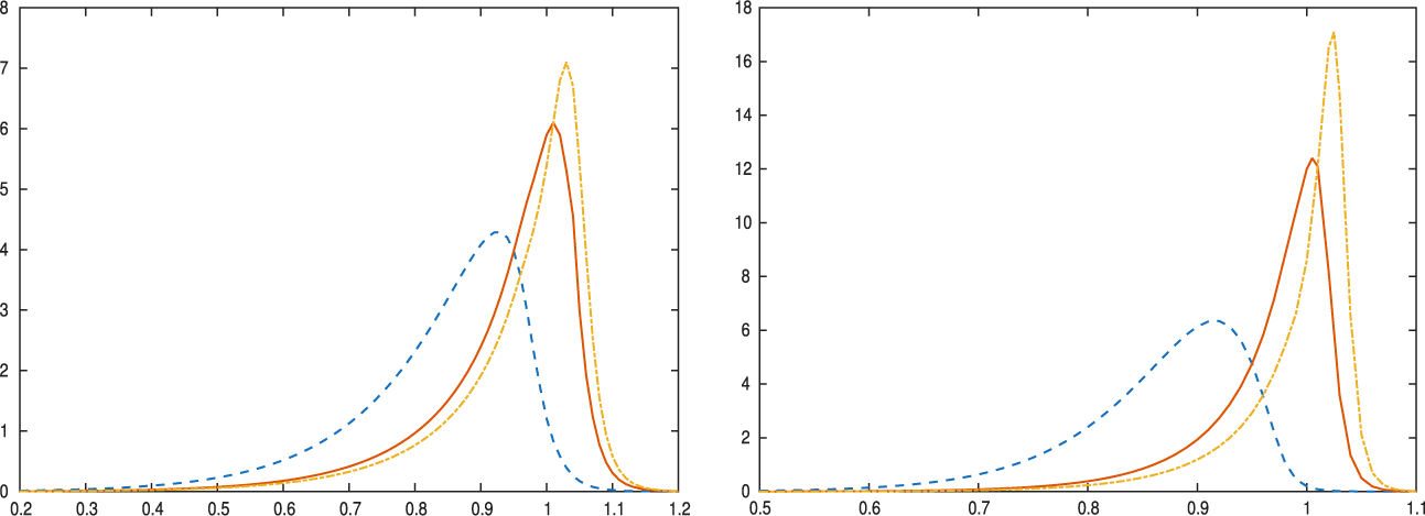


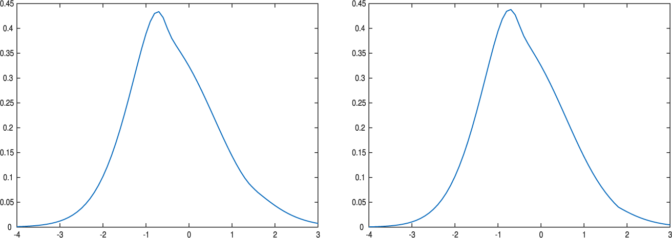


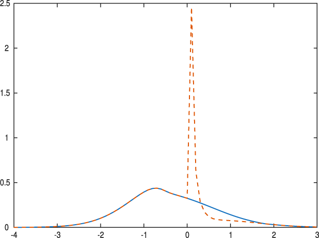


 Open access