





Impact statement
The manuscript presents an artificial intelligence-based methodology for defining overall crack patterns in structural elements of existing reinforced concrete (RC) bridges, enabling the characterization of features like counting and orientation, after detection. The article provides the pipeline of a near-complete tool, named DOC-Crack (DOC stands for detecting, orienting, counting), characterized by different novel sub-modules to (i) postprocess a stack of photos to define a comprehensive view of the structural element under investigation; (ii) define, test, and apply combined object detection and segmentation algorithms to recognize cracks; (iii) derive key features of crack pattern, that is, orientation (horizontal, diagonal, and vertical) and counting. The application of the tool to a real-life case study shows that the obtained results, which can strongly support structural engineering domain experts in assessing the current state of existing bridges through visual inspections, allow for predicting possible future issues related to crack evolution and to plan related interventions with a view to risk mitigation. The obtained outcome shows that the proposed tool is set to determine finer evaluation than existing approaches and to characterize a complete crack pattern, showing the precise extent of the defects over the entire structural elements.
1. Introduction
The maintenance of existing bridge portfolios is a primary issue addressed to public institutions, which need to ensure the safety of their infrastructures in order to prevent the repetition of past disasters (e.g., the collapse of the Polcevera Viaduct (Bazzucchi et al., Reference Bazzucchi, Restuccia and Ferro2018; Calvi et al., Reference Calvi, Moratti, O’Reilly, Scattarreggia, Monteiro, Malomo, Calvi and Pinho2019) that have caused irreparable losses. Usually, bridges are subjected to multiple sources of hazards, such as seismic actions (Nettis et al., Reference Nettis, Iacovazzo, Raffaele, Uva and Adam2022), geological movements (Nettis et al., Reference Nettis, Massimi, Nutricato, Nitti, Samarelli and Uva2023; Calò et al., Reference Calò, Ruggieri, Nettis and Uva2024), floods (Anisha et al., Reference Anisha, Jacob, Davis and Mangalathu2022), or natural decay of materials (Nettis et al., Reference Nettis, Nettis, Ruggieri and Uva2024). Therefore, the definition of the safety of existing bridges must be approached as a multirisk problem, following specific protocols, driving road management companies to employ reliable risk mitigation strategies. Taking as a reference the Italian case, the Ministry of Transportation, supported by the scientific community, developed and released new specific guidelines for the management and evaluation of the safety of existing bridges (MIT, 2021). These latter are characterized by a multilevel approach aimed at evaluating the health state of national bridge portfolios first, and then identifying the worst cases to employ specific interventions. The proposed approach involves six levels of assessment, each with different degrees of detail and complexity. The first three levels (Levels 0, 1, and 2) focus on a preliminary screening of bridge portfolios and are elaborated for defining prioritization lists, while the second three levels (Levels 3, 4, and 5) drive actions for bridges presenting higher risk in the earlier phases.
In this framework, one of the most significant phases is Level 1, during which onsite inspections of bridges are performed to assign an overall health score based on a detailed visual inspection of structural elements, including decks, girders, piers, bearings, and abutments. In this phase, the potential impact of various risk sources, including traffic, floods, landslides, and earthquakes, is also evaluated. The above tasks are addressed by trained surveyors, who conduct onsite inspections to record observed defects, including their intensity and extent, using a specific form. To complete the assessment, surveyors assign a score and take photographs, with the aim of tracking the evolution of each defect over time (i.e., by performing periodic inspections). On the one hand, the onsite visual inspection is a direct and practical method for detecting defects; on the other hand, several issues can impact the reliability of the final evaluation. In fact, one major issue is the subjective interpretation of defects by surveyors, which can be affected by human factors, such as attention lapses and fatigue, especially when dealing with a large number of bridges in a short time. In addition, external conditions, such as weather, lighting, and the distance between the surveyor and the inspected element, can also introduce uncertainties in defect scoring.
The matter becomes more complicated when assessing cracks, considering this type of defect is more difficult to survey and, at the same time, extremely important for defining the structural health of existing bridges. In this context, crack patterns are of interest and can be defined as the arrangement, shape, orientation, and distribution of cracks on the surface of the structural element. In other words, a crack can be visually considered the spatial aggregation of structural discontinuities detected on a concrete surface; from the perspective of an automated computer vision (CV) system, a crack is a continuous cluster of connected foreground pixels identified by a binary segmentation mask. The assessment of the evolution over time of crack patterns can be considered the most intuitive form of damage assessment and provides insights into the structural strength and durability of RC structures. Different aspects should be considered when discussing cracks and their related patterns. Given a generic RC structural element, the first aspect to address is the number of cracks, which reveal the extension of the defect within the element. Afterward, the extent of each crack should be assessed by evaluating its width and length to define the deterioration state of the structural element. Finally, another important aspect concerns the orientation of cracks (e.g., horizontal, vertical, and diagonal), which can reveal the causes of their formation and enable planning further action to minimize potential risks. By juxtaposing the above information, a general understanding of the problem can be developed by defining an overall crack pattern, which can provide insights into ongoing phenomena.
On this basis, it is clear that there is a need to develop new tools that support surveyors during onsite inspections, and in particular to aid in the characterization of the most delicate defects, such as cracks (Spencer et al., Reference Spencer, Hoskere and Narazaki2019). This paper addresses this issue by proposing a tool, DOC-Crack, an artificial intelligence (AI)-based framework for detecting, orienting, and counting cracks (according to the proposed acronym) in existing RC bridges. In detail, the proposed approach involves taking a stack of photos of the structural element to be inspected (e.g., using a high-resolution camera or an unmanned aerial vehicle, UAV) and stitching them to create a near-complete panoramic image of the element. Afterward, a DL pipeline is proposed to accurately detect the defective regions and segment their traces. By analyzing such traces across the stitched panorama, the framework extracts the complete crack pattern, enabling the automated counting and orientation assessment of all cracks. The proposed method was developed as a supervised DL approach, for which the authors collected and labeled a dataset by hand. DOC-Crack was developed and tested on a real case study, showing the high potential of the tool in supporting the onsite operations of surveyors and driving future actions for disaster prevention.
Overall, the main novelties of the proposed approach are the following.
-
• First, the modular integration of a stitching algorithm allows for the investigation of cracks over the entire structural element rather than confining the analysis to limited parts of specific images. Consequently, this enables inspection of composite image collections representing large structural elements of RC bridges, resulting in fewer distortions and artifacts.
-
• The framework adopts a modular approach to object detection and segmentation. Therefore, both the detection and segmentation modules can be replaced if required. Subsequently, a novel segmentation approach was developed to precisely trace the cracks. Specifically, starting from the bounding box returned from the detector, the segmentation module employs a pixel-level binary classification to identify thin cracks. This explicitly preserves the highest spatial resolution, preventing the loss of ultra-thin, continuous crack topologies that often disappear during the aggressive max-pooling and downsampling stages of standard encoder–decoder networks such as U-Net.
-
• The computation of crack orientation assumes paramount importance, serving as an effective tool to support domain experts in assessing the current condition of the structural elements.
It is important to emphasize that the novelty lies mainly in the end-to-end integration and workflow application. In other words, the main contribution lies in developing a modular framework that provides a structural mapping from raw UAV imagery. By integrating CV and DL, the proposed pipeline translates pixel-level predictions into meaningful insights, providing users with a comprehensive view of the structural health of RC bridges and serving as an effective decision-support system.
The rest of the paper is organized as follows: Section 2 reports the background about cracks characterization through CV-based approaches; Section 3 proposes the complete description of DOC-Crack; Section 4 reports the numerical experiments for training the proposed methodology; Section 5 proposes the application of DOC-Crack for a real case study; Section 7 provides the conclusions and the further developments.
2. CV-based approaches for characterizing cracks in RC elements
The characterization of cracks in RC structures is a fairly discussed topic in scientific literature, which in the last decades has proposed and developed several methodologies for detecting cracks from images and extracting specific information for better characterizing structural conditions. Generally, several methodologies to detect cracks could be mentioned, such as ultrasonic waves, stereoscopic camera systems, or laser scanners (Ding et al., Reference Ding, Yang, Yu and Shu2023). Nevertheless, of interest for the aim of this paper is to provide a background about CV approaches for the identification of cracks in RC structures directly from images, objects, and pixels. In this field, four main approaches can be mentioned: classification, segmentation, feature detection, and object detection (Di Mucci et al., Reference Di Mucci, Cardellicchio, Ruggieri, Nettis, Renò and Uva2024; Guo et al., Reference Guo, Liu, Xiao, Deng and Wang2024; Laflamme et al., Reference Laflamme, Blasch, Ubertini, Liu, Wertz, Knott, Cherry, Lindgren, Chang, Kumar, Poole, Worden, Downey, Wei, Musgrave, Wong, Quaranta, Rosso, Marano, Chen, Ardiles-Cruz, Soleimani-Babakamali, Avci, Inman, Taciroglu, Dodson, Chen, Meng, Zhu, Liu, Zuo, Liu, Khan, Hu, Hu, Cicirello, Cross, Chatzi, Weng, Yuan, Wen, Han, Metaxas, Tronci, Moaveni, Chen, Ng, Hackl, Chen, Wei, Mitoulis, Izonin, Uva, Ruggieri, Mao, Kiranyaz, Devecioglu, Gabbouj and Mohammadi2026).
Classification consists of categorizing objects or patterns in images according to some predefined classes. The aim is to define and assign a specific class to an input image or to a part of it. For example, Liang (Reference Liang2019) proposed a three-level image-based approach for performing classification and localization of damages in RC bridges, focusing on data derived from postdisaster inspections. Kim et al. (Reference Kim, Sim and Spencer2022) proposed a classification method to map crack pixels on images taken from smartphones and accounting for different angles, with the aim of characterizing the localization of cracks.
More suitable for detecting crack features in RC bridges is the segmentation, which is an approach in which the image is subdivided into multiple segments, with the aim of simplifying the identification of the regions to define in the image. Generally, segmentation allows the location of objects and the definition of boundaries in the focused image. In this regard, Li et al. (Reference Li, Zhao and Zhou2019) proposed a segmentation approach for proposing a multidefect detection (among which are cracks) based on pixel-level through the development of a fully convolutional network. A database of 2.750 images was collected, and the proposed approach achieved an accuracy of 98%. Saleem et al. (Reference Saleem, Park, Lee, Jung and Sarwar2020) proposed an approach exploiting instance segmentation through DL to localize and classify cracks in bridges, by using inspection images from UAVs. Ding et al. (Reference Ding, Yang, Yu and Shu2023) developed an approach using UAV surveys to detect and quantify cracks in RC without reference markers and using an independent boundary refinement transformer. Deng et al. (Reference Deng, Sun, Yang and Cao2023) proposed a three-dimensional (3D) crack mapping to localize cracks in a surface by using a point cloud model developed on a video-based reconstruction. Chu et al. (Reference Chu, Wang and Deng2022) proposed Tiny-Crack-Net, a multiscale feature fusion network with attention mechanisms to solve the problem of class imbalance in crack segmentation. The proposed approach achieved an accuracy of 91% for cracks with a width of 0.05 mm. Other works using segmentation can be mentioned for the sake of brevity, such as Wang and Su (Reference Wang and Su2022), Kang and Cha (Reference Kang and Cha2021), Wang et al. (Reference Wang, Zhai, Huang, Guan, Mu and Wang2020).
Another approach for crack definition is feature detection, which allows identifying and locating patterns (i.e., features) in the focused images. The approach is suggested for defects like cracks, since feature detection can identify both simple lines and complex figures. If applied in different moments, feature detection can also allow for investigating the variations of defects over time. For example, Liu et al. (Reference Liu, Nie, Fan and Liu2019) proposed an image-based crack method aimed at extracting features from bridge piers by using a UAV and 3D scene reconstruction. From the proposed method, the authors were able to define the shape of the cracks and the related width, with negligible errors.
The last and more recent CV-based method for cracks (and defects) characterization is object detection, able to recognize objects in images. In fact, it consists of identifying, localizing, and classifying the desired object within the image. Two main kinds of object detectors are widely spread in practice: (a) two-stage object detectors, which present two neural networks able to identify and classify, respectively, objects in the image; (b) single-stage detectors, which adopt a single network to address both localization and classification tasks. Regarding cracks in RC elements, Yu et al. (Reference Yu, Shen and Shen2021) proposed a real-time detection of cracks in bridges by combining the potentialities of UAVs and a modified version of YOLOv4. This latter was modified by using focal loss to optimize the loss function. The above modification improved accuracy, achieving 97.6%. Cha et al. (Reference Cha, Choi and Büyüköztürk2017) proposed a convolutional neural network (CNN) based on a sliding window technique for detecting cracks, showing an overall accuracy of 98% by training the network on 40.000 images. Deng et al. (Reference Deng, Lu and Lee2020) proposed a version of a Faster R-CNN on a dataset constituted by 5.000 images to detect cracks in RC bridges, accounting for interferences due to handwriting automatically. The obtained results were compared with those obtained by YOLOv2, showing several advantages in terms of accuracy. Park et al. (Reference Park, Eem and Jeon2020) used YOLOv3 in a real-time defect detection of cracks in RC structures, for characterizing the size and position of the considered defect. The results of experiments demonstrated high accuracy (about 94%) and precision (about 98%). Other works can be mentioned about the use of object detection for cracks, such as Yu et al. (Reference Yu, Shen and Shen2021), Jiang and Zhang (Reference Jiang and Zhang2019), but it is worth noting that most of the above works, although present approaches with high accuracy, are mainly focused on the characterization of single cracks (also very thin) and usually exploit single images given by onsite inspections.
Instead, the proposed approach, DOC-Crack, potentially leads to a major advance in the field of crack detection, providing an end-to-end framework to reconstruct the complete crack pattern in RC structural elements, starting from unlabeled imagery directly gathered in the field. In other words, DOC-Crack extracts a complete semantic assessment of the status of the RC structural element, providing the domain expert with human-readable information to localize, count, and estimate the orientation of each crack. To achieve this goal, DOC-Crack was engineered as an end-to-end framework that exploits a modular pipeline to provide the desired information from the imagery of the RC structural element under investigation.
3. DOC-Crack: Definition of the methodology and description of sub-modules
This section presents DOC-Crack, describing the proposed submodules with the related datasets and algorithms. The framework of DOC-Crack is shown in Figure 1, which reports the complete processing pipeline at the base of the method.
The DOC-Crack framework. Once a dataset is gathered and prepared for training, a detection network based on stable iterations of YOLO is trained. Then, during inference, partially overlapped images of RC bridges are stitched together, and a method containing an object detection pipeline, followed by an instance segmentation tool, is used to provide a preliminary assessment of the cracks within the RC bridge.
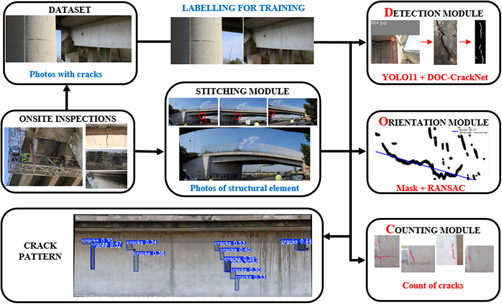
Figure 1. Long description
A flowchart organized into several functional blocks connected by arrows.
1. Data Acquisition (Left Column):
- Onsite Inspections: Shows photos of workers on a lift under a bridge and close-ups of concrete damage. An arrow points up to Dataset and right to Stitching Module.
- Dataset: Contains photos with cracks. An arrow points right to Labelling for Training.
2. Processing (Center):
- Labelling for Training: Shows bridge photos with highlighted crack regions. An arrow points right to the Detection Module.
- Stitching Module: Labeled Photos of structural element, showing three overlapping bridge photos being combined into a single panoramic view. An arrow points right to the analysis modules.
3. Analysis Modules (Right Column):
- Detection Module: Labeled Y O L O 11 plus D O C-Crack Net. Shows a sequence from a raw bridge photo to a cropped crack image and finally a binary black-and-white crack mask.
- Orientation Module: Labeled Mask plus R A N S A C. Displays a scatter plot of crack pixels with a blue linear regression line indicating crack angle.
- Counting Module: Labeled Count of cracks. Shows four small cropped images with red lines tracing individual cracks.
4. Output (Bottom):
- Crack Pattern: A large final image of a bridge wall with blue bounding boxes and numerical labels (e.g., cracks 0.47, cracks 0.53) identifying and assessing multiple crack locations. Arrows from the three analysis modules on the right converge and point back to this final block.
The main steps are briefly summarized, and are accurately described in the next Sections:
-
1. Onsite inspection and dataset collection: to perform onsite surveys by domain experts on structural elements. Ideally, the surveyor should take photos in a specific way, only possible by exploiting proper equipment, such as UAVs. Still, to collect additional data to train the automatic algorithms of detection, an existing database or other photos (i.e., closer to cracks) should be collected.
-
2. Stitching: the collected photos are elaborated through a stitching procedure, providing a comprehensive view of the structural element under investigation.
-
3. Labeling: the collected dataset must be labeled for the purpose of CV algorithms. In particular, the labeling should identify the exact trace of cracks.
-
4. Crack detection, counting, and segmentation: parts of the image containing cracks are detected and counted by using specific object detectors based on YOLO (Redmon et al., Reference Redmon, Divvala, Girshick and Farhadi2016), and trained on the above dataset to improve the efficiency of the algorithm. Once the crack is identified, a novel segmentation technique is employed to accurately define the crack patch.
-
5. Crack pattern and orientation: the identified cracks can be relocated on the initial stitched image to define the crack pattern. In addition, the orientation feature can be estimated by exploiting a pixel-level evaluation procedure.
3.1. Onsite inspections and data collection
The first phase of the proposed procedure consists of performing onsite inspections, aimed at collecting data. Two types of data need to be gathered: (a) photos of the structural elements to be analyzed in DOC-Crack; (b) photos of cracks from different views to enrich the overall dataset for the training.
Concerning the first type of data, once the structural element to investigate is identified, two simple approaches could be exploited: (a) use of a UAV; (b) a human survey with a high-resolution camera. When using UAVs, a specific protocol should be followed. In particular, once the absence of obstacles has been assessed, the UAV performs the flight following a series of reference points. The latter are designed to create a virtual fence area, which the UAV follows according to a linear route, parallel to the longitudinal development of the structural element. The distance from the UAV to the structural element is estimated according to the optical cone of the machine and its resolution, by ensuring an overlap between consecutive photos of at least 30% and ensuring the same angle (as suggested in Wang et al. (Reference Wang, Demartino, Narazaki, Monti and Spencer2023)). Similar performance could be achieved through a high-resolution camera managed by human surveyors, as indicated above. Nevertheless, although this second option may be cheaper than the first, it is strongly influenced by the presence of obstacles (e.g., vegetation), the photographer’s skill, and the height of the structural element being investigated (i.e., the deck and its components). A possible solution to the above issues is represented by the by-bridge platform.
Regarding the second type of data, a consistent dataset of defects on different structural elements must be collected, for example, (Cardellicchio et al., Reference Cardellicchio, Ruggieri, Nettis, Renò and Uva2023; Ruggieri et al., Reference Ruggieri, Cardellicchio, Nettis, Renò and Uva2023, Reference Ruggieri, Cardellicchio, Nettis, Renò and Uva2025), ensuring that the minimum requirements for the subsequent steps are met. In particular, the collected dataset should be characterized by (a) scale, (b) diversity, and (c) quality. Regarding scale, as reported by Cardellicchio et al. (Reference Cardellicchio, Ruggieri, Leggieri and Uva2022), a consistent size of dataset, characterized by several examples and typology of defects, should be collected. In addition, data balance should be ensured. Concerning diversity, the dataset should be characterized by enough intra- and inter-class variations, that is, each feature should be described by data accounting for variation of appearance, position, viewpoint, and pose, without discarding images with noise and occlusions. Finally, high-quality images are required, since low-resolution data can negatively influence the accuracy of the detection models.
3.2. Robust image stitching for global bridge view
Limitations of the sensing equipment, mainly in terms of field of view and resolution, imply that a single, comprehensive view containing the structural element to monitor is often not gathered in a single image. Therefore, providing a robust and reliable stitching procedure is a mandatory prerequisite for analyzing large-scale defects and assessing the overall structural health status. To this end, this work incorporates a well-assessed, feature-based stitching methodology, whose results are shown in Figure 2.
An example of image stitching. First, key points are located using the Harris detector. Then, invariant descriptors are extracted and matched for each key point to identify overlaps between images. Finally, the panorama is obtained using a warping transformation.
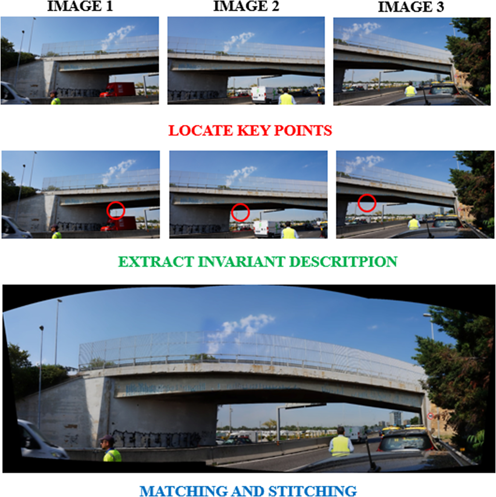
The pipeline begins by detecting and describing keypoints by means of a Harris corner detector (Harris et al., Reference Harris and Stephens1988), and local invariant descriptors, such as Scale-Invariant Feature Transform (SIFT) (Lowe, Reference Lowe2004), which were computed to match features reliably between partially overlapping images. Once possible matching points are computed, the Random Sample Consensus (RANSAC) algorithm (Fischler and Bolles, Reference Fischler and Bolles1981) was used to estimate a homography matrix. The primary motivation for the selection of RANSAC is its robustness to outliers, which ensures that the estimated homography is based on geometric consensus, thus minimizing misalignments. Finally, the starting images were warped according to the homography matrix and blended to create a seamless overall view of the structural element.
3.3. Dataset and preparation for detection algorithms training
The data collected following the procedure highlighted in Section 3.1 were used to create two different datasets. The first dataset, the large-scale defect dataset, was used to train a deep neural network for the crack detection task, that is, localizing areas of interest within the images where a crack is likely to be found. The second dataset, the high-precision crack segmentation dataset, was then used to train another neural network to perform semantic segmentation, thereby identifying cracks within the areas of interest identified by the detection algorithm.
3.3.1. Dataset for large-scale defect detection
This dataset was used for training a DL object detector to identify several classes of damage. The dataset was composed of 10.779 images, which were manually labeled by domain experts using the Computer Vision Annotation Tool (CVAT) (Sekachev et al., Reference Sekachev, Manovich, Zhiltsov, Zhavoronkov, Kalinin, Hoff, Osmanov, Kruchinin, Zankevich, Markelov, Chenuet, Melnikov, Kim, Ilouz, Glazov, Tehrani, Jeong, Skubriev, Yonekura and Truong2020). Specifically, the labeling was performed to deal with the damage detection task; therefore, the outcome was in the form of bounding boxes. The labeling allowed the identification of seven types of different defects, which were used to provide multiple damage detection (Ruggieri et al., Reference Ruggieri, Cardellicchio, Nettis, Renò and Uva2024; Ruggieri et al., Reference Ruggieri, Cardellicchio, Nettis, Renò and Uva2025).
3.3.2. Dataset for high-precision crack segmentation
The dataset for training the segmentation network originated from a set of 450 images, specifically selected for their high-quality representation of crack defects. This dataset was labeled by domain experts by hand-tracing the full extent of visible cracks. Also in this case, the CVAT tool was used, and the results were exported in the Dataset Management Framework (Datumaro) format (Datumaro, 2022).
After labeling, a patch-based generation method was exploited to create the training samples for the pixel-wise classifier. Specifically, a square filter of size
$ F $
 was used to extract a patch at each pixel location; each of these patches was then labeled as either a crack or a noncrack sample, based on the fact that its central pixel belonged to a crack or not. These generated
$ M\times N\times 450 $
was used to extract a patch at each pixel location; each of these patches was then labeled as either a crack or a noncrack sample, based on the fact that its central pixel belonged to a crack or not. These generated
$ M\times N\times 450 $
 data samples where
$ M\times N $
data samples where
$ M\times N $
 was the size of each image. Thus, this approach addresses data scarcity by generating data directly from the source pixel rather than through image-processing transformations, thereby mitigating the risk of overfitting. However, this process implied a severe class imbalance, with the noncrack images vastly outnumbering the crack samples. As such, a hard-negative mining sampling strategy was implemented to balance the data and improve performance.
Still, before generating the patches, the 450 images were randomly split into two distinct sets, namely a training and a validation set, using a 70−30 split. This was specifically designed to prevent data leakage and thereby improve the overall generalization capabilities of models trained on the dataset. Overall, this resulted in three datasets of roughly the same size, as detailed in Table 1.
Datasets created for high-precision crack segmentation

Table 1. Long description
The table consists of three columns and four rows including the header.
* Header Row: Image patch size, Number of crack patches, and Number of noncrack patches.
* Row 1: Image patch size 64 times 64. Number of crack patches is 195.971. Number of noncrack patches is 198.656.
* Row 2: Image patch size 128 times 128. Number of crack patches is 195.813. Number of noncrack patches is 198.656.
* Row 3: Image patch size 256 times 256. Number of crack patches is 194.376. Number of noncrack patches is 198.656.
A note below the table explains that noncrack patches are negatively undersampled for balance, and larger patch sizes yield slightly fewer crack samples because no padding was applied to border patches.
Note. The noncrack patches are negatively undersampled to provide a balanced dataset. The number of crack patches varies with the size of the considered patch; as expected, larger patches yield slightly fewer data samples. No padding was applied as border patches were not considered.
3.4. Crack detection and counting
The enabling step in the processing pipeline was provided by the object detection model, which was specifically trained to identify multiple defects within imagery representing structural elements of RC bridges. To this end, starting from the work in Ruggieri et al. (Reference Ruggieri, Cardellicchio, Nettis, Renò and Uva2025), two variants on the basic architecture of YOLO11 Jocher and Qiu (Reference Jocher and Qiu2024) were proposed. Specifically, the YOLO family was originally proposed by Redmon et al. (Reference Redmon, Divvala, Girshick and Farhadi2016) as a single-stage object detector, that is, a DL model capable of localizing and classifying objects of interest within an image using a single CNN. In Ruggieri et al. (Reference Ruggieri, Cardellicchio, Nettis, Renò and Uva2025), the concept of Convolutional Block Attention Module (CBAM) was applied to the neck of YOLO11, highlighting improved detection capabilities for the network. While improving the overall performance of the network, the use of CBAM poses some constraints; specifically:
-
• Feature Interaction Limitations: CBAM decouples attention into the channel (i.e., monodimensional) and spatial (i.e., bidimensional) components. While effective, this approach prevents the capture of true 3D attention weights, which are given by relationships between the spatial dimensions and the channels. Consequently, distinctive features restricted to specific spatial locations or feature channels may be suppressed due to the global pooling performed by the CBAM attention, potentially leading to information loss.
-
• Reliance on Heuristics and Parameters: The CBAM module was designed around a set of heuristics, such as specific kernel sizes and reduction ratios in its multilayer perceptron (MLP), thus introducing additional hyperparameters and computational overhead, increasing the complexity of model tuning and inference.
To address these issues, two attention mechanisms were separately explored. First, the Global Attention Mechanism (GAM) introduced in Liu et al. (Reference Liu, Shao and Hoffmann2021) was considered to address the limitation of feature refinement by focusing on retaining information across dimensions to strengthen interactions. The main innovation behind the GAM lies in its design, which minimizes information reduction while maximizing cross-dimensional feature interaction to enhance global interactive representation. GAM achieves this by utilizing sequential submodules, notably in its Channel Attention submodule, where the input tensor is permuted and then processed by an encoder–decoder MLP to learn channel-spatial dependencies.
The second explored mechanism was SimAM, introduced by Yang et al. (Reference Yang, Zhang, Li and Xie2021), which leverages a fundamentally different approach inspired by neuroscience principles, allowing for the calculation of full 3D attention weights in an efficient, parameter-free manner. Specifically, the SimAM mechanism is derived from the neuroscientific theory of spatial suppression, which states that the most informative neurons are those that display distinctive firing patterns within a neighborhood and, therefore, should be prioritized. To this end, SimAM computes the importance of a single target neuron n by defining an energy function
$ {e}_n $
 that measures the linear separability between n and its neighbors. A lower energy value indicates that the neuron is more distinctive and, therefore, more important for visual processing; consequently, the attention weight is computed as the inverse of the energy
$ \sigma \left(1/{e}_n\right) $
that measures the linear separability between n and its neighbors. A lower energy value indicates that the neuron is more distinctive and, therefore, more important for visual processing; consequently, the attention weight is computed as the inverse of the energy
$ \sigma \left(1/{e}_n\right) $
 .
.
Two specific sections of the YOLO11 original network were targeted by the insertion of these mechanisms, namely the backbone and the neck. As for the backbone, two reasons underlie this choice: the first is to provide a mechanism that forces the network to recalibrate feature weights early on during training, effectively dimming the background and non-relevant information while highlighting the foreground elements of the image. Another effect is a prioritization of the channels that respond to specific spatial frequencies, such as the edge of a crack, over generic texture channels. Regarding the neck, it is worth noting that this section of the network combines semantic features extracted at various abstraction levels, enabling multiscale detection. Inserting attention mechanisms in this part of the network helps in achieving two goals: first, when features from a deep layer are concatenated with those from a shallow layer, a semantic gap can arise; attention mechanisms can help in deciding which details from the shallow layer are actually relevant to the semantic representation provided in the deep layer. Second, since deep layers inherently lose spatial precision, inserting attention in the neck helps recover precise defect localization from the shallow layers.
The models were first trained from scratch on the detection dataset, split according to a 70−30 strategy. Consequently, the trained models could be used to localize cracks within the input imagery, allowing for the estimation of defect positions within the final stitched image. In addition, the use of the object detector enables the counting of the number of occurrences of the defect. To this end, a counting module was implemented to quantify all cracks across the stitched image, thereby evaluating the extent of the crack pattern.
3.5. Crack segmentation
Once the cracks were detected using the best-performing object detection model, a novel pixel-based approach was developed to estimate the pattern of the identified cracks. This approach was based on a specifically designed neural network, named DOC-CrackNet, aimed at framing the problem in a different and possibly simpler way. Specifically, instead of using classic segmentation approaches based on U-shaped networks, the idea was to frame the problem as a binary classification problem, thereby training a simple CNN to distinguish between areas whose center likely belongs to a crack and areas whose center does not. This allowed three main improvements over other existing approaches:
-
1. The problem of data availability was solved, as it was possible to extract a large number of patches from a starting image. Ideally, given an image of $ M\times N $
 pixels, the proposed approach could extract up to
$ \left(M- fracW2\right)\times \left(N- fracW2\right) $
different patches, where
$ W $
represents the size of the selected patch. This allowed an exponentially higher number of samples to populate the dataset for the investigation.
pixels, the proposed approach could extract up to
$ \left(M- fracW2\right)\times \left(N- fracW2\right) $
different patches, where
$ W $
represents the size of the selected patch. This allowed an exponentially higher number of samples to populate the dataset for the investigation. -
2. The problem of interpretability was partially mitigated by the adoption of simpler models, such as the one used in this work, which was composed of only three stacked simple convolutional layers.
-
3. Framing the problem as a binary classification allowed a probabilistic output that, in future works, can be exploited to further improve the overall results of the network by adopting a flexible, variable classification threshold.



Interestingly, it must also be noted that exploiting simpler models allows for the reduction of the overall computational weight of the network, potentially enabling the adoption of this approach even on constrained hardware in real-time. The feature map size-halving criteria established by (He et al., Reference He, Zhang, Ren and Sun2016) was followed to design DOC-CrackNet. The network scheme of DOC-CrackNet is shown in Figure 3.
The architecture of the proposed network. Specifically, DOC-CrackNet accepts an RGB image of the desired size (in this case
$ 64\times 64 $
 ). The image is then fed to three consecutive convolution layers, after which it is reduced in size using a max pooling layer. Finally, a fully connected layer extracts a feature embedding vector of 576 elements, fed to a sigmoid classifier for the final decision.
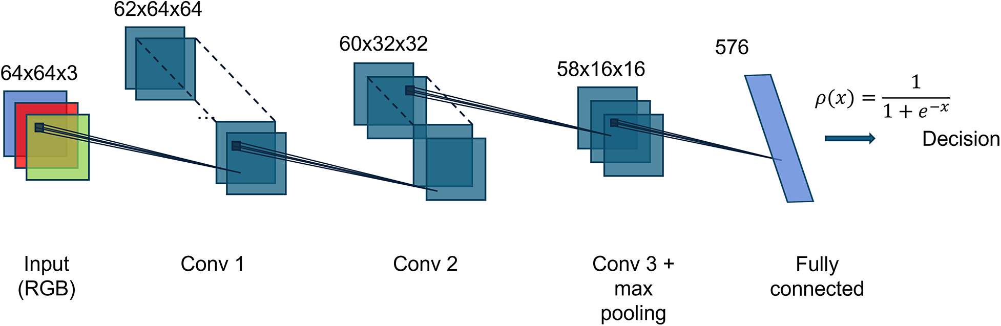
Figure 3. Long description
The diagram illustrates a neural network pipeline consisting of five main stages from left to right.
* Input (R G B). Three overlapping colored squares (red, green, and blue) labeled 64 times 64 times 3. Solid lines connect a small kernel area to the next stage.
* Conv 1. A stack of blue feature maps labeled 62 times 64 times 64. Dotted lines indicate a spatial reduction or transformation process.
* Conv 2. A stack of blue feature maps labeled 60 times 32 times 32. Solid lines connect a kernel from this layer to the next.
* Conv 3 plus max pooling. A stack of blue feature maps labeled 58 times 16 times 16. A single line connects this stack to the next layer.
* Fully connected. A single vertical blue bar labeled 576. To its right is the sigmoid activation function equation rho of x equals 1 all over 1 plus e to the power of minus x.
A final arrow points from the equation to the word Decision at the far right.
The latest layer of DOC-CrackNet presents a sigmoid activation function, which was chosen over the softmax activation function as the problem is framed as a binary classification task. In other words, through the sigmoid activation function, DOC-CrackNet provides a probability value
$ \sigma \in \left[0,1\right] $
 representing the likelihood that the patch is a positive (i.e., it represents a crack) or a negative sample (i.e., it does not represent a crack). This evaluation requires fixing a threshold value
$ \phi $
representing the likelihood that the patch is a positive (i.e., it represents a crack) or a negative sample (i.e., it does not represent a crack). This evaluation requires fixing a threshold value
$ \phi $
 to distinguish between the two different cases and to provide the metrics used for the overall performance evaluation:
-
• True Positives (TP): the number of patches whose central pixel represents a crack and is correctly classified as a positive sample.
-
• True Negatives (TN): the number of patches whose central pixel does not represent a crack and is correctly classified as negative samples.
-
• False Positives (FP): the number of patches whose central pixel does not represent a crack and is incorrectly classified as a positive sample.
-
• False Negatives (FN): the number of patches whose central pixel represents a crack and is incorrectly classified as a negative sample.
The threshold is manually set using threshold-moving (Provost, Reference Provost2000) to maximize the value achieved by the F1 score, defined as:
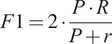
where
$ P $
 represents the precision, defined as:
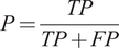
while
$ R $
 is the recall, defined as:
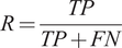
Therefore, higher precision is achieved when the model can misclassify a few negative samples, while higher recall is achieved when the model can misclassify a few positive samples. The F1 score synthesizes these aspects within a single metric.
The outcome of this step is a binary estimation mask
$ M $
 , whose value is white for the points where the crack is identified and black otherwise. This allows for identifying and segmenting each crack within the original images, delineating its pattern within the structural element.
Finally, it is worth underlining that the structure of DOC-CrackNet was designed to be flexible enough to accept patches of different sizes as inputs, allowing the evaluation of the impact of contexts for different sizes on the overall performance of the network.
3.6. Estimation of main crack orientation
Assessing the principal orientation of a crack is a critical feature for structural health management. In other words, while cracks often exhibit complex, nonlinear geometries, providing a robust, first-order approximation of their dominant linear trend (e.g., horizontal, vertical, or diagonal) can provide important insights into the causes behind a certain defect, as well as future maintenance strategies that can be proven effective.
The orientation is estimated in a two-stage process. First, the binary segmentation mask
$ M $
 obtained after crack segmentation is preprocessed by applying a morphological erosion filter. This step filters out segmentation artifacts and spurious branches, therefore ensuring the analysis is performed on the main component of the crack.
Once the erosion filter was applied
$ M $
 , the resulting erosion mask
$ {M}_{er} $
, the resulting erosion mask
$ {M}_{er} $
 was used as an input to train a regressor by means of the RANSAC algorithm (Fischler and Bolles, Reference Fischler and Bolles1981). The motivation behind the use of RANSAC lies in the consideration that a simple linear regressor would estimate an overall trend that is extremely sensitive to outliers. Using a robust regressor would filter out residual segmentation noise, as well as the nonlinear portions of the crack, allowing for robust identification of the single best-fit line representing the dominant trend of the crack.
Once the optimal regression model
$ {R}_i $
 is computed using RANSAC, its coefficient is converted to an angle
$ \alpha $
is computed using RANSAC, its coefficient is converted to an angle
$ \alpha $
 and used to evaluate the direction of the crack according to the thresholds shown in Table 2. As can be observed, horizontal cracks are classified as ranging from 0° to 25°, diagonal cracks are classified as ranging from 25° to 60°, and vertical cracks are classified as ranging from 60° to 90°.
Threshold for determining the orientation of the crack according to the slope of the estimated model Ri

Table 2. Long description
The table consists of three columns: Orientation, Minimum value (degrees), and Maximum value (degrees). It contains three data rows:
* Horizontal: Minimum value 0, Maximum value 25.
* Diagonal: Minimum value 25, Maximum value 60.
* Vertical: Minimum value 60, Maximum value 90.
A footnote specifies that while only values between 0 and 90 degrees are shown, thresholds can be adapted to all scenarios by applying an offset of plus or minus pi all over 2.
Note. For the sake of simplicity, only values between
$ 0 $
 and
$ 90 $
and
$ 90 $
 degrees were considered. However, if an offset of plus or minus
$ \frac{\pi }{2} $
degrees were considered. However, if an offset of plus or minus
$ \frac{\pi }{2} $
 is applied to the specified values, the thresholds can be adapted to all the possible scenarios.
It is worth specifying that the proposed approach for estimating crack orientation is mainly based on the classification provided by the Italian guidelines MIT (2021), which subdivides cracks into the three classes defined above. Obviously, more complex crack shapes could be experienced in some real-life cases, for which the classes subdivision like the one provided could be too simplistic. Nevertheless, during onsite inspections, the domain expert must follow the guidelines and rules and then needs to assume a class within the three classes above defined. Still, although DOC-Cracks allows to detect and to trace also complex cracks, the logic behind the tool (not only with reference to orientation, but in the near-complete definition of crack pattern) is to support domain experts, who should always validate the output provided by the proposed automatic tool. Finally, it is clear that more complex approaches could be employed to define orientation (e.g., instance-level skeletonization to map varying orientations along the continuous path of a single curved crack), which are beyond the scope of this paper and can be the object of future developments.
4. Experimental section
In this section, the experiments performed to elaborate the steps of the framework are described. All the experiments were carried out by using a machine equipped with an Intel Core i9-14900HK, 64 GB of RAM, and an NVIDIA GeForce 4090 with 24 GB of VRAM. The experiments were performed using Python as the primary programming language and the PyTorch library (Paszke et al., Reference Paszke, Gross, Massa, Lerer, Bradbury, Chanan, Killeen, Lin, Gimelshein, Antiga, Desmaison, Köpf, Yang, DeVito, Raison, Tejani, Chilamkurthy, Steiner, Fang, Bai and Chintala2019) under a single-GPU configuration.
4.1. Training of object detector and automated crack segmentation
4.1.1. Full-scale RC bridge object detector
For the case at hand, the base dataset was gathered by following the procedure described in Cardellicchio et al. (Reference Cardellicchio, Ruggieri, Nettis, Renò and Uva2023); Ruggieri et al. (Reference Ruggieri, Cardellicchio, Nettis, Renò and Uva2023, Reference Ruggieri, Cardellicchio, Nettis, Renò and Uva2025). Specifically, a total of 10,779 images were acquired during surveys of the structural elements of existing RC bridges, mainly decks, piers, pier caps, and abutments. Most of the gathered images were related to one or more structural elements, showing several defects of different extents and intensities. According to the above-mentioned works, the first labeling was performed to identify seven types of defects related to RC bridges.
The results of testing different configurations of YOLO models with various attention mechanisms are detailed in Table 3. Crucial considerations can be made concerning how placing different attention mechanisms in different parts of the network influences its behavior.
Comparison of model performance across metrics
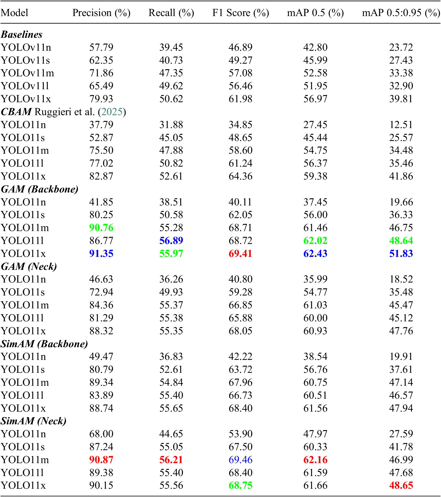
Table 3. Long description
The table compares performance metrics (Precision, Recall, F 1 Score, m A P 0.5, and m A P 0.5 to 0.95) for Y O L O v 11 variants (n, s, m, l, x) across six categories.
* Baselines: Y O L O v 11 x achieves the highest baseline F 1 Score at 61.98 percent.
* C B A M (Ruggieri et al. 2025): Y O L O 11 x leads this group with a Precision of 82.87 percent and F 1 Score of 64.36 percent.
* G A M (Backbone): Shows significant improvement. Y O L O 11 x reaches 91.35 percent Precision, 55.97 percent Recall, and 69.41 percent F 1 Score. Y O L O 11 l also shows high performance with 56.89 percent Recall and 62.02 percent m A P 0.5.
* G A M (Neck): Y O L O 11 x leads with 88.32 percent Precision and 68.05 percent F 1 Score.
* Sim A M (Backbone): Y O L O 11 m reaches 89.34 percent Precision, while Y O L O 11 x has an F 1 Score of 68.40 percent.
* Sim A M (Neck): High performance across the board. Y O L O 11 m achieves 90.87 percent Precision and 56.21 percent Recall. Y O L O 11 x reaches an F 1 Score of 68.75 percent and m A P 0.5 to 0.95 of 48.65 percent.
Bolded values indicate peak performance within specific categories, notably concentrated in the G A M Backbone and Sim A M Neck configurations for the larger model variants.
Note: Values in green indicate the best results, values in red the second-best, and values in orange the third-best.
Specifically, the integration of GAM within the backbone yielded an overall superior value for mAP 0.5:0.95 outperforming baseline architectures by approximately 2.4% when the largest model scale (YOLO11x) was considered. This implies that, by filtering background noise at the earliest stages of feature extraction, the model achieves higher robustness, resulting in a stronger, noise-free feature representation. This enhanced feature space enables the detection head to focus solely on structural defects, resulting in tighter, more effective, and precise bounding boxes. Another significant finding is that the insertion of SimAM within the neck resulted in the optimal F1 score for the medium-sized model, thus implying a better trade-off between precision and recall, with a top value of 69.46% . This therefore suggests that the 3D attention weights proposed by SimAM are effective during the multiscale fusion stage, allowing for reliable discrimination of true defects from complex textures.
It is worth framing the impact of the proposed architectural enhancements on different network sizes. Specifically, there is a larger contribution for smaller scales (i.e., nano and small), mainly with the parameters-free SimAM attention mechanism. This effectively compensated for the relatively limited capacity of such networks, showing relative improvements of nearly 15% when placed within the neck for YOLO11n. At the same time, the relative contribution of the attention mechanisms is less relevant (yet not negligible) for larger scales, mainly due to the high representation capability already embedded in those architectures. Consequently, a sweet spot can be determined for the medium-sized model, as demonstrated by the introduction of SimAM in the neck.
Overall, these findings suggest that using a combination of SimAM and GAM can provide further improvements and should be explored in future work.
4.1.2. Crack detection
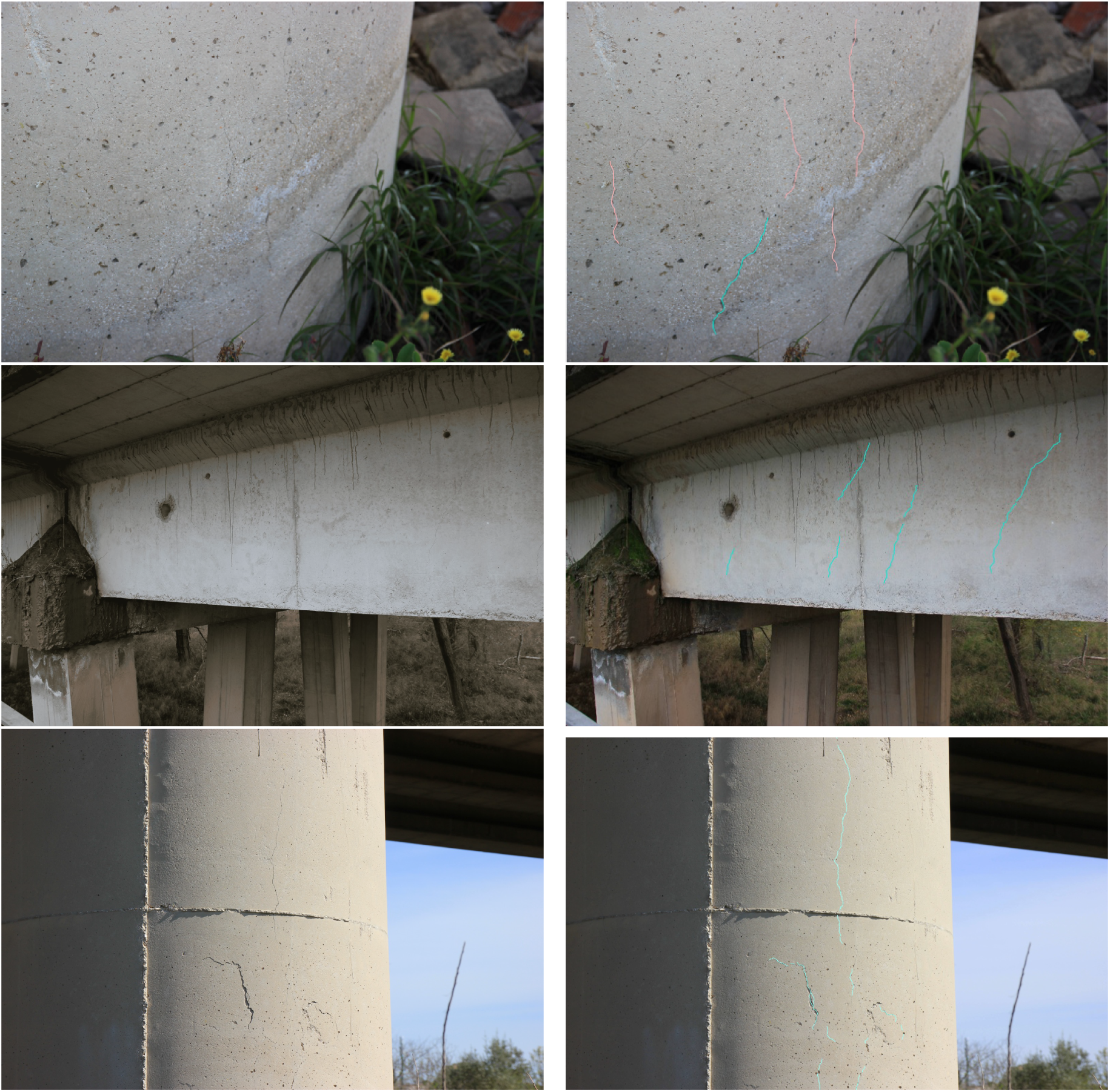
The trained model was fine-tuned to focus on cracks on the second, smaller dataset. This was characterized by 450 images containing visible samples of cracks. For each image of this new subsample, a further annotation was performed by hand-tracing cracks. Some examples of the new labeling, along with their corresponding ground truth, are shown in Figure 4.
On the right, the results of the labeling segmentation procedure on the image on the left are highlighted in light blue or pink.
According to the procedure defined in Section 3.4, crack patches were derived, and the resulting segmentation dataset was composed of 195.971 positive samples and 198.656 negative samples. Some of the results are shown in Figure 5, in which patches with and without cracks are reported.
A sample of the segmentation dataset. On the first row, six patches where cracks were not found are shown, while on the second row, six patches where cracks were found are reported.
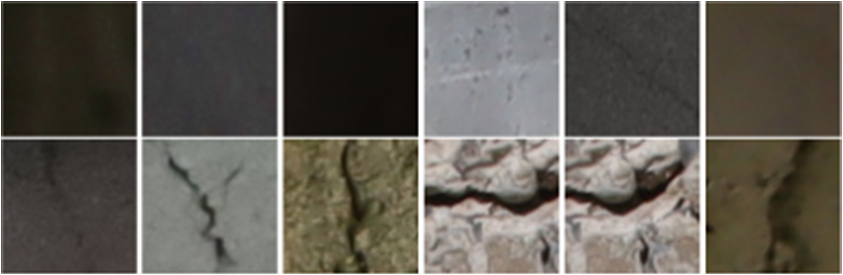
Figure 5. Long description
The top row contains six patches of uniform material surfaces without visible defects. These patches vary in color and texture, including dark brown, charcoal gray, black, light gray with minor pitting, medium gray, and tan.
The bottom row contains six patches exhibiting various types of structural cracks.
- The first patch on the left shows a faint, dark vertical hairline crack.
- The second patch features a prominent, jagged Y-shaped crack on a light gray surface.
- The third patch shows a deep, dark vertical fissure on a rough, yellowish-brown surface.
- The fourth and fifth patches are nearly identical, showing a wide, horizontal jagged crack with significant depth and shadow on a light, stony texture.
- The sixth patch on the far right shows a vertical crack along the edge of a tan-colored surface.
Subsequently, a data augmentation procedure was also considered, through a series of augmentation steps specifically tailored to retain the semantic meaning of each image. Specifically, random rotations around the central pixel, random flipping (both horizontal and vertical), and random adjustment in terms of sharpening, contrast, and saturation were considered. All the augmentation steps were designed to provide a larger variability of the data fed to the network while retaining the information provided by the central pixels of the patch, and then not varying its class.
As for the hyperparameters, binary cross-entropy was selected as the loss function, with SGD as the optimization algorithm and 25 epochs of training with a learning rate of 0.01. All these parameters were experimentally found to be optimal for the problem at hand. Finally, as for the size of the input patch, let us recall that, as already stated in Section 3.4, DOC-CrackNet was designed to be flexible enough to accept patches of different sizes as input. To test the influence of the contextual information at different scales, the tests were conducted using square masks of three different input sizes, that is,
$ 65\times 65 $
 ,
$ 129\times 129 $
,
$ 129\times 129 $
 , and
$ 257\times 257 $
, and
$ 257\times 257 $
 . These values were selected experimentally, considering the overall size of the images under investigation and the memory constraints of the hardware used during training. In the following, each version of DOC-CrackNet will be referred to using a suffix indicating the size of the input patch.
4.2. Optimal threshold and quantitative evaluation
To rigorously evaluate the framework and ensure there is no data leakage, the dataset was strictly partitioned at the image level prior to patch extraction. The performance of the segmentation module was quantified using Accuracy and F1 score. It is worth noting that standard full-mask spatial overlap metrics, such as the intersection over union (IoU) or the Dice coefficient, were not explicitly selected as evaluation criteria. This is due to the ultrathin morphology of structural cracks, which often span only a few pixels, and to the specific formulations of IoU and Dice coefficient in semantic segmentation, which make them highly sensitive even to single-pixel spatial shifts. In other words, a (structurally) valid crack prediction that is misaligned by a single pixel incurs an artificially severe penalty, rendering these metrics overly pessimistic for structural health monitoring. Therefore, the patch-based F1-score on the strictly separated dataset provides a more reliable representation of the framework’s detection capabilities.
Consequently, an extensive ablation study was conducted to determine the optimal patch size, select from three sizes (
$ 64\times \mathrm{64,128}\times \mathrm{128,256}\times 256 $
 ), evaluate the impact of data augmentation, and determine the optimal classification threshold
$ \sigma $
), evaluate the impact of data augmentation, and determine the optimal classification threshold
$ \sigma $
 , which was selected in the range [0.1,0.9] with a discrete step of 0.1. The results in terms of Accuracy and F1 score are reported in Tables 4 and 5, respectively.
Accuracy of DOC-CrackNet for all the tested patch sizes and with or without augmentation
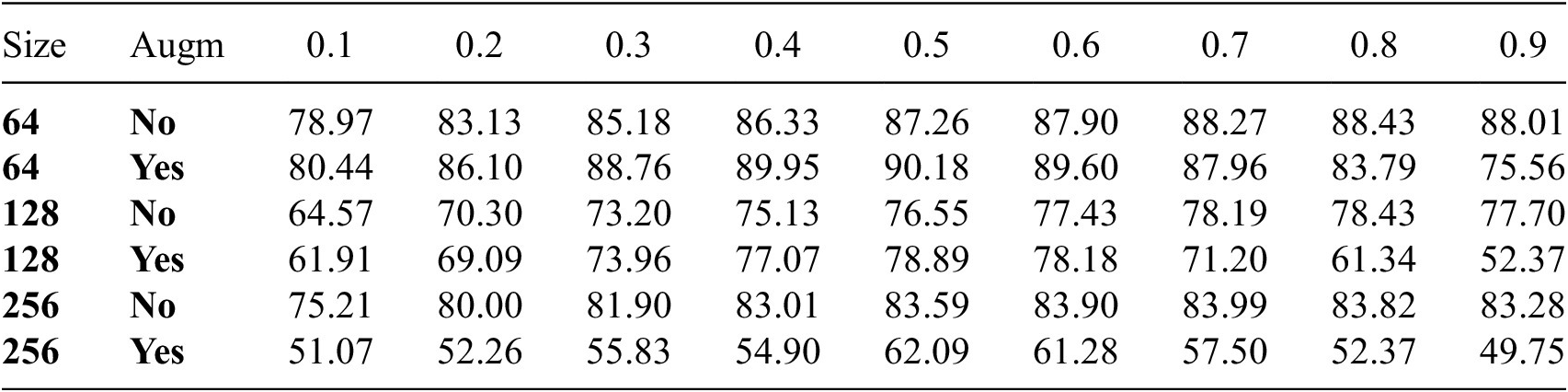
Table 4. Long description
The table consists of 11 columns and 7 rows. The first two columns are Size and Augm (Augmentation). The subsequent nine columns are numerical thresholds: 0.1, 0.2, 0.3, 0.4, 0.5, 0.6, 0.7, 0.8, and 0.9.
* Row 1: Size 64, Augm No. Accuracy values range from 78.97 at 0.1 to a peak of 88.43 at 0.8, ending at 88.01 at 0.9.
* Row 2: Size 64, Augm Yes. Accuracy values range from 80.44 at 0.1 to a peak of 90.18 at 0.5, then decreasing to 75.56 at 0.9.
* Row 3: Size 128, Augm No. Accuracy values range from 64.57 at 0.1 to a peak of 78.43 at 0.8, ending at 77.70 at 0.9.
* Row 4: Size 128, Augm Yes. Accuracy values range from 61.91 at 0.1 to a peak of 78.89 at 0.5, then decreasing sharply to 52.37 at 0.9.
* Row 5: Size 256, Augm No. Accuracy values range from 75.21 at 0.1 to a peak of 83.99 at 0.7, ending at 83.28 at 0.9.
* Row 6: Size 256, Augm Yes. Accuracy values are lower, starting at 51.07 at 0.1, peaking at 62.09 at 0.5, and ending at 49.75 at 0.9.
F1 Score of DOC-CrackNet for all the tested patch sizes and with or without augmentation
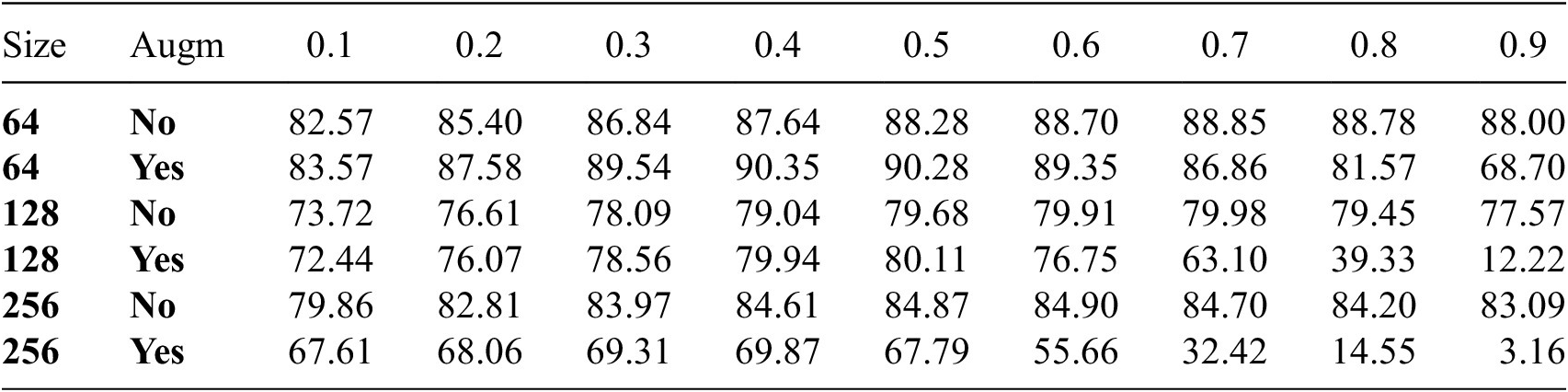
Table 5. Long description
The table consists of 11 columns. The first two columns are Size (64, 128, 256) and Augm (No or Yes). The subsequent nine columns are numerical thresholds from 0.1 to 0.9.
* Size 64, Augm No: Scores range from 82.57 at 0.1 to a peak of 88.85 at 0.7, ending at 88.00 at 0.9.
* Size 64, Augm Yes: Scores range from 83.57 at 0.1 to a peak of 90.35 at 0.4, then decreasing to 68.70 at 0.9.
* Size 128, Augm No: Scores range from 73.72 at 0.1 to a peak of 79.98 at 0.7, ending at 77.57 at 0.9.
* Size 128, Augm Yes: Scores range from 72.44 at 0.1 to a peak of 80.11 at 0.5, then dropping sharply to 12.22 at 0.9.
* Size 256, Augm No: Scores range from 79.86 at 0.1 to a peak of 84.90 at 0.6, ending at 83.09 at 0.9.
* Size 256, Augm Yes: Scores range from 67.61 at 0.1 to a peak of 69.87 at 0.4, then dropping significantly to 3.16 at 0.9.
According to the results in Tables 4 and 5, the architecture that significantly outperformed the others was DOC-CrackNet trained on 64×64 patches with data augmentation. If an optimal
$ \sigma =0.5 $
 was selected, this model achieved an accuracy of 90.18% and an F1-score of 90.28% . This performance discrepancy is directly related to the receptive field provided by each patch dimension. Because DOC-CrackNet classifies the central pixel based on the surrounding window, the 64×64 patch provides sufficient local morphological context to recognize the linear continuity of a crack without overwhelming the network with distant background texture. Conversely, the larger
$ 128\times 128 $
was selected, this model achieved an accuracy of 90.18% and an F1-score of 90.28% . This performance discrepancy is directly related to the receptive field provided by each patch dimension. Because DOC-CrackNet classifies the central pixel based on the surrounding window, the 64×64 patch provides sufficient local morphological context to recognize the linear continuity of a crack without overwhelming the network with distant background texture. Conversely, the larger
$ 128\times 128 $
 and 256×256 patches introduce excessive global noise and severe class imbalance (i.e., a vastly higher ratio of background concrete pixels to thin crack pixels). This negatively impacts the classification of the central pixel, particularly when spatial augmentations are applied. Therefore, the 64×64 patch size with data augmentation and a threshold of
$ \sigma =0.5 $
and 256×256 patches introduce excessive global noise and severe class imbalance (i.e., a vastly higher ratio of background concrete pixels to thin crack pixels). This negatively impacts the classification of the central pixel, particularly when spatial augmentations are applied. Therefore, the 64×64 patch size with data augmentation and a threshold of
$ \sigma =0.5 $
 was selected as the optimal baseline for the integrated framework.
4.3. Orientation estimation
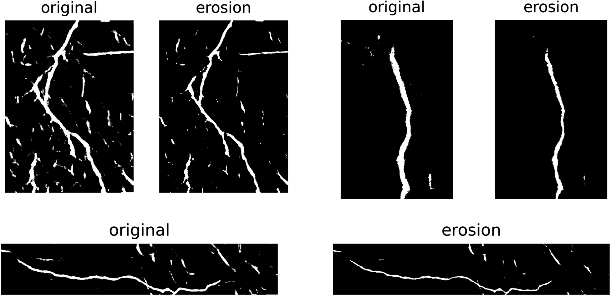
Once cracks were fully characterized, the procedure described in Section 3.6 was applied to the extracted patches for identifying their predominant direction. To this end, the effects of the erosion filter on three different masks are shown in Figure 6.
Application of the erosion filter on three different masks. The general effect of applying the filter on the eroded masks caused an overall reduction of the noisy outliers.
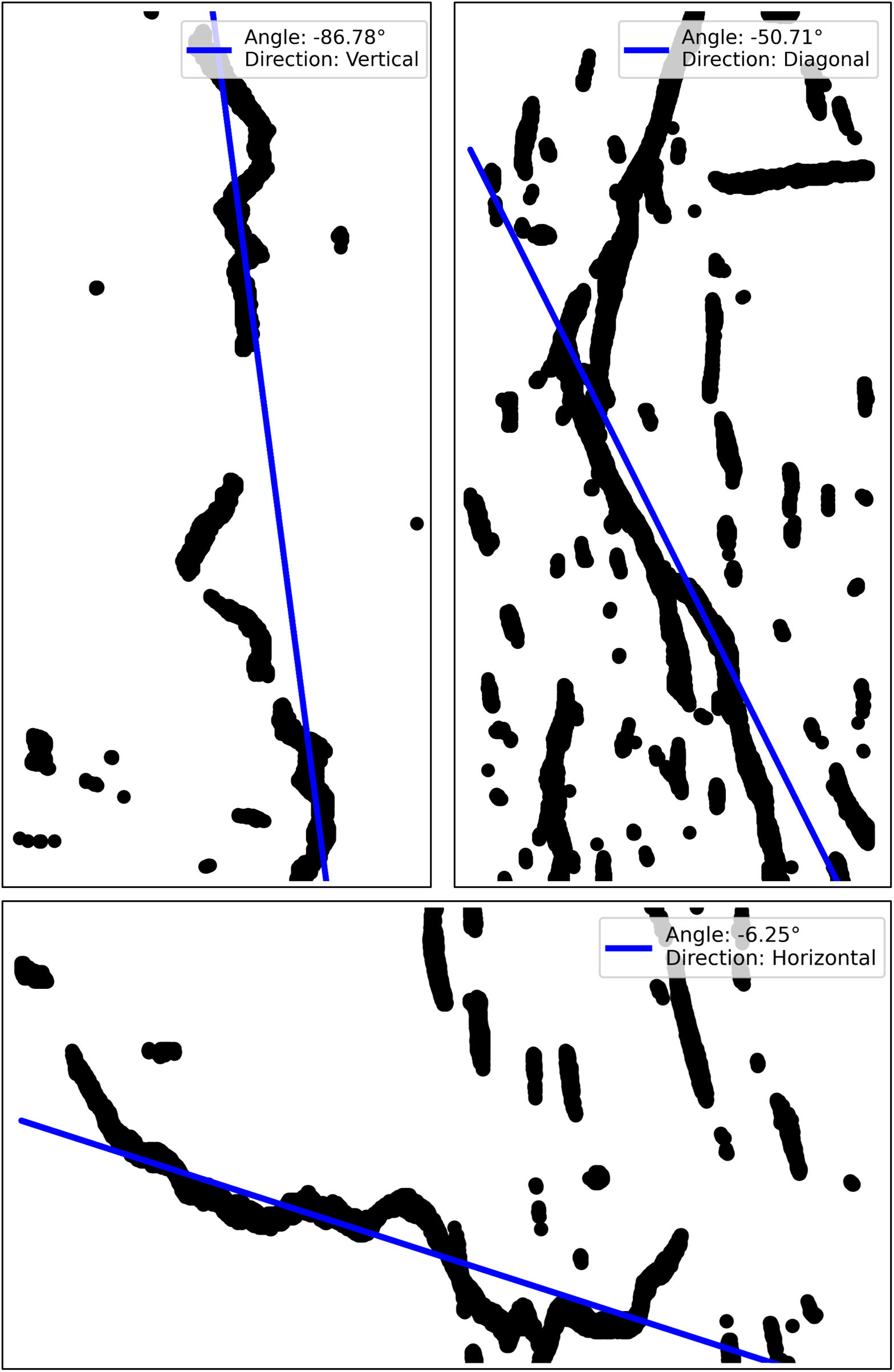
Subsequently, Figure 7 reports the results in terms of orientation, showing a blue line indicating the inclination and a legend reporting the angle and the desired output (i.e., vertical, diagonal, and horizontal).
The results of the orientation evaluation on the same masks are shown in Figure 6. As shown, the methodology could correctly evaluate the orientation of the crack in all three cases.
4.4. Qualitative evaluation and discussion
As the last step in assessing the effectiveness of DOC-Crack, an experimental evaluation is provided by performing a qualitative evaluation of the results achieved by DOC-CrackNet-129 on a set of images that do not belong to the training set. The images shown in Figure 8 were selected to highlight some of the main pros and cons of DOC-Crack by showing different situations. Specifically, Figure 8(a) shows the results that can be achieved when a single and visible crack is present in the image. In this case, DOC-CrackNet-129 provided robust and consistent results, despite the varying angles of the crack depicted in the patch. The same conclusions could be drawn by looking at Figure 8(c), where the network was able to identify an irregular and discontinuous crack with high reliability. However, it is worth noting that the network can be misled under specific circumstances due to certain occurrences in the provided patch. For example, Figure 8(b) shows some irregularities due to the formwork of the structural element, which in the patch appeared visually similar to vertical cracks. Analogously, Figure 8(d) presents several irregularities in the form of honeycombs and abrasions on the concrete surface, which could also be misinterpreted if the network is not provided with contextual information. These effects resulted in visual incoherence of the provided patches, as highlighted by the predictions provided by the network for both patches in Figure 8(b) and (d). In such cases, while the network is still able to properly track the main crack in both situations, the prediction was affected by a certain degree of noise. Future evolution of the algorithm should address these situations by adopting specific solutions, such as data preprocessing to filter out noisy backgrounds, fusion with 3D surface data to identify defects such as honeycombs, or semantic enrichment via knowledge embedded into large language models to provide contextual information and, therefore, filter out formwork effects on the structural elements.
Qualitative analysis. Each labeled subfigure represents a different crack in the dataset (on the left), with the associated crack identified by CrackNet (on the right).
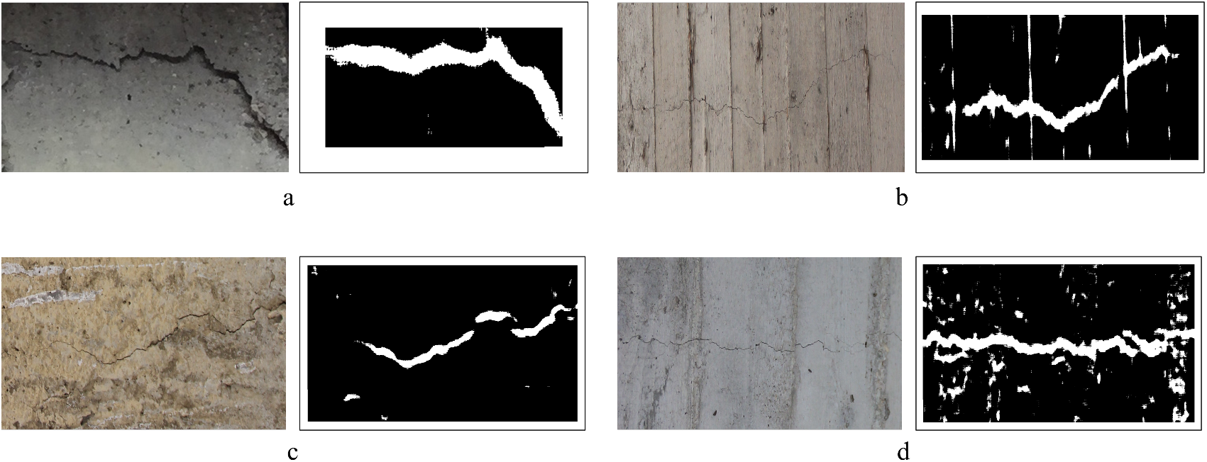
Figure 8. Long description
The figure contains four labeled sections, a through d, arranged in a two-by-two grid. Each section displays a side-by-side comparison of a grayscale or color photograph of a surface crack and a black-and-white binary mask representing the detected crack area.
* Panel a: Top-left. The photograph shows a wide, jagged horizontal crack in a dark gray concrete surface. The binary mask shows a thick, continuous white jagged line against a black background, accurately tracing the main crack path.
* Panel b: Top-right. The photograph shows a thin, faint crack on a light-colored wooden or textured concrete surface with vertical grain lines. The binary mask captures the main horizontal crack as a white line but also includes several vertical white streaks corresponding to the surface texture noise.
0* Panel c: Bottom-left. The photograph shows a fine, branching crack on a rough, tan-colored masonry surface. The binary mask shows a segmented white path that is thinner and more broken than in panel a, reflecting the finer nature of the crack.
* Panel d: Bottom-right. The photograph shows a very thin, horizontal crack on a light gray, weathered surface. The binary mask shows a central white horizontal path surrounded by significant white speckle noise, indicating a high level of surface interference in the detection process.
5. Application of DOC-Crack on a real case study
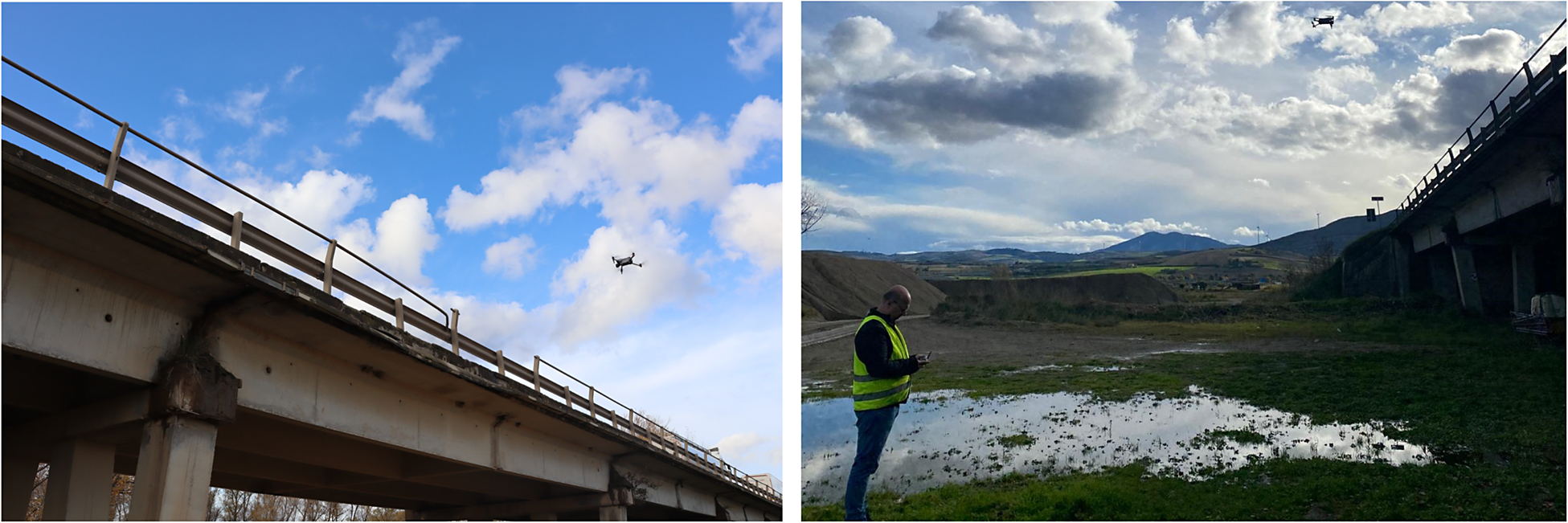
With the aim of testing the proposed procedure on a case study, DOC-Crack was used to investigate cracks on the deck of a real-life bridge. It is worth anticipating that, for privacy reasons, no registry information can be provided about the case study. The RC bridge is composed of frame piers and a deck characterized by three main beams. The focus of the investigation was oriented on the external beams, for which a survey through UAV was performed. In particular, a DJI Air 3 Fly More Combo, equipped with a 48MP camera, was used to take high-resolution images of the bridge. According to the procedure in Section 3.1, consecutive shots were performed (every 3 seconds) at a distance of around 1 meter, to completely survey different external beams, by ensuring a minimum overlapping zone 30%for the images. In Figure 9, the phase of the survey is reported.
Photos of the survey phase, performed through UAV flight.
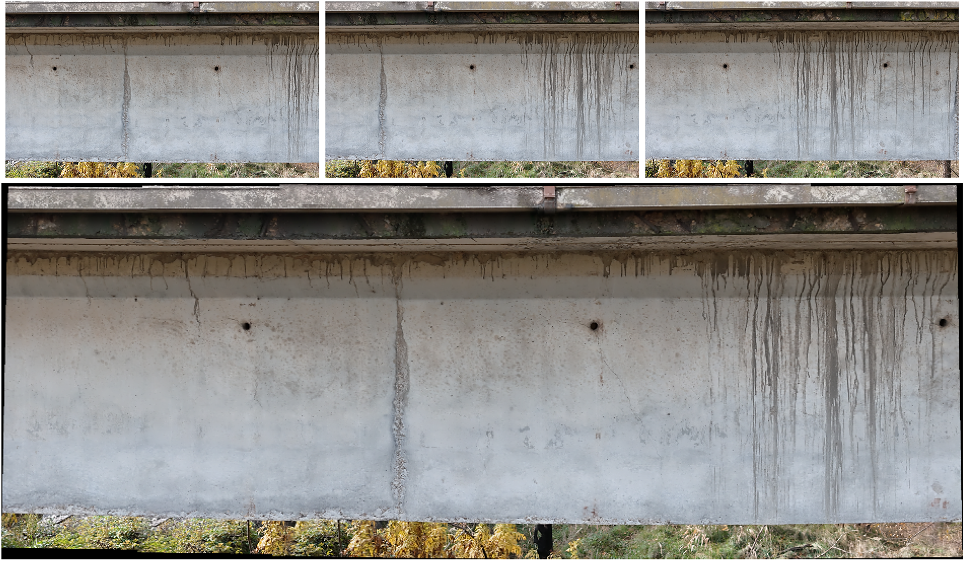
Once the data were collected, the proposed procedure consisted of preparing images for the stitching phase. For the case at hand, three consecutive images were selected for two different bays (named in the following, Case 1 and Case 2). Obviously, more than three photos could be included in the analysis, but the authors’ choice was aimed at reducing the computational effort in the image processing and to test DOC-Crack for more than one case (i.e., Case 1 and Case 2). Figures 10 and 11 show the three selected images and the related stitched image for Case 1 and Case 2, respectively, according to the approach reported in Section 3.2. It is worth observing that the stitching operation was performed by using as key points the holes in the beams (available for initial assembly of the bridge) and, as expected, the result was not affected by any distortion.
Case 1: A set of three consecutive shots and a stitched image.
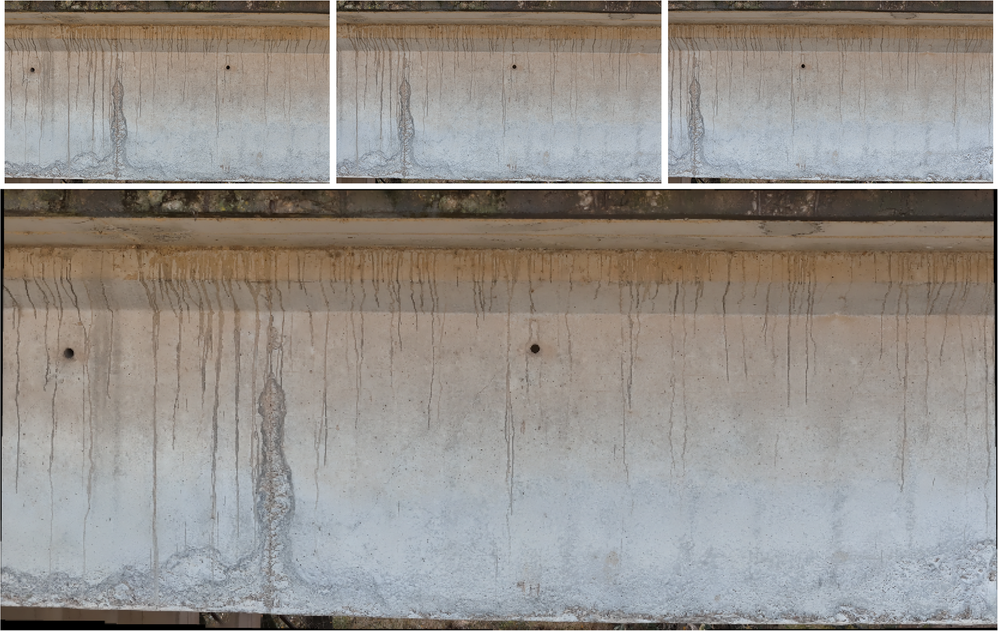
Figure 10. Long description
The top row contains three smaller, rectangular photos arranged horizontally. Each photo captures a segment of a weathered concrete girder with vertical water staining and small circular drainage holes. The first photo on the left shows two holes and heavy staining. The middle photo overlaps with the first, showing the second hole and a third hole. The third photo on the right overlaps with the middle, showing the third hole and the rightmost section of the girder.
The bottom panel is a large, wide-format photo that seamlessly combines the three top images into a single continuous view. This stitched image shows the full horizontal extent of the girder section, featuring three distinct circular holes spaced evenly. Numerous dark, vertical streaks from water runoff extend from the top edge down the face of the concrete. The bottom edge of the girder shows signs of efflorescence and surface degradation with a rougher, lighter-colored texture.
Case 2: A set of three consecutive shots and a stitched image.
The next step of the procedure consisted of crack detection on the stitched images. To this scope, as reported in Section 3.4, the trained version of YOLO11 was used, and the results can be observed for both Case 1 and Case 2 in Figure 12. From the analysis of the results, some aspects can be highlighted. First, as the primary objective of the proposed approach, the algorithm identifies almost all cracks, covering the effective crack pattern in the stitched image. After each bounding box provides a confidence score (a number close to the bounding box), which indicates the reliability of the prediction. In fact, for very thin cracks, albeit with a low confidence score, the algorithm is able to identify the considered defect, often also difficult to recognize by the human eye. Finally, as the main advantage of the trained algorithm, the proposed detector is able to distinguish the cracks from other parts of the images, such as the release agent used at the time of construction (i.e., the near-vertical darker lines in the figures), to confirm the goodness of the prediction (differently from the formwork lines in Figure 8). As a main disadvantage, the detector tends to subdivide long cracks into shorter ones, in accordance with the performed training. If from one hand, this can represent an issue for the proposed approach (especially for the counting), on the other hand, the cases in which some cracks are missed by the detector can be easily recognized by the user.
Crack detection on Case 1 and Case 2, respectively.
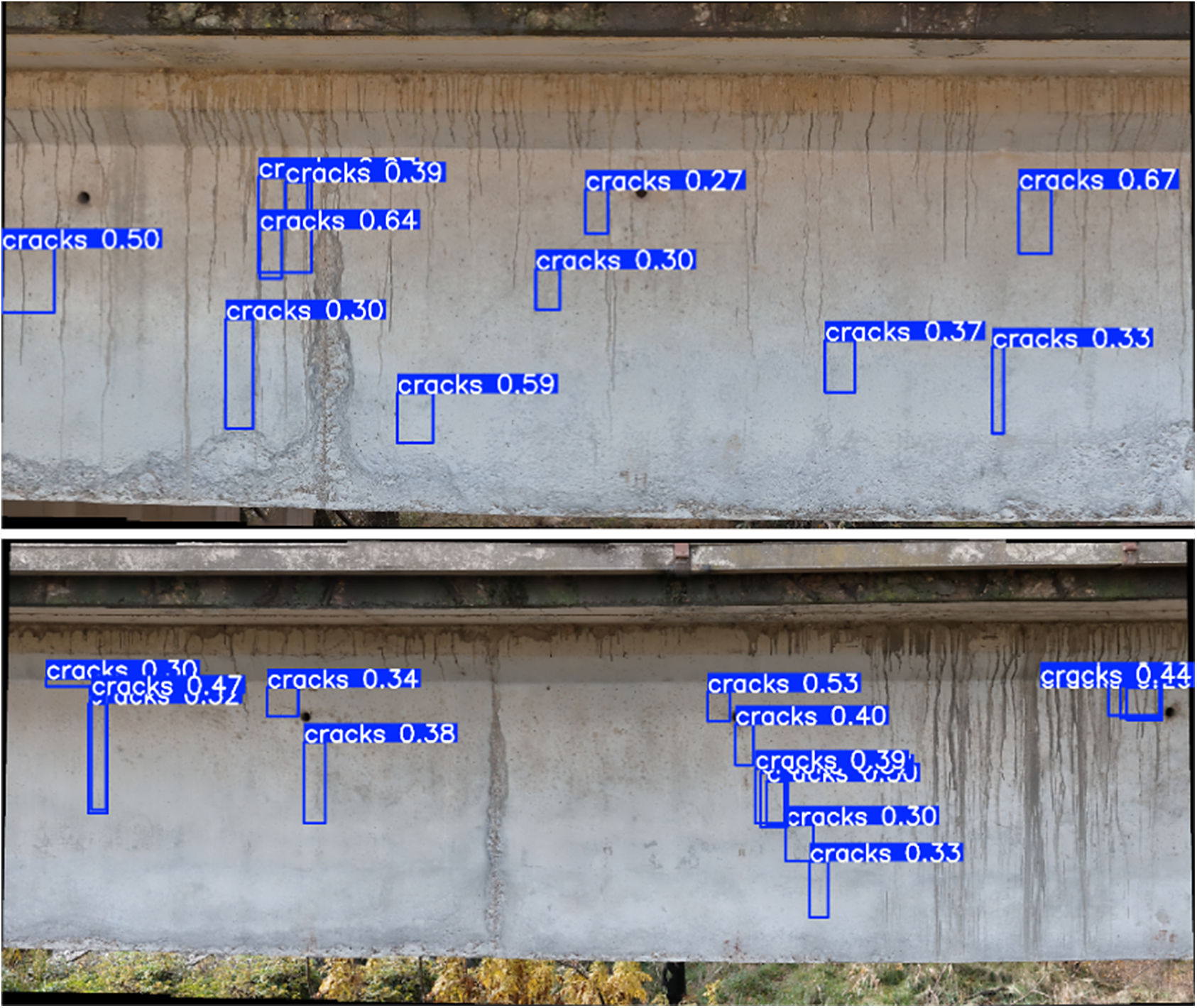
Figure 12. Long description
The top panel shows a weathered concrete beam with vertical water stains. Ten blue bounding boxes are distributed across the surface. From left to right, the labels and scores are: cracks 0.50, cracks 0.39, cracks 0.64, cracks 0.30, cracks 0.59, cracks 0.27, cracks 0.30, cracks 0.37, cracks 0.67, and cracks 0.33.
The bottom panel shows a similar section of the concrete beam with eleven blue bounding boxes. From left to right, the labels and scores are: cracks 0.30, cracks 0.47, cracks 0.32, cracks 0.34, cracks 0.38, a cluster of five overlapping boxes with scores 0.53, 0.40, 0.39, 0.30, and 0.33, and a final box on the far right labeled cracks 0.44.
After performing crack detection in the stitched image, the algorithm of crack segmentation, DOC-CrackNet, was applied. In particular, the model with higher performance, DOC-CrackNet-129 (defined in Section 4.1), was used for all detected cracks, and some results can be observed in Figure 13. In this latter, referring to six cases randomly chosen, the first row reports the cracks previously detected in the stitched image, while the second row reports the obtained estimation masks, assuming
$ \sigma $
 equal to 0.5. It is worth noting that the results in terms of estimation masks are reported as already elaborated with the erosion filter, in order to estimate the orientation (see later). Still, the third row highlights with a green patch the detected cracks, for the purpose of crack pattern definition to be reported on the original stitched image. The obtained results show a certain flexibility of DOC-CrackNet-129, which is able to detect different types of cracks, characterized by different thicknesses. In addition, a few noise effects can be observed to confirm the limitation mentioned in Section 4.4.
Results of DOC-CrackNet.
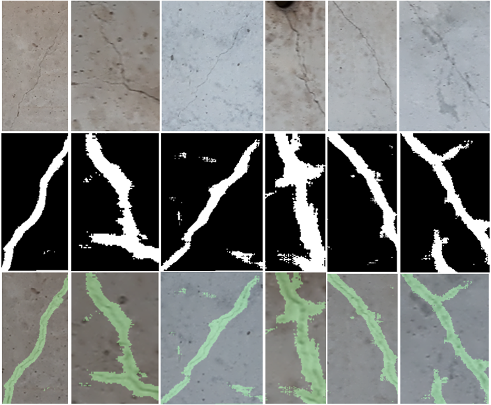
Figure 13. Long description
The grid consists of three distinct rows, each containing six vertical rectangular panels.
* The top row displays raw photographs of concrete surfaces. Each panel shows a different texture and color of concrete, ranging from tan to light gray, with thin, dark, irregular cracks running vertically or diagonally across the surface.
* The middle row shows binary segmentation masks corresponding to the panels above. These are high-contrast black and white images where the detected cracks are represented as thick, jagged white lines against a solid black background. The white lines vary in thickness and branching patterns, mirroring the geometry of the cracks in the top row.
* The bottom row displays the final D O C dash Crack Net results. These panels show the original concrete photographs from the top row with a semi-transparent green overlay applied precisely over the detected crack areas. The green highlights follow the exact path of the cracks, demonstrating the model’s localization accuracy across different surface conditions.
Finally, the last step of the proposed procedure consists of defining the cracks’ orientation. According to Section 4.3, the proposed algorithm was used, and the obtained results are reported in Figure 14. Using the ranges defined in Table 2, the evaluation of the inclination degree is reported. Figure 14 shows, on the same set of cracks reported in Figure 13, that three cracks were classified as vertical and three were classified as diagonal.
Results in terms of orientation.
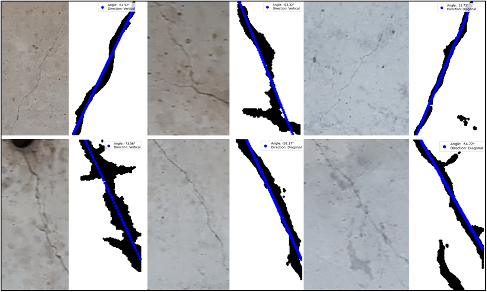
Figure 14. Long description
The multi-panel layout consists of two rows and three columns of image pairs. Each pair shows a close-up photo of a crack in a concrete surface next to a black-and-white binary mask where the crack is represented in black. A blue line is superimposed on the black mask to indicate the calculated orientation. Each mask includes a legend in the top right corner.
Top Row
* Left Pair: Angle 61.92 degrees, Direction Vertical. The crack runs diagonally from bottom-left to top-right.
* Middle Pair: Angle minus 63.32 degrees, Direction Vertical. The crack runs from top-left to bottom-right with a horizontal branch at the bottom.
* Right Pair: Angle 53.73 degrees, Direction Diagonal. The crack runs steeply from bottom-left to top-right.
Bottom Row
* Left Pair: Angle minus 73.56 degrees, Direction Vertical. The crack runs from top-left to bottom-right with several jagged horizontal protrusions.
* Middle Pair: Angle minus 58.37 degrees, Direction Diagonal. The crack is a relatively straight line running from top-left to bottom-right.
* Right Pair: Angle minus 54.72 degrees, Direction Diagonal. The crack runs from top-left to bottom-right with a distinct fork near the top and a separate segment at the bottom.
In the end, the outcome of DOC-Crack is the crack pattern, which is shown in Figure 15. The obtained results suggest the importance of tools like DOC-Crack, which provides valuable information to users (e.g., surveyors of road management companies), and suggests possible interventions in view of risk mitigation.
Results of DOC-Crack on Case 1 and Case 2, respectively, showing crack patterns.
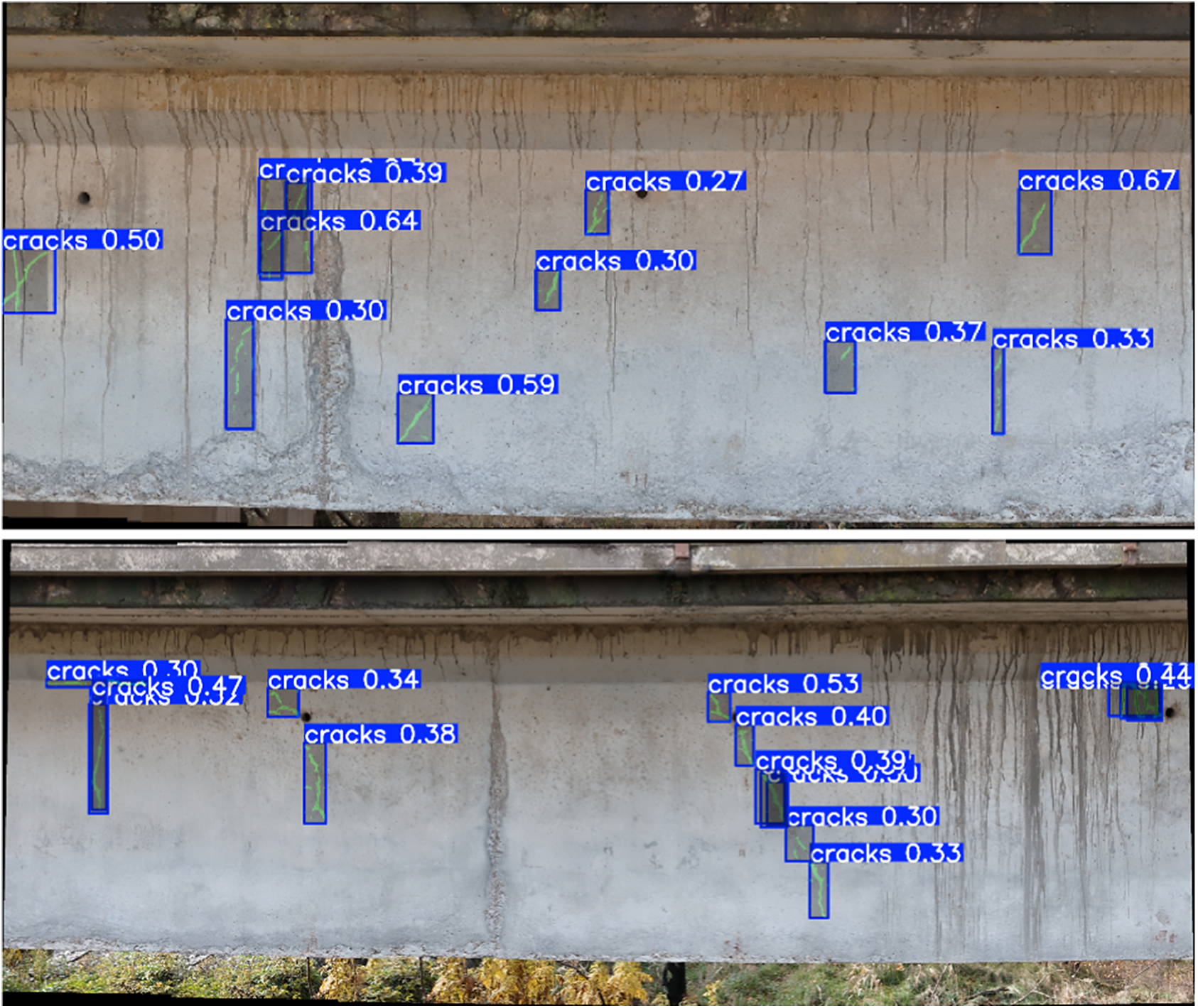
Figure 15. Long description
The two panels show a weathered concrete beam with vertical water staining and surface cracks.
In the top panel (Case 1), ten blue bounding boxes identify cracks with the following labels from left to right:
* cracks 0.50 on the far left.
* A cluster of three boxes labeled cracks 0.39, cracks 0.64, and cracks 0.30.
* cracks 0.59 located lower in the center-left.
* cracks 0.27 and cracks 0.30 in the center.
* cracks 0.37 and cracks 0.33 on the right.
* cracks 0.67 on the far right.
In the bottom panel (Case 2), nine blue bounding boxes identify cracks from left to right:
* A cluster on the left with cracks 0.30, cracks 0.47, and cracks 0.32.
* Two boxes in the center-left labeled cracks 0.34 and cracks 0.38.
* A vertical staggered cluster in the center-right labeled cracks 0.53, cracks 0.40, cracks 0.39, cracks 0.30, and cracks 0.33.
* A cluster on the far right labeled cracks 0.44 and cracks 0.29.
Each box contains a green line tracing the specific path of the detected crack within the concrete surface.
6. Discussion
6.1. Manual versus automatic crack identification
As the final step of the work, it is interesting to assess the results of DOC-Crack against manual crack annotation. To this end, one of the two cases studied was selected, namely the stitched image of Case 1 (Figure 10). In this case, the authors—acting as domain experts in structural engineering—manually identified visible cracks using red traces, as shown in Figure 16. Comparing the capacity of the human eye against the output of DOC-Crack (see Figure 15) highlights several key aspects.
Case 1: Results of manual annotation.
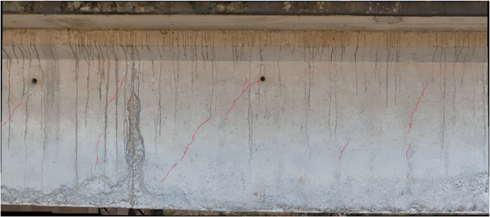
Regarding crack detection, as previously noted, DOC-Crack tends to subdivide long, continuous cracks into shorter segments whenever visual discontinuities (e.g., surface noise or patch borders) occur. Conversely, the human eye inherently extrapolates the entire crack development across the surface of the element. This discrepancy leads to different final counts: the automated detection identified 11 short cracks, while manual detection identified nine continuous cracks (plus one branching off in the central part). While simple heuristic postprocessing rules, such as merging adjacent detections based on distance proximity and orientation continuity, can partially mitigate this over-counting, they often fail or introduce false connections in dense, highly branched spider-web crack patterns. Therefore, this counting artifact is acknowledged as a current limitation of the pixel-level segmentation approach. Future developments will investigate transitioning to true instance-level segmentation to organically map complex, multibranching cracks as unified instances without manual parameter tuning.
As for crack orientation, according to the geometric rules established for the automated computation, both the manual and automatic approaches returned consistent results for the main crack branches.
6.2. Limitations
It is important to underline that the proposal uses standard feature-based homography to generate the composite panoramas of the RC bridge. However, the overall reliability of the proposed framework is based on specific operational assumptions during image acquisition. Specifically, the camera should maintain a roughly perpendicular optical axis to the surface, and there should be a high degree of overlap between consecutive frames. Furthermore, as the homography mathematically assumes that the target surface is a bidimensional planar element, it may become insufficient when inspecting nonplanar elements, such as cylindrical piles, introducing local distortions or misalignments during stitching. These artifacts are particularly detrimental, as they can visually fracture continuous crack patterns into disjunct segments, thereby artificially inflating the automated crack count and distorting the orientation mapping. To overcome these limitations, future work could replace the bidimensional stitching module with 3D photogrammetry to be applied before the detection pipeline.
Furthermore, it is important to underline how assigning a single, dominant orientation via linear fitting is an inherent limitation when dealing with irregularly branched cracks. Hence, while the proposal fitting proved reliable for the relatively straight crack patterns in the current case study, representing a complex, multidirectional crack as a single linear vector oversimplifies its local geometry. Future iterations of the framework will explore instance-level skeletonization to map varying orientations along the continuous path of a single curved crack.
Finally, it is important to note that the framework may exhibit partially overlapping cracks or cracks that are partially split into multiple segments. To this end, several approaches can be integrated into future works. For example, the nonmaximum suppression step of a YOLO-based algorithm can be enhanced to consider proximity constraints, therefore merging multiple nonoverlapping bounding boxes. This would allow us to maintain proper performance while avoiding instance segmentation techniques, which may entail a higher computational cost.
7. Conclusions
The paper presents an automated framework for characterizing crack patterns in RC bridges. The proposed tool, named DOC-Crack, is capable of detecting, counting, and orienting cracks in structural elements. The pipeline consists of various stages. The first step involves data collection, where a stack of photos for a structural element to inspect is collected, ensuring an overlap between consecutive images. In the second step, a phase of image stitching is proposed, which enables the acquisition of an image encompassing the near-full structural element to be investigated. The third step aims to elaborate a pipeline of DL algorithms, including an improved object detector specifically trained on a dataset of cracks, and a pixel-based segmentation algorithm to identify cracks on the output of the detection. Based on the elaborations performed, DOC-Crack enables the counting of cracks and the definition of their related orientation. The output of DOC-Crack is the crack pattern of the inspected structural element, which can serve as support for domain experts in assessing the current state of the structure and predicting possible future issues, as well as planning related interventions.
As shown throughout the manuscript, various advantages can be mentioned regarding DOC-Crack. Specifically, the proposed image stitching enables the reconstruction of the overall appearance of the RC element by exploiting invariant local features, thereby providing a comprehensive perspective of the element under investigation. Afterwards, the segmentation algorithm led to a per-crack evaluation, providing the effective trace and orientation of each visible crack. Overall, DOC-Crack offers several advantages, including its modularity, which allows each step to be independently deployed and used as needed. In addition, the proposed approach offers an aseptic visual information of cracks on the element to domain experts. The real aim of the authors is to provide an output that must be examined by the structural engineer, who can perform the necessary evaluations and make decisions. As a main disadvantage, while the network is able to identify and track the main cracks in the figures, some predictions can be affected by noise, which can result in an inaccurate final crack pattern. Still, although almost all cracks are detected, long cracks could be subdivided into smaller ones, biasing the final count but not affecting the crack pattern. Future evolutions of the algorithm should address these situations by adopting specific solutions, such as data preprocessing to filter out noisy backgrounds, fusion with 3D surface data to identify defects such as honeycombs, semantic enrichment via knowledge embedded into large language models to provide contextual information, and, therefore, filter out formwork effects on the structural elements. In addition, future developments should leverage the intrinsic parallelizability of the proposed pipeline, which, with an optimized implementation, could provide real-time capabilities on constrained hardware, such as low-end system-on-a-chip or smartphones.
Data availability statement
The data supporting the findings are available at https://doi.org/10.5281/zenodo.18218986 Cardellicchio et al. (Reference Cardellicchio, Ruggieri, Nettis, Renò, Di Mucci and Uva2026). The other datasets can be found in the referenced publications.
Acknowledgements
All authors thank Prof. Angelo Doglioni for the UAV survey.
Author contribution
Conceptualization: A.C., V.R., S.R.; Data curation: A.C., V.R., V.M.D.M.; Data visualization: A.C., V.R.; Funding: G.U.; Methodology: A.C., V.R., V.M.D.M.; Review original draft: Ag.N., V.R., An.N., S.R., G.U.; Writing original draft: A.C, S.R. All authors approved the final submitted draft.
Funding statement
S.R. thanks funding by Fabre Consortium, within the research grant “Sviluppo e implementazione di strategie basate sulla Intelligenza Artificiale per l’analisi e il monitoraggio del rischio strutturale di ponti e viadotti esistenti.” An.N. and G.U. thank funding by Centro Nazionale Sustainable Mobility Center, within the framework of “MOST” project, CUP code: D93C22000410001.
Competing interests
The authors declare none.
Ethical standard
The research adheres to all ethical guidelines, including compliance with the legal requirements of the study country.
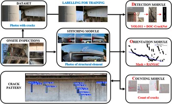
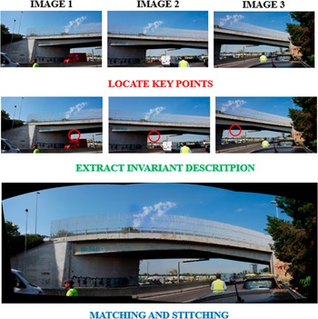

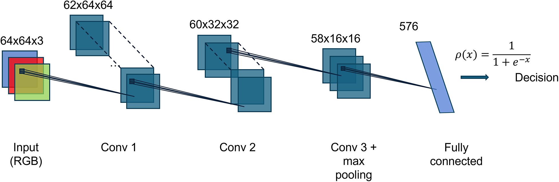


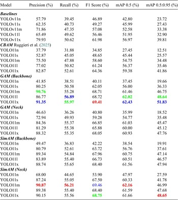
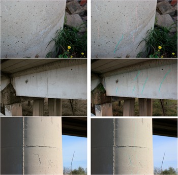
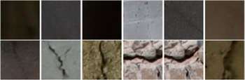
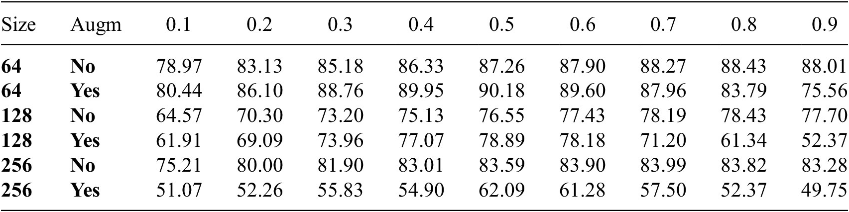
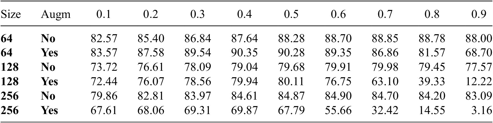
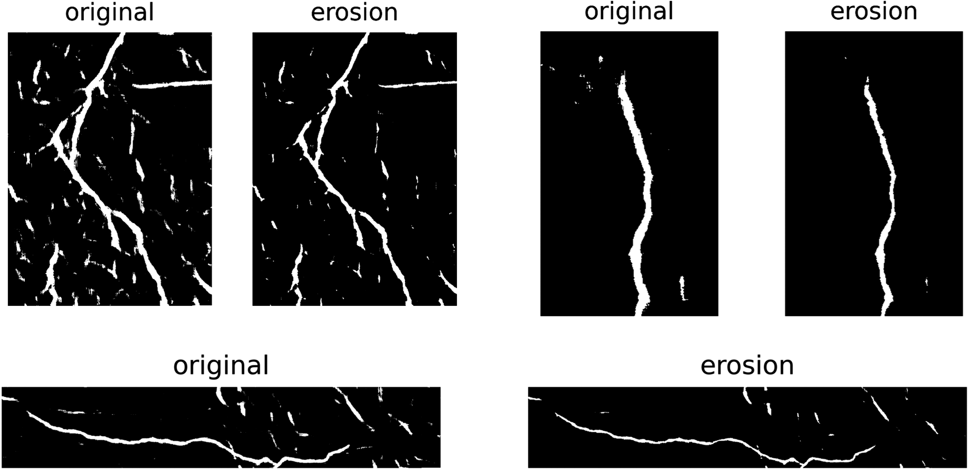
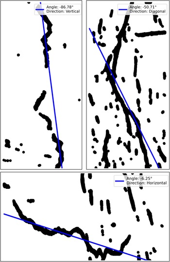
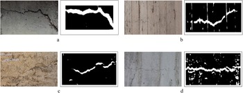
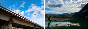
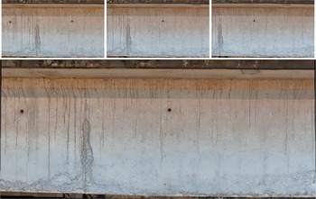
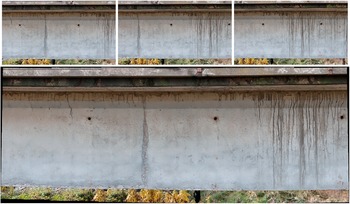
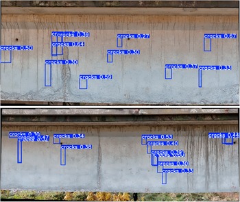
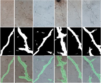
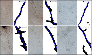
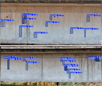
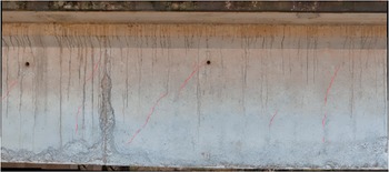

 Open access


Comments
No Comments have been published for this article.