


1. Introduction
Like many other countries, the US has experienced a resurgence in inflation in recent years, not seen in nearly 40 years. The initial rise in measured inflation can be partly attributed to the breakdown of the global supply chain following the COVID pandemic and the rise in energy prices, influenced by geopolitical disruptions such as the war in Ukraine and the countervailing sanctions on Russia’s export of oil and natural gas. However, the overtly expansionary monetary policy, through quantitative easing and the policy interest rate kept near the zero lower bound for a while, also bears some responsibility, especially for the increase in core (trend) inflation.
It has long been thought that the quantity of money in circulation has a direct bearing on an economy’s general price level (e.g., Fisher, Reference Fisher1911; Friedman, Reference Friedman and Friedman1956), implying that an increase in nominal money supply beyond a rise in real money demand leads to a higher price level, thus being a key determinant to core inflation. Yet, central banks’ emphasis on the short-term policy interest rate in the conduct of monetary policy, as well as its predominant use as a modelling tool by researchers and central banks, has relegated the importance of money in monetary policy to the background, possibly overlooking it by leaving it in a blind spot.
Empirically, following Bernanke and Mihov (Reference Bernanke and Mihov1998) and Christiano et al. (Reference Christiano, Eichenbaum, Evans, Christiano, Eichenbaum and Evans1999), a significant strand of the literature using structural vector autoregressive (VAR) models has found that shocks to the Fed Funds rate appeared to capture impulse response functions (IRFs) that are consistent with the expected economic intuition for their dynamic impact on interest rates, output, some narrow or somewhat broader money aggregates, and sometimes on inflation or the price level.Footnote 1 It became widely accepted that a central bank’s stance on monetary policy can be accurately represented, or extracted, from the policy interest rate, i.e., the Fed Funds rate for the US. However, the evidence was not entirely free from empirical puzzles regarding prices and output, which vary depending on the sample and variables in the model. In particular, the occurrence of a so-called price puzzle happens when what is identified as a restrictive monetary policy is followed by a counterintuitive empirical rise in prices.
When bringing up measures of money supply, the literature typically referred to conventional simple-sum aggregates, which impose that all components of an aggregate are perfectly substitutable. However, Barnett (Reference Barnett1980) effectively showed that, contrary to simple aggregates, the demand for Divisia money services has firm microfoundations that are consistent with welfare-maximizing households. Therefore, a more appropriate measure to represent the amount of medium of exchange in circulation, such as a Divisia index, could be relevant to assess its ability to better capture the state of monetary policy.
Recently, notable papers (such as Keating et al. Reference Keating, Kelly, Smith and Valcarcel2019, Belongia and Ireland, Reference Belongia and Ireland2019, Chen and Valcarcel, Reference Chen and Valcarcel2021, Reference Chen and Valcarcel2025) have found that Divisia money empirically matters, has informational content, but has been neglected in mainstream studies on the empirical role of money. Some papers have used time-invariant models, while others have used time-varying parameter (TVP) models.Footnote 2 In particular, Keating et al. (Reference Keating, Kelly, Smith and Valcarcel2019), using quarterly data up to 2015, and Chen and Valcarcel (Reference Chen and Valcarcel2021), using monthly data for the 1988–2020 period, find that, unlike Fed Funds rate-based shocks, structural monetary policy shocks estimated with Divisia measures of money do not exhibit a counterintuitive rise in the price level in response to restrictive monetary policy.
It might be argued that the Fed Funds rate’s inadequacy in representing monetary policy post-2008 is not surprising, given the Fed’s use of unconventional tools. Still, tracking the central bank’s instruments is different from understanding the overall stance of monetary policy, especially when considering its effects on output and prices.
One might question whether this result is robust and why it has remained barely known or acknowledged. The recent COVID episode, with its inflationary and disinflationary spells, offers a “natural experiment,” given the scale of the latest QE interventions, as inflation did not materialize in previous QE episodes following the 2007–2009 Great Financial Crisis.Footnote 3
Using samples of quarterly data from 1967Q1 to 2023Q4, this paper builds on earlier work. It takes advantage of recent episodes characterized by an important expansionary monetary policy from quantitative easing in response to the pandemic, followed by a rise in inflation, and then a renewed focus on getting inflation back around the 2% target. Combining new data with both traditional and new econometric tools, we assess the stability of the sign and size of key macroeconomic variables’ responses to monetary shocks throughout a period marked by many disturbances. Using block-recursive identifying restrictions, we apply two estimation methods to extract structural monetary policy shocks from alternative indicators.
Time-invariant structural VAR (SVAR) models are first used to revisit the typical identification restrictions (such as in Christiano et al. Reference Christiano, Eichenbaum, Evans, Christiano, Eichenbaum and Evans1999, Christiano et al. Reference Christiano, Trabandt, Walentin, Christiano, Trabandt and Walentin2010, and Keating et al. Reference Keating, Kelly, Smith and Valcarcel2019), comparing models that include either the Fed Funds rate, a Wu and Xia’s (Reference Wu and Xia2016) shadow rate with conventional or Divisia monetary aggregates.Footnote 4 Time-invariant impulse response functions (IRFs) for key macroeconomic variables are generated from these fixed-coefficient VARs, and their robustness is evaluated across different subsamples and variable sets.
We then use Goulet Coulombe’s (Reference Goulet Coulombe2025) 2-step ridge regression estimator to derive time-varying IRFs from TVP-VARs to assess whether these macroeconomic variables’ responses have been consistent throughout the years, notwithstanding the various developments in the US economy and in the conduct of monetary policy. This alternative estimator, recently developed, offers advantages that could be beneficial for addressing the empirical relevance of money. In particular, except for the estimation of one hyperparameter, in contrast to the Bayesian estimation of TVP models, it does not face the challenges of handling numerous hyperparameters and the requirement for an initial training sample that omits many observations.
Empirical evidence proves to be relevant for accurately capturing the dynamics of key macroeconomic variables since the late 1960s. Evaluating the forecasting ability and information content of Divisia measures confirms their usefulness and supports the superiority of models that include them for studying monetary policy transmission. Interest rates fail to produce dynamic responses free from empirical puzzles or consistent with expected intuition, for both earlier and extended sample periods past the early 2000s. When considering different subsamples, Divisia measures produce impulse response functions that better align with expected economic intuition and are less prone to empirical puzzles compared to interest rates or simple-sum aggregates, both in terms of size and duration of the impact. TVP-VAR evidence is particularly revealing and strongly supports our conclusion that the theoretically superior Divisia indices for monetary aggregates yield puzzle-free estimated IRFs for both output and prices throughout the 1967–2023 period. Furthermore, key macroeconomic variables are generally quicker to react to Divisia monetary policy shocks and the responses are often more important compared to alternative policy indicators.
Taking into account the latest inflation spell and using recent econometric developments, our results reinforce the idea that money, especially Divisia money, is important and has an explicit role in modelling and understanding monetary policy. Consequently, the long-held presumption in macroeconomics that the shocks to the central bank policy rate are the sole and central signal of monetary policy can be misleading or at least incomplete in characterizing the monetary policy stance and its impact, especially on prices.
The paper is structured as follows. Section 2 discusses how money has taken a back seat in monetary policy for more than three decades. Section 3 summarizes the concepts and the motivation for preferring Divisia monetary aggregates indices over traditional simple-sum monetary aggregates. Section 4 presents the econometric approach. Next, Section 5 presents and discusses the empirical results, while Section 6 provides concluding remarks and suggests possible extensions.
2. Monetary policy and inflation: money vs. the policy interest rate
Measured inflation (the percentage change in the price level between two periods) may involve both transitory and trend components. Supply shocks, such as a surge in energy prices or disruptions in the global supply chain, lead to a temporary increase in measured inflation. In the presence of nominal rigidities, the gradual adjustment of prices of some goods and services can be recorded in the overall price level over several quarters.Footnote 5
Assuming that all money in circulation is willingly held, the equilibrium between money supply and demand implies that the difference between the growth rates of the supply in the nominal quantity of money and the real demand for money must equate to the percentage change in the price level. This holds true despite nominal rigidities and the short-term non-neutrality of money, notwithstanding the operational modalities underlying the implementation of monetary policy.
Monetary policy implementation is a chain process, starting from a central bank’s use of tools to reach operating targets, which then impact intermediate targets or information indicator variables, ultimately achieving the monetary authority’s primary target, as illustrated in Figure 1.
Alternative monetary policy chains.
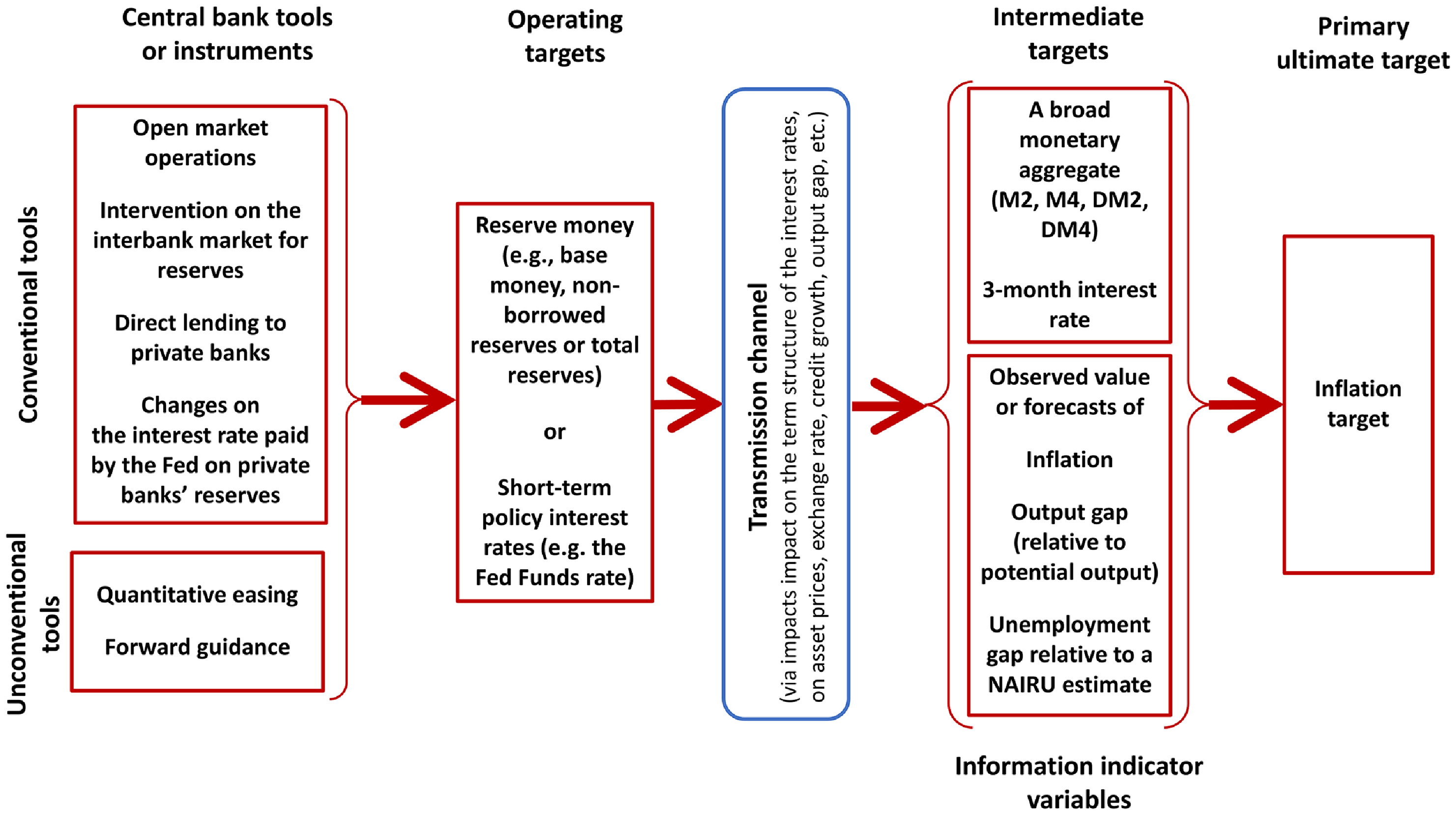
In the US, once the effects of the temporary non-neutrality of money have subsided, the Federal Reserve’s ultimate target can be thought of as a 2% value for core inflation. The central bank can use conventional tools like open market operations and interest rate adjustments, and unconventional tools like quantitative easing and/or forward guidance. The operating targets can be some reserve money or short-term interest rates, which impact various financial and economic variables, such as the term structure of the interest rates, asset prices, exchange rates, credit growth, output gap, etc. This leads to changes in intermediate targets (e.g., the 3-month or a higher maturity interest rate, or some measures of broad money) or information-indicator variables (e.g., the forecasts of some variables thought to be informative, such as future inflation, an output gap relative to potential output, or an unemployment gap relative to some value of a Non-Accelerating Inflation Rate of Unemployment), aiming at achieving the monetary policy goal.
In accordance with McCallum’s (Reference McCallum1989) graphic and schematic presentation, which we adapt in Figure 2, monetary policy can be understood, broadly speaking, in two alternative ways to achieve that the resulting growth path of some adequate and relevant monetary aggregate aligns with the inflation objective, for a given expected growth rate of real money demand and a given money multiplier.
A schematic representation of alternative intermediate targets for monetary policy: the monetary base versus the 3-month interest rate.
The dashed lines represent the “extreme” positions of the money demand and money supply curves due to the central bank’s imperfect controls of the intermediate target and the existence of uncertainty on either or both money demand and supply. Associated probability mass functions for the quantity of money and the short term interest rates respectively are represented below the horizontal axis and to the left axis of the graphs associated with the alternative targets. Under a short-term interest rate intermediate target, the position of the underlying money supply function is endogenously determined.
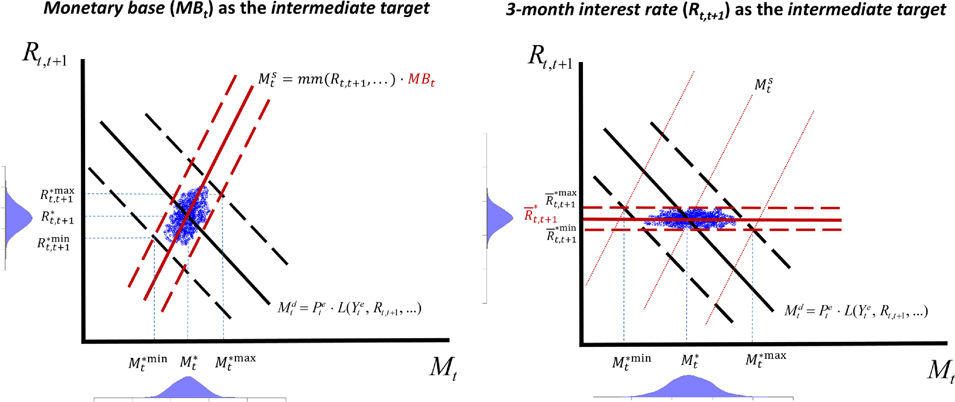
On one hand, if the operating target were considered to be the monetary base or a specific measure of private banks’ reserves, the central bank could chart its course so that the resulting path of broad money aligns with the inflation target. In particular, expected changes in either real money demand or the money multiplier would lead to adjustments in the operating target.
On the other hand, with the Fed Funds rate as the operating target, a central bank must adjust its very short-term one-day policy interest rate for a sufficient period to influence the specific higher-maturity nominal interest rate along the yield curve that enters the real money demand function. Thereby, monetary policy must be conducted in such a way that the resulting path of broad money growth aligns with the ultimate inflation target. Similarly, expected changes in real money demand, due to movements in the expected growth rate of real economic activity and the cost of financial intermediation, will also necessitate adjustments to the operating target.
However, empirical, theoretical, and central bank models have generally abstracted, for a long time, from the role of money supply in analyzing monetary policy. This de-emphasis is also evident in the conduct and discussion of monetary policy by central banks. Due to presumed instability in money demand and supply, central banks became disenchanted with using base money or broader money aggregates as instruments, intermediary targets, or indicators for monetary policy. This remained true even with the use of quantitative easing during the 2007–2009 Financial Crisis and the 2020 pandemic. For instance, while the Fed Funds rate was near zero, quantitative easing in the US led to massive expansions of the Federal Reserve’s balance sheet, with large purchases of either government or private bonds on the asset side and increases in financial intermediaries’ reserves and/or the US Treasury General Account on the liability side. Yet, monetary policy discussions continued to focus mainly on the policy rate.
Moreover, Taylor’s (Reference Taylor1993) and various extensions, e.g., Clarida et al. (Reference Clarida, Galí and Gertler2000), showed that monetary policy could be represented by an interest-rate rule or reaction function. This ties the evolution of the Fed Funds rate $_{ff}\bar {R}_{t}$
, to the quarterly average lagged value of the Fed Funds rate
$_{ff}\bar {R}_{t}$
, to the quarterly average lagged value of the Fed Funds rate $_{ff}{R}_{t-1}$
, the Wicksellian real natural rate
$_{ff}{R}_{t-1}$
, the Wicksellian real natural rate $ r^{N*}_t$
(also called the neutral real rate), the inflation gap relative to the inflation target
$ r^{N*}_t$
(also called the neutral real rate), the inflation gap relative to the inflation target $\pi ^\oplus$
, and a proxy for the output gap
$\pi ^\oplus$
, and a proxy for the output gap $\tilde {y}_{t}$
relative to potential real output.
$\tilde {y}_{t}$
relative to potential real output.
Hence, a generalized version of the Taylor rule describing the dynamics of the Fed Funds rate, $_{ff}\bar {R}_{t}$
, could be written as follows:
$_{ff}\bar {R}_{t}$
, could be written as follows:
 \begin{eqnarray} _{f\def\negativespace{}f}\bar {R}_{t} = \rho _m \, _{f\def\negativespace{}f}{R}_{t-1} + (1-\rho _m)\,\biggl [ r^{N*}_t + \pi _{t} + \phi _\pi \, \bigl (\pi _{t} - \pi ^\oplus \bigr) + \phi _{y} \, \tilde {y}_{t} \biggr] + \epsilon _t \,. \end{eqnarray}
The parameters of the monetary policy rule are interpreted as follows. The interest rate smoothing parameter $ 0\lt \rho _m\lt 1$
captures the central bank’s desire to avoid abrupt movements in the Fed Funds rate. The parameter
$ 0\lt \rho _m\lt 1$
captures the central bank’s desire to avoid abrupt movements in the Fed Funds rate. The parameter $\phi _\pi \gt 0$
indicates the central bank’s willingness to raise (lower) the policy rate when inflation exceeds (is less than) its target, adhering to the Taylor principle that it needs to move more than one-for-one with inflation. The output gap parameter
$\phi _\pi \gt 0$
indicates the central bank’s willingness to raise (lower) the policy rate when inflation exceeds (is less than) its target, adhering to the Taylor principle that it needs to move more than one-for-one with inflation. The output gap parameter $\phi _{y} \gt 0$
reflects the central bank’s intent to increase (decrease) the Fed Funds rate when real output exceeds (is below) trend output. Additionally, a non-systematic discretionary component
$\phi _{y} \gt 0$
reflects the central bank’s intent to increase (decrease) the Fed Funds rate when real output exceeds (is below) trend output. Additionally, a non-systematic discretionary component $\epsilon _t$
can be included to account for deviations from the systematic component due to other factors or changes in the usual weights given to inflation and output gaps, possibly in accordance with particular sensitivities expressed by the Federal Open Market Committee meetings’ participants.
$\epsilon _t$
can be included to account for deviations from the systematic component due to other factors or changes in the usual weights given to inflation and output gaps, possibly in accordance with particular sensitivities expressed by the Federal Open Market Committee meetings’ participants.
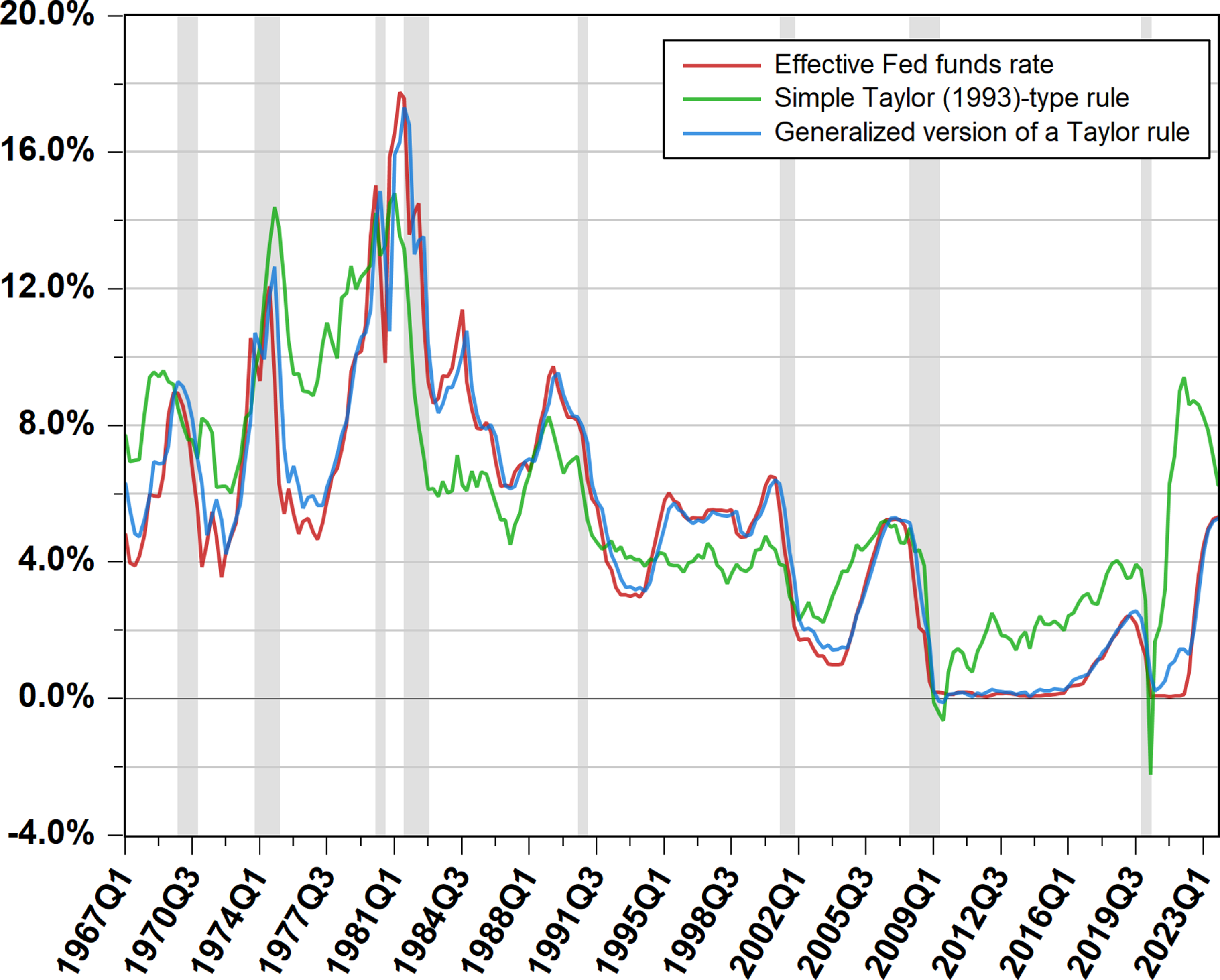
Using the Atlanta Fed’s Taylor Rule Utility with representative parameter values allows for the calibration of a generalized Taylor rule.Footnote 6 Figure 3 shows, almost astonishingly, that the resulting path of the ‘prescribed’ Fed Funds rate follows very closely the course of the observed Fed Funds rate from 1967Q1 to 2023Q4 (with a correlation of 0.974). Of course, no one would reasonably argue that the Federal Reserve was either pursuing a 2% inflation rate target in the late 1960s or in the 1970s, or that its sensitivity to inflation was necessarily as high as the one used in our simulation. Nonetheless, this suggests that tracking of the central bank’s generally preferred instrument may be a different thing than keeping track of the monetary policy stance.
Actual effective fed funds rate and Taylor rule’s prescriptions from 1967Q1 to 2023Q4.
The Taylor-rule prescribed values were generated using the Taylor Rule Utility made available by the Center for Quantitative Economic Research from the Federal Reserve Bank of Atlanta website (https://www.atlantafed.org/research/taylor-rule), with $r^{N*}_t=r^{N*} = 2\%$
, and a 2% inflation target,
$r^{N*}_t=r^{N*} = 2\%$
, and a 2% inflation target, $\phi _\pi = 0.5$
, and
$\phi _\pi = 0.5$
, and $\phi _{y} =0.5$
, for the Simple Taylor-type rule. For the generalized version, Laubach and Williams’s (Reference Laubach and Williams2003) time-varying 1-sided estimate of the natural real interest rate and an interest rate smoothing parameter
$\phi _{y} =0.5$
, for the Simple Taylor-type rule. For the generalized version, Laubach and Williams’s (Reference Laubach and Williams2003) time-varying 1-sided estimate of the natural real interest rate and an interest rate smoothing parameter $\rho _m = 0.85$
were used, while keeping a 2% inflation target,
$\rho _m = 0.85$
were used, while keeping a 2% inflation target, $\phi _\pi = 0.5$
, and
$\phi _\pi = 0.5$
, and $\phi _{y} =0.5$
.
$\phi _{y} =0.5$
.
Following Taylor’s (Reference Taylor1993) description of monetary policy by an interest-rate rule and its spin-offs, Woodford (Reference Woodford2003) then put forward some foundations suggesting that the policy interest rate may suffice to describe the monetary policy stance, while the quantity of money is adjusting endogenously.
In that vein, empirical literature, surveyed by Ramey (Reference Ramey and Ramey2016), used various econometric techniques to identify monetary policy shocks from movements in the Fed Funds rate. For example, Romer and Romer (Reference Romer and Romer1989, Reference Romer and Romer1994, Reference Romer and Romer1997) used archival Federal Reserve documents to pinpoint episodes of deliberate counter-inflationary policy decisions. Structural vector autoregressive models by Sims (Reference Sims1980, Reference Sims1986), Bernanke and Mihov (Reference Bernanke and Mihov1998), and Christiano et al. (Reference Christiano, Eichenbaum, Evans, Christiano, Eichenbaum and Evans1999, Reference Christiano, Trabandt, Walentin, Christiano, Trabandt and Walentin2010) estimate monetary policy shocks and their macroeconomic impacts by imposing identification restrictions. Additionally, high-frequency data studies, such as Nakamura and Steinsson (Reference Nakamura and Steinsson2018a, Reference Nakamura and Steinssonb), extract unexpected components of Fed Funds rate movements to measure exogenous monetary policy shocks.
The aforementioned empirical research and the central banks’ preference for the short-term policy interest rate as its instrument, along with Woodford’s (Reference Woodford2003) work, have made Taylor-type reaction functions prevalent in dynamic stochastic general equilibrium (DSGE) models to describe interest rate dynamics, typically excluding the quantity of money. In line with Woodford (Reference Woodford2003), it is assumed that there is no need to explicitly include a quantity of money variable, as the policy interest rate determines, in turn, the quantity of money along an implicit money demand curve, without explicitly modelling money demand and supply functions.
Accordingly, in typical New Keynesian DSGE models, monetary policy is captured by a Taylor-type rule, assuming no need for an explicit measure of the “quantity of money.” It is hypothesized that the nominal interest rate from the Taylor reaction function, up to a stochastic factor, will lead to an endogenous adjustment of an implicit “monetary aggregate” consistent with what is otherwise observed.
Consequently, a first issue pertains to whether abstracting from an explicit consideration of the role of money may have been misleading, at least to some extent, and even more so for some periods. The second issue we now turn to is the most appropriate concept of money.
3. On the theoretical and empirical relevance of Divisia monetary aggregates
3.1 Issues with traditional measures of money
The concept of a medium of exchange implies that its use as a generally accepted means of payment reduces the time, effort, and resources costs involved in trading goods and services. Undoubtedly, financial and goods-and-service innovations have transformed the form of “money” and its use over the last 40 years. Yet, notwithstanding what now constitutes the medium of exchange compared to what it was in the past, this does not change the idea that the general price level must also be compatible with an equilibrium in the market for money, with short-run nominal rigidities and long-run wage and price flexibility.
The theoretical foundation of core inflation being a monetary phenomenon stems from the equilibrium between money supply and demand, where economic agents freely hold the outstanding quantity of money. This equilibrium condition does not rely on some particular model of functioning of the labor market and/or the market for goods and services, holds regardless of the existence or not of nominal rigidities, and does not require the short-term and long-term money demands to be identical. Hence, trend inflation being driven by monetary considerations is not due to a Keynesian nature of the economy or a question pertaining to a school of thought.
Various issues have been invoked by central banks to turn away from the traditional monetary aggregates as guides to the conduct of monetary policy. In part, this was motivated by a somewhat vast empirical literature documenting the existence of instability in the demand for money aggregates, in the wake of Goldfeld (Reference Goldfeld1976) and the case for the missing money. Referring to traditional money aggregates, this instability has been mostly linked to instability in the short-term dynamics of money demand, and less so in the long-run money demand. Moreover, it appeared to be tied to post-1973 periods of significant financial innovations and changes in the components that can be counted as medium of exchange. For instance, Lucas and Nicolini (Reference Lucas and Nicolini2015) showed how the changes in the regulation of the banking sector in the 1980s had led to evidence of instability in the demand for M1, and they argued in favor of redefining “monetary aggregates by the functions they have in the payments system rather than by the institutions whose liabilities they are.” Furthermore, as discussed in Cukierman (Reference Cukierman and Cukierman2018), Noizet, Reference Noizet2018), and Ryan and Whelan (Reference Ryan and Whelan2023), the US conventional M2 money multiplier to the monetary base sharply fell, especially around 2008. This coincided with the financial crisis, which decreased the financial system’s readiness to lend in a more uncertain environment. Additionally, the nominal interest rate was near zero, and in October 2008, the US Federal Reserve Bank began paying interest on reserves held by financial institutions.Footnote 7
A non-trivial task is to link the theoretical concept of money to an empirical concept that is satisfactory and sufficiently broad, which Lucas (Reference Lucas1977) was alluding to in his own words:
“ in the ‘long run,’ general price movements arise primarily from changes in the quantity of money. Moreover, cyclical movements in money are large enough to be quantitatively interesting. [ $\ldots$
] The direct evidence on short-term correlations between money, output, and prices is much more difficult to read. [
$\ldots$
] The direct evidence on short-term correlations between money, output, and prices is much more difficult to read. [ $\ldots$
] In general, however, the link between money and these and other variables is agreed to be subject, in Friedman’s terms, to ‘long and variable lags.’ [
$\ldots$
] In general, however, the link between money and these and other variables is agreed to be subject, in Friedman’s terms, to ‘long and variable lags.’ [ $\ldots$
] These remarks do not, of course, explain why monetary effects work with long and variable lags. On this question little is known. It seems likely that the answer lies in the observation that a monetary expansion can occur in a variety of ways, depending on the way the money is ‘injected’ into the system, with different price response implications depending on which way is selected. This would suggest that one should describe the monetary ‘state’ of the economy as being determined by some unobservable monetary aggregate, loosely related to observed aggregates over short periods but closely related secularly.”
$\ldots$
] These remarks do not, of course, explain why monetary effects work with long and variable lags. On this question little is known. It seems likely that the answer lies in the observation that a monetary expansion can occur in a variety of ways, depending on the way the money is ‘injected’ into the system, with different price response implications depending on which way is selected. This would suggest that one should describe the monetary ‘state’ of the economy as being determined by some unobservable monetary aggregate, loosely related to observed aggregates over short periods but closely related secularly.”
This quote could thus be seen as an invitation to link the concept of money to a suitable and encompassing empirical counterpart.
3.2 The conceptual and theoretical case for Divisia measures of money
Typically, much of the literature has used conventional measures of monetary aggregates, defined as simple arithmetic sums of their components, to measure the medium-of-exchange volume in circulation. By construction, the reference to a traditional monetary aggregate implicitly assumes that all its components are perfectly substitutable, by implying that the services derived from holding and using each component are perfectly equivalent in providing the services of a medium of exchange. For instance, banknotes and demand deposits, whose holding yields a higher return, have the same unitary weight in the simple-sum aggregate. At the same time, traditional broader aggregates, such as M3 and M4, tend to overweight shadow bank services, while narrower aggregates exclude financial bonds from the financial markets on which companies finance themselves for maturities of less than one year. So, while a one-hundred-dollar bill and a one-hundred-dollar Treasury bill are considered perfect substitutes in a conventional broad monetary aggregate like M4, Treasury bills are surely less liquid. Besides, different monetary asset components may have a different impact on production, inflation, or other macroeconomic variables.
Furthermore, as shown by Barnett (Reference Barnett1980) and many subsequent contributions, a simple-sum monetary aggregate is incompatible with and internally inconsistent with microeconomic consumer demand theory. Therefore, the Barnett critique implies that a traditional monetary aggregate is unlikely to accurately measure the true flows of money services demanded by households.
Instead, William A. Barnett and various researchersFootnote 8 have proposed constructing and preferring the use of a Divisia index of monetary aggregation to measure the quantity of money.Footnote 9 Intuitively, the idea is to measure the flow of money services received in each period by households and firms from their holdings of monetary assets. In particular, in a calibrated New Keynesian DSGE model, Belongia and Ireland (Reference Belongia and Ireland2014) showed that, contrary to a theoretically flawed simple-sum aggregate, a Divisia monetary index is theoretically coherent for measuring monetary services and produces intuitively sensible impulse responses to various real and monetary shocks.
The Divisia measures are grounded in firm microfoundations aligned with households maximizing their welfare, making them theoretically superior to simple-sum aggregates for measuring the money supply. They take into account the varying levels of liquidity of different assets, and weight each component of the monetary aggregate by their degree of moneyness or their quality of money, represented by its user cost. Thus, the weight of each component varies inversely with their respective associated interest rates. For instance, nonbank money and demand deposits would have a higher liquidity value than term deposits.Footnote 10
3.3 The empirical case for Divisia measures of money
Simple-sum measures of money have also been known to be distorted on empirical grounds. Looking at evidence for seven industrialized countries, Chrystal and MacDonald (Reference Chrystal and MacDonald1994) found that Divisia indices generally fared better. This was especially the case for US broader aggregates when major financial innovations occurred in the 1980s. Moreover, several empirical papers have revealed the relevance of Divisia money aggregates in several dimensions that are consistent with economic intuition.
Serletis and Gogas (Reference Serletis and Gogas2014) empirically studied the demand for long-term real money in the United States over the period from the first quarter of 1967 to the third quarter of 2011. While the use of simple-sum monetary aggregates does not reveal a long-term relationship over the entire period between real cash, real private Gross National Income, and the yield on 3-month Treasury bills, the empirical evidence is very favorable to the theory of real money demand when money is defined as Divisia measures. The authors cannot reject a unit elasticity of demand for real money with respect to output, nor a negative value of the semi-elasticity of demand for the opportunity cost of holding money. Belongia and Ireland (Reference Belongia and Ireland2019) also identified and estimated a stable US money demand function for the entire 1967Q1–2019Q1 period with US Divisia M2 and MZM aggregates, i.e., even including episodes marked by financial innovations in the 1980s, and the Great Financial Crisis. More recently, Barnett et al. (Reference Barnett, Ghosh and Adil2022) also found that the inference of instability in money demand stems from the use of simple-sum aggregates, while the stability of the long-run broad Divisia money demand is strong, with quarterly data for the European Monetary Union, India, Israel, Poland, the UK, and the US.Footnote 11
Furthermore, using various measures of Divisia monetary aggregates over the 1967Q1–2014Q1 sample, for the United States, Serletis and Koustas (Reference Serletis and Koustas2019) found evidence of short-run non-neutrality, while they cannot reject long-run monetary neutrality. Their results are also robust to different identification hypotheses.
In addition, studying dynamic correlations using the cyclical components of US data from 1967Q1 to 2013Q4 extracted by applying the Baxter and King (Reference Baxter and King1999) filter, Belongia and Ireland (Reference Belongia and Ireland2016) found that the current cyclical component of real GDP tends to be positively correlated with the respective cyclical component of the 1- to 8-quarter lagged values of Divisia money aggregates. Their results also show that there is a stronger positive dynamic correlation between the current cyclical component of the price level and the 8- to 16-quarters lagged values of the cyclical component of the Divisia money. Their statistical correlations turned out to be stronger with Divisia indices than with conventional simple-sum money aggregates, as well as when considering subsamples of their data.
Recently, Belongia and Ireland (Reference Belongia and Ireland2016, Reference Belongia and Ireland2018, Reference Belongia and Ireland2019, Reference Belongia and Ireland2024), Keating et al. (Reference Keating, Kelly, Smith and Valcarcel2019) and Chen and Valcarcel (Reference Chen and Valcarcel2021) also empirically support the consideration of Divisia measures of monetary services, especially as the combination of conventional and unconventional monetary policy measures in the wake of the Great Financial Crisis has made questionable the use of the effective federal funds rate to assess the effects of monetary policy.
3.4 A comparison of the time paths and dynamics of simple-sum and Divisia money aggregates
Let us consider $n$
assets that are held by economic agents and that possess some moneyness characteristics as a medium of exchange within a given level of aggregation that we want to consider. For each
$n$
assets that are held by economic agents and that possess some moneyness characteristics as a medium of exchange within a given level of aggregation that we want to consider. For each $i=1, \ldots, n$
, let
$i=1, \ldots, n$
, let $m_{i,t}$
be the observed quantity of asset
$m_{i,t}$
be the observed quantity of asset $i$
held at date
$i$
held at date $t$
, and
$t$
, and $r_{i,t}$
being the expected nominal return on monetary asset
$r_{i,t}$
being the expected nominal return on monetary asset $i$
. Finally, let
$i$
. Finally, let $R_t$
be the maximum expected one-period return on a non-monetary asset (bond). Thus, the user cost of asset
$R_t$
be the maximum expected one-period return on a non-monetary asset (bond). Thus, the user cost of asset $i$
at date
$i$
at date $t$
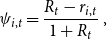
is reckoned with the following formula:
$t$
is reckoned with the following formula:
 \begin{equation} \psi _{i,t} = \frac {R_t-r_{i,t}}{1+R_t} \,, \end{equation}
and the growth rate of the Törnqvist-Theil Divisia index is defined as
 \begin{equation} log \ DM_t - log \ DM_{t-1} = \sum _{i=1}^N \bigl ({(s_{i,t}+s_{i,t-1})}/{2}\bigr) (log \ m_{i,t} - log \ m_{i,t-1}) \,, \end{equation}
where the share of asset $i$
in the Divisia index is given by
$i$
in the Divisia index is given by
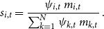 \begin{equation} s_{i,t} = \frac {\psi _{i,t} \ m_{i,t}}{\sum _{k=1}^N \psi _{k,t} \ m_{k,t}} \,. \end{equation}
Therefore, other things being equal, the more liquid a money-component asset is, the lower its return and the higher its user cost. Consequently, this asset contributes more significantly to the growth of the Divisia index.
The $DM_t$
Divisia index can be derived by compounding the growth rates from some initial normalized value. Then, correspondingly, the aggregate user cost associated with the Divisia aggregate is given by:
$DM_t$
Divisia index can be derived by compounding the growth rates from some initial normalized value. Then, correspondingly, the aggregate user cost associated with the Divisia aggregate is given by:
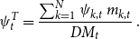 \begin{equation} \psi _t^T = \frac {\sum _{k=1}^N \psi _{k,t} \ m_{k,t}}{DM_t} \,. \end{equation}
Notice that in contrast to the Divisia index $DM_t$
, a traditional simple-sum aggregate is defined as
$DM_t$
, a traditional simple-sum aggregate is defined as $M_t = {\sum _{k=1}^N m_{k,t}}$
.
$M_t = {\sum _{k=1}^N m_{k,t}}$
.
The Center for Financial Stability (https://centerforfinancialstability.org/) calculates and publishes various Divisia indices for the United States for varying degrees of aggregation. In this paper, we use Divisia M2 (DM2) and Divisia M4 (DM4). DM2 includes currency, checking accounts, small certificates of deposit, and retail money market mutual funds. DM4 adds institutional money market funds, large negotiable certificates of deposit, overnight and term repurchase agreements, commercial paper, and US Treasury bills. These latter two assets were crucial during the Federal Reserve’s quantitative easing, highlighting the importance of using the broadest aggregate in recent empirical analyses. As supported by Kelly et al. (Reference Kelly, Barnett and Keating2011) and Keating et al. (Reference Keating, Kelly, Smith and Valcarcel2019), DM4 aggregate reflects informative content for monetary policy and monetary services from assets that were excluded from the narrower DM2. Commercial paper and US Treasury bills are still rather highly liquid and fairly safe assets used by large institutions, especially with the disintermediation of banks and the development of shadow banking.
Figure 4 shows the log-scale time paths of M2 and Divisia M2 (DM2), and those of M4 and Divisia M4 (DM4) from 1967Q1 up to 2023Q4. A visual comparison of the data reveals that despite all these series displaying long-run positive trends, their slopes, which convey their growth rates, have differed markedly in some subperiods, which suggests different characterizations of their underlying movements.
The time-paths of various monetary aggregates (in log) from 1967 to 2023.

For instance, when inflation in the early 1980s was high, the Federal Reserve under Chairman Volker is thought of as having implemented a tight monetary policy to fight inflation. Interestingly, the picture conveyed by Figure 4 differs whether the focus is on the index associated with the simple-sum aggregate or on the Divisia index. Indeed, the growth rates of M2 and M4 were strongly positive at the outset, during and after the 1981 recession, thus suggesting that, despite what was claimed and believed, the monetary policy looked expansionary. Yet, the Divisia-index counterparts for both DM2 and DM4 exhibit negative or at most flat growths preceding the recession.
In the early 1990s, both the Divisia and simple-sum indices began moving together as the Federal Reserve began targeting inflation, while interest rates were decreasing. This led to a decrease in the yield spread for all components of the money supply, causing both indices to be more in tune. What is observed, especially for M4 vs. DM4, is that as the policy interest rate was settling at lower values, the growth rate of the simple-sum aggregate slowed down, while this did not happen with DM4. This is another illustration of the difference in the information conveyed by the Divisia index versus that of the simple-sum aggregate.
During the 2008 Financial Crisis, the Federal Reserve implemented quantitative easing (QE) that increased the monetary base to increase the money supply and stimulate the economy. Surprisingly, both the Divisia and simple-sum indices did not tend to increase significantly during this period, and even decreased. This reflects the break in the money multiplier discussed earlier.
Finally, in the midst and in the aftermath of the COVID pandemic and the Great Lockdown, both the Divisia and simple-sum indices significantly increased as the Federal Reserve injected trillions of dollars into the economy with its 2020 QE program to buffer the effects of the COVID-19 pandemic. This time, the increase in the monetary base or the Fed’s balance sheet effectively affected the money supply.
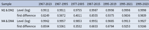
Another way to compare the relative behavior of both the levels and the growth rate of simple-sum and Divisia aggregates is to compute the contemporaneous correlations between their corresponding measures. As shown in Table 1, the M2–DM2 pair and the M4–DM4 pair in levels are highly correlated, as both simple-sum and Divisia indices share a common trend. However, the strength of the correlation, while often high and positive, is smaller with growth rates than with levels and varies across different subperiods. In particular, for the 1967–1995 subperiod, the growth rates for both the M2–DM2 pair and the M4–DM4 pair were less correlated, which corresponds to both measures seemingly signalling a different monetary policy stance. As subperiods beginning post-1987 and extending beyond 2005, the growth rates of simple-sum and Divisia indices were higher, coinciding with a period of lower interest rates and QEs. Finally, in the subperiod encompassing the onset of the pandemic and the period that followed, between 2020 and 2023, the low interest rates and the high growth of the money base led to the growth rates of both the simple-sum aggregates and the Divisia index being more highly correlated. This is consistent with Mattson and Valcarcel’s (Reference Mattson and Valcarcel2016) statistical finding that, in a period when the interest rates on all components of the aggregates are somewhat close to zero, the user cost of all components tends to fall near the same value. Since their weights in the Divisia index growth rates are very close, the evolution of the simple-sum aggregates and their Divisia index counterparts becomes somewhat more similar.
Correlations between simple-sum aggregates and their Divisia counterpart for various subsamples from 1967Q1 to 2023Q4
Barnett (Reference Barnett1980) and subsequent work in the literature have established that the Divisia indices are theoretically and conceptually superior to simple-sum aggregates. Furthermore, the difference in the information content of alternative monetary-aggregate measures and the monetary policy interest rate can have important implications for the interpretation of the monetary policy stance and its effect on the economy. To better understand the dynamics and effects of monetary policy, it seems unjustified to ignore de facto the relevance of money, as has been customary for more than three decades. Divisia measures can help deepen this relationship and provide a more accurate indication of the stance of monetary policy and the impact of the quantity of money on inflation. We now turn to a rigorous empirical evaluation of our conjecture.
4. The data and the econometric approach
4.1 The data
The dataset combines various monetary and macroeconomic variables.Footnote
12
Standard macroeconomic data, such as real GDP ( $Y_t$
), the GDP deflator (
$Y_t$
), the GDP deflator ( $P_t$
), the effective Fed Funds rate (
$P_t$
), the effective Fed Funds rate ( $FF_t$
), total reserves (
$FF_t$
), total reserves ( $TTR_t$
), non-borrowed reserves (
$TTR_t$
), non-borrowed reserves ( $NBR_t$
), the money base (
$NBR_t$
), the money base ( $MB_t$
) and the M2 aggregate (
$MB_t$
) and the M2 aggregate ( $M2_t$
), were sourced from the St. Louis Fed’s website (FRED). Divisia M2 (
$M2_t$
), were sourced from the St. Louis Fed’s website (FRED). Divisia M2 ( $DM2_t$
), Divisia M4 (
$DM2_t$
), Divisia M4 ( $DM4_t$
), and their respective user costs (
$DM4_t$
), and their respective user costs ( $UCD_t$
) were obtained from the Center for Financial Stability (CFS) website. Commodity price data (
$UCD_t$
) were obtained from the Center for Financial Stability (CFS) website. Commodity price data ( $PCOM_t$
) from 1967 to 2001 came from the CRB, and from 1972 onwards, from the Bank of Canada.Footnote
13
$PCOM_t$
) from 1967 to 2001 came from the CRB, and from 1972 onwards, from the Bank of Canada.Footnote
13
The extended sample includes periods when the effective interest rate approached the zero lower bound, prompting the Federal Reserve to use unconventional tools like quantitative easing, forward guidance, and term funding facilities. Wu and Xia’s (Reference Wu and Xia2016) shadow (Fed) Funds rate ( $SR_t$
), which can fall below 0 percent, has been proposed to better represent monetary policy during these times. Retrieved from the Atlanta Fed’s website, the shadow rate closely tracked the Fed Funds rate until 2007, but diverged significantly between 2008Q4 and 2015Q3, and between 2020Q2 and 2022Q1.
$SR_t$
), which can fall below 0 percent, has been proposed to better represent monetary policy during these times. Retrieved from the Atlanta Fed’s website, the shadow rate closely tracked the Fed Funds rate until 2007, but diverged significantly between 2008Q4 and 2015Q3, and between 2020Q2 and 2022Q1.
4.2 VAR modelling and estimation
4.2.1 The time-invariant-parameter VAR
A typical vector autoregressive representation consists of jointly modelling each variable of a system of equations as a linear function of lagged values of all the variables to capture their intrinsic built-in dynamics. It is written as
 \begin{eqnarray} \boldsymbol{\boldsymbol{{Z}}_{\boldsymbol{{t}}} = \Phi (\boldsymbol{{L}}) \, \boldsymbol{{Z}}_{\boldsymbol{{t}}-1} + \epsilon _{\boldsymbol{{t}}}}, \end{eqnarray}
where $\boldsymbol{{Z}}_{\boldsymbol{{t}}} = [z_{1,t}, \ldots, z_{Q,t}]^{\prime}$
is the vector of variables and
$\boldsymbol{{Z}}_{\boldsymbol{{t}}} = [z_{1,t}, \ldots, z_{Q,t}]^{\prime}$
is the vector of variables and $\boldsymbol{\epsilon}_{\boldsymbol{{t}}} = [\epsilon_{1,t}, \ldots, \epsilon_{Q,t}]^{\prime}$
is a vector white noise process, i.e.,
$\boldsymbol{\epsilon}_{\boldsymbol{{t}}} = [\epsilon_{1,t}, \ldots, \epsilon_{Q,t}]^{\prime}$
is a vector white noise process, i.e., $E(\boldsymbol{\epsilon} _{\boldsymbol{{t}}}) = \boldsymbol{0}, \, E(\boldsymbol{\epsilon _{\boldsymbol{{t}}} \, \epsilon _t^{\prime}}) = \boldsymbol{\Omega_\epsilon}, \text{ and } E(\boldsymbol{\epsilon} _{\boldsymbol{{t}}}\, \boldsymbol{\epsilon} _{\boldsymbol{{s}}}^{\prime}) = \boldsymbol{0}$
for any
$E(\boldsymbol{\epsilon} _{\boldsymbol{{t}}}) = \boldsymbol{0}, \, E(\boldsymbol{\epsilon _{\boldsymbol{{t}}} \, \epsilon _t^{\prime}}) = \boldsymbol{\Omega_\epsilon}, \text{ and } E(\boldsymbol{\epsilon} _{\boldsymbol{{t}}}\, \boldsymbol{\epsilon} _{\boldsymbol{{s}}}^{\prime}) = \boldsymbol{0}$
for any $t \neq s$
. The parameters making up the matrices in the K-order lag-matrix polynomials in
$t \neq s$
. The parameters making up the matrices in the K-order lag-matrix polynomials in $\boldsymbol{\Phi} (\boldsymbol{{L}})$
are assumed to be time invariant.
$\boldsymbol{\Phi} (\boldsymbol{{L}})$
are assumed to be time invariant.
Once the order of the VAR system is established on empirical ground, with the absence of serial correlation in its residuals, the VAR’s time-invariant parameters can be estimated consistently and efficiently by maximum likelihood, which is equivalent to the application of OLS applied separately to each equation, in the situation when all the system’s equations share the same regressors, which amounts to solve
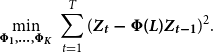 \begin{eqnarray} \underset {\boldsymbol{\Phi_{1},\ldots,\Phi _{\boldsymbol{{K}}}}}{\textrm {min}}\, \sum_{t=1}^T (\boldsymbol{\boldsymbol{{Z}}_{\boldsymbol{{t}}} - \Phi (\boldsymbol{{L}}) \boldsymbol{{Z}}_{\boldsymbol{{t}}-1}})^{2}. \end{eqnarray}
As commonly used in the literature and explained in section 4.3, the VAR model also amounts to the reduced form of an underlying structural model that can be recovered once one imposes a required number of reasonable identifying restrictions.
4.2.2 The time-varying-parameter VAR
Changes in the economic environment and various financial innovations over the years that have led to the creation and use of new assets, as well as changes in monetary transmission, may well have impacted the dynamics between macroeconomic variables. To account for the possibility that the underlying dynamic relationships may have changed across variables in a model and may have evolved over time, a logical extension to model structural changes in economics is to consider a time-varying-parameter vector autoregressive (TVP-VAR) representation explicitly, such as:
 \begin{eqnarray}\boldsymbol{\boldsymbol{{Z}}_{\boldsymbol{{t}}} = \Phi_{\boldsymbol{{t}}}(\boldsymbol{{L}})\boldsymbol{{Z}}_{\boldsymbol{{t}}-1} + \epsilon_{\boldsymbol{{t}}}, \ \epsilon _{\boldsymbol{{t}}}\thicksim\mathrm{N}(0,\Omega _{\epsilon _{\boldsymbol{{t}}}}) }, \end{eqnarray}
 \begin{eqnarray} \boldsymbol{\Phi_{\boldsymbol{{t}}} = \Phi _{\boldsymbol{{t}}-1} +\boldsymbol{{e}}_{\boldsymbol{{t}}}, \boldsymbol{{e}}_{\boldsymbol{{t}}}\thicksim\mathrm{N}(0,\Omega _{\boldsymbol{{e}}})}, \end{eqnarray}
where $\boldsymbol{\Phi_{\boldsymbol{{t}}}(\boldsymbol{{L}})}$
is a
$\boldsymbol{\Phi_{\boldsymbol{{t}}}(\boldsymbol{{L}})}$
is a $K^{th}$
-order matrixlag polynomial, whose sequence of matrix coefficients are given by
$K^{th}$
-order matrixlag polynomial, whose sequence of matrix coefficients are given by $\boldsymbol{\Phi _{1,\boldsymbol{{t}}},\ldots,\Phi _{\boldsymbol{{K}},\boldsymbol{{t}}}}$
.
$\boldsymbol{\Phi _{1,\boldsymbol{{t}}},\ldots,\Phi _{\boldsymbol{{K}},\boldsymbol{{t}}}}$
.
As shown by Primiceri (Reference Primiceri2005), a model akin to that above, assuming amultivariate stochastic volatility, can be estimated using Bayesianestimation. Essentially, the procedure starts with conditional priordistributions for the unknown parameters associated with the vectorsin $\boldsymbol{\Phi_{\boldsymbol{{t}}}(\boldsymbol{{L}})}$
and their covariance matrices
$\boldsymbol{\Phi_{\boldsymbol{{t}}}(\boldsymbol{{L}})}$
and their covariance matrices $\boldsymbol{\Omega _{\epsilon _{\boldsymbol{{t}}}}}$
. By combining the likelihood function with some informative prior distributions based on initial beliefs, Bayes’ theorem updates these priors with new data to form the posterior density distribution, reflecting updated beliefs. The parameters of the prior distributions, called hyperparameters, control the shape and scale of the priors and can influence the model’s flexibility and robustness. The TVP-BVAR employs Markov Chain Monte Carlo (MCMC) techniques on an expanding window of data. The Gibbs sampler is utilized to generate multivariate posterior distributions of the model parameters.
$\boldsymbol{\Omega _{\epsilon _{\boldsymbol{{t}}}}}$
. By combining the likelihood function with some informative prior distributions based on initial beliefs, Bayes’ theorem updates these priors with new data to form the posterior density distribution, reflecting updated beliefs. The parameters of the prior distributions, called hyperparameters, control the shape and scale of the priors and can influence the model’s flexibility and robustness. The TVP-BVAR employs Markov Chain Monte Carlo (MCMC) techniques on an expanding window of data. The Gibbs sampler is utilized to generate multivariate posterior distributions of the model parameters.
As argued by Goulet Coulombe (Reference Goulet Coulombe2025), one difficulty that arises in the estimation of a TVP-VAR relates to “tuning the crucial amount of time variation” in the elements of the $\boldsymbol{\Phi _{i,\boldsymbol{{t}}}}$
matrices, for
$\boldsymbol{\Phi _{i,\boldsymbol{{t}}}}$
matrices, for $i=1, \ldots, K$
. Alternatively, he showed that multivariate random walk TVPs such as the system defined by equation (8) and (9) give rise to a multivariate TVP-ridge problem, which is particularly useful to obtain point estimates, on which we will focus. Accordingly, he showed how to carry the estimation of the empirical model by multivariate Two-Step Ridge Regression (2SRR) that amounts to solving
$i=1, \ldots, K$
. Alternatively, he showed that multivariate random walk TVPs such as the system defined by equation (8) and (9) give rise to a multivariate TVP-ridge problem, which is particularly useful to obtain point estimates, on which we will focus. Accordingly, he showed how to carry the estimation of the empirical model by multivariate Two-Step Ridge Regression (2SRR) that amounts to solving
 \begin{eqnarray} \underset {\boldsymbol{\Phi _{1,\boldsymbol{{t}}},\ldots,\Phi _{\boldsymbol{{K}},\boldsymbol{{t}}}}}{\min } \, \sum _{t=1}^T (\boldsymbol{\boldsymbol{{Z}}_{\boldsymbol{{t}}} - \Phi _{\boldsymbol{{t}}}(\boldsymbol{{L}}) \boldsymbol{{Z}}_{\boldsymbol{{t}}-1}})^2 + \sum _{k=1}^K \sum _{t=1}^T \lambda _k \parallel \boldsymbol{\Phi _{\boldsymbol{{k}},\boldsymbol{{t}}} - \Phi _{\boldsymbol{{k}},\boldsymbol{{t}}-1}}\parallel ^2 \end{eqnarray}
and $ \boldsymbol{{Z}}_{\boldsymbol{{t}}}$
is the
$ \boldsymbol{{Z}}_{\boldsymbol{{t}}}$
is the $Q \times 1$
vector of variables.
$Q \times 1$
vector of variables.
The required computations are carried out via a closed-form solution in the form of data-augmented ridge regression. Throughout the estimation process, the 2SRR method carefully considers key aspects to ensure robustness and mitigate overfitting.
In the 2SRR framework, the smoothing $\lambda _k$
-hyperparameters drive the amount of time variation in the VARs coefficients and aim at optimally balancing bias and variance, as they are functions of the ratio of the variances of
$\lambda _k$
-hyperparameters drive the amount of time variation in the VARs coefficients and aim at optimally balancing bias and variance, as they are functions of the ratio of the variances of $\boldsymbol{\epsilon _{\boldsymbol{{t}}}}$
and
$\boldsymbol{\epsilon _{\boldsymbol{{t}}}}$
and $\boldsymbol{\boldsymbol{{e}}_{\boldsymbol{{t}}}}$
. Goulet Coulombe (Reference Goulet Coulombe2025) proposed a data-driven choice for the
$\boldsymbol{\boldsymbol{{e}}_{\boldsymbol{{t}}}}$
. Goulet Coulombe (Reference Goulet Coulombe2025) proposed a data-driven choice for the $\lambda _k$
’s values based on blocked 5-fold cross-validations for quarterly data, which accounts for time dependence between data points and avoids overfitting issues. The selected block size of 10 quarters strikes a balance between capturing relevant time information and preventing excessive dimensionality.
$\lambda _k$
’s values based on blocked 5-fold cross-validations for quarterly data, which accounts for time dependence between data points and avoids overfitting issues. The selected block size of 10 quarters strikes a balance between capturing relevant time information and preventing excessive dimensionality.
Moreover, his comparisons for different scenarios characterized by distinct patterns of time-varying parameters and varying proportions within the total parameter space confirmed that the performance of 2SRR in accurately capturing the dynamic path of true parameters closely aligned with that of the standard Bayesian TVP-VAR with stochastic volatility.
In a manner akin to that used with time-invariant VARs, identifying restrictions will make it possible to retrieve structural shocks and their implied dynamic impacts on the empirical model’s variables, albeit accounting for time variation in both the sizes of shocks and the variables’ responses.
4.2.3 Contrasting Bayesian and 2SRR estimators for TVP-VAR models
Until now, the empirical literature has employed Bayesian inference to estimate TVP-VAR models (TVP-BVAR), while this paper makes use of the 2SRR estimator recently proposed by Goulet Coulombe (Reference Goulet Coulombe2025), who found that both methods yield comparable effectiveness in estimating the dynamics of the variables, albeit each has distinct features in their application with a given sample.
TVP-BVAR estimation allows the integration of prior beliefs or information, which can be valuable when data is sparse and noisy, but it tends to be computationally intensive. However, their results may be sensitive to the choice of priors and may lead to misleading inferences. TVP-BVAR estimation using MCMC requires setting values of key hyperparameters, which often leads practitioners to use values somewhat consistent with those in Primiceri (Reference Primiceri2005) or Giannone et al. (Reference Giannone, Lenza and Primiceri2015).Footnote 14 Moreover, TVP-BVAR requires a lengthy enough “initial training sample period” to initialize the specifications in order to reliably estimate the time-varying parameters and their evolution. Hence, estimates obtained from TVP-BVAR are contingent on data that predates the results for a reported sample.Footnote 15 Finally, conducting the Bayesian estimation with MCMC requires building a Markov chain that has a joint stationary distribution from which the parameter estimates can be sampled. To ensure the convergence of the distribution, this can be done by discarding a sufficient number of initial samples to let the simulated distribution stabilize.Footnote 16
By contrast, the 2SRR estimation of TVP-VAR does not involve burdensome MCMC simulations. It only needs to determine the time-smoothing $\lambda _k$
-hyperparameters, which define the extent of time variation without the initialization and convergence issues pertaining to Bayesian TVP-VARs. These practical considerations, linked to the treatment of numerous hyperparameters and the loss of observations inherent to the Bayesian estimation, confer advantages that motivate the use of the newest 2SRR estimator to account for time-varying parameters in the VAR models.
$\lambda _k$
-hyperparameters, which define the extent of time variation without the initialization and convergence issues pertaining to Bayesian TVP-VARs. These practical considerations, linked to the treatment of numerous hyperparameters and the loss of observations inherent to the Bayesian estimation, confer advantages that motivate the use of the newest 2SRR estimator to account for time-varying parameters in the VAR models.
4.3 Structural VAR and identification
The basic time-invariant VAR in equation (6) for the vector of endogenous variables $\boldsymbol{\boldsymbol{{Z}}}_t$
can be thought of as the reduced form of an underlying structural model such as:
$\boldsymbol{\boldsymbol{{Z}}}_t$
can be thought of as the reduced form of an underlying structural model such as:
 \begin{eqnarray} \boldsymbol{\boldsymbol{{A}}_0 \, \boldsymbol{{Z}}_{\boldsymbol{{t}}} = \boldsymbol{{B}}(\boldsymbol{{L}}) \, \boldsymbol{{Z}}_{\boldsymbol{{t}}-1} + \boldsymbol{{u}}_{\boldsymbol{{t}}}} \end{eqnarray}
where the $\boldsymbol{\boldsymbol{{A}}_0}$
matrix captures the contemporaneous endogeneity between the variables in
$\boldsymbol{\boldsymbol{{A}}_0}$
matrix captures the contemporaneous endogeneity between the variables in $\boldsymbol{\boldsymbol{{Z}}}_t$
, while the
$\boldsymbol{\boldsymbol{{Z}}}_t$
, while the $p$
-order lag-matrix polynomial in
$p$
-order lag-matrix polynomial in $\boldsymbol{\boldsymbol{{B}}(\boldsymbol{{L}})}$
represents the intrinsic dynamics built-in for the endogenous variables of the system, and
$\boldsymbol{\boldsymbol{{B}}(\boldsymbol{{L}})}$
represents the intrinsic dynamics built-in for the endogenous variables of the system, and $\boldsymbol{\boldsymbol{{u}}}_t$
is the vector of (orthogonal) structural shocks driving the endogenous variables.
$\boldsymbol{\boldsymbol{{u}}}_t$
is the vector of (orthogonal) structural shocks driving the endogenous variables.
Accordingly, the VAR or reduced form of the system in equation (11) is given by:
 \begin{eqnarray} \boldsymbol{\boldsymbol{{Z}}_{\boldsymbol{{t}}} = \boldsymbol{{A}}_0^{-1} \, \boldsymbol{{B}}(\boldsymbol{{L}}) \, \boldsymbol{{Z}}_{\boldsymbol{{t}}-1} + \boldsymbol{{A}}_0^{-1} \, \boldsymbol{{u}}_{\boldsymbol{{t}}} = \Phi (\boldsymbol{{L}}) \, \boldsymbol{{Z}}_{\boldsymbol{{t}}-1} + \varepsilon _{\boldsymbol{{t}}}} \end{eqnarray}
with the vector of reduced-form residuals $\boldsymbol{\varepsilon _{\boldsymbol{{t}}} = \boldsymbol{{A}}_0^{-1} \, \boldsymbol{{u}}_{\boldsymbol{{t}}}}$
, and which admits the following equivalent VMA(
$\boldsymbol{\varepsilon _{\boldsymbol{{t}}} = \boldsymbol{{A}}_0^{-1} \, \boldsymbol{{u}}_{\boldsymbol{{t}}}}$
, and which admits the following equivalent VMA( $\infty$
) representation:
$\infty$
) representation:
 \begin{eqnarray} \boldsymbol{{Z}}_{\boldsymbol{{t}}} &=& \boldsymbol{[\boldsymbol{{I}} - \Phi (\boldsymbol{{L}}) \, \boldsymbol{{L}}]^{-1} \, \boldsymbol{{A}}_0^{-1} \, \boldsymbol{{u}}_{\boldsymbol{{t}}}} = \boldsymbol{\Psi (\boldsymbol{{L}}) \, \, \boldsymbol{{u}}_{\boldsymbol{{t}}}}. \end{eqnarray}
Since $\boldsymbol{\boldsymbol{{u}}_{\boldsymbol{{t}}} = \boldsymbol{{A}}_0 \, \varepsilon _{\boldsymbol{{t}}}}$
, therefore:
$\boldsymbol{\boldsymbol{{u}}_{\boldsymbol{{t}}} = \boldsymbol{{A}}_0 \, \varepsilon _{\boldsymbol{{t}}}}$
, therefore:
 \begin{eqnarray} \boldsymbol{\Sigma _{\boldsymbol{{u}}} = \boldsymbol{{E}}[\boldsymbol{{u}}_{\boldsymbol{{t}}} \boldsymbol{{u}}_{\boldsymbol{{t}}}^{\prime}] = \boldsymbol{{A}}_0 \, \boldsymbol{{E}}[\varepsilon _{\boldsymbol{{t}}} \varepsilon _{\boldsymbol{{t}}}^{\prime}] \, \boldsymbol{{A}}_0^{\prime} = \boldsymbol{{A}}_0 \, \Sigma _\varepsilon \, \boldsymbol{{A}}_0^{\prime} }. \end{eqnarray}
By imposing enough identification restrictions on the matrix equation above, it is possible to recover the $\boldsymbol{\boldsymbol{{A}}_0}$
matrix. Then, the proper elements of the
$\boldsymbol{\boldsymbol{{A}}_0}$
matrix. Then, the proper elements of the $\boldsymbol{\Psi (\boldsymbol{{L}})}$
matrix polynomial can be used to plot the dynamic or impulse responses of the structural shocks in
$\boldsymbol{\Psi (\boldsymbol{{L}})}$
matrix polynomial can be used to plot the dynamic or impulse responses of the structural shocks in $\boldsymbol{\boldsymbol{{u}}_{\boldsymbol{{t}}}}$
, and to calculate their contribution to the variance of different variables at different horizons.
$\boldsymbol{\boldsymbol{{u}}_{\boldsymbol{{t}}}}$
, and to calculate their contribution to the variance of different variables at different horizons.
Given a particular and reasonable set of identification restrictions, the structural VAR approach provides an interpretation of the impulse response functions (IRFs) for the model with, for instance, the dynamic response of the variables to a one-time structural shock to the monetary-policy signalling variable.Footnote 17 Finally, even within the class of short-run identifying restrictions, it is necessary to make the case for the transmission channel of the shocks of interest.
In a manner akin to that used for the time-invariant VAR, imposing identifying restrictions on the estimated TVP-VARs by 2SRR yields estimates of time-varying impulse response functions.Footnote 18
Once we have settled on a relevant and reasonable set of identification restrictions, the IRFs can be used to evaluate the effectiveness of different monetary policy strategies and to inform policymakers about the potential impact of their decisions on the economy. Because of the alternative and possibly unresolved debate about which variable is empirically the most appropriate indicator to extract the stance of monetary policy, we will compare results for multiple monetary policy indicator variables, and assess their ability and reasonableness in capturing the dynamics of macroeconomic variables.
One popular method for identifying the structural shocks in a SVAR model consists of imposing restrictions on the short-term coefficient matrix with a block recursive identification approach, such as in the seminal paper by Christiano et al. (Reference Christiano, Eichenbaum, Evans, Christiano, Eichenbaum and Evans1999). In this paper, the authors use a three-block variable SVAR model to study the effects of a monetary policy shock on output, inflation, and other economic variables. The block recursive identification approach, which is akin to the Cholesky decomposition, involves partitioning the variables in the model into blocks, based on economic theory or prior knowledge of the relationships between the variables. The variables within each block are ordered based on their causal relationships, and the shocks are identified recursively by imposing restrictions on the lower-triangular covariance matrix of the error terms in the model.
The block-recursive restrictions amount to the following structural specification of the matrix associated with the contemporaneous relationships between the model’s variables:
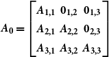 \begin{eqnarray} \boldsymbol{\boldsymbol{{A}}_0 = \begin{bmatrix} \boldsymbol{\boldsymbol{{A}}_{1,1}} & \boldsymbol{0_{1,2}} & \boldsymbol{0_{1,3}} \\ \boldsymbol{\boldsymbol{{A}}_{2,1}} & \boldsymbol{\boldsymbol{{A}}_{2,2}} & \boldsymbol{0_{2,3}} \\ \boldsymbol{\boldsymbol{{A}}_{3,1}} & \boldsymbol{\boldsymbol{{A}}_{3,2}} & \boldsymbol{\boldsymbol{{A}}_{3,3}} \\ \end{bmatrix}} \end{eqnarray}
with the matrix of variables being partitioned as $\boldsymbol{\boldsymbol{{Z}}_{\boldsymbol{{t}}} = [ \ \boldsymbol{{X}}_{1,\boldsymbol{{t}}}^{\prime} \ \ \boldsymbol{{S}}_{\boldsymbol{{t}}}^{\prime} \ \ \boldsymbol{{X}}_{2,\boldsymbol{{t}}}^{\prime}\ {]}^{\prime}}$
.
$\boldsymbol{\boldsymbol{{Z}}_{\boldsymbol{{t}}} = [ \ \boldsymbol{{X}}_{1,\boldsymbol{{t}}}^{\prime} \ \ \boldsymbol{{S}}_{\boldsymbol{{t}}}^{\prime} \ \ \boldsymbol{{X}}_{2,\boldsymbol{{t}}}^{\prime}\ {]}^{\prime}}$
.
The first block includes macroeconomic variables that respond to a monetary policy shock with a one-lag delay, such as real GDP, the implicit GDP deflator index, and the commodity price index. The second block comprises the monetary policy variable indicator, such as an interest rate or a monetary aggregate. The third block contains money market variables that immediately react to the monetary policy shock, such as reserves, the monetary base, or a monetary aggregate.
In the empirical literature, the Fed Funds rate has, by and large, mostly been favored as the signalling variable to extract a monetary shock indicating the direction of monetary policy. This is also consistent with that variable being generally preferred by the Federal Reserve to communicate its intent and decision regarding monetary policy.
Using monthly and quarterly data from 1965M1 to 1995M6, Christiano et al.’s (Reference Christiano, Eichenbaum, Evans, Christiano, Eichenbaum and Evans1999) preferred VAR specification defined the matrix of variables and its identifying restriction ordering according to $\boldsymbol{{Z}}_{\boldsymbol{{t}}} = [Y_t, P_t, PCOM_t, S_t, NBR_t, TTR_t, M2_t]$
. They found the federal funds rate to be the superior indicator variable, showing a strong negative response of GDP and an eventual reduction in the price level following a restrictive monetary policy shock, with fewer empirical puzzles compared to some reserve money or a money aggregate.
$\boldsymbol{{Z}}_{\boldsymbol{{t}}} = [Y_t, P_t, PCOM_t, S_t, NBR_t, TTR_t, M2_t]$
. They found the federal funds rate to be the superior indicator variable, showing a strong negative response of GDP and an eventual reduction in the price level following a restrictive monetary policy shock, with fewer empirical puzzles compared to some reserve money or a money aggregate.
In Keating et al. (Reference Keating, Kelly, Smith and Valcarcel2019), the non-borrowed reserves and total reserves were replaced by the monetary base because NBR went negative during the Great Recession. Moreover, their ordering used for identification is $ \boldsymbol{{Z}}_{\boldsymbol{{t}}} = [Y_t, P_t, PCOM_t, S_t, MB_t, \varnothing \ {or} \ M2_t \ {or} \ UCD_t]$
. In a sample from 1967Q1 to 2015Q4, they found that a Divisia index is a superior monetary policy indicator compared to the Fed Funds rate or a shadow rate, especially before and after the use of quantitative easing during the 2008 Great Recession. Following a monetary policy shock, their dynamic responses do not show empirical puzzles regarding price, output, or the interest rate. Chen and Valcarcel (Reference Chen and Valcarcel2021) reported similar findings over the 1988M10-2020M2 sample.
$ \boldsymbol{{Z}}_{\boldsymbol{{t}}} = [Y_t, P_t, PCOM_t, S_t, MB_t, \varnothing \ {or} \ M2_t \ {or} \ UCD_t]$
. In a sample from 1967Q1 to 2015Q4, they found that a Divisia index is a superior monetary policy indicator compared to the Fed Funds rate or a shadow rate, especially before and after the use of quantitative easing during the 2008 Great Recession. Following a monetary policy shock, their dynamic responses do not show empirical puzzles regarding price, output, or the interest rate. Chen and Valcarcel (Reference Chen and Valcarcel2021) reported similar findings over the 1988M10-2020M2 sample.
Except for one comparison with Christiano et al. (Reference Christiano, Eichenbaum, Evans, Christiano, Eichenbaum and Evans1999) over the 1967Q1–1995Q2 period, we use the same ordering as in Keating et al. (Reference Keating, Kelly, Smith and Valcarcel2019) for identifying structural monetary policy shocks, with quarterly data for a full sample, as well as subsamples, up to 2023Q4. This sample includes data from the recent “natural experiment” episode, marked by expansionary monetary policy during the pandemic, followed by inflation and a policy shift to bring inflation back to 2%. Table 2 lists the variables in their original form in our SVAR model.
Variables used in the empirical VAR models
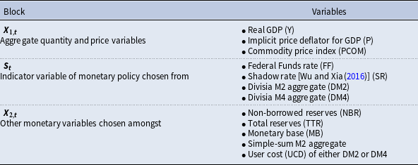
Note: Except for interest rates, all variables are expressed in log.
4.4 Assessment of out-of-sample point forecasts and implications for competing models
Since we will be comparing the IRFs of structural models that include either the Fed Funds rate, a shadow rate, a conventional monetary aggregate or its Divisia counterpart, it is worth discussing the extent to which the forecasting capacity of various models may be relevant to judge the reasonability and relevance of the IRFs under consideration. Indeed, the information content of a monetary policy indicator hinges on its consistent usefulness and contribution in out-of-sample (OOS) forecasting.
In econometric modelling, impulse response functions trace the dynamic effects on key variables following a structural shock to a given variable, similar to a conditional forecast. As such, they serve as valuable tools for understanding the system’s response to shocks. Their construction relies upon the assumption that the model is able to capture the dynamics of the underlying data generating process (DGP).
The robustness of estimated IRFs depends on the model’s economic foundations, grounded in a thoughtful selection of variables, its specification and identifying restrictions aligned with the true underlying DGP. At the same time, factual accuracy of IRFs must translate into good forecasting performance. Hence, a model’s empirical reliability should rest on predictive accuracy that complements a sound understanding of the economic mechanisms it seeks to capture. This can enhance the overall relevance of the model’s implications, as the IRFs could provide a useful depiction of the underlying economic reality, even though a good forecasting model without a good understanding of the underlying economic mechanisms would not guarantee the dependability of the IRFs.
Thus, when comparing two models with variables deemed to represent the same policy context and characteristics, using similar identifying restrictions/ordering, a reduction in the dispersion of the OOS forecast errors may be interpreted as reflecting a closer alignment of the empirical model to the actual underlying DGP. This is the motivation for gauging and contrasting the predictive accuracy of our different specifications with alternative monetary policy indicators.
Thereby, we proceed to pseudo-OOS point forecasts analyses from 1- to 8-quarters ahead, spanning the period from the first quarter of 2011 to the fourth quarter of 2023, and from the first quarter of 2020 to the fourth quarter of 2023 for the variables.Footnote
19
The recursive estimation and tuning of the models at each stage is used to construct the predicted value of the variables, using an expanding window estimated from the first quarter of 1967. The Root Mean Square Prediction Error (RMSPE), which is a standard metric in the literature, was used to assess the degree of forecast accuracy. Accordingly, for the OOS forecasted values at time $t$
of variable
$t$
of variable $v$
made
$v$
made $h$
-steps ahead from model
$h$
-steps ahead from model $j$
, i.e.,
$j$
, i.e., $\hat {y}{}_{t}^{v,h,j}$
, the relevant quantities are computed as
$\hat {y}{}_{t}^{v,h,j}$
, the relevant quantities are computed as
 \begin{eqnarray} RMSPE_{v,h,j} = \sqrt {\frac {1}{\#OOS} \sum _{t \, \epsilon \, OOS} {(y_{t+h}^v - \hat {y}{}_{t}^{v,h,j})}^2} \,. \end{eqnarray}
Each variable, step-ahead forecast, and model specification combination yields a unique RMSPE value. Then, the values of the RMSPE for a given $\hat {y}_{t}^{v,h,j}$
are expressed in relative terms by calculating the ratio of the RMSPE for a particular forecasting model
$\hat {y}_{t}^{v,h,j}$
are expressed in relative terms by calculating the ratio of the RMSPE for a particular forecasting model $j$
to that of some reference model. For all variables, we will use the RMSPE of forecasts from an AR(2) as the reference model, as this simple univariate model is often considered as producing good forecasts for various macroeconomic variables (e.g., see Goulet Coulombe (Reference Goulet Coulombe2025), amongst others). The normalization of the RMSPE scores for each model against those of a benchmark model, for each variable and every forecasting horizon, facilitates relative comparisons across specifications with alternate monetary policy indicators. A value below 1 indicates that a model surpasses the benchmark for that specific variable and
$j$
to that of some reference model. For all variables, we will use the RMSPE of forecasts from an AR(2) as the reference model, as this simple univariate model is often considered as producing good forecasts for various macroeconomic variables (e.g., see Goulet Coulombe (Reference Goulet Coulombe2025), amongst others). The normalization of the RMSPE scores for each model against those of a benchmark model, for each variable and every forecasting horizon, facilitates relative comparisons across specifications with alternate monetary policy indicators. A value below 1 indicates that a model surpasses the benchmark for that specific variable and $h$
-steps-ahead forecasting horizon. However, regardless of a specific value, the forecasting accuracy of different models can still be compared with one another.Footnote
20
$h$
-steps-ahead forecasting horizon. However, regardless of a specific value, the forecasting accuracy of different models can still be compared with one another.Footnote
20
Finally, the pseudo-OOS analysis is conducted using violin plots to represent the density of the normalized distribution of the RMSPEs. These are drawn after applying a kernel density estimator to the normalized values of the RMSPEs. These plots facilitate the visualization of the degree of each model’s forecasting accuracy by showing whether the RMSPEs are clustered in the same region or whether they exhibit a wide dispersion.
5. The empirical results
5.1 The out-of-sample forecast assessment of time-invariant VAR specifications
Based on the Akaike Information Criterion (AIC) and the Bayesian Information Criterion (BIC) for the whole sample and the various subsamples considered, as well as on unit root tests, stationary considerations, and tests for no autocorrelation, we selected a 5-quarter lag length for our VARs. That is the same number of lags as in Keating et al. (Reference Keating, Kelly, Smith and Valcarcel2019), and one more lag than in Christiano et al. (Reference Christiano, Eichenbaum, Evans, Christiano, Eichenbaum and Evans1999).Footnote 21 Except for the interest rates, the variables are in logs and first-differenced for stationarity when data past 2008 were in the sample. This is in accordance with the requirement that the eigenvalues of the companion matrix associated with the VAR coefficients lie within the unit circle, and with augmented Dickey-Fuller tests.Footnote 22
We now turn to a comparison of the OOS point forecast performance of the alternative monetary policy indicator in VAR modelling. A better forecasting model is at least indicative of the relevance of the information content revealed by its variables. Hence, to the extent that models including measures of the “quantity of money” exhibit more accurate forecasting, this lends support for their consideration in measuring monetary policy shocks and in assessing their impact on key macroeconomic variables.
As explained earlier, after an initial estimation for the 1967Q1-2010Q4 sample, subsequent estimations were performed with a sequence of extended samples that cover up to 2023Q4, so that the RMSPEs for the pseudo-OOS forecasts of the variables of interest from 1- to 8-quarters ahead for all subsamples from 2011Q1 up to 2023Q4 were constructed for each model and divided by the corresponding RMSPEs reckoned with a univariate AR(2) model. Violin plots were then generated to illustrate the distribution of the degree of forecasting accuracy for each specification over both 2011Q1–2023Q4 and 2020Q1–2023Q4. The latter period isolates the period that includes the COVID pandemic.
The width of a violin along the vertical axis conveys the density of the RMSPE values, providing an immediate grasp of the variability and central tendencies inherent in the predictive performance of each model. A wider violin along the horizontal axis suggests a consistent forecasting performance, while a model whose violins have narrower and taller peaks implies that its forecasting performance is less stable. The horizontal line within each violin represents the median normalized RMSPE value. Thus, other things being equal, a shorter and wider violin that lies generally lower in the plot outperforms its rivals.
Seven specifications were considered for the empirical models. In each one, the first block includes real GDP (Y), the implicit GDP deflator (P), and commodity prices. In the second block, the monetary policy indicator variable $S_t$
is defined as either DM4, the Fed Funds rate (FF), or the shadow rate (SR). For models with policy rates, the third block counts the monetary base (MB) either alone, with M2, or with DM2. For models with DM4, the monetary base and the user cost of DM4 are in the third block. The results of the comparisons for forecasts made with time-invariant parameter VARs are presented in Figure 5.
$S_t$
is defined as either DM4, the Fed Funds rate (FF), or the shadow rate (SR). For models with policy rates, the third block counts the monetary base (MB) either alone, with M2, or with DM2. For models with DM4, the monetary base and the user cost of DM4 are in the third block. The results of the comparisons for forecasts made with time-invariant parameter VARs are presented in Figure 5.
Relative RMSPE performance of pseudo-out-of-sample 1- to 8-quarters-ahead forecasts over 2011Q1–2023Q4 and 2020Q1–2023Q4 from time-invariant parameter VARs.
The vertical axis reports the ratio of the RMSPE from a particular forecasting model to the RMSPE from an AR(2), as the reference model, to compare the relative performance of alternative specifications. Seven specifications were considered. The label at the bottom of each violin shows the monetary indicator $S_t$
that was included. Moreover, in curly brackets, when applicable, it indicates whether M2
$S_t$
that was included. Moreover, in curly brackets, when applicable, it indicates whether M2 $_t$
or DM2
$_t$
or DM2 $_t$
was included within the third block of variables in addition to MB
$_t$
was included within the third block of variables in addition to MB $_t$
when the monetary indicator was either the Fed Funds rate or the shadow rate.
$_t$
when the monetary indicator was either the Fed Funds rate or the shadow rate.
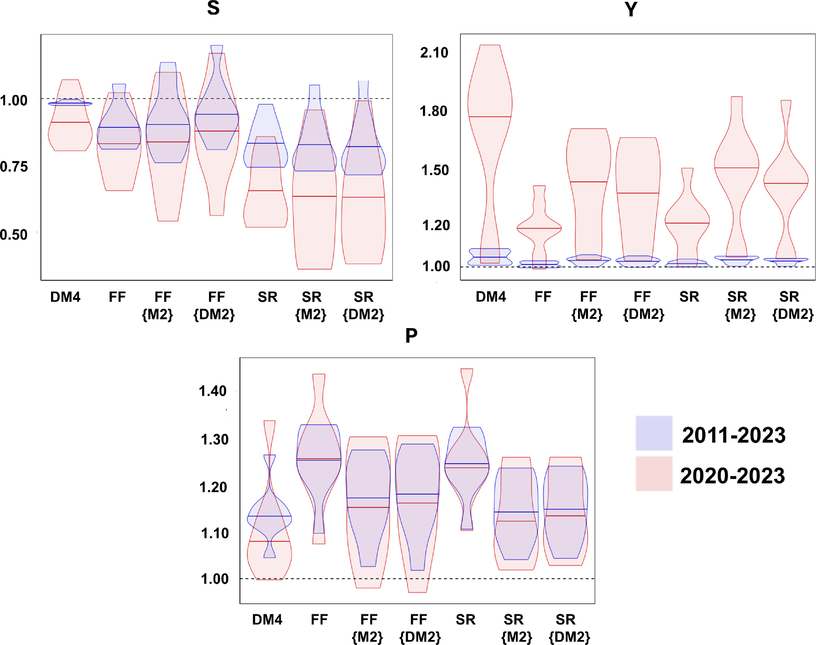
As the first panel of the figure refers to forecasts of different policy indicator variables $S_t$
, it does not make a direct performance comparison on the same footing. Nonetheless, the median RMSPEs suggest that it is easier to forecast the Fed Funds rate or the shadow rate than DM4, albeit the RMSPEs are generally more dispersed for the policy rate variables than for DM4. Moreover, there are some indications that adding either M2 or DM2 to the VARs associated with the policy rates may improve their forecasts, which are denoted by the apposed label between curly brackets.
$S_t$
, it does not make a direct performance comparison on the same footing. Nonetheless, the median RMSPEs suggest that it is easier to forecast the Fed Funds rate or the shadow rate than DM4, albeit the RMSPEs are generally more dispersed for the policy rate variables than for DM4. Moreover, there are some indications that adding either M2 or DM2 to the VARs associated with the policy rates may improve their forecasts, which are denoted by the apposed label between curly brackets.
For output and prices, the median relative RMSPE for the variables of interest is greater than one for all specifications, indicating that the quality of the forecasts from a simple univariate AR(2) surpasses that of a VAR with fixed coefficients. However, our purpose is not to uncover the best overall forecasting model. Rather, it is to compare the information content and dynamics revealed by models that include or abstract from money.
For real GDP, the violin plots suggest that the information content for future output is better divulged from models with policy rates than from a model with DM4. The difference is relatively small when considering the whole 2011–2023 period, but it is more significative for the 2020–2023 period, with the focus on the COVID recession. For the price level, the forecasting accuracy of models that include the Fed Funds rate or the shadow rate without a money aggregate does not fare well in either forecasting period. However, the forecasting performance for P with the policy rate variables is much improved when the corresponding VAR includes either M2, or DM2. Overall, the DM4 specification globally exhibits the most accurate forecasts for the price level.
Better forecast accuracy, as shown by lower RMSPEs, does not automatically mean that the IRFs are more robust for analyzing monetary policy dynamics. However, if the identification restrictions match a structural model that accurately reflects the data generation process, then a model with superior forecasting ability is likely to provide more reliable and sensible response functions.Footnote 23 In that sense, the IRFs estimated from VAR models with DM4 may logically tend to be more robust.
5.2 Evidence from time-invariant impulse response functions for different specifications and periods
This section presents an analysis of the response of economic variables to a restrictive monetary policy shock. Our aim is to examine the response functions using alternative monetary policy shocks extracted from different indicator variables. We thus seek to better understand the transmission mechanisms of monetary policy and to assess potential variations in their impact on the economy.
As mentioned earlier, the estimation relied on fifth-order time-invariant VAR models.Footnote 24 The confidence intervals for the impulse response functions were estimated using the bootstrap Monte Carlo method, as in Christiano et al. (Reference Christiano, Eichenbaum, Evans, Christiano, Eichenbaum and Evans1999). As the null hypothesis of the absence of autocorrelation in the residuals was not rejected, the estimated residuals could be picked randomly and with no bias induced by their relative position in the sample. Thus, 10,000 simulations were generated from our estimated residuals randomly ordered with replacement, with simulated time series for our variables being constructed using the estimated VAR parameters. The historical values of the variables were used as initial values for the data. Then, using all sets of simulated time series, the VAR models were re-estimated to compute the impulse response functions for each simulation. Finally, 90% confidence intervals for the impulse response functions were computed by removing the top 5% and bottom 5% values at each date.
Typically, for a given sample and identification structure, the figures discussed in this section show the impulse response functions from models with alternative monetary policy indicators $S_t$
used to construct the structural monetary policy shock. The header of each column is the
$S_t$
used to construct the structural monetary policy shock. The header of each column is the $S_t$
variable. Each row corresponds to the variables included in the VAR and shows the dynamic impact of the identified monetary policy shocks on the variables in the model. The position of each row is also that of the ordering in the SVAR. Since the specification assumes that the impact of any structural shock is symmetrical, the impact of a restrictive monetary policy is reported, thus corresponding to either a rise in the policy rate or a fall in the quantity of money, depending on the monetary policy signalling variable.
$S_t$
variable. Each row corresponds to the variables included in the VAR and shows the dynamic impact of the identified monetary policy shocks on the variables in the model. The position of each row is also that of the ordering in the SVAR. Since the specification assumes that the impact of any structural shock is symmetrical, the impact of a restrictive monetary policy is reported, thus corresponding to either a rise in the policy rate or a fall in the quantity of money, depending on the monetary policy signalling variable.
5.2.1 The 1967Q1–1995Q2 period
Given the availability of Divisia data, we first consider the sample from 1967Q1 to 1995Q2, as it is closest to Christiano et al.’s (Reference Christiano, Eichenbaum, Evans, Christiano, Eichenbaum and Evans1999) sample and analysis that supported the pre-eminence of Fed Funds rate shocks to characterize monetary policy’s stance and propagation. In Figure 6, we use their specification and ordering and we revisit the evidence by considering alternative monetary shocks extracted from different indicator variables for monetary policy.
Impulse response functions from 1967Q1 to 1995Q2 using Christiano et al.’s (Reference Christiano, Eichenbaum, Evans, Christiano, Eichenbaum and Evans1999) ordering with different monetary policy signalling variables.
The name at the top of each column is that of the indicator variable used to construct the structural monetary policy shock.
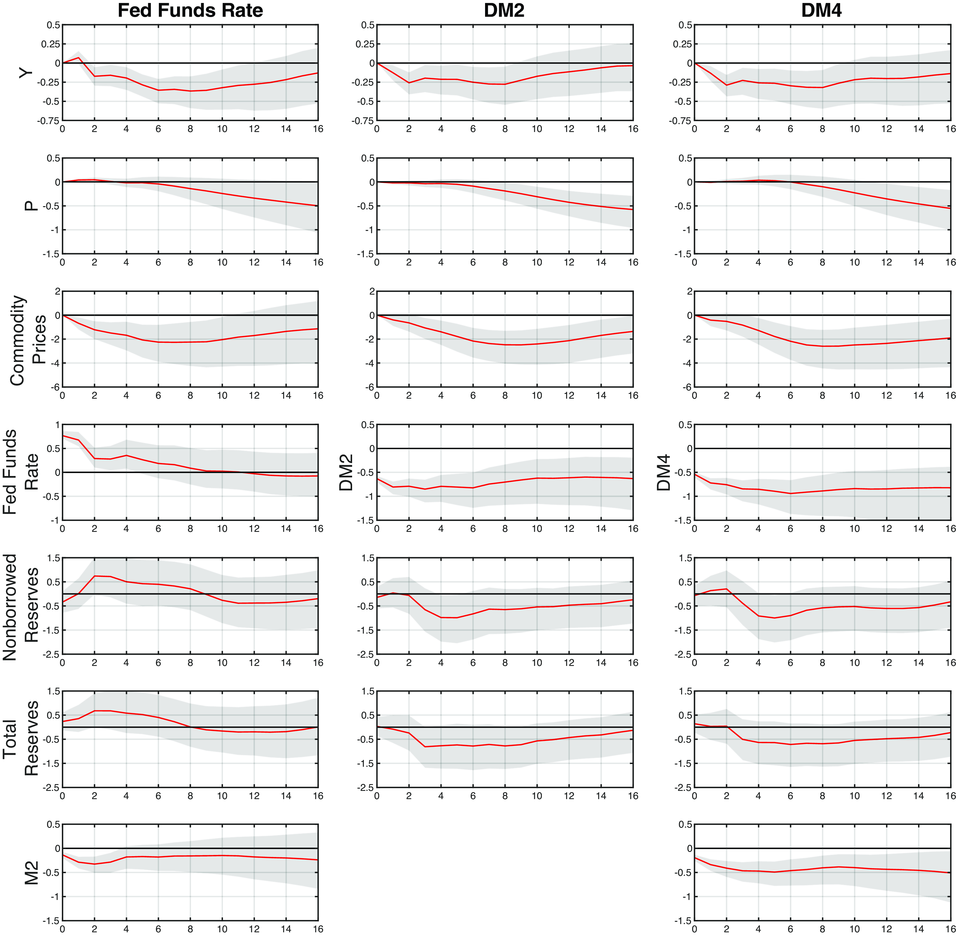
A monetary policy shock that raises the Fed Funds rate somewhat increases real GDP after one quarter, before having a negative impact from the second to the twelfth subsequent quarter. The initial positive impact contradicts conventional economic intuition and gives rise to an output puzzle. Moreover, a restrictive Fed Funds rate-based monetary policy shock also leads to a small increase in the price level for two quarters before turning to a negative impact, akin to the well-discussed price puzzle in the literature. However, the impact on prices is not precisely estimated.
A negative shock on either Divisia M2 or Divisia M4 for that sample yield fairly similar responses, which are the most informative and consistent with economic intuition. First, they both show a negative response of real GDP from 1 to 8 quarters after the shock. Second, both suggest that the impact on the price level is not significant in the first eight quarters, but becomes negative afterwards.
For a given monetary policy indicator $S_t$
, the impact is practically indistinguishable in sign, size, and significance on both nonborrowed reserves and total reserves. Their responses to a Fed Funds rate shock are positive in the second quarter. This differs somewhat from the responses of these variables to shocks on either DM2 or DM4, which are similar. However, the confidence intervals of both reserves’ responses to either monetary shock are mostly wide enough to include no impact, except for that second quarter in the case of a policy rate shock.
$S_t$
, the impact is practically indistinguishable in sign, size, and significance on both nonborrowed reserves and total reserves. Their responses to a Fed Funds rate shock are positive in the second quarter. This differs somewhat from the responses of these variables to shocks on either DM2 or DM4, which are similar. However, the confidence intervals of both reserves’ responses to either monetary shock are mostly wide enough to include no impact, except for that second quarter in the case of a policy rate shock.
Figure 7 refers to Keating et al.’s (Reference Keating, Kelly, Smith and Valcarcel2019) specification and ordering over the same period. The results are fairly similar to those obtained with Christiano et al.’s (Reference Christiano, Eichenbaum, Evans, Christiano, Eichenbaum and Evans1999), including the short-term output puzzle for the Fed Funds rate shock, while the negative response of real GDP to a restrictive Divisia monetary policy shock is less monotonous. Moreover, a slight one-quarter price puzzle occurs only with the Fed Funds rate shock.
Impulse response functions from 1967Q1 to 1995Q2 using Keating et al.’s (Reference Keating, Kelly, Smith and Valcarcel2019) ordering with different monetary policy signalling variables.
The name at the top of each column is that of the indicator variable used to construct the structural monetary policy shock.
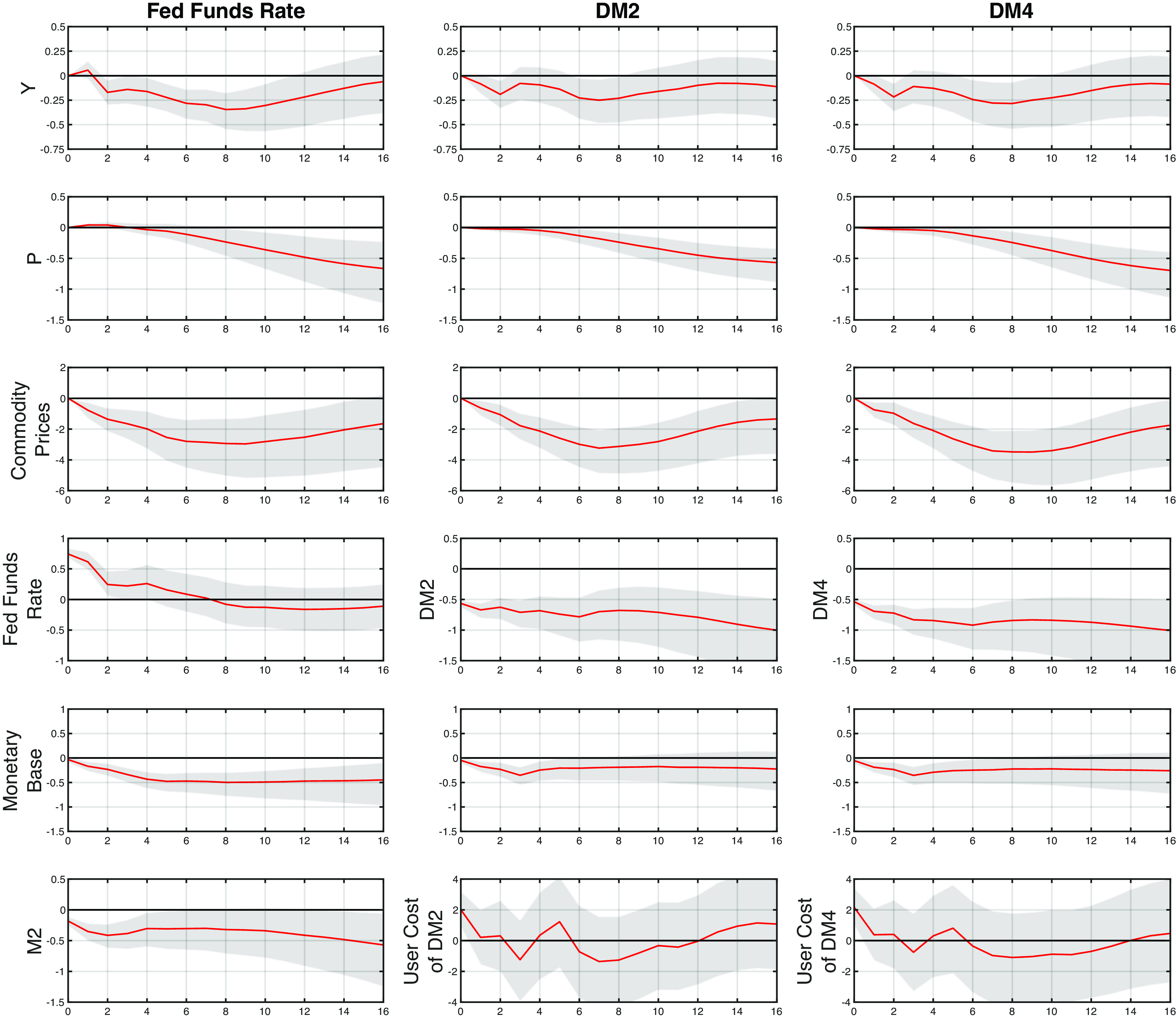
Before addressing whether the IRFs derived from constant-parameter VARs estimated are robust to the consideration of extended sample periods, we now check for the sensitivity of the 1967Q1–1995Q2 period’s results to the inclusion of additional variables in the empirical specifications.
First, we aim to evaluate how different structural shocks, derived from various monetary policy indicators, trace the impact of these shocks when the M2 or DM2 aggregate is included in the third block of the empirical specifications. Using Keating et al.’s (Reference Keating, Kelly, Smith and Valcarcel2019) identifying restrictions, the variables’ IRFs for the models with the Fed Funds rate, and DM4 can be visualized in Figure 8.
Impulse response functions from 1967Q1 to 1995Q2 using Keating et al.’s (Reference Keating, Kelly, Smith and Valcarcel2019) ordering with different monetary policy signalling variables and M2 vs. DM2 in the third block.
The name at the top of each column is that of the indicator variable used to construct the structural monetary policy shock. The impulse response functions and its corresponding 90% confidence band are shown for M2 (in blue) and DM2 (in red).

The overall appearance of the dynamic responses of real output to a given structural measure of the monetary policy shock is not very sensitive to the choice of adding either M2 or DM2 into the two models. In the model with the Fed Funds rate, the short-term output puzzle remains.
First, the overall appearance of the dynamic responses of real output to a given structural measure of the monetary policy shock is not very sensitive to the choice of adding either M2 or DM2 into both models. In the model with the Fed Funds rate, the short-term output puzzle remains. Additionally, having M2 does not subdue the price puzzle, and adding DM2 instead worsens it over that sample.Footnote 25 Also, with the inclusion of M2, the response of commodity prices to a Fed Funds rate shock remains significantly negative, but the negative response is weaker and not statistically significant when adding DM2. Most tellingly, the DM4 specification estimated for a sample closest to that of Christiano et al. (Reference Christiano, Eichenbaum, Evans, Christiano, Eichenbaum and Evans1999) that also includes either M2 or DM2 yields estimated responses that are quite similar in sign and size, with the direction of the effects being consistent with economic theory.
Second, as seen in the first column of Figure 9, adding DM4 to the Fed Funds shock model eliminates neither the short-term output puzzle nor the price puzzle. Rather, the price puzzle is reinforced. On the other hand, the second column in Figure 9 shows that adding the Fed Funds rate in the VAR’s first block, i.e., to the set of variables known by the Federal Reserve with no contemporaneous impact on DM4, yields no price puzzle following a DM4 monetary shock. However, following the monetary policy shock, there is a shorter-lived negative response of the Fed Funds rate that becomes insignificant after 4 or 5 quarters. Meanwhile, the specification with the Fed Funds rate in the model with DM4 also exhibits a counterintuitive positive response to a DM4 structural policy shock, albeit the overall response of real output remains statistically insignificant.
Impulse response functions from 1967Q1 to 1995Q2 from augmented models using Keating et al.’s (Reference Keating, Kelly, Smith and Valcarcel2019) ordering with different monetary policy signalling variables.
The name at the top of each column is that of the indicator variable used to construct the structural monetary policy shock. The impulse response functions and its corresponding 90% confidence band are shown without an additional variable (in blue) and with the additional variable (in red, where applicable).
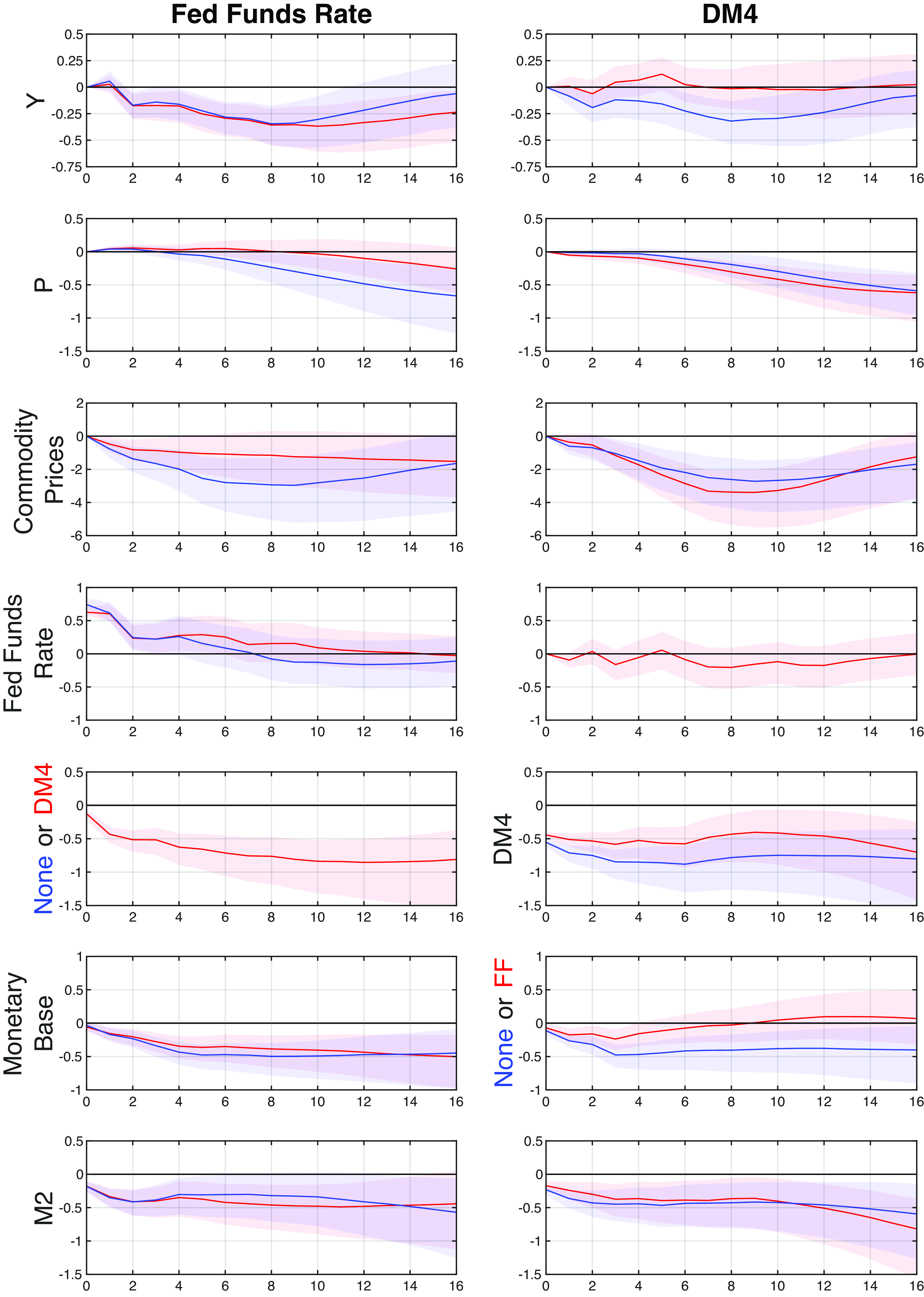
In summary, despite considering commodity prices and incorporating a Divisia index, the price puzzle stemming from monetary shocks based on the Fed Funds rate remains unsolved during the 1967Q1-1995Q2 period. Employing Keating et al.’s (Reference Keating, Kelly, Smith and Valcarcel2019) ordering, we will show in upcoming sections that with extended samples, the price puzzle persists across all samples when the monetary policy shock is derived from the policy rate, even with the inclusion of an appropriate money measure in an empirical model. Therefore, the reliance on the Fed Funds rate as the primary tool for assessing the monetary policy stance aimed at controlling inflation may have significant limitations.
5.2.2 The 1967Q1–2019Q4 period
We now turn to a longer sample, starting in 1967Q1 and ending in 2019Q4, before the COVID recession. Since this sample includes zero-lower-bound periods, we report the IRFs for the shadow-rate-based shock.Footnote 26
For all alternative monetary policy indicators, Figure 10 shows a negative response of real GDP to restrictive monetary policy shocks, which are fairly similar, except that the policy rate-based shock yields a short-term output puzzle. Moreover, there is clear evidence of a price puzzle following a positive shock on the policy rate, which raises prices. Following Christiano et al.’s (Reference Christiano, Eichenbaum, Evans, Christiano, Eichenbaum and Evans1999) suggestion and practice of including a commodity price index did not resolve the price puzzle and produced similar results to obtained when it was left out. This recommendation was motivated by the possibility that commodity prices might provide information about expected future inflation and might also be correlated with supply shocks, both being possible explanations for a price puzzle in a VAR that ignored these influences.Footnote 27
Impulse response functions from 1967Q1 to 2019Q4 with different monetary policy signalling variables.
The name at the top of each column is that of the indicator variable used to construct the structural monetary policy shock.
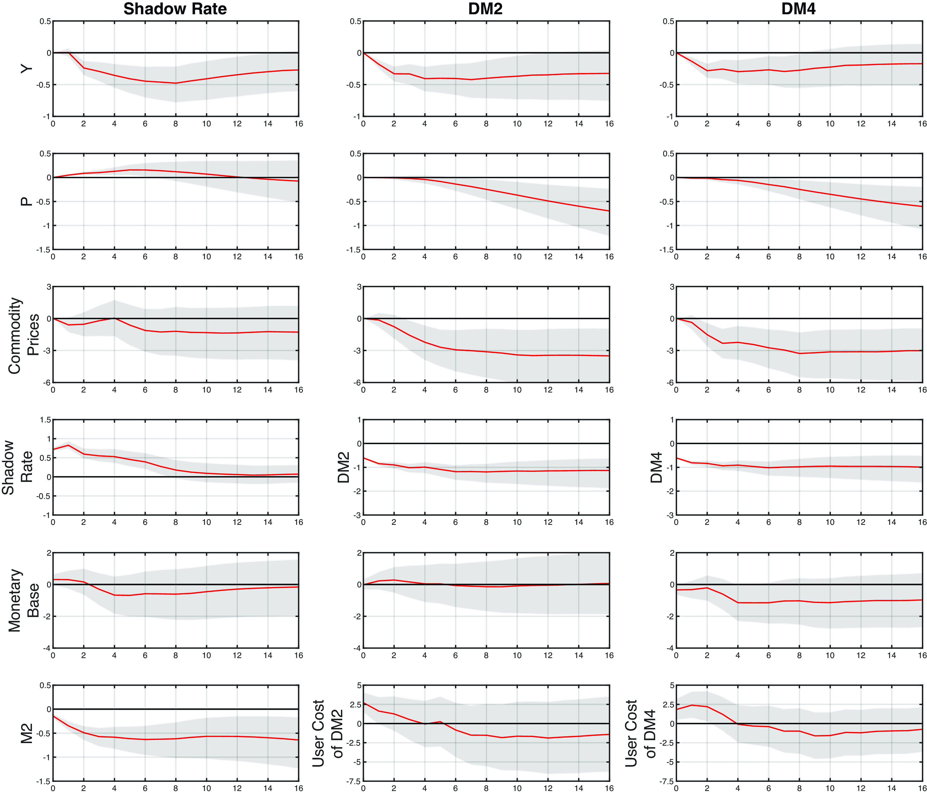
However, there is notably no statistically significant price puzzle when the signalling variable used to extract the shock is either DM2 or DM4 Divisia measures, with the negative impact on the price level occurring after four quarters or so. The lag in the manifestation of the theoretically expected effect on prices is also consistent with results found in the literature.
In particular, based on the evidence revealed by our SVAR with DM4 using data known in 2019, it is worth pointing out that if the US central bank had considered that DM4 would unexpectedly increase, as it did, either because of its actions and/or the working of the financial sector, the model would have strongly suggested that higher inflation was the likely outcome. A model that focused instead on the Fed Funds rate or the shadow rate would not have foreseen this.
Unsurprisingly, unexpected restrictive monetary policies with DM2- and DM4-based shocks are respectively associated with a 1- and 2-quarter rise in their own user cost.
5.2.3 The 1967Q1–2023Q4 period
At this stage, we extend the sample up to 2023Q4 to cover the COVID recession and the highly expansionary monetary policy that was pursued by the US central bank, followed by the beginning of some tightening. As done previously, when using the policy rate to represent monetary policy, we focus on the dynamic responses following a shadow-rate based shock in accordance with the zero-lower-bound spells within that sample.
Figure 11 shows the negative impact on real GDP of restrictive monetary policy shocks for all alternative indicators. However, when using the shadow rate, one quarter after the shock, real output is estimated to react positively, but not significantly. Overall, the negative response of output is clearer with the Divisia money aggregates.
Impulse response functions from 1967Q1 to 2023Q4 with different monetary policy signalling variables.
The name at the top of each column is that of the indicator variable used to construct the structural monetary policy shock.
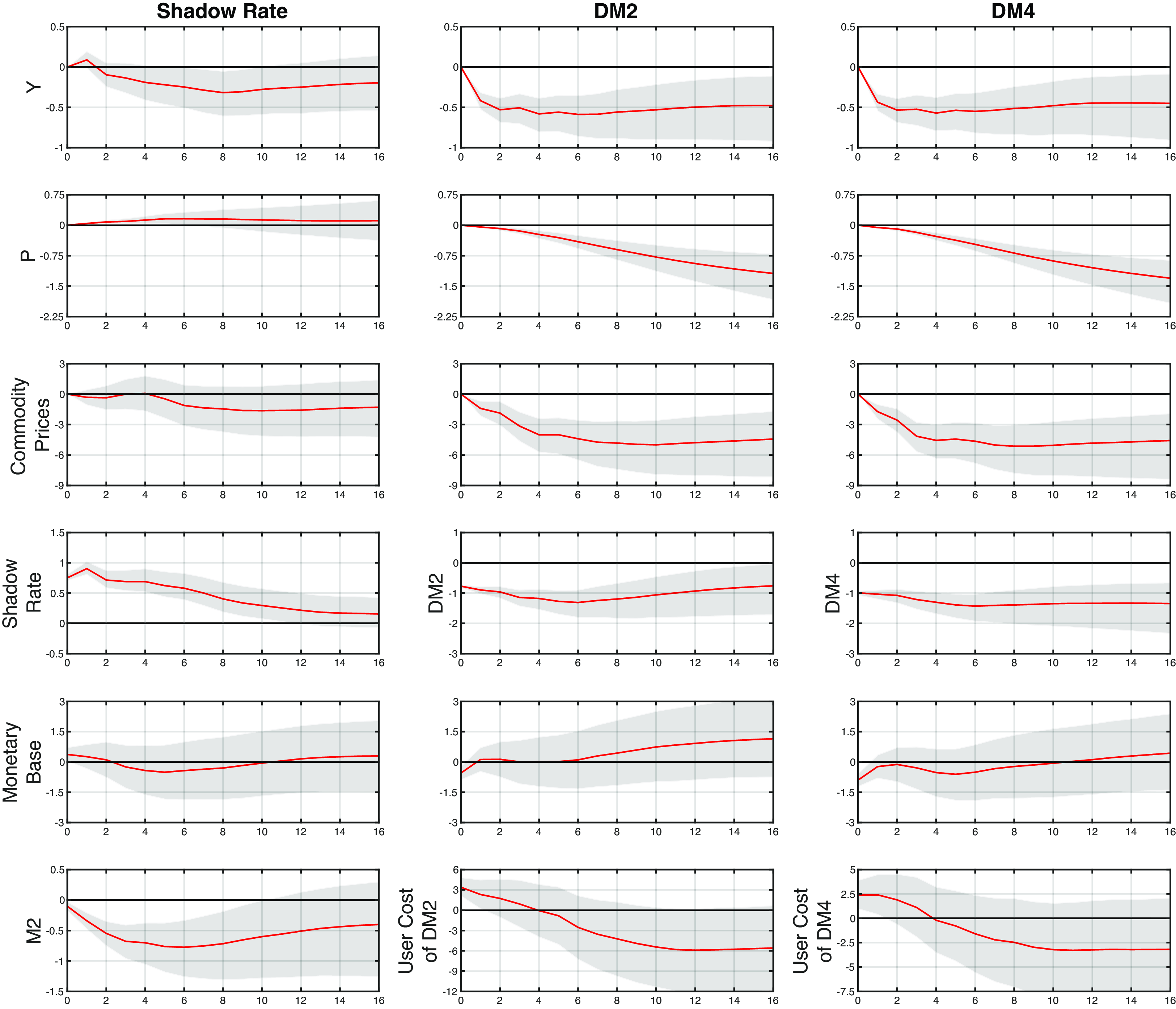
The price level’s response to a monetary policy shock inferred from the shadow rate still suffers from the price puzzle, even with the inclusion of commodity prices in the VAR. However, the impulse responses for the Divisia measures of money shocks do not exhibit a price puzzle, and the price level’s response builds steadily.Footnote 28
5.2.4 On the contribution of alternative monetary policy shocks to the variances of the variables
Another way to appreciate the evidence stemming from the different time-invariant VAR specifications is to highlight the contribution of each monetary policy indicator structural shock to the variances of key variables of the models at different horizons from 1- to 16- quarter ahead.
Figure 12 graphs results for 1967Q1-1995Q2 from the share of the variance of output, prices and the monetary base attributed to the Fed Funds rate as the monetary policy indicator, when M2 or DM2 is included in the VAR’s third block. Over that period, in the model with M2, the percentage of the variance of output attributed to the Fed Funds rate shock reaches its peak around the 9th quarter, with a contribution of about 15%, that of the monetary base is approximately 40% in the 9th quarter, and that of the price level reaches 15% after 16 quarters. However, if DM2 is included in the model’s third block, the contribution of the Fed Funds rate shock to both the variances of output and the monetary base increases as we extend the horizon, reaching about 35% after 16 quarters. Meanwhile, for that sample, the Fed Funds rate shock never accounts for more than 4% of the variance in prices for all horizons up to 16 quarters.
Contribution of fed funds rate monetary policy shock to the variance of Y, P and MB: 1967Q1–1995Q2.
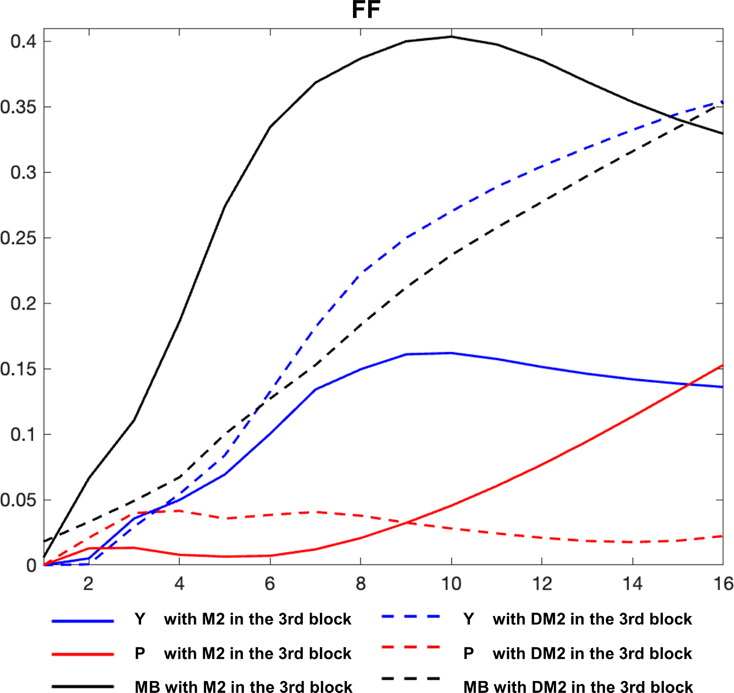
Figure 13 plots the contribution of alternative indicators of monetary policy shocks to the variances of output, prices and monetary base from the variance decomposition applied to both 1967Q1–1995Q2 and the 1967Q1–2023Q4. This figure illustrates quite clearly that while policy rate shocks fail to account for an important proportion of the variance of prices after 16 quarters, monetary policy shocks extracted from a Divisia monetary aggregate matter more. The Divisia monetary shock explains up to 23% of the price-level variance over the period from 1967Q1 to 1995Q2, and as much as 33% over the period that extends up to 2023Q4. With respect to the variance of output, the DM4 monetary policy shock contributes about 9% to its variance for 1967Q1–1995Q2, and nearly 13% for 1967Q1–2023Q4. However, the contribution of the monetary shock to the variance of the monetary base seems to be more sensitive to the sample period, which possibly reflects the use of quantitative easing, the payment of interest rates on banks’ reserves held at the Fed, and changes in the behavior of the demand for reserves after the Great Financial Crisis.
Contribution of alternative monetary policy shocks to the variance of Y, P and MB: 1967Q1–1995Q2 vs. 1967Q1–2023Q4.
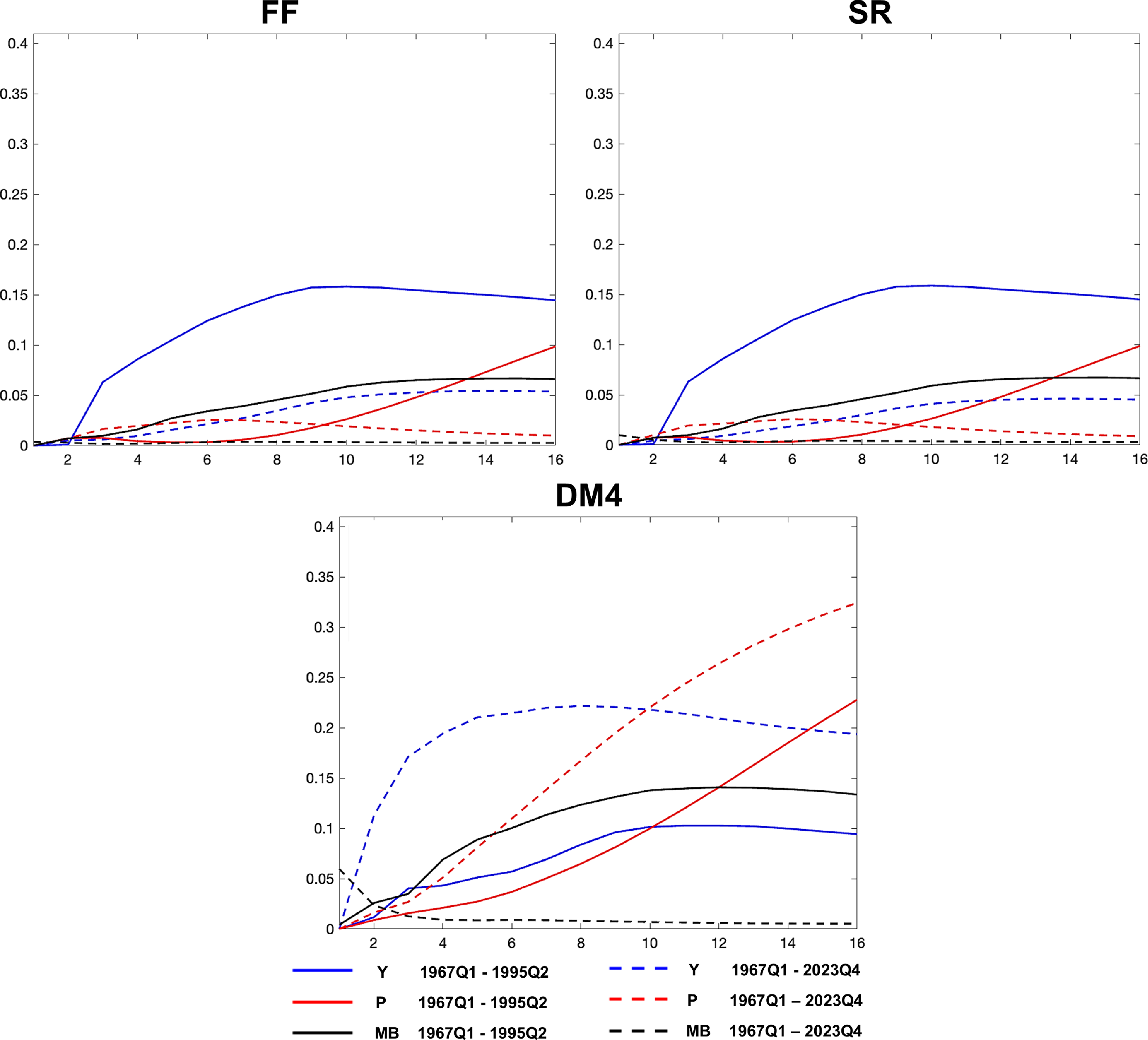
Apart from the checks discussed previously, the impulse response functions for the various time-invariant specifications were also generated across various subsamples and proved to show fairly stable shapes and patterns, with the DM4-inferred monetary policy shock being the most robust. The results were not altered in a substantive way, either when changing the number of lags or when proceeding with arguably reasonable changes in the identification ordering, such as increasing the information assumed to be known and used by the Fed when making its decisions (e.g., by moving $MB_t$
, or
$MB_t$
, or $MB_t$
and
$MB_t$
and $M2_t$
in the first block before
$M2_t$
in the first block before $S_t$
).Footnote
29
$S_t$
).Footnote
29
5.3. The out-of-sample forecast assessment of TVP-VAR specifications
The preceding section examined the results from estimating time-invariant VARs across various samples. However, the US economy has faced many changes since the late 1960s, including shifts in the Federal Reserve’s operating procedures and the real economy.Footnote 30 Accordingly, we now use recent advances in econometric methods to estimate time-varying parameter VARs and impulse response functions to monetary shocks based on alternative indicators of monetary policy. The variables included in the underlying time-varying specifications under consideration correspond to those used and associated with the first and third columns of Figure 11.
Before presenting and analyzing the results from time-varying IRFs, still keeping in mind the caveat made earlier regarding the crucial role of the identifying restrictions, it is nonetheless informative to review an assessment of the OOS forecasts of the different specifications of the TVP-VAR estimated with Goulet Coulombe’s (Reference Goulet Coulombe2025) 2-step-ridge-regression. Figure 14 displays the corresponding violin plots of relative RMSPEs whose shapes reflect the degree of accuracy in quarterly forecasting for the pseudo-OOS period from 2011 to 2023, and from 2020 to 2023.Footnote 31
Relative Root Mean Square Prediction Error (RMSPE) performance of pseudo-out-of-sample 1- to 8-quarters-ahead forecasts over 2011Q1–2023Q4 and 2020Q1–2023Q4 from 2SRR-TVP-VARs.
The vertical axis reports the ratio of the RMSPE from a particular forecasting model to the RMSPE from an AR(2), as the reference model, to compare the relative performance of alternative specifications. Seven specifications were considered. The label at the bottom of each violin shows the monetary indicator $S_t$
that was included. Moreover, in curly brackets, when applicable, it indicates whether M2
$S_t$
that was included. Moreover, in curly brackets, when applicable, it indicates whether M2 $_t$
or DM2
$_t$
or DM2 $_t$
was included within the third block of variables in addition to MB
$_t$
was included within the third block of variables in addition to MB $_t$
when the monetary indicator was either the Fed Funds rate or the shadow rate.
$_t$
when the monetary indicator was either the Fed Funds rate or the shadow rate.
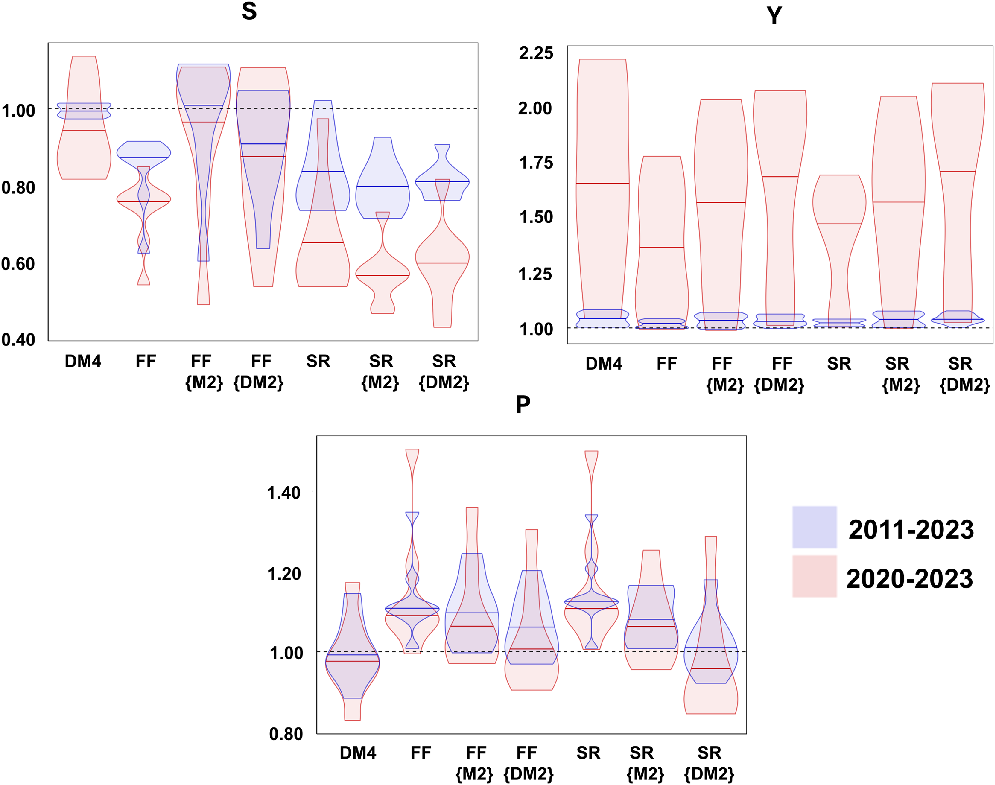
The forecasting performances of the TVP-VAR specifications are generally better than those of time-invariant ones, which raises the possibility that they are helpful in better capturing the underlying data-generating process and generating more reliable IRFs. Their ability to accurately forecast the monetary policy indicator is supported by empirical specifications built around either DM4 or SR{DM2}, which exhibit a lower median than the AR(2) benchmark forecasts. Moreover, although the violin plot for the DM4 specification suggests that its forecasting performance is more stable compared to that of the SR{DM2} specification, the height of the violin plot for the latter remains largely below one. However, all other specifications considered with the Fed Funds rate or the shadow rate were much more unstable in forecasting and, therefore, less reliable for predicting the policy rate. It is worth emphasizing that the relative ability to predict the evolution of the shadow rate in the SR{DM2} specification relies on the inclusion of the DM2 money aggregate.
With respect to the OOS forecasts for Y, the different models generate a fairly comparable degree of accuracy in terms of median and dispersion. However, the FF, FF{DM2} and SR{DM2} specifications reveal a slight advantage in forecasting real output over the DM4 specification.
Regarding the ability of the various models to forecast the price level, the DM4 specification shows the best RMSPE median performance with the least dispersion. The SR{DM2} specification does not perform poorly, but its median RMSPE is slightly higher and somewhat less stable.
Hence, the above analysis suggests that DM4 and its interactions with other variables in an empirical model provide relevant information about future price and output time paths.
Overall, our results are also in line with those in Clark and Ravazzolo (Reference Clark and Ravazzolo2015), who found that “extending the VAR-SV model to include time-varying parameters (VAR-TVP-SV) improves forecast accuracy in many, although not all, cases,” especially in point forecasting. As discussed in section 4.2 4.2.2, the 2SRR estimation proposed by Goulet Coulombe (Reference Goulet Coulombe2025) is proving to be a valuable alternative to the Bayesian TVP-VAR estimation with MCMC. Considering the forecasting quality of the 2SRR, it is expected that the IRF envelopes would more accurately capture the impact of the monetary policy shock stemming from the alternative variables compared to the IRF derived from the time-invariant VAR.Footnote 32 A by-product of the 2SRR estimation of the TVP-VAR is the estimation of a sequence of covariance matrices of the residuals for each quarterly observation. This, in turn, can be used, along with structural identifying restrictions, to estimate time-varying impulse response functions, which can be assembled as IRF envelopes and represented in 3D graphics.
5.4 Evidence from time-varying dynamic responses to alternative measures of monetary policy shocks over the 1967Q1–2023Q4 period
5.4.1 Motivation for the time-varying IRFs and their 2SRR estimations
In the next subsection, we produce and analyze the evolution over time of the IRFs for the different monetary policy signalling variables using 3D representations generated with 2SRR-TVP-VAR. Before doing so, we want to compare the IRFs calculated with three different estimators: the median IRFs obtained from TVP-BVAR; the estimates of the median IRFs obtained from the 2SRR-TVP-VAR; and the IRFs estimated from a fixed-coefficient VAR estimated over the whole sample. This allows us to evaluate the extent of the statistical significance of the estimates of the dynamic responses obtained from the 2SRR estimation.
Sections 4.2.2 and 4.2.3 discussed and compared the Bayesian estimator and the 2-step ridge regression estimator for TVP-VAR models. Both methods can be used to estimate variations in the dynamic responses of monetary policy shocks over the complete sample period from 1967Q1 to 2023Q4, except for the observations needed to accommodate the K-lags defining the order of the VAR. Thus, the effective estimation sample spans the 1967Q1+K to 2023Q4 period.
Yet, there are practical—and possibly not entirely innocuous—differences in how the two methods handle estimation and observations. Besides requiring the specification of priors for many hyperparameters and a burn-in phase for the simulation of MCMC draws, the TVP-BVAR method requires an initial training sample that excludes part of the data. This makes the TVP-BVAR estimates available for an even shorter sample and contingent on these earlier data. By comparison, over the whole effective sample, the 2SRR-TVP-VAR uses cross-validation techniques to tune the $K \times 1$
vector of time-smoothing parameters, which determine the extent of time variation needed in the VAR’s coefficients. Consequently, the 2SRR-TVP-VAR does not need an initial training sample that predates the production of our estimation and provides IRF estimates for all observations in the entire sample.
$K \times 1$
vector of time-smoothing parameters, which determine the extent of time variation needed in the VAR’s coefficients. Consequently, the 2SRR-TVP-VAR does not need an initial training sample that predates the production of our estimation and provides IRF estimates for all observations in the entire sample.
The production of our TVP-BVAR estimates is largely adapted to follow the procedure established by Primiceri (Reference Primiceri2005) and Giannone et al. (Reference Giannone, Lenza and Primiceri2015). First, because our model contains between 5 and 7 variables instead of 3 as in Primiceri (Reference Primiceri2005), it became difficult to obtain convergent estimates for a BVAR with a lag order higher than 2. That is why the comparison between the two estimators was set for TVP-VAR(2) models. Second, the number of burn-in samples was set to be in line with recent empirical papers, so 5 000 samples were discarded out of 20 000 draws in the MCMC. Third, for the models focusing on either the Fed Funds rate or the shadow rate as the indicator of monetary policy, the first 10 years (or 40 quarters) were used to calibrate and stabilize the prior distributions. However, we deemed it preferable to use 20 years (or 80 quarters) to stabilize the prior distributions for the models with the Divisia monetary aggregate as signalling variables, since their role has become more prevalent with the advent of quantitative easing in 2008. Additionally, we aimed to capture the COVID period’s potential effects, since unlike policy interest rates, which are limited by effective lower bounds, monetary aggregates are not subject to effective bounds. Fourth, the remaining hyperparameters of the priors were set to values similar to those recommended by Giannone et al. (Reference Giannone, Lenza and Primiceri2015) for a TVP-BVAR of this size.
Another point worth emphasizing in favor of the time-varying approach pertains to the treatment of the outlier in real GDP caused by the unprecedented COVID shock in the second quarter of 2020. Schorfheide and Song (Reference Schorfheide and Song2024) explain that the estimation of a time-invariant reduced-form VAR model is subject to severe distortions due to the extreme data points observed in that quarter, which deteriorate its forecasting ability. Consequently, unless one can “carefully” model the outliers by “inflating the scale of the measurement errors” or “inflating the scale of the state-transition innovations to capture innovation outliers,” they show that one option is to exclude the problematic observations. Our results indicate that the output outlier did not overtly influence our results, as the 2SRR-TVP estimation method ends up accounting for it.
We now proceed by comparing the median IRFs to a restrictive monetary shock obtained from three different estimators (VAR-OLS, TVP-BVAR, and 2SRR-TVP-VAR), using alternative indicator variables of monetary policy. For each median IRF, the shock at horizon 0 has been normalized to the OLS value for comparability.
Figure 15 shows the impulse response functions following a monetary shock, as observed through various indicator variables, over the periods 1967Q1–1995Q2 and 1967Q1–2023Q4, respectively. In each plot, the response generated for a constant-parameter VAR estimated by OLS is shown in red, along with its 90% confidence bands. The blue line represents the median response obtained by the Bayesian estimator of the TVP-VAR, with its 68% and 90% confidence bands shown in darker and lighter shades, respectively.Footnote 33 The green line is the median response estimated by 2SRR.
A comparison of median impulse response functions to a monetary shock with different monetary policy signalling variables for 3 different estimators.
The red lines show the IRFs and their corresponding 90% confidence bands estimated with a time-invariant VAR trained over 1967Q1-2023Q4. The blue lines depict the median IRFs from TVP-BVAR estimation and their corresponding 68% confidence bands for the Fed Funds rate shock over 1977Q1-2023Q4 and the DM4 shock over 1987Q1-2023Q4. The sample for the Bayesian estimation starts at a later date because of the training sample required to stabilize the priors’ distributions, but ends in 2023Q4. The green lines are the median IRFs for 1967Q1-2023Q4, but obtained from 2SRR-TVP-VAR estimations for 1967Q1-2023Q4.
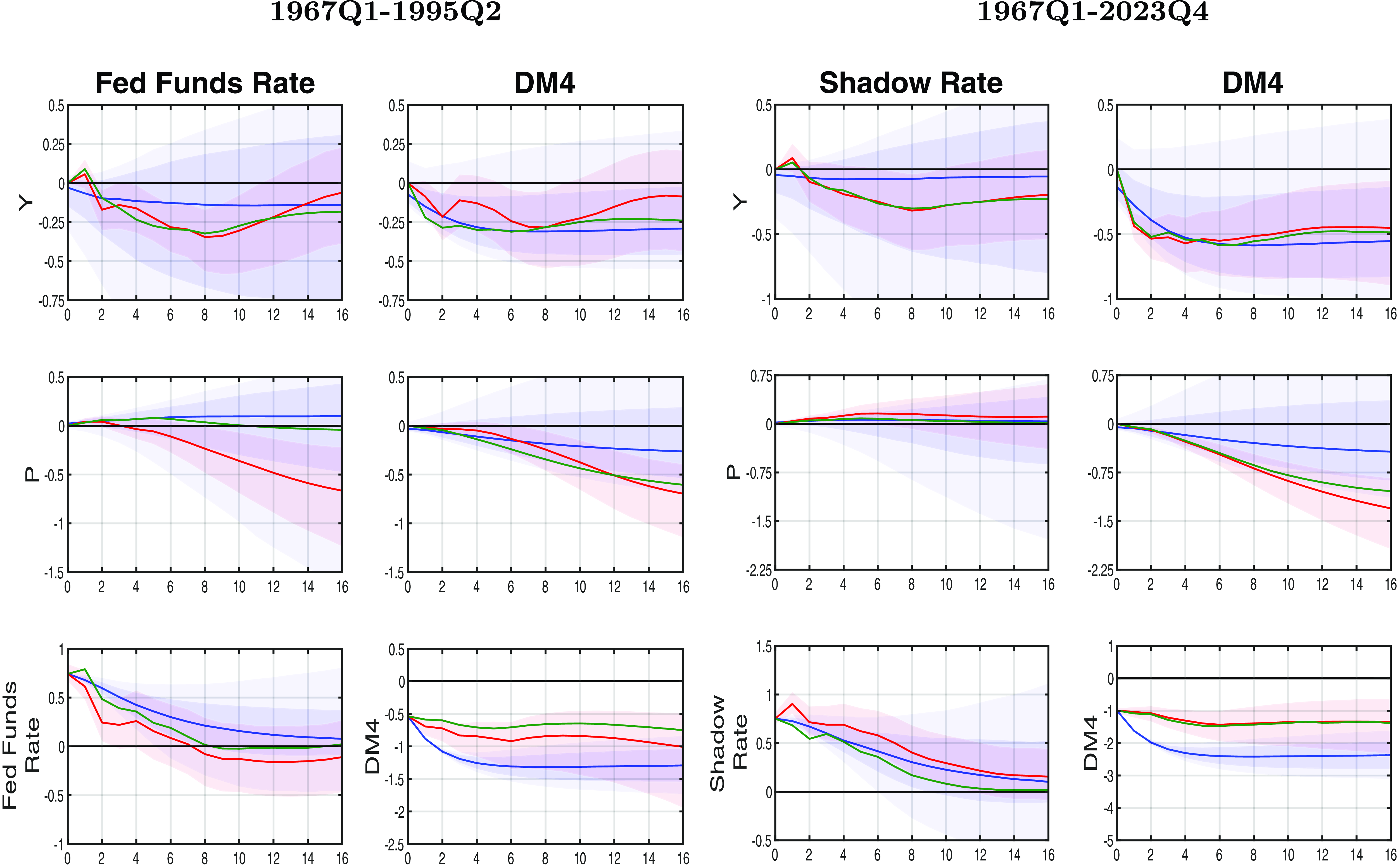
Unlike time-invariant OLS VAR models, which rely only on data from the selected sample period, time-varying models use the entire dataset to provide a more accurate estimate of the underlying process. This comprehensive approach allows these models to better capture the dynamics of the process during specific subsample years. By incorporating information from the entire time span, time-varying models can reveal relationships between variables that may not be apparent when using only a limited dataset. As a result, the response of certain variables may differ significantly from that observed in an OLS model, especially if the initial data were insufficient to fully capture the underlying relationships. Conversely, if the responses are similar to those obtained from the OLS model, it suggests that the median relationship between variables has remained relatively stable over the years. Still, this does not preclude some variation over time, which underscores the importance of considering time-varying models for a more nuanced understanding of economic dynamics.
As seen in the first two columns of Figure 15, for the 1967Q1–1995Q2 period, the estimated dynamics of the monetary indicator following a policy shock on the central bank’s interest rate are analogous for the three estimators, and the confidence bands for both the OLS and Bayesian estimators mostly overlap. On the other hand, the median negative impact of the monetary aggregate shock on DM4, based on the Bayesian estimator, appears to be somewhat stronger than that for the 2SRR estimator. The latter is also quite similar to the response obtained with the OLS estimate for a constant-parameter VAR.
By and large, the responses of GDP and the price level are quite similar across estimators. The exception is the OLS-based IRF for prices after a Fed Funds rate shock, which may be stronger from the 8th quarter onward. Also, the Bayesian-estimator-based IRF for prices is a little stronger than that of the 2SRR. In any case, the median response of prices suggests a possible price puzzle with the Fed Funds rate model, which is not the case for the DM4 model.
Extending the comparison of the three estimators to the 1967Q1–2023Q4 period, the IRFs for the three estimators displayed in the last two columns of Figure 15 are broadly consistent with those for the earlier period. In particular, the median price response to a shadow-rate-based monetary shock is affected by the price puzzle. However, there is no price puzzle in the median responses to the broad Divisia monetary aggregate-based shocks, and the patterns of these responses are consistent with both the TVP-BVAR and the 2SRR-TVP-VAR estimates.
Finally, the confidence intervals of IRFs from the time-invariant VAR, TVP-BVAR estimations, and the point estimate variations depicted in Figure 15 imply the statistical significance of the 2SRR-TVP-VAR estimates.
5.4.2 The estimated time-varying cumulative IRFs
The advantages of estimating time-varying parameter VARs and their corresponding time-varying IRFs lie in their ability to capture how the size of monetary policy shocks has fluctuated and how responses to these shocks may have shifted over time. To this end, we find 3D representations of the cumulative IRFs, which amount to envelopes of the IRFs, to be best suited for assessing the extent of time variation. We find this approach even more revealing than the conventional representation of the median of the time-varying responses often reported in TVP-VAR.
With a time-invariant model, the size of the initial monetary policy shock is imposed as being constant. However, in a TVP model, the size of the initial policy shock varies over time by design, reflecting the evolving nature of the system. The estimated initial shock over time provides valuable insights into the evolution of these shocks across different periods. For each alternative monetary policy signalling variable, Figure 16 plots the unscaled estimated initial (restrictive) monetary policy shocks over the 1968Q1–2023Q4 sample. Although these are not the model’s predictions or fitted values, the plotted values represent the magnitude of the initial shock’s impact on the indicator variable. Moreover, as in the time-invariant models, the impact of shocks is symmetric. Thus, a positive value represents the intensity of a restrictive initial policy rate shock, while a negative value indicates the intensity of a restrictive initial Divisia monetary aggregate shock (and vice versa). For example, if the immediate response of the policy interest rate to structural monetary policy shocks has increased, monetary policy may have acted more swiftly in response to economic conditions or adopted a more proactive stance.
Unscaled estimated initial (restrictive) monetary policy shocks for alternative monetary policy signalling variables over the 1968Q1–2023Q4 sample.

Figure 16 suggests different interpretations of monetary policy actions based on shocks to the policy rate versus to the Divisia monetary aggregates. The absolute size of policy rate shocks indicates that monetary policy sent a stronger signal towards tightening in the late 1970s and early 1980s than it did towards the loosening of policy during the Great Recession and the COVID pandemic. However, shocks from the Divisia monetary aggregate show similar policy shock sizes between 1968 and the early 2000s, with a much larger expansionary shock during the pandemic.
Because the size of the variance of the shocks has itself varied over time, we now present and discuss the 3D time-varying IRFs for the standardized estimated structural shocks. Figures 17 to 19 show scaled 3D representations of the point estimates for time-varying impulse response functions of key variables in our alternative models after a one-unit monetary policy shock.Footnote 34
Cumulative IRF envelopes for the monetary policy indicator following a restrictive monetary policy shock over 1967Q1–2023Q4.
Interactive 3D representations are available at (a) https://sites.google.com/view/barrettepaquet2025/effective-federal-funds-rate/on-itself, (b) https://sites.google.com/view/barrettepaquet2025/shadow-rate-wu-xia-2016/on-itself, (c) https://sites.google.com/view/barrettepaquet2025/divisia-m4/on-itself.
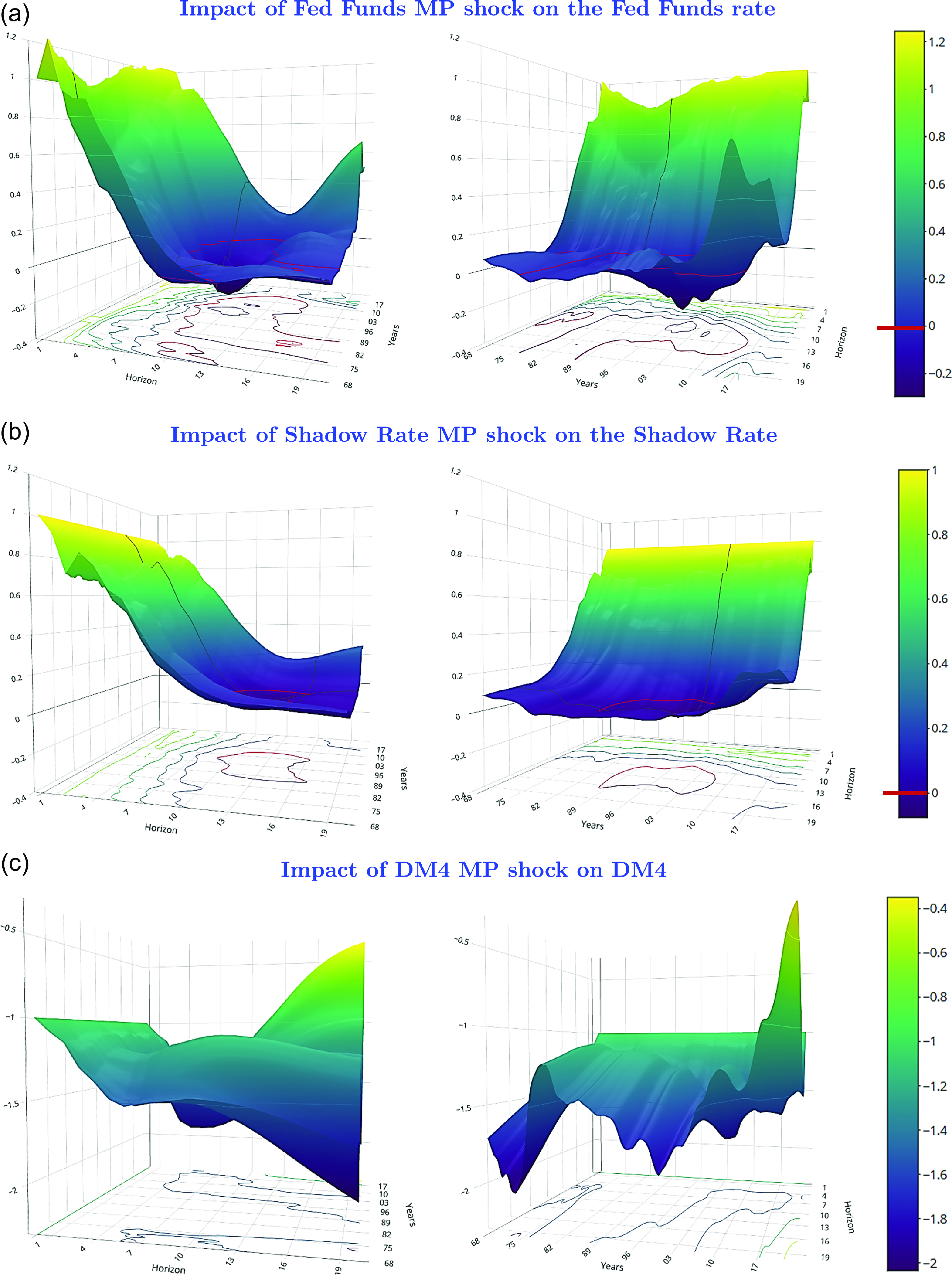
Cumulative IRF envelopes for real GDP following a monetary policy shock over 1967Q1–2023Q4.
Interactive 3D representations are available at (a) https://sites.google.com/view/barrettepaquet2025/effective-federal-funds-rate/on-gdp, (b) https://sites.google.com/view/barrettepaquet2025/shadow-rate-wu-xia-2016/on-gdp, (c) https://sites.google.com/view/barrettepaquet2025/divisia-m4/on-gdp.
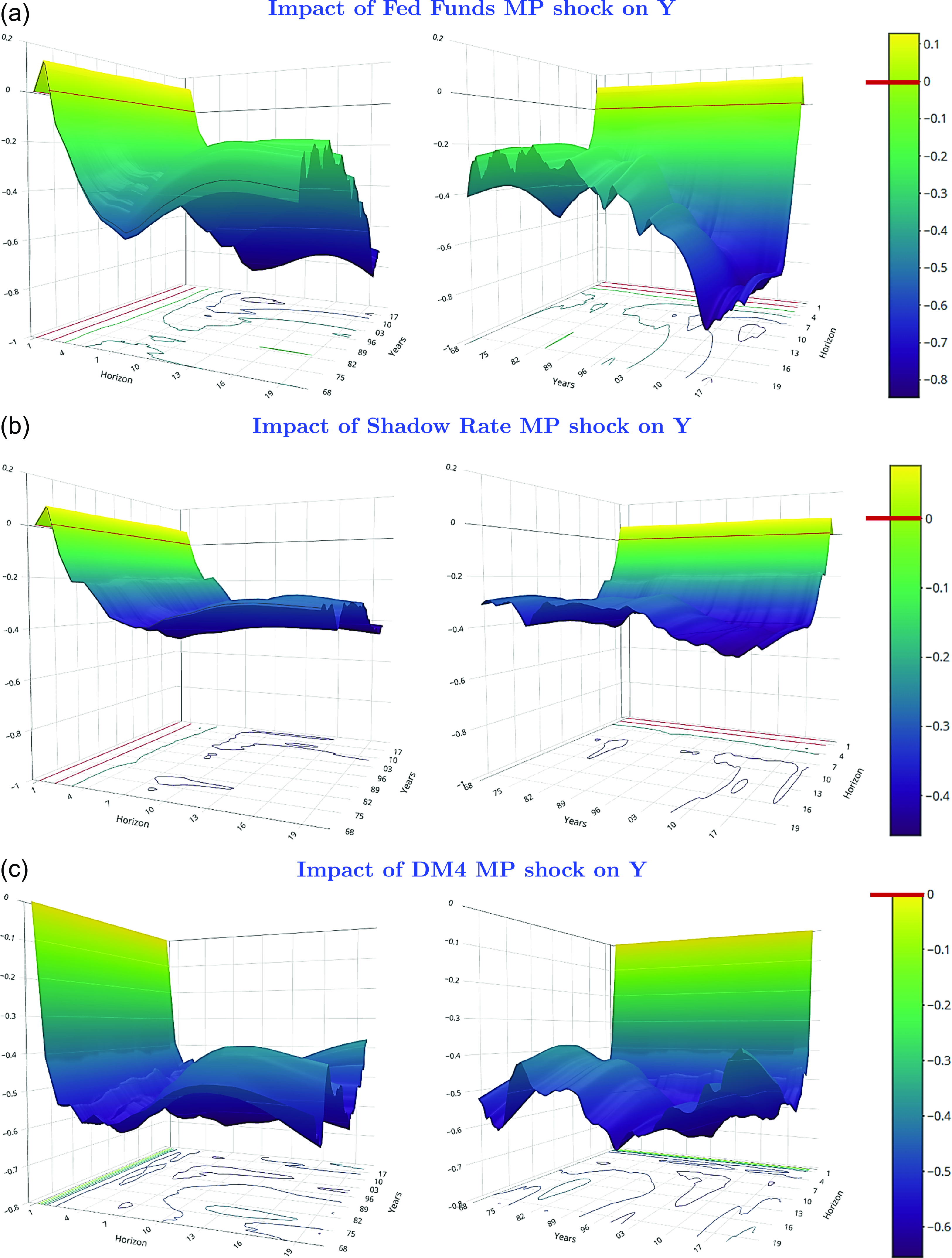
Cumulative IRF envelopes for the price level following a restrictive monetary policy shock over 1967Q1–2023Q4.
Interactive 3D representations are available at (a) https://sites.google.com/view/barrettepaquet2025/effective-federal-funds-rate/on-prices, (b) https://sites.google.com/view/barrettepaquet2025/shadow-rate-wu-xia-2016/on-prices, (c) https://sites.google.com/view/barrettepaquet2025/divisia-m4/on-prices.
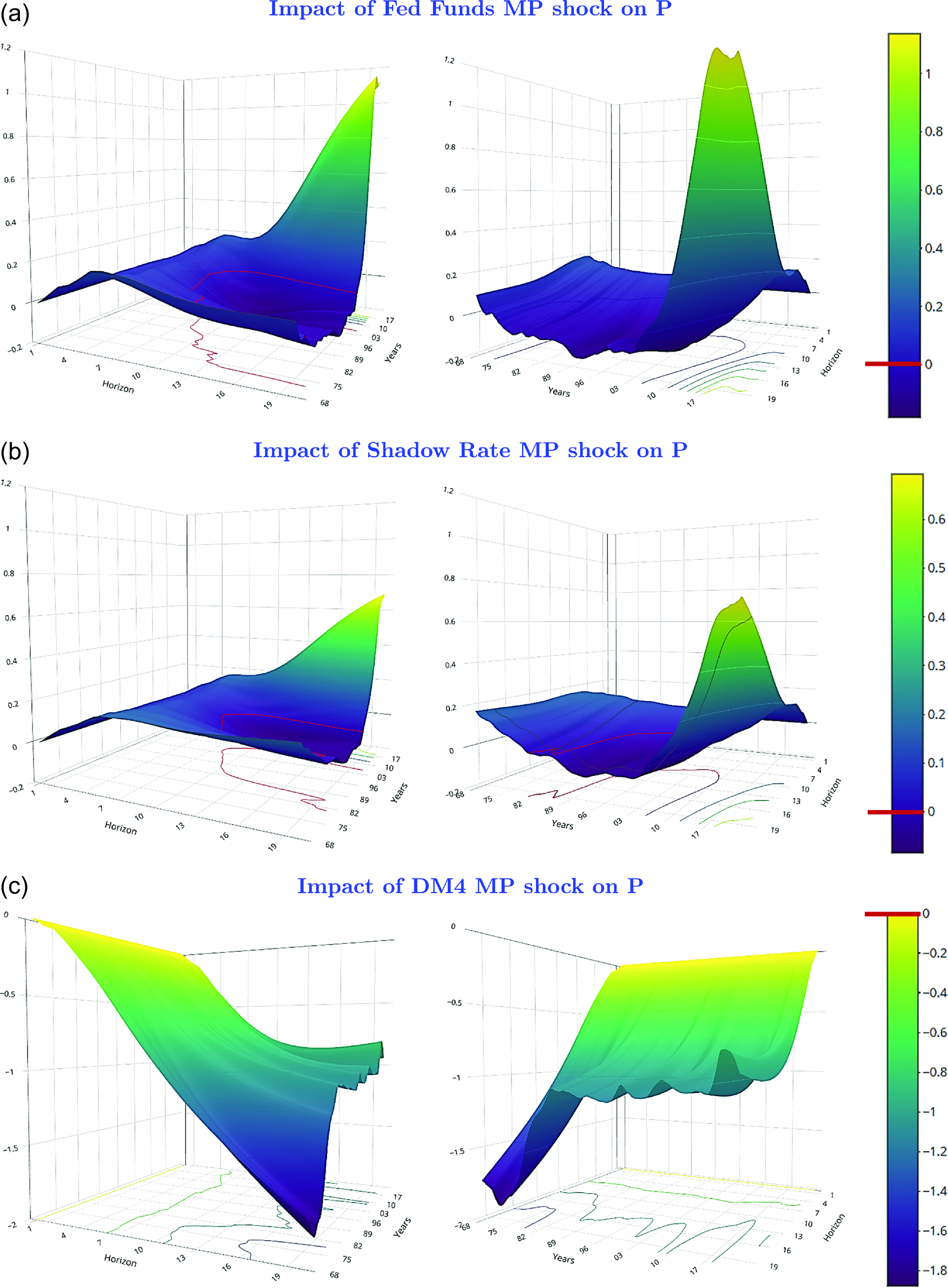
According to Figure 17, a restrictive monetary policy shock in period 0 causes an immediate rise in the Fed Funds rate or shadow rate, or a decrease in DM4, depending on the specified policy indicator. In particular, the cumulative impact on DM4 following its own initial shock has gained importance over the observations preceding the early 1980s. By contrast, since 2017, the cumulative impact of a restrictive monetary policy shock on DM4 has been relatively mitigated. In the DM4 specification, a one-unit shock on the broad Divisia money aggregate is followed by a somewhat persistent decrease in its level. Moreover, the impacts are not monotonic, and the size of the variations in this broad Divisia aggregate has not been constant over the whole sample.
The variation over time in the size of the response to a monetary policy shock is not surprising. For one thing, a DM4-monetary policy shock has likely induced different implicit impacts on the components making up the aggregates. Moreover, this monetary policy shock has possibly implicitly impacted the weights of each component. Although this cannot be verified in our model, as it does not separately include all the assets that compose Divisia M4, the dynamics specific to the broad aggregate should be consistent with our conjecture.
Figure 18 illustrates the response of real GDP to a one-unit monetary shock for the three alternative measures. In agreement with economic intuition, in the presence of short-term nominal rigidities in prices and/or wages and because of liquidity effects, the FF and SR specifications imply that a restrictive monetary policy is followed by a decrease in aggregate real output, at least from the second quarter on. The positive impact in the quarter that immediately follows the shock is counterintuitive, albeit it may be deemed small.
For both the FF- and SR-based monetary policy shock, the largest drop in real GDP is reached 8 or 9 quarters after the shock, before the impact starts subsiding. With a one-unit restrictive FF-based monetary policy shock, the biggest reduction in output remains fairly constant until the early 1990s. However, afterwards, the largest trough deepened even more until the end of our sample. A similar phenomenon is documented for the SR-based monetary policy shock. After 20 quarters, a negative effect still remains, with the time variation of the corresponding point estimates staying within the same range. However, at the turn of the century, despite a jump in the FF-based shock time-varying IRFs around 2007, both policy rate shocks indicate that the IRFs for real GDP have faced subsidence. Consequently, in 2022, this translates to the FF-shock having an impact estimated to be 2.8 times larger after 20 quarters than it was in 2000. For the SR-shock, over the same horizon, the impact is now about 68% above what it used to be.
When a restrictive monetary policy shock is extracted using DM4 as the signalling variable, the negative responses of real output align with economic intuition. Unlike the shock on the policy rate, there is no objectionable positive effect in the first quarter. The largest impact occurs between 6 and 8 quarters, followed by some catching up. With a DM4-based restrictive monetary policy shock, the corresponding IRF envelope for real GDP shows a steep drop during the 5 to 6 quarters following the shock, while remaining fairly stable over time. The strongest impact is slightly deeper at the trough, but the subsequent recovery has been less uniform. Our estimation also suggests that the speed of recovery after a negative monetary shock gathered momentum over time, especially from 2012 to 2016. Despite moderate fluctuations in the shape of the IRF envelope, it remains fairly high from 2016 to 2022. This is consistent with casual observations of economic activity dynamics.
The propagation of a one-unit monetary policy shock on prices for each specification is displayed in Figure 19. Examining these 3D graphics is quite enlightening.
Figure 19 shows a striking price puzzle when measuring monetary policy shocks in a TVP-VAR model with the Fed Funds rate or shadow rate. A restrictive shock to the Fed Funds rate leads to an anomalous price increase for at least 8 quarters throughout the entire period, worsening since the early 2000s. The shadow-rate-based shock shows a less strong but still prevalent price puzzle 20 quarters after the shock, except from 1988 to the early 2000s when price responses turned mildly negative. These responses are particularly confounding after the mid-1990s due to the Fed’s adoption of inflation targeting and the anchoring of trend inflation expectations, at least until the latest bout of higher inflation.Footnote 35
Thus, for both policy rate measures, the price puzzle often persists for up to 20 quarters. For the federal funds rate shock, it lasted from 1968 to 1974, while for the shadow rate shock, it continued until around 1980. Subsequently, the duration of the price puzzle following a policy rate shock was typically less than 8 quarters until around 2007. However, it became more pronounced afterwards, extending beyond 20 quarters.Footnote 36 This indicates that pre-1975 information remains relevant for adequately extracting and assessing the implications of a structural monetary shock and its impact using TVP-VAR models as well.
However, the literature has largely omitted that period, either because it was considered a “different time” for monetary policy or because the Bayesian econometric method used to estimate the TVP-VAR required an initial training sample, resulting in its exclusion from the estimation sample. By utilizing the complete dataset and integrating the latest data up to 2023, the 2SRR estimator applied to a TVP-VAR offers a more accurate representation of the price puzzle associated with an assumed policy rate-based monetary shock.
Contrary to the evidence for a shadow rate shock, the time-varying dynamic responses in Figure 19, produced with monetary policy shocks identified using DM4 as the indicator variable, are not affected by the price puzzle and exhibit similar patterns throughout the entire sample. For every quarter from 1968 to 2022, a one-unit restrictive monetary policy shock is followed by a gradual decrease in the price level, in accordance with economic theory.
According to the DM4 specification, it is observed that up to about 10 quarters after the shift in monetary policy stance, the effects on prices are similar throughout the entire sample. From 10 to 20 quarters after the shock, a one-unit restrictive monetary policy shock continues to push the price level down. However, from the early 1990s until 2017, the response of prices to a DM4 monetary policy shock tended to stabilize at a lower level. Since then, a negative shock on DM4 still has a negative impact on prices, but the price level does not decrease as much after 20 quarters than after 13 quarters. The overall shape of the price responses to a DM4-based monetary shock is particularly consistent throughout the entire sample. Given the consistent overall shape of the envelope of the IRFs, even in the midst of the COVID episode, our results are not sensitive to extreme values of real GDP in the second quarter of 2020.
6. Conclusion
Using data from 1967 onward (extended to include the post-pandemic inflationary episode), we applied traditional and new econometric methods to analyze the informational relevance of Divisia money for extracting monetary policy shocks and assessing their transmission, compared with alternative indicators. This provides valuable empirical lessons that reinforce the importance of money in monetary policy.
The evaluation of Divisia measures confirms their usefulness and highlights the superiority of empirical models that include them in studying monetary policy transmission. Our findings indicate that interest rates alone fail to produce dynamic responses consistent with expected intuition or free from empirical puzzles, especially for samples extending past the early 2000s and the recent inflation resurgence. In contrast, Divisia monetary aggregates, which are theoretically superior to simple-sum measures, generate puzzle-free and economically reasonable IRFs for both output and prices. These results align with previous studies, including Keating et al. (Reference Keating, Kelly, Smith and Valcarcel2019) and Chen and Valcarcel (Reference Chen and Valcarcel2021), who used different estimators and periods. We also find that output and prices respond more significantly and quickly to monetary policy shocks when Divisia measures are used compared to other indicators. Overall, a deeper understanding of the role of monetary aggregates in monetary policy impact is essential.
Our results do not imply that the policy rate is irrelevant or lacks a role in influencing output and prices. Forward guidance and news effects are still likely to matter. However, ignoring the information content and the central bank’s transmission of Divisia money can be hazardous. For instance, even with the Fed Funds rate being the favorite instrument, overlooking the growth rate of Divisia money while focusing heavily on interest rate shifts and output gap measurements could lead to policy rate overshooting, which might unduly harm real output.
Rethinking and clearly defining the role of monetary aggregates in policy could be crucial. Our empirical results, coupled with the recent surge in inflation and the slightly lagging return of its core value to the 2% target, highlight the importance of not ignoring money. Therefore, it’s essential to better define the role of a Divisia broad monetary aggregate, whether as an indicator or an intermediate target, and to precisely determine its relationship with operating targets.
In the debate among policymakers and in the financial press about fighting inflation, it was argued that monetary policy has been historically restrictive, given the Federal Reserve’s 525 basis point increase in the Fed Funds rate over 11 meetings between March 17, 2022, and July 26, 2023. Despite this, with core inflation still above 4% in fall 2022, it is unclear if a nominal Fed Funds rate of 3% to 4% was truly restrictive, as the real rate remained negative or barely positive for much of 2022. The early rate hikes likely signaled the central bank’s commitment to controlling inflation. Yet, a closer look at the growth rate of Divisia M4 would have shown its slowdown starting in 2021, intensifying in spring 2022, which may partly explain the decrease in inflation in late 2023 and the first half of 2024. This is consistent with the P-star model analysis by Hallman et al. (Reference Hallman, Porter and Small1991) and recent studies by Ireland (Reference Ireland2023, Reference Ireland2025).
The robustness of the results regarding the relevance of Divisia money has significant implications for policymakers and researchers, paving the way for future studies. Subsequent work could extend the analysis to other countries with accessible Divisia data (e.g., Barnett et al. Reference Barnett, Ghosh and Adil2022). Given that recent QE policies were accompanied by substantial government programs, including fiscal policy variables in the model could shed light on the interaction between fiscal and monetary policy shocks. This could involve adding variables related to government consumption expenditures, transfers, and public investments, or considering the public debt/GDP or deficit/GDP ratios. Empirically, it might be insightful to explore the asymmetric effects of monetary shocks derived from Divisia money aggregates. In addition, both theoretically and empirically, constructing and analyzing monetary multipliers or detailing the financial mechanisms behind the creation of inside money tied to Divisia measures could enhance our understanding of monetary policy transmission.
Acknowledgements
Forthcoming in the special issue of Macroeconomic Dynamics entitled “Divisia Monetary Aggregates and the Macroeconomy”
We are grateful to the Special issue Editor and two anonymous referees for comments that greatly improved the paper, to John Keating and Philippe Goulet Coulombe for helpful discussions, as well as to Sergio Lago Alves, Steven Ambler, Bill Barnett, Olivier Coibion, Paul Hubert, Dalibor Stevanovic, and participants at the 2023 Canadian Economic Association Meetings and Congrès de la Société canadienne de science économique, at the Brown Bag Workshop for Macro Research in Montreal, at the 2024 Annual Conference of the Society for Economic Measurement, as well as in seminars at the Banque de France, at Kansas University, and at the Observatoire français des conjonctures économiques for comments on earlier versions. The usual caveat applies.
Competing interests
The authors declare none.


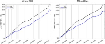


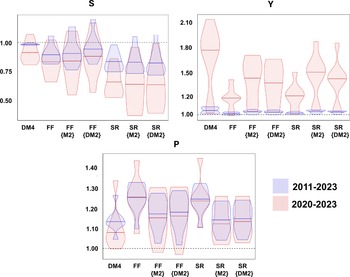


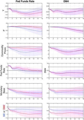


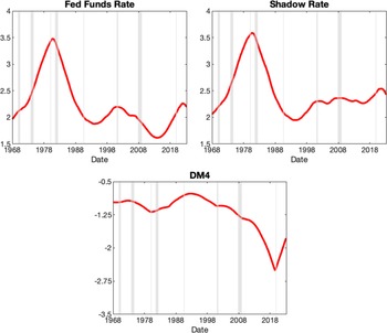
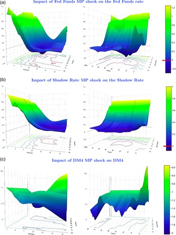


 Open access

