





Impact statement
BLI propulsion is a promising route towards more energy-efficient and lower-emission aircraft, yet its practical implementation is strongly limited by inlet distortion and the associated fan stability issues. This work combines URANS and LES in a full-annulus intake–fan configuration to reveal how distorted inflow organises into a persistent distorted sector at the AIP and how this sector controls rotor incidence, hub-corner separation and loss generation in the stator passages. The study identifies a sector-fixed loss pattern and clarifies the role of fragmented vortex systems in driving throughflow decay. These insights provide a physics-based basis for defining critical sectors, monitoring indicators and design margins in BLI fan applications, and they are relevant to a broad class of intake–fan integrated systems operating under non-uniform inflow conditions.
1. Introduction
Boundary layer ingestion (BLI) propulsion is widely recognised as a promising pathway for reducing noise, emissions and fuel burn (Liu et al. Reference Huang, Lin, Tan, Bai, Jia, Zhu and Liu2024; Ma et al. Reference Ma, Lu and Li2025). When a fuselage boundary-layer fluid is ingested by a fan and accelerated, wake losses are reduced and airframe drag is further lowered. This is often termed the ‘BLI benefit’ (Farokhi Reference Farokhi2019; Hall et al. Reference Hall, Huang, Uranga, Greitzer, Drela and Sato2017). Recent studies have shown that, relative to conventional configurations, BLI can deliver substantial reductions in fuel consumption while improving propulsive efficiency across multiple aircraft concepts (Harouni Reference Harouni2014; Moirou et al. Reference Moirou, Sanders and Laskaridis2023). However, a fan must then operate under highly distorted inlet conditions that can cause unsteady rotating instabilities, severe aerodynamic noise and potential non-synchronous vibration (Hefang et al. Reference Hefang, Zhang, Kailong, Qiang, Mingmin and Jinfang2025). Consequently, the rigorous characterisation of the inlet distortion induced by fuselage boundary-layer ingestion is a prerequisite for ensuring the safety and reliability of BLI propulsion systems.
Previous studies (Gong, & Yuan Reference Gong and Yuan2021; Lucas et al. Reference Lucas, O’Brien and Ferrar2014; Rademakers et al. Reference Rademakers, Stößel, Kožulović and Niehuis2025) have indicated that, relative to uniform inflow, BLI-induced distortion not only increases aerodynamic losses and degrades propulsive performance, but also markedly alters an engine’s internal flow topology, thereby intensifying aerodynamic interference and interstage coupling. From a structural perspective, distorted conditions impose cyclic loading and unloading on the blades, which substantially elevate the fatigue loads and shorten the service life (Provenza et al. Reference Provenza, Duffy and Bakhle2019). Aerodynamically, the distortion modifies the incidence at the rotor inlet and increases flow losses. With the alteration of the rotor outlet flow angle, the distortion further exacerbates stator losses (Gunn et al. Reference Gunn, Tooze, Hall and Colin2013). Consequently, the distortion-induced degradation of fan aerodynamic performance erodes the inherent aerodynamic advantages of BLI, which underscores the urgent need for high-performance, distortion-tolerant fan designs.
Against this backdrop, the accurate resolution of the unsteady flow characteristics and loss mechanisms with BLI-induced distortion is a central issue at the fan design stage (Pan et al. Reference Pan, Shi, Lu, Yang, Zhang and Li2024). Mårtensson & Billson (Reference Mårtensson and Billson2024) indicated that BLI fans exhibited pronounced distortion over the low-speed operating range from subsonic to transonic conditions, and the resulting total-pressure distortion induced complex unsteady aerodynamic responses. Computational fluid dynamics has been widely employed to explain the underlying mechanisms, particularly steady full annulus Reynolds-averaged Navier–Stokes (RANS) simulations, which have been used to capture boundary layer ingestion, wake interactions, endwall effects and tip clearance flows (Liu, & Vo Reference Liu and Vo2024). For example, Huang et al. (Reference Huang, Lin, Tan, Bai, Jia, Zhu and Liu2024) combined experiments and simulations to reveal the generation and evolution of large-scale vortices in an ultra-compact serpentine diffuser with integrated internal protrusions. The researchers showed that local cross-sectional area contractions sequentially imposed favourable and adverse pressure gradients, and established complex circumferential pressure distributions and secondary flow structures along the sidewalls. Yao et al. (Reference Yao, Gorrell and Wadia2010) performed full annulus RANS simulations of a multistage fan using an in-house solver and reproduced the progression of internal compressor distortion, whereas Fidalgo et al. (Reference Fidalgo, Hall and Colin2012) demonstrated that RANS recovered rotor internal distortion patterns in the transonic NASA 67 Stage. Furthermore, Solorzano Flores et al. (Reference Solorzano Flores, Bonnaud, Dega, Gerard, Atinault and Dandois2022) proposed distortion metrics tailored to BLI configurations, and Yang et al. (Reference Yang, Lu, Pan and Li2021) used three-dimensional full annulus unsteady simulations to show that BLI distortion markedly affected tip leakage flow and the associated entropy production.
With the steady growth of computational capability, LES has been increasingly regarded as one of the most promising approaches for turbulence research and for resolving complex flow physics (Zhiyin Reference Zhiyin2015). Compared with RANS methods, LES explicitly resolves the energy-containing unsteady vortical structures while representing the small-scale dissipation with subgrid-scale (SGS) models. LES therefore offers distinct advantages for capturing transient distortion features, flow separation and strongly nonlinear vortex interactions. In three-dimensional internal/external engine flows and inlet distortion problems, LES likewise demonstrates clear benefits (Zhou et al. Reference Zhou, Suo, Khoo, Zhu and Ji2025). Ming et al. (Reference Ming, Wu, Yang, Zhu, Ouyang and Li2023) performed LES for the internal flow in a continuously varying-curvature S-shaped intake without a downstream compressor. Through comparison with experiments, the researchers verified the ability of LES to reveal the formation and evolution of distortion. The results showed that LES resolved the distortion distributions and the spatiotemporal evolution of total pressure and vorticity at the aerodynamic interface plane (AIP) and at downstream outlet stations.
In summary, while traditional unsteady Reynolds-averaged Navier–Stokes (URANS) methods offer high computational efficiency in reproducing the macroscopic effects of inlet distortion, they risk obscuring the authentic flow topology and the incomplete mixing process of distortion wakes. In contrast, LES provides the high-fidelity resolution required to capture these critical microscopic aerodynamic features. Therefore, rather than merely exploring general distortion mechanisms, the present full-annulus URANS-LES study is specifically conducted to serve as a critical auxiliary validation for distortion-tolerant fan design. The specific objectives are: (i) to evaluate the risk of traditional URANS methods in misjudging the authentic distortion transfer topology; (ii) to confirm the distinct phase-locking characteristics of distortion wakes after passing through the high-speed rotor; and (iii) to pinpoint the precise azimuthal locations of severe flow deterioration through a time-resolved sectoral analysis. By revealing these microscopic topological details beyond macroscopic performance predictions, this study directly demonstrates the necessity of localised, sector-specific stator modifications and provides exact directional guidance for subsequent customised design, thereby clearly distinguishing its unique engineering contribution from conventional mechanism research.
2. Numerical methodology and configuration
2.1. Numerical solution methods
Turbulence is the most common form of fluid motion in nature, exhibiting complex three-dimensional unsteady behaviour in both time and space. No single approach can fully resolve all aspects of turbulence. Commonly used numerical strategies include RANS, LES and direct numerical simulation (DNS). RANS approximates turbulent motion by time-averaging the Navier–Stokes equations. Because of its low computational cost and engineering maturity, RANS remains the most widely applied method (Anderson et al. Reference Anderson, Degrez, Dick and Grundmann2013). LES filters out small-scale eddies, directly resolves large-scale structures and represents the SGS effects with appropriate models. It maintains higher accuracy while substantially reducing computational expense relative to DNS, and it is therefore widely used to investigate complex flow physics (Wilson, & Pauley Reference Wilson and Pauley1998; Yang, & Voke Reference Yang and Voke2001).
As computational resources and commercial CFD platforms (e.g. Ansys Fluent, NUMECA and CFX) have advanced, three-dimensional unsteady simulations based on RANS and LES have matured for turbomachinery and aerospace applications. For problems involving inlet distortion, rotating stalls and unsteady leakage flows, these types of simulations have exhibited good agreement with experimental measurements (Arasu, & Vadlamani Reference Arasu and Vadlamani2024; Bouhafid et al. Reference Bouhafid, Bonne and Jacquin2024; Jiang et al. Reference Jiang, Kontis and White2024; Tianyu et al. Reference Tianyu, Teng, Zhaoqi and Qiushi2026). Given the strongly unsteady character of BLI-induced distortion, in this research, three-dimensional unsteady simulations were conducted in Ansys Fluent using URANS and LES.
The governing equations of LES are formulated via a filtering decomposition. An SGS stress model is introduced to represent the influence of the unresolved eddies on the resolved motions. The governing equations can be expressed as follows:
 \begin{equation} \frac{\partial \rho }{\partial t}+\frac{\partial (\rho \overline{u}_{i})}{\partial x_{i}}=0,\end{equation}
 \begin{equation} \frac{\partial (\rho \overline{u}_{i})}{\partial t}+\frac{\partial (\rho \overline{{u}_{i}{u}_{j}})}{\partial x_{j}}=-\frac{\partial \overline{p}}{\partial x_{i}}+\frac{\partial (\sigma _{ij})}{\partial x_{j}}+\frac{\partial \tau _{ij}}{\partial x_{j}}, \end{equation}
 \begin{equation} \frac{\partial (\rho \overline{h})}{\partial t}+\frac{\partial (\rho \overline{u}_{i}\overline{h})}{\partial x_{j}}-\frac{\partial \overline{p}}{\partial x_{j}}-\overline{u}_{j}\frac{\partial \overline{p}}{\partial x_{j}}-\frac{\partial \Big(\lambda \frac{\partial \overline{T}}{\partial x_{i}}\Big)}{\partial x_{i}}=\frac{\partial [\rho (\overline{{u}_{i}{h}}-\overline{u}_{i}\overline{h})]}{\partial x_{j}}. \end{equation}
2.2. Integrated intake–fan configuration
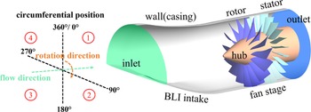
In this study, a BLI intake coupled with a single-stage subsonic fan was considered. The physical model is shown in Figure 1.
Display of physical model.

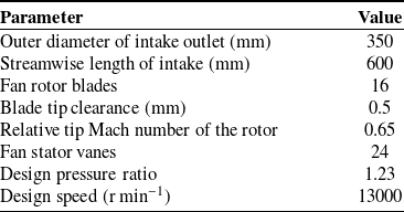
A small-offset, short-diffuser, splitterless layout with a D-shaped inlet and an exit outer diameter of 350 mm was adopted for the inlet. A rotor-stator blade-count ratio of 2:3, a design rotational speed of 13 000 r min−1 and a design stage pressure ratio of 1.23 were employed for the subsonic fan. The key design parameters of the integrated intake–fan configuration are summarised in Table 1.
2.3. Boundary conditions and solution settings
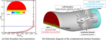
A BLI intake is an integral part of a propulsion system and it is installed on the mid-aft fuselage of a blended-wing-body aircraft. A full-fidelity simulation of the distorted inflow and the internal flow in the compression system requires coupling the intake, fuselage and external flow. This coupling is complex and time-consuming and is not well suited to theoretical analysis or detailed characterisation of the internal flow. Following related work (Rein, & Koch Reference Rein and Koch2015), in this research, a prescribed total-pressure boundary layer was imposed at the intake inlet whose thickness varied along the inlet height. Figure 2a shows the constructed distortion with a boundary-layer thickness of 0.20H, where H is the inlet height. The boundary conditions used in this study are shown in Figure 2b. Pressure-type boundaries were applied at both the inlet and the outlet. At the pressure-inlet boundary, the non-dimensional total-pressure profile in Figure 2a was imposed along with ambient pressure and temperature. At the pressure-outlet boundary, the static-pressure distribution was prescribed from the radial-equilibrium equation. All of the solid walls were set as adiabatic and no-slip. In the rotating domain, the fan rotational speed was prescribed.
In simulating a fan with inlet distortion, both the unsteady character of the distortion and the rotor–stator interactions had to be considered. Accordingly, a three-dimensional full-annulus URANS computation was performed for the domain used in this study. The k- $\omega$
shear-stress transport (SST) turbulence model was adopted to capture boundary-layer separation and shear-layer dynamics with adequate fidelity. For steady, incompressible flow, the transport equations of the turbulent kinetic energy k and the specific dissipation rate
$\omega$
shear-stress transport (SST) turbulence model was adopted to capture boundary-layer separation and shear-layer dynamics with adequate fidelity. For steady, incompressible flow, the transport equations of the turbulent kinetic energy k and the specific dissipation rate $\omega$
in the k-
$\omega$
in the k- $\omega$
SST model (Menter Reference Mårtensson and Billson1994) are given by
$\omega$
SST model (Menter Reference Mårtensson and Billson1994) are given by
 \begin{equation} \frac{\partial }{\partial t(\rho k)}+\frac{\partial (\rho kU_{i})}{\partial x_{i}}=\frac{\partial\!\left[(\mu +\sigma _{k}\mu _{t})\partial k/(\partial x_{j})\right]}{\partial x_{j}}+\tilde{G}_{k}-\rho \beta^{\ast}k\omega, \end{equation}
 \begin{equation} \frac{\partial }{\partial t(\rho \omega )}+\frac{\partial (\rho \omega U_{i})}{\partial x_{i}}=\frac{\partial\!\left[(\mu +\sigma _{\omega }\mu _{t})\partial \omega /(\partial x_{j})\right]}{\partial x_{j}}+\frac{\gamma }{\nu _{t}}\tilde{G}_{k}-\rho \beta \omega ^{2}+2\left(1-F_{1}\right)\rho \sigma _{\omega 2}\frac{1}{\omega }\frac{\partial k}{\partial x_{j}}\frac{\partial \omega }{\partial x_{j_{_{_{_{}}}}}}\!. \end{equation}
A steady RANS solution was first obtained to initialise the flow field, after which the computation was switched to URANS. The working fluid was modelled as an ideal gas. The component domains were connected via interface boundaries configured with no pitch scaling. The rotor-stator interface used a sliding-mesh (moving-mesh) approach to enable the real-time exchange of flow variables, ensuring consistent boundary conditions and continuous data transfer. Building on the URANS solution, a LES stage was then used to resolve details of the distorted flow. This strategy reduced the number of LES time steps required while maintaining accuracy, thereby significantly lowering the overall computational cost.
Key parameters of the intake and fan design

Boundary layer parameters and simulation boundary settings.

In a LES, the SGS turbulent stresses can be expressed as follows:
 \begin{equation} \tau _{ij}=\frac{1}{3}\tau _{kk}\delta _{ij}-2\mu _{t}\overline{S}_{ij}, \end{equation}
where $\mu _{t}$
and
$\mu _{t}$
and $\tau _{kk}$
are the sub-grid-scale turbulent viscosity and the isotropic part of the SGS stresses, respectively. The rate-of-strain tensor
$\tau _{kk}$
are the sub-grid-scale turbulent viscosity and the isotropic part of the SGS stresses, respectively. The rate-of-strain tensor $\overline{S}_{ij}$
can be expressed as
$\overline{S}_{ij}$
can be expressed as
 \begin{equation} \overline{S}_{ij}=\frac{1}{2}\left(\frac{\partial \overline{u}_{i}}{\partial x_{j}}+\frac{\partial \overline{u}_{j}}{\partial x_{i}}\right)\!. \end{equation}
In the LES for this study, the wall-adapting local eddy-viscosity (WALE) SGS model was employed to capture the unsteady flow dynamics (Dai et al. Reference Dai, Tang and Younis2022; Nicoud, & Ducros Reference Nicoud and Ducros1999). In the WALE model, the SGS eddy viscosity ( $\mu _{t}$
) is defined as
$\mu _{t}$
) is defined as
 \begin{equation} \mu _{t}=\rho {L}_{s}^{2}\frac{({S}_{ij}^{d}{S}_{ij}^{d})^{3/2}}{(\overline{S}_{ij}\overline{S}_{ij})^{5/2}+({S}_{ij}^{d}{S}_{ij}^{d})^{5/4}}. \end{equation}
In the expression, Ls
and ${S}_{ij}^{d}$
are defined as
${S}_{ij}^{d}$
are defined as
 \begin{equation} L_{s}=\textit{min}(kd,C_{w}V^{1/3}), \end{equation}
 \begin{equation} {S}_{ij}^{d}=\frac{1}{2}\left({\overline{g}_{ij}}^{2}+{\overline{g}_{ji}}^{2}\right)-\frac{1}{3}{\overline{g}_{kk}}^{2}\delta _{ij}, \end{equation}
 \begin{equation} \overline{g}_{ij}=\frac{\partial \overline{u}_{i}}{\partial x_{j}}. \end{equation}
The LES formulation was implemented in the commercial CFD solver Ansys Fluent.
Further numerical set-up details and verification are provided in § SI-A of the supplementary material available at https://doi.org/10.1017/flo.2026.10052, including the time-step and period settings, as well as the LES operating-point selection procedure. These additional materials further support the reliability and credibility of the numerical simulations presented in this work.
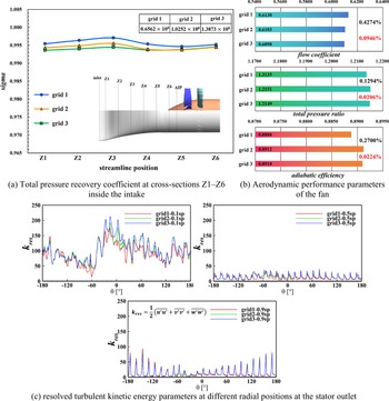
Grid independence.

2.4. Grid-independence verification and mesh characteristics
To assess the sensitivity of the numerical results to grid resolution, three meshes with different refinement levels were employed for the LES under identical operating conditions, denoted as grid 1, grid 2 and grid 3. The corresponding cell numbers were 65.62 million, 102.52 and 138.73 million, respectively.
Figure 3a compares the total pressure recovery coefficient at cross-sections Z1–Z6 along the intake. It can be seen that, with grid refinement, the distributions obtained on the three grids exhibit the same overall trend. The curves for grid 2 and grid 3 are almost indistinguishable, with only slight deviations in the S-shaped bend region (sections Z2 and Z3) where flow separation occurs. Although the coarse grid (grid 1) shows somewhat larger discrepancies, the overall differences remain modest, indicating that the internal flow in the fan intake is essentially grid-converged for the medium and fine grids. Furthermore, Figure 3b compares the global aerodynamic performance of the fan, including the flow coefficient, total pressure ratio and adiabatic efficiency. Taking the medium grid (grid 2) as the reference, the relative deviations of grid 1 in flow coefficient, total pressure ratio and adiabatic efficiency are approximately 0.4274 %, 0.1294 % and 0.2709 %, respectively, whereas those of the fine grid (grid 3) relative to grid 2 are only 0.0946 %, 0.0206 % and 0.0224 %. Therefore, the differences in the main aerodynamic parameters between the medium and fine grids are of the order of 0.1%, which is far below typical engineering tolerance. Beyond time-averaged mean quantities, the essence of evaluating LES fidelity lies in its capability to accurately capture turbulent fluctuations. To rigorously verify this, Figure 3c compares the circumferential distributions of the resolved turbulent kinetic energy (k res ) at three representative spanwise locations (10%, 50% and 90% span) at the stator outlet. As observed, while grid 1 locally underpredicts the peak turbulence intensities – particularly in the highly complex flow region near the hub at 0.1 span – the profiles for grid 2 and grid 3 collapse almost perfectly across all radial positions. This demonstrates that grid 2 has crossed the critical resolution threshold required to capture the energetic turbulent structures and unsteady dynamics.
Display of computational grid details.

In summary, grid 2 provides a satisfactory balance between accuracy and computational cost, and is thus adopted for all subsequent simulations.
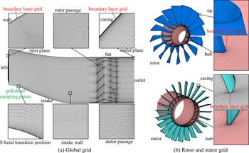
Having established the grid independence of the solution, the main characteristics of the computational mesh are summarised. Figure 4 presents the computational domain grids of the model. In this research, the domain consisted of three parts – the intake, the fan rotor and the stator – which were all discretised with structured hexahedral grids. The structured grids were generated primarily with Ansys ICEM and AutoGrid5. As shown in Figure 4a, the small S-shaped intake was gridded in ICEM using an O-type topology to improve the interior grid quality. A total of 445 grid points were uniformly distributed in the streamwise direction and boundary-layer grids were applied near the walls to achieve y + < 1. With this strategy, the intake contained approximately 21.67 million cells. The fan blades were refined using the automated AutoGrid5 module. For the rotor blade, a butterfly topology was adopted in the tip-clearance region to ensure grid quality and orthogonality. Figure 4b shows the grids of the fan and local details. Boundary-layer grids were also applied near the rotor and stator walls, with 15 layers. An O–4H topology was used around the blades, and the leading-edge (LE) and trailing-edge (TE) spacings were uniformly distributed. With this partitioning, the rotor domain consisted of approximately 32.28 million cells, the stator domain consisted of approximately 48.57 million cells and the total cell count of the full domain reached 102.52 million.
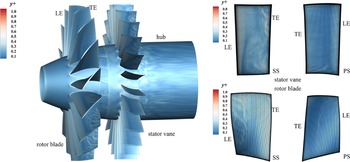
Refinement was applied to all of the near-wall grids of the fan that governed the internal aero-engine flow. As shown in Figure 5, y + stayed below 1.0 over the fan components and blade surfaces, except in the immediate LE and TE regions. On the stator, the maximum y + did not exceed 0.8. To meet LES resolution guidelines, the wall-unit spacings were set to Δx + ≤ 52.8248 and Δz + ≤ 56.4592 by locally increasing the grid density. Detailed validation and reliability assessment are provided in Appendix SI-A1.
Wall surface y + details.

3. Results and discussion
To examine the flow response and development mechanisms of inlet distortion with BLI, this study proceeded on two levels. First, because previous analyses largely relied on URANS, in this study, a side-by-side comparison of URANS and LES was performed under identical geometry and boundary conditions to establish a baseline, and assess where the two approaches agreed or diverged in capturing non-axisymmetric features, spatial distributions and key vortical structures. Second, to analyse the spatiotemporal evolution and uncertainty of the distorted flow, several representative time instants were selected. Within a time-resolved LES framework, in this study, the generation, interaction and decay of vortical structures inside the intake were analysed, the mechanism of the distortion propagating downstream from the inlet was delineated, and the potential impact of the distortion on the throughflow capacity and stability was evaluated. This two-tier analysis yielded a systematic understanding of BLI inlet distortion mechanisms.
3.1. Comparative study of flow field characteristics based on URANS and LES
3.1.1. Analysis of the distorted flow field in the intake
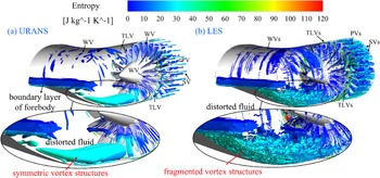
Figure 6 characterises the vortical structures across the integrated intake-fan domain using the Q-criterion. In the URANS results, the vortex system was comparatively simple. As the distorted low-energy fluid developed downstream, a symmetric vortex pair formed along the lower wall of the intake and remained circumferentially stable. Additional wall-bounded vortices (WVs) appeared on the intake, and on the rotor and stator surfaces due to boundary-layer effects. Within the fan stage, the topology was also straightforward, featuring the canonical rotor tip-leakage vortex (TLV), passage vortices (PVs) and shed vortices (SVs). In contrast, the LES revealed a more complete picture, resolving fine-scale vortex filaments and a fragmented vortex system throughout the domain rather than a few isolated coherent structures. The irregular downstream evolution of the distorted fluid manifested directly in the proliferation and breakdown of small-scale eddies. Within the fan, the rotor TLV was captured more sharply, which was advantageous for diagnosing loss mechanisms. Moreover, in the rotor–stator region, the adverse pressure gradient environment drove more vigorous mixing with the high-fidelity LES. Overall, the LES-based description was richer in spatial detail and better suited to analysing BLI-induced distortion and its associated losses.
Display of vortex structure inside the intake (dimensionless Q criterion = 0.01).

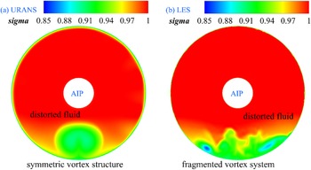
Total pressure distortion remained a central focus for this class of problems. Figure 7 compares the AIP total pressure distortion patterns to delineate the signatures and differences of the two approaches. As established earlier, the intake ingested a boundary layer of the same height. The downstream development of the low-energy fluid yielded distinct circumferential distortion patterns. In the URANS results, the contour was symmetric and circumferentially stationary, with a pair of symmetric vortex footprints as the dominant spatial feature. In contrast, the LES contour departed from this symmetry: the previously stable, symmetric pattern weakened, the circumferential extent of the distortion broadened and the compact vortex cores appeared as more dispersed patches on either side. Overall, the LES distortion pattern was less stationary than its URANS counterpart; yet, its azimuthal distribution and influence remained concentrated rather than uniform.
Comparison of AIP interface distortion pattern.

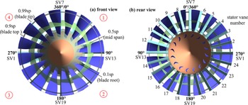
Schematic diagram of fan blade layout.

Details of fan rotor flow field with the distortion influence.

For a detailed description of the internal-flow analyses underlying the origin and downstream development of the AIP distortion – including meridional/axial flow features and three-dimensional streamlines – please refer to § SI-B.
3.1.2. Analysis of the internal flow field of the fan
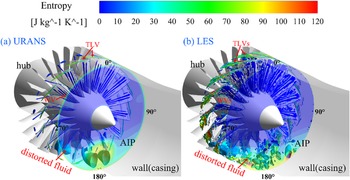
Figure 8 illustrates the circumferential indexing of the fan and the stator vane positions used in the analysis. In the figure, 0.99 sp denotes the spanwise station at the 99 % span (near the rotor blade tip). Figure 9 further contrasts the flow field structures within the rotor domain. As the distorted inflow convected downstream towards the fan, it continued to impinge on the rotor. A portion of the low-energy fluid passed through the rotor passages into the stator vane domain. Because of the direction of rotation, this distorted fluid was mainly concentrated in the rotor passages spanning 180°–270° in the azimuth. In the LES solution, the tip leakage vortices (TLVs) were captured more completely and, under the distorted inflow, the local leakage regions were associated with increased loss. These features differed from the simpler field predicted by URANS.
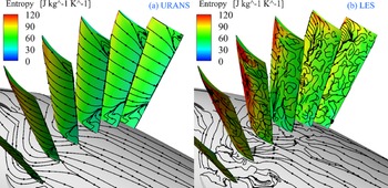
Figure 10 presents the rotor blade wall flow details and loss distributions within the distortion-affected sector. As shown in the surface limiting streamlines, the URANS solution appeared comparatively uniform. On both the rotor blade and the hub endwall, the patterns were steady, with no pronounced separation. In contrast, the LES solution revealed a different organisation at the same azimuth. A distinct separation followed by reattachment occurred near the LE on the suction side and the wall flow pattern was noticeably more disordered. The hub endwall pattern remained broadly similar to that of URANS. Entropy contours on the blade surface showed a clear entropy generation near the LE tip region for both methods. However, URANS predicted larger distortion-induced losses with more prominent entropy increase, whereas the LES yielded a lower peak magnitude but a broader affected area.
Flow topology of fan rotor blade surface in distortion-affected region.

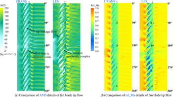
Figure 11 presents the S1 stream surface at the fan tip (0.99 sp) to compare the rotor response in the distortion-affected circumferential sector. The contours of the AVD and relative Mach number (Rel_Ma) showed pronounced differences in the tip leakage flow behaviour between the two approaches, which was consistent with the structures identified in Figure 9. In the LES solution, the tip leakage flow was highly unsteady and complex. The circumferential extent influenced by the distorted fluid was broader and its mixing with the tip leakage flow was stronger. In the URANS solution, the field was comparatively simple. The downstream transport of the distortion was more uniform and the affected region was smaller. These discrepancies carried into the stator vane domain, producing different patterns of aerodynamic penalty and loss.
Analysis of the fan tip flow field structure (0.99 sp).

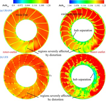
Figure 12 presents the S3 stream surface total pressure distributions at the rotor and the stator outlet. At the rotor outlet, the blade wakes were prominent at the same instant of time and both approaches were broadly consistent in this respect.
Analysis of the total distortion pattern of different S3 flow surfaces.

The difference was that the LES resolved the wall-bounded vortex systems on the rotor blades more finely. The downstream convection of the SVs was more evident and the transport of the tip leakage flow into the downstream field was visible in the contours. These features corroborated the preceding analysis. At the stator outlet, the discrepancies were larger. In the URANS solution, pronounced corner separation appeared in the stator domain, manifesting as both hub corner and casing corner separation, with the distorted fluid remaining concentrated in a limited circumferential sector. In the LES solution, the separation topology changed markedly. Corner separation persisted, but occurred mainly as hub corner separation dispersed across multiple stator passages and was present across the circumferential range, while casing separation was weakened. In addition, the shedding of the near-wall vortex systems produced fragmented vortices along the suction side in some passages. In the regions strongly affected by the distorted fluid, mixing between the distortion and the separated corner flow was evident, which inevitably increased stator losses. Notably, § SI-C provides additional analyses on the S1 flow surface parameters at multiple radial locations, which further elucidate the flow differences between the rotor and stator outlet planes discussed previously.
To further investigate the flow structure inside the stator passages, Figure 13 shows the vortical structures within the stator domain. It is evident from the figure that with the URANS method, the stator passages consisted of relatively simple vortical structures. The distorted fluid transmitted through the rotor was distributed in stator passages within the circumferential sector of 180°–270°, producing a blockage effect on the passage flow. A distinct vortex existed near the hub region on the suction surface of the stator vane. These vortices originated at the LE and shed near the TE along the streamwise direction. In addition, PVs were present within the stator passages and were fairly uniformly distributed around mid-span. The LES method showed a more complete vortex system. The stator passages are occupied by these vortical structures, and the passages dominated by the distorted fluid were likewise mainly concentrated in the 180°–270° sector, but with greater dispersion and stronger mixing with other PVs. Separation at the hub on the stator vane suction surface increased compared with the URANS field, and the flow uniformity within the stator passages deteriorated markedly.
Comparison of vortex structures in fan stator passages.

Figure 14 compares the stator vane wall flow details and loss distributions within the circumferential sector 180°–270°. Based on the surface limiting streamlines, the URANS solution appeared to be well behaved and fairly uniform. The patterns were steady and no aggravated separation was observed in this sector. Corner separation only occurred near the TE at the top and at the root. For the LES, the vane surfaces showed a different organisation. Distinct separation followed by reattachment arose near the suction side LE. The wall flow pattern was more disordered and the hub endwall region also exhibited new features that were consistent with the richer set of vortical structures captured by the LES.
Flow topology of fan stator vane surface in distortion-affected region.

The entropy contours further highlighted the differences. Both methods showed a pronounced entropy increase at the stator LE in this sector, but the magnitude was larger for the LES. The primary driver was the rotor and stator interaction. Unsteady rotor wakes impinged on the stator LE and increased the amount of loss. In the LES, the many vortical structures resolved within the passage mix into the flow and added to the loss, which was consistent with the limiting streamline patterns. Moreover, the distorted fluid packet captured by the LES spanned a wider circumferential extent and occupied more stator passages. This low-energy fluid contributed to additional loss and caused the entropy increase on the stator surface to be more prominent. These observations again demonstrate the advantage of LES in revealing the unsteady character of distortion-affected flows.
Figure 15 quantitatively compares the pitch-averaged flow angles at the stator inlet and outlet across different spanwise stations. The inlet flow angle ( $\alpha$
) and the outlet flow angle (
$\alpha$
) and the outlet flow angle ( $\beta$
) are defined as follows:
$\beta$
) are defined as follows:
 \begin{equation} \alpha =\frac{\arctan \left(\frac{Vt,\mathrm{in}}{V\alpha ,\mathrm{in}}\right)}{\pi }\times 180, \end{equation}
 \begin{equation} \beta =\frac{\arctan \left(\frac{Vt,\mathrm{out}}{V\alpha ,\mathrm{out}}\right)}{\pi }\times 180, \end{equation}
where $Vt$
and
$Vt$
and $V\alpha$
denote the local tangential and axial velocity components, respectively. The subscripts ‘in’ and ‘out’ denote the inlet and outlet measurement planes, respectively.
$V\alpha$
denote the local tangential and axial velocity components, respectively. The subscripts ‘in’ and ‘out’ denote the inlet and outlet measurement planes, respectively.
Comparison of inlet and outlet airflow angles in the stator domain.

For the circumferential distribution of $\alpha$
, the value increased from the root to the top. Near the root, the distortion had little influence. Consequently, both approaches yielded a largely uniform
$\alpha$
, the value increased from the root to the top. Near the root, the distortion had little influence. Consequently, both approaches yielded a largely uniform $\alpha$
around the circumference, with the LES predicting slightly lower values than URANS at the root. At the mid-span, the difference between the two methods was minimal, regardless of distortion. At the top, the distorted inflow sector introduced local increases and decreases in
$\alpha$
around the circumference, with the LES predicting slightly lower values than URANS at the root. At the mid-span, the difference between the two methods was minimal, regardless of distortion. At the top, the distorted inflow sector introduced local increases and decreases in $\alpha$
. Outside the distortion-affected sector, the two solutions showed no significant differences.
$\alpha$
. Outside the distortion-affected sector, the two solutions showed no significant differences.
In contrast, $\beta$
exhibited more pronounced differences with the LES because of the PVs and the presence of distorted fluid. The root region showed a marked loss of circumferential uniformity. By comparison, URANS produced smaller variations overall and maintained good circumferential uniformity. At the mid-span, the LES yielded slightly lower
$\beta$
exhibited more pronounced differences with the LES because of the PVs and the presence of distorted fluid. The root region showed a marked loss of circumferential uniformity. By comparison, URANS produced smaller variations overall and maintained good circumferential uniformity. At the mid-span, the LES yielded slightly lower $\beta$
than URANS over the azimuthal range, whereas at the top, it was slightly higher. Overall, in the URANS case, the circumferential distribution of
$\beta$
than URANS over the azimuthal range, whereas at the top, it was slightly higher. Overall, in the URANS case, the circumferential distribution of $\beta$
remained relatively uniform.
$\beta$
remained relatively uniform.
Figure 16 compares the pitch-averaged Mach numbers (Ma) at the stator inlet and outlet across different spanwise stations to assess the change in the aerodynamic parameters through the stator. Upstream of the stator, the inlet Ma varied with the radius as the flow field changed. Both approaches showed a decreasing trend in the stator inlet Ma from root to top, which was closely linked to the variation of $\alpha$
. Due to the influence of the rotor tip-leakage transport and the distorted inflow, the throughflow capacity near the stator LE at the top was reduced. Overall, the circumferential distributions from the two methods remained fairly uniform at the stator inlet and the numerical differences were small.
$\alpha$
. Due to the influence of the rotor tip-leakage transport and the distorted inflow, the throughflow capacity near the stator LE at the top was reduced. Overall, the circumferential distributions from the two methods remained fairly uniform at the stator inlet and the numerical differences were small.
Comparison of inlet and outlet pressure coefficients in the stator domain.

At the stator outlet, the throughflow differed markedly, especially near the root. This confirmed the adverse impact of the root corner separation. In the LES results, the aerodynamic performance downstream of the stator root deteriorated significantly and the flow non-uniformity was notably stronger. In the URANS case, the root corner separation inside the stator passages was less pronounced, so both the throughflow capacity and the circumferential uniformity were better than those in the LES. For the mid-span and top regions, the two methods predicted similar trends, with only minor quantitative differences.
Considering the Ma upstream and downstream of the stator, the root separation induced the largest throughflow decay after the stator’s straightening action. Taken together with the preceding analysis, the LES was more effective in revealing the throughflow reduction and its causes at the stator root.
3.2. Time-resolved analysis of unsteady flow evolution based on the LES
A comprehensive comparison between URANS and LES showed that LES more fully revealed the effects of the BLI inlet distortion, the spatiotemporal distribution of the distortion pattern, and key flow parameters in the rotor and stator passages. It also described the unsteady behaviour of the integrated intake–fan system more effectively. Based on this, in this research, three representative LES time instants were analysed: t1 , t2 and t3 . Here, t1 denotes the initial transient phase, t2 is the calculation time of the transition phase and t3 is the time of the statistically stationary phase. In this research, the generation and transport of the distorted inflow within the passages, its coupling with the rotor and stator flow fields, and the evolution of those fields were evaluated. The results provide numerical evidence for the unsteady mechanisms and the fan response with BLI distortion.
3.2.1. Development characteristics of unsteady distorted fluids
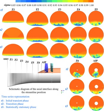
Based on the total pressure recovery coefficient contour shown in Figure 17, the distorted fluid exhibited pronounced circumferential non-uniformity from the inlet onward. From Z1 to Z2, the low-energy fluid persisted as a wall-attached thin layer and a shear layer with sharp boundaries. At Z3, the low-energy region thickened and rolled-up vortical textures appeared, indicating that shear-layer instability began to dominate. At Z4–Z5, the low-energy region spread laterally and became patchy, and the local minimum occurred on the lower side at an intermediate radius, showing that the secondary flow lifted and entrained the low-energy fluid. By Z6 and at the AIP, the low-energy packet broke into finer multiscale structures yet remained confined to a fixed circumferential sector, indicating strong trackability and phase stability for the distortion core.
Distortion pattern of the flow interface inside the intake for different time series.

Ultimately, it reached the fan as a non-axisymmetric inflow. Based on the LES time evolution, the flow was the most unsteady at t1 and the distorted fluid structures were not yet fully developed. At t2 , the distorted fluid began to transition towards a stable stage. The boundary textures of the low-energy fluid were the richest, indicating peak secondary-flow activity and shear-layer instability. At t3 , the distortion contour became smoother and its amplitude rose slightly. The time-averaged distortion produced by thorough mixing became dominant, while the circumferential phase was largely preserved. This indicated that a stable and pronounced distorted sector remained at the AIP, which was likely to induce circumferentially non-uniform inlet loading, reduce the stability margin and amplify the rotor–stator interaction noise.
Figure 18 compares the three-dimensional unsteady features of the intake vortical structures at the three instants. A time sequence of the lower wall vortex patterns and the meridional plane axial vorticity showed the following. At t1 , the boundary-layer fluid was ingested, and for the adverse pressure gradient and curvature along the lower wall, a wall-attached shear layer was formed. It appeared as alternating positive–negative axial vorticity streaks and a fragmented vortex system, and the low-energy fluid was mainly convected along the wall. At t2 , the low-energy fluid and the vortical structures began to transition towards a more stable state, and the distortion changed from band-like to multiscale patchy patterns. This was consistent with the texture-rich pattern and the downward shift of the low-energy fluid at Z3–Z5 shown in Figure 17. At t3 , large-scale structures in the intake broke down further. The amplitude decreased slightly, but the circumferential phase of the distortion became more stable and the low-energy vortical packets continued to convect downstream to the AIP. These features revealed the development of the distortion vortex core with BLI.
Internal vortex structure and temporal evolution characteristics of intake.

3.2.2. Characteristics of the fan’s rotor flow field
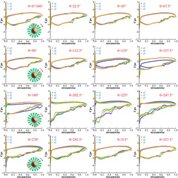
At different instants, the distorted flow field showed different features and the impact on the downstream fan changed accordingly. This time-dependent behaviour is discussed in § SI-D1. Figure 19 further shows the surface pressure coefficient (Cps) distributions at the 90 % span of the rotor blade, evaluated at various circumferential angles (θ) for the three time instants. The Cps is defined as
 \begin{equation} \mathrm{Cps}=\frac{p_{s}-p_{s,\mathrm{in}}}{{p}_{t,\mathrm{in}}^{*}-p_{s,\mathrm{in}}}, \end{equation}
where $p_{s}$
is the static pressure on the blade surface, and
$p_{s}$
is the static pressure on the blade surface, and $p_{s,\mathrm{in}}$
and
$p_{s,\mathrm{in}}$
and ${p}_{t,\mathrm{in}}^{*}$
represent the averaged static pressure and the averaged total pressure at the inlet, respectively.
${p}_{t,\mathrm{in}}^{*}$
represent the averaged static pressure and the averaged total pressure at the inlet, respectively.
Pressure coefficient distribution of the 90 % span on rotor blades at various circumferential angles for different time series.

Based on the variation of these pressure coefficients, the discussion proceeds as follows.
First, considering the overall distribution of the Cps, at most circumferential positions, the Cps distribution exhibited the typical aerodynamic pattern of a rotor blade: a pronounced suction peak appeared at the LE, the Cps dropped sharply and then gradually recovered along the chord, and the curves tended to merge near the TE. This meant that, overall, the blade at the 0.9 span still maintained a lift-type aerodynamic loading distribution.
Second, in terms of circumferential differences, within θ = 0°–90°, the suction-side peak was concentrated and the differences among the three instants were small, which indicated relatively uniform inflow and stable aerodynamic loading in this circumferential range. Within θ = 135°–247.5°, the Cps curves showed clear bifurcation and time-sequence differences, especially at θ = 180° and θ = 225°. The LE suction peak fluctuated strongly, with large peak differences from t1 to t3 . This indicated that this sector was the most strongly affected by inlet distortion, with unsteady phenomena such as local increases in incidence, boundary-layer separation and reattachment. However, within θ = 270°–360°, the Cps distribution gradually returned to a regular pattern and the three curves nearly coincided, indicating that the inflow in this sector became uniform again and the unsteadiness weakened.
Finally, in terms of temporal characteristics, in the sector strongly affected by distortion (θ = 180°–225°), the differences among t1 , t2 and t3 were significant, which indicated strong temporal instability of the local flow field and the passage of unsteady vortical structures over the blade surface. In the sectors that were weakly affected by distortion (θ = 270°–360°), the three curves agreed well, indicating that the flow was essentially steady. This circumferential progression – from stable to unstable and back to stable – corresponded to the spatial distribution of the distorted inflow at the fan inlet section and its modulation over time.
Based on the above flow field analysis, the distorted fluid produced pronounced non-uniformity in the rotor passages at different instants. This circumferential pattern revealed the direct influence of the asymmetry on the rotor blade loading, with especially large differences among the three instants at θ = 180° and θ = 225°. The LE suction peak was elevated at these angles, indicating that the distorted inflow triggered a strong unsteady aerodynamic response, which in turn increased local aerodynamic losses and surface dissipation. The transiently deep negative pressure peak also implied that the critical incidence was more readily reached, potentially triggering local separation and thereby reducing the fan’s stability margin and overall performance.
3.2.3. Characteristics of the fan’s stator flow field
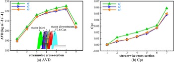
For the flow inside the stator, Figure 20 combines the AVD and the total-pressure loss coefficient (Cpt) to further quantify the throughflow capacity and the flow losses at different streamwise cross-sections. The Cpt is defined as
 \begin{equation} \mathrm{Cpt}=\frac{{p}_{t,\mathrm{in}}^{*}-{p}_{t}^{*}}{{p}_{t,\mathrm{in}}^{*}-p_{s,\mathrm{in}}}, \end{equation}
where ${p}_{t}^{*}$
is the averaged total pressure at the streamwise cross-section.
${p}_{t}^{*}$
is the averaged total pressure at the streamwise cross-section.
Characteristics of the AVD and Cpt changes in different streamwise cross-sections within the stator.

Figure 20a shows that the AVD increased monotonically from stator inlet section 1 along the streamwise direction, reached a peak at section 6 and then decreased at section 7 downstream of the stator TE. This indicates that the throughflow capacity was the strongest in the mid-to-aft part of the stator, while the downstream section weakened overall. For the Cpt, the value increased monotonically throughout the stator domain. At the downstream region of section 7, the linear growth rate was larger and the amount of the loss rose markedly. In terms of time evolution, both of the parameters followed the same trend at the three instants. Because the upstream flow was highly unsteady at t1 , the differences were more pronounced than those at t2 and t3 . Between the transitional instant t2 and the stable instant t3 , the parameter differences were minor.
Figure 21 uses AVD contours to further explain the changes in the flow parameters inside the stator. The figure shows a comparison of the upstream and downstream sections (sections 1 and 7) at the three time instants in detail. In section 1, the flow distribution was almost the same at all three instants. Continuous convection of the upstream distorted fluid and the leakage flow reduced the circumferential uniformity at the inlet, and the distorted fluid accumulated in a concentrated sector. As the solution converged, the forms of the distorted and leakage flows showed slight differences. After the flow passed through the stator passages, section 7 showed extensive root corner separation that occupied multiple stator passages around the circumference. The accumulation of low-energy fluid reduced the overall throughflow capacity and increased the flow loss. This was consistent with the trends shown in Figure 20. At different instants, the distorted fluid downstream of the stator mixed with the root corner separation. As the flow approached a stable state, this unsteady component disappeared, whereas the circumferentially distributed root corner separation remained. Further details on the corner separation, together with the low-energy-fluid regions, are provided in § SI-D2.
Comparison of AVD contours at positions 1 and 7 of the cross-section for different time series.

Figure 22 compares the stator vane surface loss states across four circumferential sectors. The figure reveals the circumferential and temporal characteristics of the entropy production inside the stator passages. In the overall circumferential distribution, the entropy field was strongly non-uniform. In sector 3, where the distorted inflow had the greatest influence, high-entropy features were evident and azimuthally extensive, and at the three time instants, the distortion-induced loss appeared differently on the vane surfaces. At t1 , for non-uniform upstream inflow, the eighth stator vane in sector 1 showed a clear entropy increase, while the other vane surfaces showed no obvious increase. In sector 2, the LE entropy increase was evident and on some vanes, a high-entropy band extended from the hub to the tip near the LE. In sector 3, multiple vane surfaces exhibited high-entropy patches, whereas in sector 4, there was no significant entropy increase. As the solution advanced to t2 , the vane surface entropy distribution changed in sectors 1–3, while sector 4 showed no marked change. The most prominent change was that the originally large high-entropy region in sector 2 shrank significantly, whereas the high-entropy region in sector 3 increased markedly. This pattern was essentially maintained at t3 .
Characteristics of the entropy distribution of the stator vanes in different sectors for different time series.

Building on the preceding flow analysis, the changes in entropy generation were driven by the development and stabilisation of the distorted fluid. During its transport at t1 , the distorted fluid expanded circumferentially, so larger losses appeared in sectors 2 and 3. As the flow became stable, the distortion was concentrated in sector 3 and the associated loss increased markedly. Beyond the distortion itself, upstream-flow interference could still raise the vane surface loss locally in the circumferential direction, as seen in the increased LE loss on some vanes in sector 1. A qualitative comparison across sectors showed that the loss distribution inside the stator passages was sector-fixed and circumferentially continuous. This pattern was the root cause of the non-uniform flow at the stator outlet and the key issue to address when improving the outlet flow uniformity.
4. Conclusions
Based on the numerical simulations in this research, the following conclusions were reached.
-
(i) Relative to URANS, LES provided a more complete and finer description of the BLI inlet distortion, including the spatiotemporal distribution of the distortion pattern, and the key parameters within the rotor and stator passages. It characterised the unsteady behaviour of the integrated intake–fan system more effectively. The LES-resolved flow field exhibited a more complex three-dimensional organisation, and the distorted fluid was more unsteady in both the circumferential and radial directions.
-
(ii) LES resolved the fragmented vortex system inside the fan, with clear advantages in capturing the formation, evolution and mixing of TLVs. The distorted fluid covered a broader circumferential extent and mixed more strongly with the tip-leakage flow, which strengthened the local unsteady response and increased the amount of loss. LES also identified root throughflow limitation and corner separation in the stator with more sensitivity, indicating a stronger reduction of the hub throughflow capacity and offering greater potential for diagnosing internal loss.
-
(iii) The time-sequenced LES results showed that the intake vortical structures were strongly three-dimensional and unsteady. The distortion core evolved in time; yet, the circumferential phase of the distortion pattern remained largely preserved. A stable sector with pronounced distortion therefore persisted on the AIP, producing sustained circumferential nonuniformity of the inlet loading.
-
(iv) Across the three instants, the influence of the distorted fluid on the fan remained concentrated in sector 3. For the rotor, the distorted inflow in this sector more readily approached critical incidence and triggered local separation, which increased surface dissipation and aerodynamic loss. For the stator, the hub side suction surface corner separation was more prominent, and the loss distribution within the stator passages was sector-fixed and circumferentially continuous, which degraded the overall performance and the stability margin.
The precise identification of the sector-fixed loss pattern and severe flow deterioration provides crucial azimuthal guidance. Consequently, this work establishes a rigorous physical validation for employing localised, sector-specific stator modifications, thereby paving the way for targeted distortion-tolerant design optimizations in future boundary layer ingestion propulsion systems.
Supplementary material
The supplementary material for this article can be found at https://doi.org/10.1017/flo.2026.10052.
Acknowledgments
We thank the Zhejiang Key Laboratory of Industrial Intelligence and Digital Twin, Eastern Institute of Technology, Ningbo, for providing ample computational resources.
Data availability statement
The data that support the findings of this study are available from the corresponding author upon reasonable request.
Funding statement
This work was supported in part by the National Natural Science Foundation of China (Grant No. 12302346).
Competing interests
The authors declare that there is no conflict of interest regarding the publication of this article.
Statement on the use of AI
The authors also used the AI language model ChatGPT to assist with English language editing and improving the clarity of the manuscript; all numerical simulations, physical interpretations and conclusions are solely the work of the authors.







 Open access

