





Impact Statement
Quantifying how canopy geometry controls aerodynamic drag is a central challenge in environmental flows and wind engineering. Traditional descriptors based on single parameters, such as packing density or frontal area, provide only coarse characterisations and fail to capture the spatial heterogeneity governing canopy–flow interactions. This work introduces a data-driven approach that learns low-dimensional, physically interpretable latent representations of canopy configurations directly from geometry using a convolutional variational autoencoder with disentanglement regularisation. The learned latent variables correspond to fundamental geometric features influencing drag, including effective canopy occupancy and streamwise packing asymmetry, and are quantitatively linked to experimentally measured drag coefficients without resolving flow fields. By providing a compact and interpretable mapping between complex canopy geometry and aerodynamic response, this approach enables efficient drag prediction, supports reduced-order modelling, and facilitates systematic exploration of canopy and roughness designs relevant to natural and engineered environments.
1. Introduction
The interaction between vegetative canopies and turbulent flows plays a central role in regulating momentum exchange, mixing processes, and drag in both natural and engineered environments. Canopies introduce strong shear layers, energetic coherent structures and wake interactions that fundamentally modify turbulence relative to smooth-wall boundary layers. These effects govern drag force and, in turn, influence ecosystem–atmosphere exchanges, fluvial and coastal morphodynamics, urban microclimates, and bio-inspired flow-control strategies. Despite extensive studies, the multiscale coupling between canopy geometry, turbulence and drag remains incompletely understood, and continues to motivate integrated approaches that combine detailed measurements, physical modelling and data-driven analysis.
In general, canopy flows can be classified into three representative regimes based on the spacing between canopy elements or patches: isolated roughness flow, wake interference flow and skimming flow (Folkard Reference Folkard2011; Mayaud et al. Reference Mayaud, Wiggs and Bailey2016). In sparse canopies, wakes shed by individual elements evolve independently and total drag approximates the sum of element-scale contributions. As packing density increases, wake interference alters the mean flow and turbulence. In a sufficiently dense scenario, a canopy behaves as a quasi-continuous roughness layer in which flow largely skims over the top, with limited penetration into the interior. These regimes are commonly parameterised using the packing density, $\lambda _p$
, defined as the ratio of canopy-occupied area to the total floor area. Numerous studies have explored how variations in
$\lambda _p$
, defined as the ratio of canopy-occupied area to the total floor area. Numerous studies have explored how variations in $\lambda _p$
affect gap-scale turbulence (Chung et al. Reference Chung, Mandel, Zarama and Koseff2021; Folkard Reference Folkard2011, Reference Folkard2005), coherent structures at canopy interfaces (Maltese et al. Reference Maltese, Cox, Folkard, Ciraolo, La Loggia and Lombardo2007) and canopy-induced hydraulic resistance (Savio et al. Reference Savio, Vettori, Biggs, Zampiron, Cameron, Stewart, Soulsby and Nikora2023). Recent efforts have extended these analyses to fully three-dimensional (3-D) canopy flows, revealing complex wake interactions and turbulent structures (Li and Giometto Reference Li and Giometto2024; Lopez de la Cruz et al. Reference Lopez de la Cruz, Haward and Shen2025; Park and Nepf Reference Park and Nepf2025; Rota et al. Reference Rota, Monti, Olivieri and Rosti2024; Sathe and Giometto Reference Sathe and Giometto2024; Song et al. Reference Song, Wang, Duan, Stocchino and Yan2024).
$\lambda _p$
affect gap-scale turbulence (Chung et al. Reference Chung, Mandel, Zarama and Koseff2021; Folkard Reference Folkard2011, Reference Folkard2005), coherent structures at canopy interfaces (Maltese et al. Reference Maltese, Cox, Folkard, Ciraolo, La Loggia and Lombardo2007) and canopy-induced hydraulic resistance (Savio et al. Reference Savio, Vettori, Biggs, Zampiron, Cameron, Stewart, Soulsby and Nikora2023). Recent efforts have extended these analyses to fully three-dimensional (3-D) canopy flows, revealing complex wake interactions and turbulent structures (Li and Giometto Reference Li and Giometto2024; Lopez de la Cruz et al. Reference Lopez de la Cruz, Haward and Shen2025; Park and Nepf Reference Park and Nepf2025; Rota et al. Reference Rota, Monti, Olivieri and Rosti2024; Sathe and Giometto Reference Sathe and Giometto2024; Song et al. Reference Song, Wang, Duan, Stocchino and Yan2024).
While 3-D flow analyses have improved our understanding of canopy–turbulence interactions, canopy geometries in most studies remain highly idealised. Typical configurations rely on uniform, staggered or random arrays of elements (Buccolieri et al. Reference Buccolieri, Wigö, Sandberg and Di Sabatino2017; Liu et al. Reference Liu, Huai and Ji2021; Nicolle and Eames Reference Nicolle and Eames2011; Taddei et al. Reference Taddei, Manes and Ganapathisubramani2016). Yet local geometric perturbations are known to produce substantial variations in drag (Maza et al. Reference Maza, Lara and Losada2015), and even the placement of a single element can alter wake development and element-scale loadings (Tinoco et al. Reference Tinoco, San Juan and Mullarney2020). This sensitivity highlights a broader challenge: the relationship between canopy topography and resulting drag is high-dimensional, nonlinear and not easily described using coarse statistics such as packing density alone.
A robust description of canopy topography is thus central to advancing our understanding of canopy–flow interactions. Traditional descriptors such as packing density or frontal area index provide interpretable global measures, but fail to capture the complex spatial organisation of canopy elements. Emerging tools from deep learning, including autoencoders (Kingma and Welling Reference Kingma and Welling2013; Ng et al. Reference Ng2011; Van Den Oord et al. Reference Van Den Oord, Vinyals and Kavukcuoglu2017; Burgess et al. Reference Burgess, Higgins, Pal, Matthey, Watters, Desjardins and Lerchner2018; Chen et al. Reference Chen, Li, Grosse and Duvenaud2018; Fukami and Taira Reference Fukami and Taira2023; Fukami et al. Reference Fukami, Iwatani, Maejima, Asada and Kawai2025; Meo et al. Reference Meo, Mahon, Goyal and Dauwels2024) and compressed sensing (Bristow et al. Reference Bristow, Eriksson and Lucey2013; Sreter and Giryes Reference Sreter and Giryes2018; Xiao et al. Reference Xiao, Qiu, Ha, Bani, Zhou and Sotiras2025), offer new opportunities to learn compact, data-driven representations of canopy geometry. By projecting high-dimensional data snapshots onto lower-dimensional latent manifolds, these approaches preserve detailed structural information while enabling interpretability, generative modelling and integration with downstream physical inference tasks. For example, Fukami and Taira (Reference Fukami, Iwatani, Maejima, Asada and Kawai2025) proposed an observable-augmented manifold learning approach that compresses and distinguishes multi-source turbulent flow data into a unified low-dimensional latent representation by incorporating the Reynolds number dependence of data snapshots. A similar approach was also developed by Tran et al. (Reference Tran, Fukami, Inada, Umehara, Ono, Ogawa and Taira2024) using the drag coefficient to assist the identification and regularisation of low-dimensional geometric latent space for industrial vehicle geometry design and optimisation. Although the latter study employed a methodology similar to our framework, the present approach further advances observable-augmented modelling by emphasising the interpretability of the learned representation through disentanglement techniques in representation learning (Burgess et al. Reference Burgess, Higgins, Pal, Matthey, Watters, Desjardins and Lerchner2018; Chen et al. Reference Chen, Li, Grosse and Duvenaud2018; Meo et al. Reference Meo, Mahon, Goyal and Dauwels2024).
Here, we present a comprehensive analysis of the mapping between canopy topography and its associated drag characteristics. We propose a convolutional variational autoencoder (VAE) architecture based on PixelCNN (Kolesnikov and Lampert Reference Kolesnikov and Lampert2017; Van den Oord et al. Reference Van den Oord, Kalchbrenner, Espeholt, Vinyals and Graves2016) that learns disentangled latent generative factors of canopy configurations tied to the observed drag coefficient, enabling a geometric interpretation and accurate drag prediction. Our analysis is supported by an extensive wind tunnel dataset comprising over 2000 experiments with three flow speeds, spanning three representative packing densities and five filling ratios, with approximately 900 distinct canopy configurations. The paper is structured as follows: in § 2, we describe the experimental setup, geometric features of the artificial canopy models, and parameters of the datasets. In § 3, we discuss the representations of canopy configurations and the proposed VAE model. In § 4, we present the low-dimensional latent space with auxiliary observables. Discussion is elaborated in § 5 and main conclusions are given in § 6.
2. Experimental set-up
Laboratory experiments were conducted in the Talbot wind tunnel at the University of Illinois Urbana–Champaign. The Eiffel-type facility has a test section 6 m long, 0.914 m wide and 0.46 m high, and its flow characteristics are documented by Adrian et al. (Reference Adrian, Meinhart and Tomkins2000). All experiments were performed near the inlet of the test section, where the incoming boundary layer is negligible, ensuring a nominally uniform approach flow.
The study considered 2046 distinct rectangular canopy patch configurations composed of identical vertical elements arranged on a square lattice. The configurations were organised into three geometric types, defined by the spacing and number of potential element locations. In the first type, canopy elements with square base area $a \times a$
(
$a \times a$
( $a=10$
mm) could be placed on a
$a=10$
mm) could be placed on a $5 \times 5$
grid with streamwise and transverse spacings of
$5 \times 5$
grid with streamwise and transverse spacings of $5a$
. The second type consisted of a
$5a$
. The second type consisted of a $10 \times 10$
grid with spacings of
$10 \times 10$
grid with spacings of $3a$
, while the third type comprised a
$3a$
, while the third type comprised a $15 \times 15$
grid with spacings of
$15 \times 15$
grid with spacings of $2a$
. These three arrangements correspond to packing densities
$2a$
. These three arrangements correspond to packing densities $\lambda _p=0.04$
, 0.11 and 0.25, respectively, and define the local geometric spacing between neighbouring elements. For each packing density, combinations of randomly generated and customised configurations were examined.
$\lambda _p=0.04$
, 0.11 and 0.25, respectively, and define the local geometric spacing between neighbouring elements. For each packing density, combinations of randomly generated and customised configurations were examined.
For each geometric type, the number of elements present on the base plate was varied through a filling ratio $\eta$
, defined as the fraction of available element locations that were occupied. For all three packing densities, filling ratios of 40 %, 60 % and 80 % were tested. For the two denser layouts (
$\eta$
, defined as the fraction of available element locations that were occupied. For all three packing densities, filling ratios of 40 %, 60 % and 80 % were tested. For the two denser layouts ( $\lambda _p=0.11$
and 0.25), additional sparse cases with
$\lambda _p=0.11$
and 0.25), additional sparse cases with $\eta =10\,\,\%$
and 20 % were also considered as a complement. A large fraction of the configurations were generated randomly using a two-dimensional binomial distribution
$\eta =10\,\,\%$
and 20 % were also considered as a complement. A large fraction of the configurations were generated randomly using a two-dimensional binomial distribution $\sim B(N_c,0.5)$
, where
$\sim B(N_c,0.5)$
, where $N_c$
is the number of elements present. To ensure a constant maximum spanned frontal width for a given packing density, configurations containing empty spanwise columns were discarded and replaced with realisations that fully occupied the outermost columns. In addition to the random realisations, a limited number of customised configurations were designed to probe specific geometric motifs. The distribution of configurations across packing densities and filling ratios is summarised in Table 1. While the packing density
$N_c$
is the number of elements present. To ensure a constant maximum spanned frontal width for a given packing density, configurations containing empty spanwise columns were discarded and replaced with realisations that fully occupied the outermost columns. In addition to the random realisations, a limited number of customised configurations were designed to probe specific geometric motifs. The distribution of configurations across packing densities and filling ratios is summarised in Table 1. While the packing density $\lambda _p$
characterises the local spacing between neighbouring elements and the filling ratio
$\lambda _p$
characterises the local spacing between neighbouring elements and the filling ratio $\eta$
controls the fraction of occupied sites, neither parameter alone fully describes the overall canopy denseness. We therefore define the effective canopy occupancy
$\eta$
controls the fraction of occupied sites, neither parameter alone fully describes the overall canopy denseness. We therefore define the effective canopy occupancy $\xi =\lambda _p\eta$
, which represents the ratio of total canopy frontal area to the total floor area of interest. A fully dense, solid-body canopy corresponds to
$\xi =\lambda _p\eta$
, which represents the ratio of total canopy frontal area to the total floor area of interest. A fully dense, solid-body canopy corresponds to $\xi =1$
, whereas an empty base plate yields
$\xi =1$
, whereas an empty base plate yields $\xi =0$
.
$\xi =0$
.
Summary of canopy configurations tested across packing densities $\lambda _p$
, filling ratios
$\lambda _p$
, filling ratios $\eta$
and free stream velocity levels
$\eta$
and free stream velocity levels $U_\infty$
. Asterisks denote customised (non-random) configurations
$U_\infty$
. Asterisks denote customised (non-random) configurations

Each canopy configuration was made using a modular base plate and identical vertical elements fabricated from ABS using a Bambu Lab H2D 3-D printer. The base plate measured $300 \times 300 \times 10.5$
mm and contained a regular Cartesian array of square insertion holes, each 10 mm
$300 \times 300 \times 10.5$
mm and contained a regular Cartesian array of square insertion holes, each 10 mm $\times$
10 mm base area, corresponding to the three lattice types described above. The canopy elements were rectangular rods of dimensions
$\times$
10 mm base area, corresponding to the three lattice types described above. The canopy elements were rectangular rods of dimensions $10 \times 10 \times 107$
mm and were inserted additional 7 mm into the base plate, resulting in an exposed height of
$10 \times 10 \times 107$
mm and were inserted additional 7 mm into the base plate, resulting in an exposed height of $H=100$
mm. The exposed frontal area of a single element normal to the flow was therefore
$H=100$
mm. The exposed frontal area of a single element normal to the flow was therefore $A_c=100$
mm
$A_c=100$
mm $\times$
10 mm = 1000 mm
$\times$
10 mm = 1000 mm $^2$
.
$^2$
.
The drag coefficient $C_D$
was defined using the maximum spanned frontal area of the canopy configuration,
$C_D$
was defined using the maximum spanned frontal area of the canopy configuration, $A=H\times W$
,
$A=H\times W$
, $C_D=F_D/[\frac {1}{2}\rho U_\infty ^2 A]$
, where
$C_D=F_D/[\frac {1}{2}\rho U_\infty ^2 A]$
, where $F_D$
is the mean drag force,
$F_D$
is the mean drag force, $\rho =1.23$
kg m
$\rho =1.23$
kg m $^{-3}$
is the air density,
$^{-3}$
is the air density, $H=0.1$
m is the element height and
$H=0.1$
m is the element height and $W$
is the maximum transverse extent of the canopy. Because
$W$
is the maximum transverse extent of the canopy. Because $W$
depends on the lattice type, its value varied slightly with packing density:
$W$
depends on the lattice type, its value varied slightly with packing density: $W=0.21$
m for
$W=0.21$
m for $\lambda _p=0.04$
,
$\lambda _p=0.04$
, $0.28$
m for
$0.28$
m for $\lambda _p=0.11$
and
$\lambda _p=0.11$
and $0.29$
m for
$0.29$
m for $\lambda _p=0.25$
, corresponding to frontal areas of
$\lambda _p=0.25$
, corresponding to frontal areas of $A=0.021$
, 0.028 and 0.029 m
$A=0.021$
, 0.028 and 0.029 m $^2$
, respectively.
$^2$
, respectively.
Drag measurements were performed by mounting each canopy patch normal to the incoming flow and instrumenting it with an ATI Gamma six-axis force/torque sensor positioned beneath the base plate. The sensor measured the instantaneous drag acting on the entire canopy configuration. Force signals were sampled at 1 kHz over 30 s for each run. Measurements were conducted at up to three free stream velocities, $U_\infty =11.5$
, 16.3 and 21.1 m s
$U_\infty =11.5$
, 16.3 and 21.1 m s $^{-1}$
, depending on the configuration, to assess drag consistency. Because drag is invariant under mirror symmetries of the canopy layout, geometrically reflected configurations were treated as dynamically equivalent, yielding a total of 4092 valid distinct drag measurements across all velocities.
$^{-1}$
, depending on the configuration, to assess drag consistency. Because drag is invariant under mirror symmetries of the canopy layout, geometrically reflected configurations were treated as dynamically equivalent, yielding a total of 4092 valid distinct drag measurements across all velocities.
To ensure accurate drag measurements and prevent flow leakage beneath the canopy base plate, a perimeter assembly was designed to divert the incoming flow above and around the plate. The assembly consisted of front, rear, left and right sections fabricated by 3-D printing. The front and rear sections featured quarter-ellipsoidal cross-sections with semi-minor-to-major axis ratios of 1:3, followed by rectangular extensions, providing a smooth transition for the incoming flow. During experiments, the perimeter assembly was positioned approximately 2 mm away from the base plate to avoid mechanical contact while minimising leakage. Narrow slots along the bottom of each section housed neodymium magnets, which were paired with matching magnets placed on the opposite side of the thin aluminium ceiling of the wind-tunnel test section, providing secure magnetic attachment without introducing additional loads on the force sensor. A schematic of the assembled canopy, perimeter assembly and lattice layouts is shown in Figure 1.
Schematic of the experimental set-up. (a) Canopy patch mounted on a load cell with a perimeter assembly to guide the incoming flow $U_\infty$
. (b) Base-plate arrays defining the packing density
$U_\infty$
. (b) Base-plate arrays defining the packing density $\lambda _p$
:
$\lambda _p$
: $5\times 5$
(0.04),
$5\times 5$
(0.04), $10\times 10$
(0.11) and
$10\times 10$
(0.11) and $15\times 15$
(0.25).
$15\times 15$
(0.25).

3. Data-driven modelling
3.1. Canopy configuration representation
Canopy configurations were represented using a discrete, top-down encoding inspired by digital elevation models. Viewed from above, each potential element location was assigned a value of 1 if occupied by a canopy element and 0 otherwise, yielding a binary lattice representation. Each configuration was thus encoded as a $30\times 30$
binary matrix, referred to as a Bernoulli canopy map, with rows ordered in the streamwise direction such that the first row encounters the incoming flow first.
$30\times 30$
binary matrix, referred to as a Bernoulli canopy map, with rows ordered in the streamwise direction such that the first row encounters the incoming flow first.
Although this Bernoulli representation preserves the exact canopy geometry, it provides limited spatial context. In particular, isolated occupied sites are indistinguishable from those embedded within dense regions and the sharp binary discontinuities are poorly suited for convolutional neural networks (CNNs), which are typically optimised for smooth, continuous image features. More importantly, from a physical perspective, the Bernoulli map does not encode cumulative streamwise blockage, which governs the progressive momentum deficit experienced by the flow as it traverses the canopy.
To address these limitations, we introduce a ‘streamwise blockage encoding’ that maps the Bernoulli canopy map to a continuous greyscale representation by explicitly accumulating element occupancy along the flow direction. As detailed in Algorithm 1, each image is scanned row by row and a counter is incremented whenever an occupied site is encountered. The counter value is then assigned to subsequent pixels within the same row, producing a monotonic measure of cumulative blockage that increases downstream. Each transformed image is finally normalised by its maximum counter value, yielding values in the range [0, 1].
This transformation preserves the streamwise ordering of canopy elements while embedding global geometric context into each pixel, effectively encoding how obstruction accumulates along the flow path. From a physical standpoint, this representation more directly reflects the spatial buildup of form drag and wake interaction within the canopy. As shown later, the transformed canopy maps are significantly easier to reconstruct and encode than the original Bernoulli maps. A direct comparison between the two representations is presented in Figure 2.
Streamwise blockage encoding and normalisation

3.2. Variational autoencoder and convolutional operations
Given the image-based representation of canopy configurations, we employ a convolutional variational autoencoder (VAE) to learn low-dimensional representations of canopy geometry and to investigate their relationship with aerodynamic drag. The goal is not only to reconstruct canopy configurations, but also to extract a compact latent representation that captures the spatial organisation relevant to momentum loss within the canopy.
Original (Bernoulli) versus transformed canopy map.

The encoder consists of a sequence of convolutional layers that progressively reduce spatial resolution while capturing local spatial correlations, mapping an input canopy image $\boldsymbol{x}$
to a latent distribution
$\boldsymbol{x}$
to a latent distribution $q_\phi (\boldsymbol{z}\mid \boldsymbol{x})$
. The convolutional structure enforces translation equivalence in feature extraction and enables the identification of recurring geometric motifs across canopy configurations. The latent variable
$q_\phi (\boldsymbol{z}\mid \boldsymbol{x})$
. The convolutional structure enforces translation equivalence in feature extraction and enables the identification of recurring geometric motifs across canopy configurations. The latent variable $\boldsymbol{z}$
therefore represents a compressed description of canopy organisation rather than a direct geometric parametrisation.
$\boldsymbol{z}$
therefore represents a compressed description of canopy organisation rather than a direct geometric parametrisation.
Reconstruction of the input image is performed by a PixelCNN-based decoder using masked convolutions (Van den Oord et al. Reference Van den Oord, Kalchbrenner, Espeholt, Vinyals and Graves2016), which generates the canopy configuration autoregressively according to $p_\theta (\boldsymbol{x}\mid \boldsymbol{z})$
. The masked convolutions ensure that each pixel is conditioned only on previously generated pixels following a prescribed scanning order, thereby preserving local spatial dependencies inherent to the lattice geometry. This autoregressive structure promotes physically consistent reconstructions and discourages non-physical pixel arrangements that violate neighbourhood constraints. In parallel with the decoder, an auxiliary multilayer perceptron (MLP) branch maps the latent variable
$p_\theta (\boldsymbol{x}\mid \boldsymbol{z})$
. The masked convolutions ensure that each pixel is conditioned only on previously generated pixels following a prescribed scanning order, thereby preserving local spatial dependencies inherent to the lattice geometry. This autoregressive structure promotes physically consistent reconstructions and discourages non-physical pixel arrangements that violate neighbourhood constraints. In parallel with the decoder, an auxiliary multilayer perceptron (MLP) branch maps the latent variable $\boldsymbol{z}$
, together with physical inputs such as the free stream velocity
$\boldsymbol{z}$
, together with physical inputs such as the free stream velocity $U_\infty$
, directly to the aerodynamic drag coefficient
$U_\infty$
, directly to the aerodynamic drag coefficient $C_D$
. By jointly optimising image reconstruction and drag prediction, the latent space is explicitly constrained to retain geometrically descriptive and aerodynamically relevant information. This auxiliary regression serves as physical regularisation, preventing the latent variables from encoding geometric features that are uninformative about drag.
$C_D$
. By jointly optimising image reconstruction and drag prediction, the latent space is explicitly constrained to retain geometrically descriptive and aerodynamically relevant information. This auxiliary regression serves as physical regularisation, preventing the latent variables from encoding geometric features that are uninformative about drag.
A schematic of the overall approach is shown in Figure 3a, and the convolutional and masked-convolution operations employed in the encoder and decoder are compared in Figure 3b. Additional details regarding the network architecture, masked convolution implementation and training procedure are provided in Appendix A.
Schematics of (a) the proposed variational autoencoder (VAE) approach and (b) the convolution operations used in the CNN encoder and the masked convolution A/B employed in the PixelCNN decoder.

3.3. Latent disentanglement
The total loss function of a variational autoencoder (VAE) consists of a reconstruction term and a Kullback–Leibler (KL) divergence term,
 \begin{equation} \mathcal{L}_{\text{total}} = \mathcal{L}_{\text{recon}}+\mathcal{L}_{\text{KL}}, \end{equation}
where the reconstruction loss $\mathcal{L}_{\text{recon}}$
measures how accurately the decoder reconstructs the input
$\mathcal{L}_{\text{recon}}$
measures how accurately the decoder reconstructs the input $\boldsymbol{x}$
from the latent variable
$\boldsymbol{x}$
from the latent variable $\boldsymbol{z}$
and the KL divergence
$\boldsymbol{z}$
and the KL divergence $\mathcal{L}_{\text{KL}}$
regularises the approximate posterior
$\mathcal{L}_{\text{KL}}$
regularises the approximate posterior $q(\boldsymbol{z}\mid \boldsymbol{x})$
towards a prescribed prior distribution
$q(\boldsymbol{z}\mid \boldsymbol{x})$
towards a prescribed prior distribution $p(\boldsymbol{z})$
. Throughout this section, we omit explicit dependence on the learnable parameters
$p(\boldsymbol{z})$
. Throughout this section, we omit explicit dependence on the learnable parameters $\phi$
and
$\phi$
and $\theta$
for clarity. The prior is taken to be a standard multivariate Gaussian,
$\theta$
for clarity. The prior is taken to be a standard multivariate Gaussian, $p(\boldsymbol{z})=\mathcal{N}(\boldsymbol{0},\boldsymbol{I}_{N_{\boldsymbol{z}}})$
, where
$p(\boldsymbol{z})=\mathcal{N}(\boldsymbol{0},\boldsymbol{I}_{N_{\boldsymbol{z}}})$
, where $N_{\boldsymbol{z}}$
denotes the latent dimension.
$N_{\boldsymbol{z}}$
denotes the latent dimension.
For Bernoulli canopy maps, the reconstruction loss is defined using the binary cross-entropy (BCE), while for the continuous, transformed canopy maps, it is defined using the mean-squared error (MSE) between the input $\boldsymbol{x}$
and its reconstruction
$\boldsymbol{x}$
and its reconstruction $\hat {\boldsymbol{x}}$
,
$\hat {\boldsymbol{x}}$
,
 \begin{equation} \mathcal{L}_{\text{recon}}=\begin{cases} \mathbb{E}_{ q(\boldsymbol{z}|\boldsymbol{x})} \left [-\log p(\boldsymbol{x}|\boldsymbol{z})\right ],&\text{ if }\boldsymbol{x} \text{ is Bernoulli,}\\[4pt] \mathbb{E}_{ q(\boldsymbol{z}|\boldsymbol{x})}\left [\|\boldsymbol{x}-\hat {\boldsymbol{x}}\|^2\right ]=\mathbb{E}_{ q(\boldsymbol{z}|\boldsymbol{x})}\left [\sum _i\sum _j \|x_{ij}-\hat {x}_{ij}\|^2\right ],&\text{ if }\boldsymbol{x} \text{ is transformed,} \end{cases} \end{equation}
where $x_{ij}, \hat {x}_{ij}\in [0,1]$
denote the pixel values at row
$x_{ij}, \hat {x}_{ij}\in [0,1]$
denote the pixel values at row $i$
and column
$i$
and column $j$
of the input and reconstructed canopy maps, respectively.
$j$
of the input and reconstructed canopy maps, respectively.
To promote a latent representation that is interpretable in terms of physically meaningful features, the KL divergence term is decomposed into three components following standard disentanglement formulations,
 \begin{align} \mathcal{L}_{\text{KL}}=\mathbb{E}_{p(\boldsymbol{x})} \left [ \text{KL} \left ( q(\boldsymbol{z}|\boldsymbol{x}) \,\|\, p(\boldsymbol{z}) \right ) \right ] &= \underbrace {\text{KL}(q(\boldsymbol{z}, \boldsymbol{x})\,\|\, q(\boldsymbol{z})p(\boldsymbol{x}))}_{\text{Mutual Information }(\mathcal{L}_{\text{MI}})} \end{align}
 \begin{align} &\quad + \underbrace {\text{KL} \bigg( q(\boldsymbol{z}) \,\|\, \prod _j q(z_j) \bigg)}_{\text{Total Correlation }(\mathcal{L}_{\text{TC}})} \end{align}
 \begin{align} &\quad + \underbrace {\sum _{j} \text{KL} \left ( q(z_j) \,\|\, p(z_j) \right )}_{\text{Dimension-wise KL} (\mathcal{L}_{\text{dim-KL}})} .\end{align}
Here, $z_j$
denotes the
$z_j$
denotes the $j$
th component of the latent vector
$j$
th component of the latent vector $\boldsymbol{z}$
. The mutual information term
$\boldsymbol{z}$
. The mutual information term $\mathcal{L}_{\text{MI}}$
quantifies the dependence between the input
$\mathcal{L}_{\text{MI}}$
quantifies the dependence between the input $\boldsymbol{x}$
and the latent variable
$\boldsymbol{x}$
and the latent variable $\boldsymbol{z}$
, ensuring that the latent representation remains informative of the input geometry. The total correlation term
$\boldsymbol{z}$
, ensuring that the latent representation remains informative of the input geometry. The total correlation term $\mathcal{L}_{\text{TC}}$
measures statistical dependence among latent dimensions and is the primary driver of disentanglement by penalising correlations between components of
$\mathcal{L}_{\text{TC}}$
measures statistical dependence among latent dimensions and is the primary driver of disentanglement by penalising correlations between components of $\boldsymbol{z}$
. The dimension-wise KL term
$\boldsymbol{z}$
. The dimension-wise KL term $\mathcal{L}_{\text{dim-KL}}$
regularises each latent dimension towards the prior distribution.
$\mathcal{L}_{\text{dim-KL}}$
regularises each latent dimension towards the prior distribution.
Disentangled representations are generally favoured when mutual information is sufficient to retain relevant structure, total correlation is suppressed to reduce redundancy among latent dimensions and the dimension-wise KL divergence remains small but non-zero. Accordingly, the total loss function is augmented by weighting these components independently,
 \begin{equation} \mathcal{L}_{\text{total}} = \mathcal{L}_{\text{recon}}+\alpha \cdot \mathcal{L}_{\text{MI}}+\beta \cdot \mathcal{L}_{\text{TC}}+\gamma \cdot \mathcal{L}_{\text{dim-KL}}. \end{equation}
Because the present approach is designed not only to encode canopy geometry but also to infer aerodynamic performance, an additional regression loss is introduced to penalise discrepancies between the experimentally measured drag coefficient $C_D$
and its model prediction
$C_D$
and its model prediction $\hat {C}_D$
,
$\hat {C}_D$
,
 \begin{equation} \mathcal{L}_{\text{drag}}=\mathbb{E} \left [\|C_D-\hat {C}_D\|^2\right]\!.\end{equation}
After the drag loss term is added into the loss function, the total loss finally becomes
 \begin{equation} \mathcal{L}_{\text{total}} = \mathcal{L}_{\text{recon}}+\alpha \mathcal{L}_{\text{MI}}+\beta \mathcal{L}_{\text{TC}}+\gamma \mathcal{L}_{\text{dim-KL}}+\lambda \mathcal{L}_{\text{drag}}, \end{equation}
which constitutes a multi-objective optimisation problem over the network parameters and associated hyperparameters.
In practice, we find that independently tuning $\alpha$
,
$\alpha$
, $\beta$
and
$\beta$
and $\gamma$
often leads to gradient instability or posterior collapse. For all results reported here, we therefore set
$\gamma$
often leads to gradient instability or posterior collapse. For all results reported here, we therefore set $\alpha =\beta =\gamma$
, which recovers the
$\alpha =\beta =\gamma$
, which recovers the $\beta$
-VAE formulation (Burgess et al. Reference Burgess, Higgins, Pal, Matthey, Watters, Desjardins and Lerchner2018) while retaining the explicit decomposition of the KL divergence and the auxiliary drag regression.
$\beta$
-VAE formulation (Burgess et al. Reference Burgess, Higgins, Pal, Matthey, Watters, Desjardins and Lerchner2018) while retaining the explicit decomposition of the KL divergence and the auxiliary drag regression.
4. Results
We apply the proposed variational autoencoder (VAE) to the experimental dataset of canopy configurations and their corresponding drag coefficients $C_D$
to identify low-dimensional representations of canopy geometry that are also informative of aerodynamic drag. Two input representations are considered: the Bernoulli canopy maps and the transformed canopy maps described in § 3. For each representation, we examine how the learned latent space is structured and how it relates to drag across a range of hyperparameter values
$C_D$
to identify low-dimensional representations of canopy geometry that are also informative of aerodynamic drag. Two input representations are considered: the Bernoulli canopy maps and the transformed canopy maps described in § 3. For each representation, we examine how the learned latent space is structured and how it relates to drag across a range of hyperparameter values $(\beta ,\lambda )$
.
$(\beta ,\lambda )$
.
We first focus on models trained using Bernoulli canopy maps. After training, the latent representations are post-processed using principal component analysis (PCA) to obtain an orthogonal coordinate system with uncorrelated components (see Shlens (Reference Shlens2014) for a general discussion of PCA). This step is introduced to mitigate arbitrary rotations of the latent space inherent to VAE training, which can obscure disentanglement when latent dimensions are examined directly. Beyond coordinate rotations, the resulting latent spaces with fixed hyperparameter setting are nearly all affinely equivalent even from different ensemble training runs (more details can be found in Appendix C). The PCA-transformed latent coordinates are ordered by decreasing explained variance ratio $\sigma _{\text{PC}}$
, such that the first principal component (PC1) captures the largest fraction of variance in the latent distribution and therefore represents the most dominant mode of variation in the canopy dataset.
$\sigma _{\text{PC}}$
, such that the first principal component (PC1) captures the largest fraction of variance in the latent distribution and therefore represents the most dominant mode of variation in the canopy dataset.
(a–h) Latent space projections for models trained with Bernoulli and transformed canopy inputs under different values of $\beta$
and
$\beta$
and $\lambda$
(default as 1). (i) Explained variance ratio as a function of principal component index.
$\lambda$
(default as 1). (i) Explained variance ratio as a function of principal component index.

The choice of latent dimension $N_{\boldsymbol{z}}$
is determined empirically. Starting from a sufficiently large latent dimension (e.g.
$N_{\boldsymbol{z}}$
is determined empirically. Starting from a sufficiently large latent dimension (e.g. $N_{\boldsymbol{z}}=10$
), we examine the decay of the explained variance ratio
$N_{\boldsymbol{z}}=10$
), we examine the decay of the explained variance ratio $\sigma _{\text{PC}}$
as a function of the number of retained principal components (Figure 4g). The optimal latent dimension
$\sigma _{\text{PC}}$
as a function of the number of retained principal components (Figure 4g). The optimal latent dimension $N_{\boldsymbol{z}}^{*}$
is selected as the smallest value for which the cumulative variance
$N_{\boldsymbol{z}}^{*}$
is selected as the smallest value for which the cumulative variance $\sum _{i=1}^{N_{\boldsymbol{z}}^{*}} \sigma _{\text{PC}}^{(i)}$
exceeds
$\sum _{i=1}^{N_{\boldsymbol{z}}^{*}} \sigma _{\text{PC}}^{(i)}$
exceeds $99\,\%$
. Because the canopy maps are single-channel images with relatively simple spatial structure and fewer generative factors than natural images, the resulting optimal latent dimension is typically low. In most cases,
$99\,\%$
. Because the canopy maps are single-channel images with relatively simple spatial structure and fewer generative factors than natural images, the resulting optimal latent dimension is typically low. In most cases, $N_{\boldsymbol{z}}^{*}=4$
and the maximum required dimension does not exceed 8, as shown in Figure 4g.
$N_{\boldsymbol{z}}^{*}=4$
and the maximum required dimension does not exceed 8, as shown in Figure 4g.
We next examine the structure of the latent space obtained from Bernoulli canopy maps for three values of the disentanglement parameter, $\beta \in \{0,10^{-4},10^{-3}\}$
. The first two principal components (PC1 and PC2) are visualised in Figure 4a–c, with points sorted by the corresponding drag coefficient
$\beta \in \{0,10^{-4},10^{-3}\}$
. The first two principal components (PC1 and PC2) are visualised in Figure 4a–c, with points sorted by the corresponding drag coefficient $C_D$
in the third axis. In all cases, the latent representations separate into three distinct clusters associated with the three packing densities
$C_D$
in the third axis. In all cases, the latent representations separate into three distinct clusters associated with the three packing densities $\lambda _p$
. Introducing a non-zero
$\lambda _p$
. Introducing a non-zero $\beta$
regularises the latent distribution towards the Gaussian prior, resulting in a more compact and constrained latent space relative to the unregularised case (
$\beta$
regularises the latent distribution towards the Gaussian prior, resulting in a more compact and constrained latent space relative to the unregularised case ( $\beta =0$
).
$\beta =0$
).
However, increasing $\beta$
also leads to a slower decay of the explained variance spectrum, such that a larger number of latent dimensions is required to capture the same cumulative variance. In other words, for Bernoulli inputs,
$\beta$
also leads to a slower decay of the explained variance spectrum, such that a larger number of latent dimensions is required to capture the same cumulative variance. In other words, for Bernoulli inputs, $\beta$
-regularisation does not improve latent disentanglement in the sense of isolating dominant geometric features into a small number of coordinates. Instead, the information content is redistributed more evenly across multiple latent dimensions. Consistent with this observation, neither direct visual inspection nor latent traversals reveal interpretable geometric features in the Bernoulli-based latent spaces, regardless of the value of
$\beta$
-regularisation does not improve latent disentanglement in the sense of isolating dominant geometric features into a small number of coordinates. Instead, the information content is redistributed more evenly across multiple latent dimensions. Consistent with this observation, neither direct visual inspection nor latent traversals reveal interpretable geometric features in the Bernoulli-based latent spaces, regardless of the value of $\beta$
.
$\beta$
.
We next train the models using the transformed canopy maps as inputs and again apply PCA to the learned latent representations to obtain an orthogonal set of uncorrelated coordinates. In contrast to the Bernoulli case, the transformed-input latent space requires only four dimensions to capture the compressed representation of the canopy configurations. This reduced dimensionality reflects the smoother and more structured nature of the transformed maps.
The PC1 and PC2 are visualised in Figure 4d–f, with points also sorted by the corresponding drag coefficient $C_D$
in the third axis. An alternative view of the latent space using PC1–3 as the coordinate axes is demonstrated in Appendix B. Unlike the Bernoulli-based latent space, which exhibits three distinct clusters associated with packing density, the transformed-input latent space collapses onto a single, smoothly varying manifold. In particular, the latent points are predominantly aligned with the PC1 direction and display a clear monotonic increase in
$C_D$
in the third axis. An alternative view of the latent space using PC1–3 as the coordinate axes is demonstrated in Appendix B. Unlike the Bernoulli-based latent space, which exhibits three distinct clusters associated with packing density, the transformed-input latent space collapses onto a single, smoothly varying manifold. In particular, the latent points are predominantly aligned with the PC1 direction and display a clear monotonic increase in $C_D$
along this axis. This strong alignment indicates that PC1 captures a dominant geometric feature that is closely linked to aerodynamic drag. As a result, interpreting the physical meaning of the principal components becomes central to understanding how canopy geometry maps onto variations in drag.
$C_D$
along this axis. This strong alignment indicates that PC1 captures a dominant geometric feature that is closely linked to aerodynamic drag. As a result, interpreting the physical meaning of the principal components becomes central to understanding how canopy geometry maps onto variations in drag.
To extract physically meaningful interpretations of the principal components, we perform latent traversals along individual PC directions. In each traversal, a single principal component is varied while the remaining components are fixed or constrained within a narrow tolerance to isolate the effect of the selected component. Latent points generated in this manner are mapped back to canopy configurations and, to avoid ambiguity in interpretation, the configurations shown correspond to original inputs in the dataset that are nearest to the traversal points in latent space.
Latent traversals are conducted for the case $\lambda _p=0.11$
, which exhibits the greatest geometric variability among the three packing densities. Figure 5 shows the results of traversals along PC1 and PC2. When PC1 is varied while PC2 is restricted to the range
$\lambda _p=0.11$
, which exhibits the greatest geometric variability among the three packing densities. Figure 5 shows the results of traversals along PC1 and PC2. When PC1 is varied while PC2 is restricted to the range $[-0.2,0.2]$
, the reconstructed canopy configurations display an approximately monotonic change in the number of occupied sites. Specifically, configurations transition from densely populated canopies at negative PC1 values to increasingly sparse canopies at positive PC1 values. This behaviour indicates that PC1 primarily encodes the effective canopy occupancy
$[-0.2,0.2]$
, the reconstructed canopy configurations display an approximately monotonic change in the number of occupied sites. Specifically, configurations transition from densely populated canopies at negative PC1 values to increasingly sparse canopies at positive PC1 values. This behaviour indicates that PC1 primarily encodes the effective canopy occupancy $\xi = \lambda _p \eta$
, consistent with the strong correlation between PC1 and the drag coefficient
$\xi = \lambda _p \eta$
, consistent with the strong correlation between PC1 and the drag coefficient $C_D$
.
$C_D$
.
To interpret PC2, latent traversals are performed along PC2 while constraining PC1 to the interval $[0.4,0.8]$
to maintain a comparable overall occupancy level. In this case, the reconstructed configurations reveal a systematic redistribution of canopy elements along the streamwise direction. More negative PC2 values correspond to configurations with preferential accumulation of elements towards the downstream (rear) region of the canopy, whereas more positive PC2 values correspond to forward-packed configurations with elements concentrated near the upstream edge. This observation indicates that PC2 captures the effect of streamwise packing asymmetry in the canopy geometry. Additional traversals along higher-order components (PC3 and PC4) do not reveal consistent or readily interpretable geometric features. This suggests that these components encode finer-scale variations or noise that are not strongly represented in the present dataset. Increasing the diversity of canopy configurations may be required to resolve additional physically meaningful modes beyond the first two principal components.
$[0.4,0.8]$
to maintain a comparable overall occupancy level. In this case, the reconstructed configurations reveal a systematic redistribution of canopy elements along the streamwise direction. More negative PC2 values correspond to configurations with preferential accumulation of elements towards the downstream (rear) region of the canopy, whereas more positive PC2 values correspond to forward-packed configurations with elements concentrated near the upstream edge. This observation indicates that PC2 captures the effect of streamwise packing asymmetry in the canopy geometry. Additional traversals along higher-order components (PC3 and PC4) do not reveal consistent or readily interpretable geometric features. This suggests that these components encode finer-scale variations or noise that are not strongly represented in the present dataset. Increasing the diversity of canopy configurations may be required to resolve additional physically meaningful modes beyond the first two principal components.
Inspection of the latent space structure and the associated latent traversals indicates that PC1 represents the dominant generative factor in the dataset and is closely linked to aerodynamic drag. In particular, PC1 appears to encode the effective canopy occupancy $\xi$
. This observation is quantitatively assessed using the Pearson cross-correlation coefficient (PCC) (Benesty et al. Reference Benesty, Chen, Huang and Cohen2009),
$\xi$
. This observation is quantitatively assessed using the Pearson cross-correlation coefficient (PCC) (Benesty et al. Reference Benesty, Chen, Huang and Cohen2009), $ \rho _{XY}=\frac {\mathrm{Cov}(X,Y)}{\sigma _X\sigma _Y}$
, where
$ \rho _{XY}=\frac {\mathrm{Cov}(X,Y)}{\sigma _X\sigma _Y}$
, where $X$
and
$X$
and $Y$
denote the random variables of interest. Here,
$Y$
denote the random variables of interest. Here, $X$
is taken as PC1, while
$X$
is taken as PC1, while $Y$
is taken as
$Y$
is taken as $\lambda _p$
,
$\lambda _p$
, $\eta$
and
$\eta$
and $\xi$
. The absolute values of the PCC between PC1 and
$\xi$
. The absolute values of the PCC between PC1 and $\lambda _p$
,
$\lambda _p$
, $\eta$
and
$\eta$
and $\xi$
are 0.58, 0.31 and 0.88, respectively, indicating that PC1 is most strongly correlated with the effective canopy occupancy. Consistently, the PCC between the drag coefficient
$\xi$
are 0.58, 0.31 and 0.88, respectively, indicating that PC1 is most strongly correlated with the effective canopy occupancy. Consistently, the PCC between the drag coefficient $C_D$
and
$C_D$
and $\xi$
is 0.91, revealing a strong direct association between aerodynamic drag and effective canopy occupancy within the present dataset. These results quantitatively support the interpretation of PC1 as the primary latent direction governing drag-relevant geometric variability.
$\xi$
is 0.91, revealing a strong direct association between aerodynamic drag and effective canopy occupancy within the present dataset. These results quantitatively support the interpretation of PC1 as the primary latent direction governing drag-relevant geometric variability.
Although PC2 plays an important role in controlling the streamwise redistribution of canopy elements, its PCC with $C_D$
is only 0.032, indicating that forward–backward packing has a negligible influence on drag magnitude under the conditions considered here. Similarly, the PCCs between
$C_D$
is only 0.032, indicating that forward–backward packing has a negligible influence on drag magnitude under the conditions considered here. Similarly, the PCCs between $C_D$
and the higher-order components PC3 and PC4 are 0.28 and 0.024, respectively, suggesting that these components capture secondary geometric variations with limited direct impact on drag.
$C_D$
and the higher-order components PC3 and PC4 are 0.28 and 0.024, respectively, suggesting that these components capture secondary geometric variations with limited direct impact on drag.
Latent traversals along (a) PC1 and (b) PC2 for the proposed approach with $\beta =10^{-3}$
and
$\beta =10^{-3}$
and $\lambda =1$
. The repeated configurations observed in (b) arise from the local sparsity of data distribution in the latent space.
$\lambda =1$
. The repeated configurations observed in (b) arise from the local sparsity of data distribution in the latent space.

Next, we assess the drag inference capability of the model by comparing the predicted drag coefficients $\hat {C}_D$
with the experimentally measured values
$\hat {C}_D$
with the experimentally measured values $C_D$
across the combined training and validation datasets. Figure 6a shows the comparison between predictions and ground truth, where the dashed line denotes
$C_D$
across the combined training and validation datasets. Figure 6a shows the comparison between predictions and ground truth, where the dashed line denotes $\hat {C}_D=C_D$
. The majority of data points cluster closely around this line, indicating good agreement between the model predictions and the measurements. The overall relative error, defined as
$\hat {C}_D=C_D$
. The majority of data points cluster closely around this line, indicating good agreement between the model predictions and the measurements. The overall relative error, defined as
 \begin{equation} \varepsilon =\frac {|\hat {C}_D-C_D|}{C_D}, \end{equation}
is approximately $5\,\%$
, demonstrating that the model captures the dominant dependence of drag on canopy geometry.
$5\,\%$
, demonstrating that the model captures the dominant dependence of drag on canopy geometry.
We further examine whether the model can infer the variability of the drag signal by including the drag time series standard deviation, $\sigma _{C_D}$
, as an additional auxiliary observable during training. Here,
$\sigma _{C_D}$
, as an additional auxiliary observable during training. Here, $\sigma _{C_D}$
is computed as the square root of the mean-squared fluctuations of the measured drag signal. As shown in Figure 6b, the relative prediction error for
$\sigma _{C_D}$
is computed as the square root of the mean-squared fluctuations of the measured drag signal. As shown in Figure 6b, the relative prediction error for $\sigma _{C_D}$
is nearly
$\sigma _{C_D}$
is nearly $60\,\%$
, indicating substantially poorer performance compared to the mean drag prediction. This result suggests that drag fluctuations are only weakly constrained by the geometric features encoded in the present canopy representations.
$60\,\%$
, indicating substantially poorer performance compared to the mean drag prediction. This result suggests that drag fluctuations are only weakly constrained by the geometric features encoded in the present canopy representations.
Comparison of (a) predicted $\hat {C}_D$
and experimentally measured
$\hat {C}_D$
and experimentally measured $C_D$
, and (b) predicted
$C_D$
, and (b) predicted $\hat {\sigma }_{C_D}$
and experimentally measured
$\hat {\sigma }_{C_D}$
and experimentally measured $\sigma _{C_D}$
for transformed inputs with
$\sigma _{C_D}$
for transformed inputs with $N_{\boldsymbol{z}}=4$
,
$N_{\boldsymbol{z}}=4$
, $\beta =10^{-3}$
and
$\beta =10^{-3}$
and $\lambda =10$
. Dashed lines indicate the one-to-one correspondence.
$\lambda =10$
. Dashed lines indicate the one-to-one correspondence.

Despite this weak predictive capability, a systematic trend is observed in the experimental data: configurations with higher packing density $\lambda _p$
generally exhibit lower values of
$\lambda _p$
generally exhibit lower values of $\sigma _{C_D}$
. This behaviour is consistent with canopies approaching an effectively homogeneous roughness regime at high
$\sigma _{C_D}$
. This behaviour is consistent with canopies approaching an effectively homogeneous roughness regime at high $\lambda _p$
, in which individual wake structures merge, flow penetration into the canopy is reduced and drag fluctuations are increasingly governed by shear at the canopy top rather than by element-scale geometric variability.
$\lambda _p$
, in which individual wake structures merge, flow penetration into the canopy is reduced and drag fluctuations are increasingly governed by shear at the canopy top rather than by element-scale geometric variability.
In addition, introducing an auxiliary observable such as $\sigma _{C_D}$
, which does not comprehensively characterise the underlying flow behaviour, is expected to degrade the interpretability of the latent space with respect to the canopy-drag mapping. This follows from an information-bottleneck perspective: the latent dimensionality is fixed, while additional observables that are only weakly related to drag must also be encoded. As a result, a portion of the latent capacity is allocated to representing variability largely irrelevant to the mean drag, thereby reducing the information available to capture the dominant canopy-drag relationship.
$\sigma _{C_D}$
, which does not comprehensively characterise the underlying flow behaviour, is expected to degrade the interpretability of the latent space with respect to the canopy-drag mapping. This follows from an information-bottleneck perspective: the latent dimensionality is fixed, while additional observables that are only weakly related to drag must also be encoded. As a result, a portion of the latent capacity is allocated to representing variability largely irrelevant to the mean drag, thereby reducing the information available to capture the dominant canopy-drag relationship.
Consistent with this interpretation, including $\sigma _{C_D}$
as an inference target leads to a less informative latent representation without improving drag prediction. We therefore restrict the auxiliary regression to the mean drag coefficient
$\sigma _{C_D}$
as an inference target leads to a less informative latent representation without improving drag prediction. We therefore restrict the auxiliary regression to the mean drag coefficient $C_D$
alone, which provides a physically meaningful and sufficiently constrained observable for shaping the latent space in the present approach.
$C_D$
alone, which provides a physically meaningful and sufficiently constrained observable for shaping the latent space in the present approach.
To quantify how different hyperparameter choices influence the latent structure and the ability of the model to encode drag-relevant geometry, we evaluate the mutual information (MI) (Fano and Hawkins Reference Fano and Hawkins1961; Shannon Reference Shannon1948) between the latent representation $\boldsymbol{z}$
and the observable drag coefficient
$\boldsymbol{z}$
and the observable drag coefficient $C_D$
. Mutual information measures the statistical dependence between two random variables and quantifies the reduction in uncertainty of one variable given knowledge of the other, capturing both linear and nonlinear relationships.
$C_D$
. Mutual information measures the statistical dependence between two random variables and quantifies the reduction in uncertainty of one variable given knowledge of the other, capturing both linear and nonlinear relationships.
Formally, the mutual information between $\boldsymbol{z}$
and
$\boldsymbol{z}$
and $C_D$
,
$C_D$
, $I(\boldsymbol{z};C_D)$
, is defined as the KL divergence between their joint distribution and the product of their marginal distributions,
$I(\boldsymbol{z};C_D)$
, is defined as the KL divergence between their joint distribution and the product of their marginal distributions,
 \begin{equation} I(\boldsymbol{z};C_D) =\mathrm{KL}\left [p(\boldsymbol{z},C_D)\,\|\,p(\boldsymbol{z})\otimes p(C_D)\right ] =\sum _{\boldsymbol{z}}\sum _{C_D} p(\boldsymbol{z},C_D) \log \left (\frac {p(\boldsymbol{z},C_D)}{p(\boldsymbol{z})\otimes p(C_D)}\right )\!, \end{equation}
where $\otimes$
denotes the outer product. In practice, MI is estimated using the Kraskov–Stögbauer–Grassberger (KSG) estimator (Kraskov et al. Reference Kraskov, Stögbauer and Grassberger2004), which is well suited for continuous, low-dimensional variables.
$\otimes$
denotes the outer product. In practice, MI is estimated using the Kraskov–Stögbauer–Grassberger (KSG) estimator (Kraskov et al. Reference Kraskov, Stögbauer and Grassberger2004), which is well suited for continuous, low-dimensional variables.
The resulting MI values for the eight model configurations considered are summarised in Table 2. Several clear trends emerge. Models trained using Bernoulli canopy maps exhibit consistently low MI values ( $\lt 0.6$
), indicating that their latent representations retain little information about the drag coefficient
$\lt 0.6$
), indicating that their latent representations retain little information about the drag coefficient $C_D$
. Increasing the disentanglement parameter
$C_D$
. Increasing the disentanglement parameter $\beta$
further reduces MI in these cases, consistent with
$\beta$
further reduces MI in these cases, consistent with $\beta$
-VAE regularisation, which suppresses information content in favour of increased factorisation.
$\beta$
-VAE regularisation, which suppresses information content in favour of increased factorisation.
Mutual information (MI) between the drag coefficient $C_D$
and the learned latent representations for different input formats and hyperparameter settings
$C_D$
and the learned latent representations for different input formats and hyperparameter settings

In contrast, models trained on the transformed canopy maps yield substantially higher MI values, ranging from 1.7 to 2.5, demonstrating that this representation preserves significantly more drag-relevant geometric information in the latent space. The maximum MI is obtained for $\beta =10^{-3}$
and
$\beta =10^{-3}$
and $\lambda =1$
, suggesting that moderate regularisation promotes effective compression while retaining physically meaningful variability associated with drag.
$\lambda =1$
, suggesting that moderate regularisation promotes effective compression while retaining physically meaningful variability associated with drag.
5. Discussion
The results support the view that a small number of geometric controls dominate the canopy-drag relationship under the conditions explored here and that these controls can be isolated in a compact latent representation. Interpreting the latent space in physical terms clarifies which aspects of canopy arrangement are dynamically consequential for the mean drag and delineates the limits of what can be inferred from static geometry alone.
The dominant latent direction is most naturally interpreted as a measure of the effective obstruction presented to the flow, consistent with the role of integrated blockage in controlling momentum extraction in canopy flows. This interpretation aligns with a regime in which the mean drag reflects a spatially aggregated response, primarily governed by the overall canopy occupancy rather than element-scale arrangement details. Importantly, the latent organisation suggests that a reduced description based on global geometric measures can capture the leading-order variations in drag across a wide range of heterogeneous configurations, even when the arrangement lacks simple periodicity.
A secondary latent direction captures streamwise packing asymmetry, distinguishing configurations that concentrate elements preferentially upstream or downstream. The weak association of this mode with the mean drag indicates that, once the integrated obstruction is fixed, streamwise redistribution of elements produces only a secondary effect on the drag magnitude within the present parameter space. Physically, this is consistent with mean drag being dominated by bulk momentum loss and canopy-top shear. In contrast, element ordering influences more localised flow features that need not substantially modify the integrated drag. The latent representation, therefore, helps separate geometrically interpretable variations from those that exert a first-order influence on the observable of interest.
The difficulty in predicting drag fluctuations highlights a fundamental limitation of geometry-only inference. Whereas the mean drag is strongly constrained by integrated obstruction, temporal variability depends on unsteady processes, namely, wake dynamics, vortex shedding and turbulence–canopy interactions, which are not uniquely determined by static geometry. In this context, fluctuations should be expected to depend on additional information beyond arrangement alone, including inflow turbulence intensity, Reynolds number, and the development of coherent motions within and above the canopy. This distinction provides a useful practical guideline: observables dominated by spatially integrated effects are more amenable to geometric inference than those governed by time-dependent dynamics.
These findings have implications for environmental flows and wind engineering, where canopy-like roughness elements arise in forests, urban environments and porous or vegetated aerodynamic surfaces. Drag parametrisation in such settings often relies on simplified geometric descriptors that cannot capture heterogeneity in realistic canopies. A low-dimensional geometric representation that remains interpretable offers a pathway towards reduced-order models that retain geometric specificity while remaining computationally efficient, and it provides a principled basis for sensitivity studies and inverse design when only limited observables are available.
Several extensions follow naturally. Broadening the range of inflow conditions and Reynolds numbers would test the robustness of the inferred geometric controls and identify the onset of regimes where secondary geometric features become dynamically important. Introducing flexibility, motion or time-varying inflow would allow the framework to address canopy configurations relevant to natural vegetation and engineered porous structures under realistic atmospheric forcing. Finally, applying similar latent modelling strategies to field or atmospheric boundary-layer datasets would provide a stringent test of transferability. It would help establish how laboratory-derived geometric controls map onto the multi-scale variability of real canopies.
Our approach also opens new possibilities for downstream tasks. The first canonical extension would be the optimisation and uncertainty quantification on canopy-like geometry, which is useful in scenarios including urban design and landscape planning where aerodynamic resistance and interaction with buildings are critical safety factors to be considered. Also, it is well suited for the generative modelling and optimisation of internal microfluidic structures, such as microchannels. By leveraging latent disentanglement with observable augmentation, microchannel design could be further streamlined and explainable. However, further refinements to the current model architecture are expected to integrate specific domain knowledge.
6. Conclusion
We developed a convolutional variational autoencoder (VAE) approach to extract compact, interpretable latent representations of canopy geometry and to relate them quantitatively to aerodynamic drag. A central contribution is the streamwise blockage encoding transformation that converts discrete Bernoulli canopy maps into smooth greyscale fields. This physically motivated preprocessing makes lattice-based canopy geometries amenable to convolutional encoding and autoregressive decoding, yielding latent representations that are better organised and substantially more informative of drag than those obtained from Bernoulli inputs.
The learned latent space isolates dominant geometric controls on drag. The leading latent direction robustly encodes the effective canopy occupancy, $\xi =\lambda _p\eta$
, while a secondary direction captures streamwise packing asymmetry associated with forward-backward redistribution of elements. Within the present parameter space, the mean drag is primarily controlled by
$\xi =\lambda _p\eta$
, while a secondary direction captures streamwise packing asymmetry associated with forward-backward redistribution of elements. Within the present parameter space, the mean drag is primarily controlled by $\xi$
, whereas streamwise packing plays a secondary role. Using these latent variables, the model predicts the mean drag coefficient with a relative error of approximately
$\xi$
, whereas streamwise packing plays a secondary role. Using these latent variables, the model predicts the mean drag coefficient with a relative error of approximately $5\,\%$
across the combined training and validation datasets, indicating that the dominant geometry-drag dependence is captured without resolving flow fields. In contrast, including drag fluctuations
$5\,\%$
across the combined training and validation datasets, indicating that the dominant geometry-drag dependence is captured without resolving flow fields. In contrast, including drag fluctuations $\sigma _{C_D}$
as an additional inference target degrades latent interpretability, consistent with the expectation that unsteady drag variability is not uniquely constrained by static geometry. With respect to generalisation, the physically interpretable latent structure suggests reliable prediction for unseen configurations within the same geometric manifold. However, extrapolation beyond this manifold requires explicit out-of-distribution assessment, which will be addressed in future work.
$\sigma _{C_D}$
as an additional inference target degrades latent interpretability, consistent with the expectation that unsteady drag variability is not uniquely constrained by static geometry. With respect to generalisation, the physically interpretable latent structure suggests reliable prediction for unseen configurations within the same geometric manifold. However, extrapolation beyond this manifold requires explicit out-of-distribution assessment, which will be addressed in future work.
To quantify how modelling choices regulate the physical content of the latent representation, we evaluated the mutual information between the latent variables and the drag coefficient. Transformed inputs retain three- to five-fold more information about $C_D$
than Bernoulli inputs, and moderate
$C_D$
than Bernoulli inputs, and moderate $\beta$
-regularisation provides an effective balance between compactness and information retention. These results particularly highlight the joint importance of input representation and latent disentanglement in producing latent spaces that are simultaneously interpretable and predictive.
$\beta$
-regularisation provides an effective balance between compactness and information retention. These results particularly highlight the joint importance of input representation and latent disentanglement in producing latent spaces that are simultaneously interpretable and predictive.
The work provides a compact, physics-consistent approach for linking heterogeneous canopy geometry to aerodynamic drag through interpretable latent variables. The approach provides a basis for efficient drag estimation and for reduced-order, geometry-aware characterisation of canopy configurations, which can inform future studies of canopy roughness and drag parametrisation in environmental and engineering contexts.
Data availability statement
Raw data and code are available from the corresponding author upon reasonable request.
Funding statement
This work was supported by the U.S. National Science Foundation, Hydrologic Sciences Program, under Grant No. 2407176.
Competing interests
The authors declare no conflict of interest.
Appendix A. Model architecture and training details
Table A1 summarises the architecture of the proposed variational autoencoder, where $s$
denotes the stride value,
$s$
denotes the stride value, $p$
denotes the padding size,
$p$
denotes the padding size, $B$
denotes the batch size and
$B$
denotes the batch size and $\epsilon \sim \mathcal{N}(0,1)$
. The encoder consists exclusively of standard two-dimensional convolutional layers for spatial downsampling, followed by Gaussian error linear unit (GELU) activations (Hendrycks Reference Hendrycks2016). The GELU activation is defined as
$\epsilon \sim \mathcal{N}(0,1)$
. The encoder consists exclusively of standard two-dimensional convolutional layers for spatial downsampling, followed by Gaussian error linear unit (GELU) activations (Hendrycks Reference Hendrycks2016). The GELU activation is defined as
 \begin{equation} \mathrm{GELU}(x) = x\,\frac {1}{2}\left [1+\mathrm{erf}\!\left (\frac {x}{\sqrt {2}}\right )\right ], \end{equation}
where $x$
is the input and
$x$
is the input and $\mathrm{erf}(\cdot )$
denotes the Gauss error function. After the final convolutional layer, the feature maps are flattened and passed through a fully connected layer that outputs the parameters of the latent Gaussian distribution.
$\mathrm{erf}(\cdot )$
denotes the Gauss error function. After the final convolutional layer, the feature maps are flattened and passed through a fully connected layer that outputs the parameters of the latent Gaussian distribution.
Latent variables are sampled using the standard reparametrisation trick, which enables backpropagation through the stochastic sampling operation and promotes smoothness and continuity in the learned latent space. This formulation allows the encoder–decoder network to learn a continuous generative representation of canopy geometry while remaining fully differentiable during training.
In the PixelCNN decoder, the latent vector $\boldsymbol{z}$
is first projected and reshaped to the original input resolution (
$\boldsymbol{z}$
is first projected and reshaped to the original input resolution ( $30\times 30$
). The decoder models the conditional distribution of the canopy map
$30\times 30$
). The decoder models the conditional distribution of the canopy map $\boldsymbol{x}$
given
$\boldsymbol{x}$
given $\boldsymbol{z}$
through an autoregressive factorisation,
$\boldsymbol{z}$
through an autoregressive factorisation,
 \begin{equation} p(\boldsymbol{x}\mid \boldsymbol{z}) = \prod _{i,j} p\left (x_{i,j}\mid \boldsymbol{x}_{\lt i,j},\,\boldsymbol{z}\right )\!, \end{equation}
where $\boldsymbol{x}_{\lt i,j}$
denotes all pixels preceding location
$\boldsymbol{x}_{\lt i,j}$
denotes all pixels preceding location $(i,j)$
under a row-wise raster ordering.
$(i,j)$
under a row-wise raster ordering.
Architecture of the proposed VAE model

To enforce causality in the autoregressive generation, the first convolutional layer employs a Mask A kernel, ensuring that the prediction at pixel $(i,j)$
depends only on previously generated pixels within the convolution kernel. The resulting hidden activation is given by
$(i,j)$
depends only on previously generated pixels within the convolution kernel. The resulting hidden activation is given by
 \begin{equation} h^{(A)}_{i,j} = f\left ( \sum _{\substack {(i',j')\lt (i,j)\\(i',j')\in \boldsymbol{k}(i,j)}} W^{(A)}_{i-i',\,j-j'}\,x_{i',j'} \right )\!, \end{equation}
where $\boldsymbol{k}(i,j)$
denotes the set of spatial indices within the masked kernel centred at
$\boldsymbol{k}(i,j)$
denotes the set of spatial indices within the masked kernel centred at $(i,j)$
,
$(i,j)$
, $W^{(A)}$
are the Mask A convolution weights and
$W^{(A)}$
are the Mask A convolution weights and $f(\cdot )$
is the nonlinear activation function.
$f(\cdot )$
is the nonlinear activation function.
Subsequent convolutional layers use Mask B kernels, which additionally permit access to the current pixel while still excluding all future pixels in the ordering. The corresponding hidden activations are computed as
 \begin{equation} h^{(B)}_{i,j} = f\left ( \sum _{\substack {(i',j')\le (i,j)\\(i',j')\in \boldsymbol{k}(i,j)}} W^{(B)}_{i-i',\,j-j'}\,h_{i',j'} \right )\!, \end{equation}
where $W^{(B)}$
denotes the Mask B convolution weights. This masking strategy preserves the autoregressive structure while enabling efficient convolutional decoding of the canopy configuration conditioned on the latent representation.
$W^{(B)}$
denotes the Mask B convolution weights. This masking strategy preserves the autoregressive structure while enabling efficient convolutional decoding of the canopy configuration conditioned on the latent representation.
The dataset was randomly partitioned into training and validation subsets using an 80 %/20 % split. Models were trained using a fixed batch size of 64 with shuffled samples. Optimisation was performed for 200 epochs using the AdamW optimiser (Loshchilov and Hutter Reference Loshchilov and Hutter2017), with an initial learning rate of $10^{-3}$
and a weight decay of
$10^{-3}$
and a weight decay of $10^{-4}$
. A step-based learning-rate scheduler was employed, reducing the learning rate by a factor of 0.5 half-way through training. All training was conducted on an NVIDIA RTX 4060 GPU with 8 GB of memory and required less than 20 min per run. Model performance was monitored using both training and validation losses, and convergence was assessed over the full training horizon. The identifiability of the latent geometry is discussed in Appendix C. The effect of the training set size on the model performance and latent geometry is discussed in Appendix D.
$10^{-4}$
. A step-based learning-rate scheduler was employed, reducing the learning rate by a factor of 0.5 half-way through training. All training was conducted on an NVIDIA RTX 4060 GPU with 8 GB of memory and required less than 20 min per run. Model performance was monitored using both training and validation losses, and convergence was assessed over the full training horizon. The identifiability of the latent geometry is discussed in Appendix C. The effect of the training set size on the model performance and latent geometry is discussed in Appendix D.
Appendix B. Alternative view of the latent space
An alternative view of the latent space can be drawn by replacing the third latent coordinate from $C_D$
to PC3, as shown in Figure B1. Although this replacement did not improve our understanding of the physical meaning of PC3, it established an alternative explainable correspondence among the drag coefficient
$C_D$
to PC3, as shown in Figure B1. Although this replacement did not improve our understanding of the physical meaning of PC3, it established an alternative explainable correspondence among the drag coefficient $C_D$
, the effective occupancy
$C_D$
, the effective occupancy $\xi$
and PC1, without latent traversals. Specifically,
$\xi$
and PC1, without latent traversals. Specifically, $C_D$
and
$C_D$
and $\log \xi$
both exhibited a visually strong correlation with PC1 in Figures B1a and B1c, as mentioned above in § 4. Moreover, the Bernoulli latent space (Figure B1b) exhibited a clustered geometry with separated local hierarchies, namely, latent representations with close
$\log \xi$
both exhibited a visually strong correlation with PC1 in Figures B1a and B1c, as mentioned above in § 4. Moreover, the Bernoulli latent space (Figure B1b) exhibited a clustered geometry with separated local hierarchies, namely, latent representations with close $C_D$
levels clustered together under each
$C_D$
levels clustered together under each $\lambda _p$
category. In our dataset, close
$\lambda _p$
category. In our dataset, close $C_D$
values often indicate the same filling ratio
$C_D$
values often indicate the same filling ratio $\eta$
under the same
$\eta$
under the same $\lambda _p$
, which can be better confirmed when being compared with Figure B1d. Also note that this physical interpretation did not align well with any PC coordinate in Figures B1b and B1d, meaning a more entangled latent space compared with the transformed cases in Figures B1a and B1c.
$\lambda _p$
, which can be better confirmed when being compared with Figure B1d. Also note that this physical interpretation did not align well with any PC coordinate in Figures B1b and B1d, meaning a more entangled latent space compared with the transformed cases in Figures B1a and B1c.
Latent spaces with PC1-3 coordinates, coloured by $C_D$
: (a) the transformed inputs and (b) Bernoulli inputs, and coloured by
$C_D$
: (a) the transformed inputs and (b) Bernoulli inputs, and coloured by $\log \xi$
: (c) the transformed inputs and (d) Bernoulli inputs. All used
$\log \xi$
: (c) the transformed inputs and (d) Bernoulli inputs. All used $\beta =10^{-3},\lambda =1$
.
$\beta =10^{-3},\lambda =1$
.

Appendix C. Identifiability of the latent space
Latent variable models such as autoencoders are commonly known for struggling with the identifiability problem. However, in our case, the disentangled latent space after PCA always converges to a similar affinely equivalent latent geometry as shown in Figure C1. Our model exhibits a consistent latent geometry across multiple runs with fixed penalty parameters $\beta$
and
$\beta$
and $\lambda$
, despite different random weight initialisations. The MI between the latent representation
$\lambda$
, despite different random weight initialisations. The MI between the latent representation $\boldsymbol{z}$
and drag coefficient
$\boldsymbol{z}$
and drag coefficient $C_D$
are also noted under each panel, further highlighting a robust preservation of their statistical dependence. Additionally, although Figure 4d–h shows similar latent geometries, the latent coordinate are scaled differently due to various penalty weight combinations in the loss function, consistent with the information-bottleneck principle.
$C_D$
are also noted under each panel, further highlighting a robust preservation of their statistical dependence. Additionally, although Figure 4d–h shows similar latent geometries, the latent coordinate are scaled differently due to various penalty weight combinations in the loss function, consistent with the information-bottleneck principle.
Latent geometry from different initial random initialisations. Random seed values are: (a) 42, (b) 41, (c) 43. All used the transformed inputs with $\beta =10^{-3},\lambda =1$
.
$\beta =10^{-3},\lambda =1$
.

Appendix D. Effect of training set sizes
Here, we examine how the training data size affects the resulting model performance and latent space geometry in Figure D1. We subsample two training sets to be 50 % ( $\sim$
1600 samples) and 25 % (
$\sim$
1600 samples) and 25 % ( $\sim$
800 samples) of the original training data. All other settings including random seed and hyperparameters remain the same as the bolded case with transformed inputs shown in Table 2. Clearly, using 50 % training data (Figure D1b) can still maintain a similar latent space as the full data case (Figure D1a) with a slightly higher drag prediction error (7.5 % compared with 5.3 %). However, the latent geometry with 25 % training data (Figure D1c) starts to deviate from the structure of the full data case and deform around PC1 = 0, and its drag prediction error (9.3 %) almost doubles the error under the 100 % case. This could be due to suboptimal hyperparameter choices for the 25 % training data case, but is mainly caused by the limited amount of data being exposed to the model in training, which provides less canopy configuration variability and hence leaves most of the latent space unexplored and under-interpolated.
$\sim$
800 samples) of the original training data. All other settings including random seed and hyperparameters remain the same as the bolded case with transformed inputs shown in Table 2. Clearly, using 50 % training data (Figure D1b) can still maintain a similar latent space as the full data case (Figure D1a) with a slightly higher drag prediction error (7.5 % compared with 5.3 %). However, the latent geometry with 25 % training data (Figure D1c) starts to deviate from the structure of the full data case and deform around PC1 = 0, and its drag prediction error (9.3 %) almost doubles the error under the 100 % case. This could be due to suboptimal hyperparameter choices for the 25 % training data case, but is mainly caused by the limited amount of data being exposed to the model in training, which provides less canopy configuration variability and hence leaves most of the latent space unexplored and under-interpolated.
Latent geometry corresponding to different training set sizes: (a) 100 %, (b) 50 %, (c) 25 % of the original training data. All used the transformed inputs with $\beta =10^{-3},\lambda =1$
.
$\beta =10^{-3},\lambda =1$
.


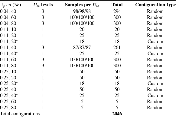


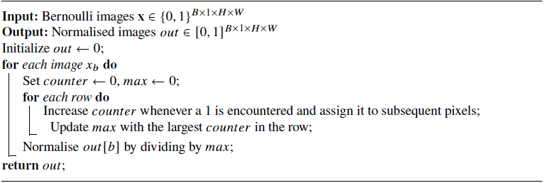
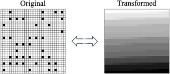
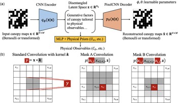


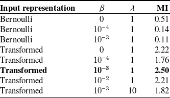

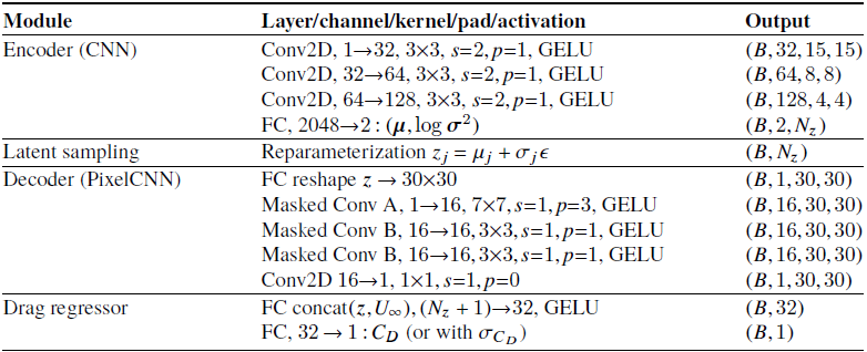


 Open access

