


1 Introduction
In the Netherlands, geothermal energy is regarded as a viable contribution to the required sustainable energy mix, and it is estimated that the total recoverable heat from sedimentary aquifers is 55 times larger than the Dutch annual heat consumption (Kramers et al., Reference Kramers, Van Wees, Pluymaekers, Kronimus and Boxem2012; Willems, Reference Willems2017). Because of this potential, the Dutch government wants to increase geothermal production to 50 PJ/a in 2030, which is equivalent to the annual heat consumption of 1 million Dutch households.
A good location for this increase in geothermal energy development is the West Netherlands Basin (WNB; Fig. 1A), which is densely populated, thereby having a high energy demand (Willems & Nick, Reference Willems and Nick2019). Furthermore, large amounts of energy are believed to be stored in the deep aquifer layers (Kramers et al., Reference Kramers, Van Wees, Pluymaekers, Kronimus and Boxem2012; Willems, Reference Willems2017). The WNB has also been heavily explored with regard to hydrocarbon production (e.g. Van Balen et al., Reference Van Balen, Van Bergen, De Leeuw, Pagnier, Simmelink, Van Wees and Verweij2000; Duin et al., Reference Duin, Doornenbal, Rijkers, Verbeek and Wong2006; Wong et al., Reference Wong, Batjes and de Jager2007; Kombrink et al., Reference Kombrink, Doornenbal, Duin, Den Dulk, Ten Veen and Witmans2012), making the regional geology and depth of the different aquifers well established (e.g. Duin et al., Reference Duin, Doornenbal, Rijkers, Verbeek and Wong2006; Pluymaekers et al., Reference Pluymaekers, Kramers, Van Wees, Kronimus, Nelskamp, Boxem and Bonté2012). Another reason why the WNB is attractive for geothermal energy development is that large quantities of geological and geophysical data (e.g. seismic data, well data and geological models) are freely available online (www.nlog.nl; e.g. Duin et al., Reference Duin, Doornenbal, Rijkers, Verbeek and Wong2006; Kombrink et al., Reference Kombrink, Doornenbal, Duin, Den Dulk, Ten Veen and Witmans2012; Pluymaekers et al., Reference Pluymaekers, Kramers, Van Wees, Kronimus, Nelskamp, Boxem and Bonté2012; Willems & Nick, Reference Willems and Nick2019).
(A) Map of the geothermal potential of the Netherlands. Black line highlights the extent of the Roer Valley Graben and West Netherlands Basin. (B) Expected temperature for the Triassic aquifers in the West Netherlands Basin (study area). Also note the location of different wells which have drilled the Lower Triassic formation and the extent of the 3D seismic volume used in this study (Fig. 3). The maps have been generated using ThermoGIS (www.thermogis.nl/; for additional details see Bonté et al., Reference Bonté, Van Wees and Verweij2012; Kramers et al., Reference Kramers, Van Wees, Pluymaekers, Kronimus and Boxem2012; Pluymaekers et al., Reference Pluymaekers, Kramers, Van Wees, Kronimus, Nelskamp, Boxem and Bonté2012; Van Wees et al., Reference Van Wees, Kronimus, Van Putten, Pluymaekers, Mijnlieff, Van Hooff and Kramers2012; Vrijlandt et al., Reference Vrijlandt, Struijk, Brunner, Veldkamp, Witmans, Maljers and Van Wees2019). Locations of the NLW-GT-01 and other wells targeting the Lower Triassic formation are also highlighted.

The WNB contains two aquifers which are generally considered as good candidates for heat extraction, namely: (1) the Nieuwerkerk Formation (Schieland group, Upper Jurassic to Lower Cretaceous) and (2) the Main Buntsandstein Group (Lower Triassic) (Kramers et al., Reference Kramers, Van Wees, Pluymaekers, Kronimus and Boxem2012). Up to 2018, 13 doublet systems have been realised in the WNB, with most wells targeting the Nieuwerkerk Formation, which generally shows good reservoir properties and doublet capacities (Willems & Nick, Reference Willems and Nick2019).
While most geothermal wells in the WNB target the Nieuwerkerk formation, the deeper-positioned Main Buntsandstein Subgroup (Volpriehausen, Detfurth and Hadsegsen) (Lower Triassic) is increasingly being recognised as a high-potential hot sedimentary aquifer, with expected temperatures ranging between 80°C and 140°C (Fig. 1B) (Kramers et al., Reference Kramers, Van Wees, Pluymaekers, Kronimus and Boxem2012). However, as a result of its relatively complex geological and diagenetic history, the Triassic is also regarded as a high-risk target. This is, for example, observed by multiple hydrocarbon exploration- and geothermal wells (e.g. BRIELLE-GT-01 & -02, RZB-01, BTL-01, MSG-01 & -02; Fig. 1B). The data from these wells show a wide variety of measured porosities and permeabilities (www.nlog.nl), with wells positioned at the basin fringe generally having better reservoir properties than wells located more towards the basin centre.
The complexity of the Lower Triassic was further exemplified by a recent geothermal exploration well (NLW-GT-01) which targeted the Triassic sandstones within the basin centre, anticipating temperatures surpassing 120°C (Fig. 1B). Although the test results showed temperatures of 120°C, the reservoir quality was much poorer than expected (i.e. porosity <5.0%, permeability <0.1 mD). Because of these poor reservoir properties, the NLW-GT-01 well was plugged and abandoned above the Triassic and the well is now actively producing from the more permeable Lower-Cretaceous Schieland group.
While showing poor reservoir quality, image logs and core samples taken from the NLW-GT-01 well did show that the targeted reservoir layers are heavily fractured, and multiple studies have shown that these natural features can significantly enhance the effective permeability of a normally tight rock, even under subsurface conditions (e.g. Nelson, Reference Nelson2001; Toublanc et al., Reference Toublanc, Renaud, Sylte, Clausen, Eiben and Nådland2005; Vidal & Genter, Reference Vidal and Genter2018; Holdsworth et al., Reference Holdsworth, Trice, Hardman, McCaffrey, Morton, Frei and Rogers2019). For this reason, the characterisation and modelling of natural fracture networks has become an integral component in predicting fluid flow patterns and the optimising of hydrocarbon production from structurally complex/tight reservoirs (e.g. Laubach et al., Reference Laubach, Lander, Criscenti, Anovitz, Urai, Pollyea and Pyrak-Nolte2019).
Natural fracture and fault systems are also known to influence/enhance geothermal heat production (e.g. Vidal et al., Reference Vidal, Genter and Chopin2017; Comerford et al., Reference Comerford, Fraser-Harris, Johnson and McDermott2018; Kushnir et al., Reference Kushnir, Heap and Baud2018). For example, in the Upper Rhine Graben most geothermal projects exploit heat which is stored in fluids positioned in large and connected fault and fracture networks (Vidal & Genter, Reference Vidal and Genter2018). Here, data from multiple geothermal wells targeting fractured intervals have shown that natural fractures/faults significantly enhance the effective permeability of normally impermeable basement rocks, making the production of heat possible (Schill et al., Reference Schill, Genter, Cuenot and Kohl2017; Vidal et al., Reference Vidal, Genter and Chopin2017; Vidal & Genter, Reference Vidal and Genter2018).
The aim of this study is to investigate and model the potential impact of natural fractures on geothermal heat extraction from the Main Bundsanstein Subgroup (Volpriehausen, Detfurth and Hadsegsen) targeted by the recently drilled NLW-GT-01 well (Fig. 1B). This is done by expanding upon seismic reservoir characterisation and Discrete Fracture Network (DFN) modelling methodologies commonly used in the petroleum industry. This study is structured as follows: First, the geological and structural setting of the study area are presented. Second, a reservoir-scale property model is generated using petrophysical data analysis and geostatistical seismic inversion. Third, the faults and fractures are characterised using image-log and core interpretation and seismic discontinuity analysis. Fourth, three reservoir-scale 2D DFNs are generated, using the acquired fracture/fault data and three different aperture models (power-law-, length-based and stress-based aperture). Fifth, the modelled DFNs, are upscaled to three fracture permeability models. Sixth, the acquired results are integrated into coupled fluid-flow and temperature simulations, such that the impact of natural fractures on geothermal heat extraction can be investigated. Finally, the implications of the results, modelling workflow and assumptions are discussed.
2 Geological and structural setting of the study area
2.1 Present-day geometry of the West Netherlands Basin
The WNB is located in the western part of the Netherlands and, together with the Roer Valley Graben (RVG) and Broad Fourteens Basin (BFB), forms a large failed rift system (Fig. 2A). From the Late Carboniferous onward, the WNB experienced several rifting (e.g. Triassic and Late Jurassic) and compression events (e.g. Alpine (Late Cretaceous to Early Tertiary)) (Van Balen et al., Reference Van Balen, Van Bergen, De Leeuw, Pagnier, Simmelink, Van Wees and Verweij2000; De Jager, Reference de Jager2007). The present-day geometry of the WNB is characterised by up to 5000 m of Permian to Tertiary deposits and a connected fault network of WNW–ESE to NNW–SSE-striking features (Worum et al., Reference Worum, Michon, Van Balen, Van Wees, Cloetingh and Pagnier2005; De Jager, Reference de Jager2007; Fig. 2A and B). In the Jurassic to Triassic levels, secondary faults striking N–S and E–W are also observed (De Jager, Reference de Jager2007). Due to the NNE–SSW Late-Cretaceous to Early-Tertiary compression events, most of the faults within the WNB have been inverted via dextral and sinistral transpression forming large inversion highs and positive flower structures at the base of the Cretaceous (e.g. Fig. 2B) (De Jager, Reference de Jager2007). Significant oil and gas accumulations, sourced by the Jurassic Posidonia Shale and Carboniferous coal layers, can be found within these inverted structures (De Jager et al., Reference de Jager, Doyle, Grantham, Mabillard, Rondeel, Batjes and Nieuwenhuijs1996; Van Balen et al., Reference Van Balen, Van Bergen, De Leeuw, Pagnier, Simmelink, Van Wees and Verweij2000). Additionally, these compression events resulted in significant uplift and erosion (down to the Jurassic near the inversion axis) (Fig. 2B; Van Balen et al., Reference Van Balen, Van Bergen, De Leeuw, Pagnier, Simmelink, Van Wees and Verweij2000).
(A) Map of the extent of the BFB, WNB and RVG within the Netherlands. Coordinates are in WGS 84. Basin geometry and faults after De Jager (Reference de Jager2007). The cross section (Fig. 2B) is depicted by the black line. (B) SSW–NNE cross section through the study area (WNB). Faults locations and geometry after Van Balen et al., (Reference Van Balen, Van Bergen, De Leeuw, Pagnier, Simmelink, Van Wees and Verweij2000). Cross section has been created using the DGM-deep model (Kombrink et al., Reference Kombrink, Doornenbal, Duin, Den Dulk, Ten Veen and Witmans2012). See for example Duin et al. (Reference Duin, Doornenbal, Rijkers, Verbeek and Wong2006) and Van Balen et al. (Reference Van Balen, Van Bergen, De Leeuw, Pagnier, Simmelink, Van Wees and Verweij2000) for details on the nomenclature and age of the different formations.

2.2 Stratigraphy and diagenesis of the Main Buntsandstein Subgroup (Early Triassic) in the WNB
The Main Buntsandstein Subgroup is composed of the Volprie-hausen, Detfurth and Hadsegsen formations. These formations were deposited under fluvial and aeolian conditions (palaeolatitude 20 to 25° N) and have a combined thickness ranging between 100 and 150 m (Geluk, Reference Geluk2005).
The Volpriehausen is generally subdivided into a lower and an upper part. The lower part comprises fluvial sandstones which were sourced from the London–Brabant Massif. Thicker and coarser-grained sandstones concentrate in the southern basin fringes (i.e. close to the London–Brabant Massif), with more distal parts being dominated by fine-grained sandstones and playa lake deposits (Geluk, Reference Geluk2005). The Upper Volpriehausen formation compriss a succession of lacustrine siltstones and claystones, with subordinate sandstone layers. The overlying Detfurth formation is relatively thin and is generally composed of sandstone layers followed by a succession dominated by claystones (Geluk, Reference Geluk2005). The Hardegsen formation is mainly composed of aeolian sand and siltstone deposits and generally shows good reservoir properties (Geluk, Reference Geluk2005).
The Main Buntsandstein Subgroup is characterised by two diagenetic events, the earliest of which occurred during or right after deposition. This diagenetic event mainly resulted in halite and anhydrite cementation, illite and clayey grain coating, and ferroan dolomitisation, and is believed to be related to the infiltration of meteoric waters (Purvis & Okkerman, Reference Purvis, Okkerman, Rondeel, Batjes and Nieuwenhuijs1996). This event was predominant in the Volpriehausen formation and generally resulted in a significant reduction of the initial porosity and permeability (i.e. depositional pore space became cemented) (Purvis & Okkerman, Reference Purvis, Okkerman, Rondeel, Batjes and Nieuwenhuijs1996). The second phase of diagenesis occurred during the main alpine inversion events (Late Cretaceous to Early Palaeogene), where areas which recorded strong exhumation experienced renewed surface conditions, causing the dissolution of the anhydrite and halite cements, and a general increase in the effective porosity and permeability of the Triassic formations (Matev, Reference Matev2011).
2.3 Previous reporting on the data extracted by NLW-GT-01
The data extracted by the NLW-GT-01 well have been extensively studied as part of the DESTRESS programme and most of the reporting is freely available (www.nlog.nl). Core analysis showed that primary porosities and permeabilities of the cored interval of the Main Buntsandstein Subgroup (Volpriehausen formation) are very poor, with measurements ranging from 1.4% to 3.9% and <0.001 mD to 0.02 mD, respectively. These poor properties are mainly attributed to the primary depositional texture (very fine sands), compaction and excessive cementation of dolomite, quartz and anhydrite. The measured porosities and permeabilities are similar to those of other wells targeting the Main Bundsandstein Subgroup in the northern part of the WNB (e.g. VAL-01, MKP-10, Q13-04-S1 and Q13-07-S2), which also showed significant reduction of primary properties due to cementation (Maniar, Reference Maniar2019). The presence of natural fractures is also reported. However, no definitive conclusions were reached on the conductivity of the observed structural features. Finally, due to gas infiltration and the poor reservoir properties, the decision was made to plug and abandon the NLW-GT-01 above the Triassic without performing a conventional well test.
2.4 Other mentions of natural fractures within the Lower Triassic formations of the WNB
Apart from the NLW-GT-01 well, other wells have also encountered fractured intervals within the Lower Triassic formations of the WNB. For instance, image-log and core data taken from the VAL-01 well showed significantly fractured intervals in proximity to a larger normal fault. In total, 288 closed and 22 partially open fractures were observed, and the interpreted features showed an overall NW–SE strike and dips ranging between 50° and 90°. Additionally, core photos taken from the PKP-01 well showed evidence of partially-open and non-cemented fractures being present within the Lower Triassic formations. Moreover, data from the P18-A-06 and Q13-07 wells indicated that reported mud losses could be attributed to fractured and faulted areas, which is a good indicator that these natural features locally enhance permeability (Matev, Reference Matev2011). However, while mentions of open fractures exist, most reported fractures are cemented or closed.
3 Data and methods
3.1 The dataset, velocity model and 2D modelling domain
This study focuses on the Triassic formations in the area surrounding the recently drilled NLW-GT-01 well (Figs 1 and 3). The main input data consist of reprocessed 3D seismic amplitude data, the VELOMOD-2 layer-cake velocity model, petrophysical wireline logs, a conductivity image log and 30 m of core data (Figs 3A and B and 4).
(A) Extent of the seismic crop, location of the NLW-GT-01 and the DE-LIER-45 wells and location of the modelling domain. See Figures 1B and 2B for additional information on the location of the seismic data within the WNB. (B) Composite line through the two wells. Here and in all subsequent figures, the coordinate system used is RD-Amersfoort (EPSG: 28992).

Overall workflow used in this study. The main steps involve (1) petrophysical analysis, (2) geostatistical inversion, (3) matrix property calculations, (4) fracture interpretation, (5) seismic discontinuity analysis, (6) DFN modelling and permeability upscaling, and (7) fluid flow and temperature modelling. See text for additional details on the input data and each analysis/modelling step.

The 3D seismic data are a reprocessed version of the 3D seismic volume L3NAM1990C and are available for research purposes upon request (courtesy of TNO) (Fig. 3). The reprocessing of the seismic data was done by the Nederlandse Aardolie Maatschappij (NAM) in 2011. To speed up the geophysical computations, we have cropped the seismic to the extent shown in Figure 3A.
For the velocity model, we use input data from VELOMOD-2, which is a statistical layer-cake model using all available well data and the main horizons within the Netherlands (van Dalfsen et al., Reference van Dalfsen, Doornenbal, Dortland and Gunnink2006, Reference van Dalfsen, Van Gessel and Doornenbal2007). In this study, the different interval velocities (
 $${v_{{\rm{int}}}}\left( {x,y,z} \right)$$
) for the main horizons within the WNB (see Fig. 2B) were calculated using:
$${v_{{\rm{int}}}}\left( {x,y,z} \right)$$
) for the main horizons within the WNB (see Fig. 2B) were calculated using:
 $${v_{{\rm{int}}\left( {\rm{i}} \right)}}\left( {x,y,z} \right) = {\rm{\;}}{v_{0\left( {\rm{i}} \right)}}\left( {x,y} \right) + {\rm{\;}}{k_{\left( {\rm{i}} \right)}}\left( {Z{{\left( {x,y} \right)}_{\left( {{\rm{i}} - 1} \right)}} + \frac{{{Z{{\left( {x,y} \right)}_{\left( {\rm{i}} \right)}} - {\rm{\;}}Z{{\left( {x,y} \right)}_{\left( {{\rm{i}} - 1} \right)}}}} \over {2}}} \right)}}$$
where
 $${v_{{\rm{int}}\left( {\rm{i}} \right)}}\left( {x,y,z} \right)$$
(m/s) is the interval velocity for layer i,
$${v_{{\rm{int}}\left( {\rm{i}} \right)}}\left( {x,y,z} \right)$$
(m/s) is the interval velocity for layer i,
 $${v_{0\left( {\rm{i}} \right)}}\left( {x,y} \right)$$
(m/s) is the initial velocity for layer i,
$${v_{0\left( {\rm{i}} \right)}}\left( {x,y} \right)$$
(m/s) is the initial velocity for layer i,
 $${k_{\left( {\rm{i}} \right)}}$$
(1/s) is the slope in the velocity increase with depth, and
$${k_{\left( {\rm{i}} \right)}}$$
(1/s) is the slope in the velocity increase with depth, and
 $$Z{\left( {x,y} \right)_{\left( {{\rm{i}} - 1} \right)}}$$
and
$$Z{\left( {x,y} \right)_{\left( {{\rm{i}} - 1} \right)}}$$
and
 $$Z{\left( {x,y} \right)_{\left( {\rm{i}} \right)}}$$
are the depth surfaces for layer i and the layer above. More information on the velocity model and the data used can be found in the Supplementary Material available online at https://doi.org/10.1017/njg.2020.21 or at www.nlog.nl/en/seismic-velocities.
$$Z{\left( {x,y} \right)_{\left( {\rm{i}} \right)}}$$
are the depth surfaces for layer i and the layer above. More information on the velocity model and the data used can be found in the Supplementary Material available online at https://doi.org/10.1017/njg.2020.21 or at www.nlog.nl/en/seismic-velocities.
Two wells which targeted the Main Buntsandstein Subgroup were used, namely NLW-GT-01 and DE-LIER-45 (Fig. 3). From the NLW-GT-01 well, wireline logs, the conductivity image log (FMI-8 Fullbore-formation-micro-imager (Schlumberger)) and core data were used for the petrophysical analysis, fracture interpretation and reservoir modelling. The depth of the different formations in the NLW-GT-01 well was based on the interpretation done by TNO in 2018 (Fig. 3B; see the Supplementary Material available online at https://doi.org/10.1017/njg.2020.21 or NLOG). The DE-LIER-45 well was used for wavelet extraction and synthetic seismic generation (see the Supplementary Material available online at https://doi.org/10.1017/njg.2020.21).
In this study, the reservoir property, DFN and temperature modelling domain is the area surrounding the NLW-GT-01 well (Fig. 3A). This 2D domain has grid dimensions of (dx = 1469 m, dy = 1371 m and z = 3940 m) and cell dimensions of 10 by 10 m. All modelling results (i.e. reservoir properties, DFNs and temperature/energy data) presented in this study will be constrained to this area.
3.2 General workflow and list of main processes, assumptions and uncertainties
The workflow and results presented in this study consist of three main parts:
-
1) Reservoir property (porosity and permeability) characterisation using (i) petrophysical wireline analysis, (ii) geostatistical inversion for acoustic properties and (iii) porosity and permeability computations for the modelling domain (Fig. 4; Table 1);
Table 1.Details of the process and main assumptions/uncertainties for each step in the workflow utilised in this study (Fig. 4). See text for additional information on each analysis- and modelling step.

-
2) Fracture/fault characterisation using (i) image-log and core interpretation and (ii) seismic attribute analysis (Fig. 4; Table 1);
-
3) Assessment of the impact of natural fractures on geothermal heat extraction from the Lower Triassic successions, using: (i) DFN modelling, (ii) fracture aperture modelling using three different scenarios, (iii) permeability upscaling and (iv) fluid flow and temperature modelling (Fig. 4; Table 1).

Additional information on the main processes, assumptions and uncertainties used within the presented workflow can be found in Table 1.
3.3 Petrophysical analysis
Petrophysical logs (bulk/grain density, S- and P-sonic-velocities, gamma ray and effective porosity (HILT)) from the two wells (NLW-GT-01 and DE-LIER-45) were taken from the Dutch repository for subsurface data (www.nlog.nl). From these different wireline logs, the P- and S-impedance, P- and S-velocity and the total and effective porosity were computed. These different datasets were then used for (i) finding correlations between the different elastic and reservoir properties, (ii) creating a representative wavelet and synthetic seismics, (iii) well-to-seismic correlations and (iv) geostatistical inversion (Fig. 4; Table 1). More information on the computations and results can be found in the Supplementary Material available online at https://doi.org/10.1017/njg.2020.21.
3.4 Geostatistical inversion and property modelling
The seismic and well data were integrated using geostatistical inversion, which allows for the generation of high-frequency property models (McCrank et al., Reference McCrank, Lawton and Mangat2009; Delbecq & Moyen, Reference Delbecq and Moyen2010; Fig. 4; Table 1). The tool used in this study was the StatMod package in Jason (developed by CGG). This tool uses (1) statistical functions (probability density functions and variograms) describing the petrophysical properties observed within wells, (2) a tailored seismic wavelet, (3) seismic amplitude data (in TWT), (4) wavelet deconvolution, (5) Bayesian interference and (6) a Markov chain Monte Carlo sampling algorithm (e.g. Sams et al., Reference Sams, Millar, Satriawan, Saussus and Bhattacharyya2011), in order to statistically invert seismic amplitude data to different acoustic and/or petrophysical properties (e.g. acoustic impedance or rock density) (Fig. 4; Table 2). The StatMod algorithm also aims at honouring the well and seismic data by minimising the residual between the modelled synthetic and the original seismic data.
Constant parameters used for each simulation

In this study, we inverted for the acoustic impedance using the time-converted post-stacked seismic-amplitude data, extracted wavelet and computed P-impedance wireline log (see the Supplementary Material available online at https://doi.org/10.1017/njg.2020.21). The model had lateral grid dimensions equal to the seismic voxel spacing (i.e. 20 by 20 m). The vertical spacing was set at 0.5 ms, so that detailed petrophysical changes could be incorporated in the geostatistical inversion workflow. The NLW-GT-01 input well was assumed to be ‘blind’, so that the petrophysical well data were only used as statistical input and not as hard constraining data. For the presented results, the input settings and statistical functions were tailored, so that the match between the inverted results, blind well data and original seismic data had a qualitative fit and no large discrepancies. See the Supplementary Material available online at https://doi.org/10.1017/njg.2020.21 for more information on the used settings.
From the inverted impedance data, the porosity (effective and total) and density were computed using the relations determined from the petrophysical analysis (Fig. 4; Table 1). The effective and total porosities were then used to calculate the matrix permeability within the modelling domain using measurements from a core hot shot analysis done on the NLW-GT-01 core (measurements done by Panterra; report is available on NLOG):
 $${\rm{ln}}\left( {{K_{{\rm{mat}}}}} \right) = C + D\varphi $$
where C and D are constants and are set at −2.512 and 0.233, respectively.
 $${K_{{\rm{mat}}}}$$
is the computed matrix permeability (Md).
$${K_{{\rm{mat}}}}$$
is the computed matrix permeability (Md).
 $$\varphi $$
is the porosity (effective or total; %).
$$\varphi $$
is the porosity (effective or total; %).
3.5 Borehole image-log and core interpretation and fracture characterisation
The aforementioned conductivity image log of the NLW-GT-01 well was interpreted using Schlumberger’s wellbore software program Techlog (Techlog ®). The image log has a total length of 192 m (MD: 4190 m to MD: 4382 m), covering the full Volpriehausen formation and parts of the Detfurth and Rogenstein formations (Rogenstein underlies the Volrpiehausen). Apart from the image log, 30 m of core (MD: 4250 m to MD: 4280 m) was analysed and interpreted using PanTerra’s core interpretation tool (Electronic Core Goniometry ®) (for the interpretation see the Supplementary Material available online at https://doi.org/10.1017/njg.2020.21).
On the image log, fracture planes were interpreted as features showing a distinct sinusoid shape and an increase in conductivity with respect to the surrounding rock matrix. Furthermore, the interpretation was guided by the resistivity log and the available core interpretation. One distinct characteristic of the NLW-GT-01 well data is that the conductivity image log shows much more interpretable discontinuities than core data (for the same interval). These additional discontinuities observed within the FMI data have been interpreted as being hydraulically- or drilling-induced fractures. For this reason, we have interpreted the image log using a very conservative methodology. This implies that only features which were visible in the core or show a full sinusoid were interpreted.
From the interpreted data, the fracture intensity (P21) along the NLW-GT-01 well was calculated using two different sampling windows of 2.5 m and 10 m, respectively. The larger sampling window was chosen to compare the interpreted fracture intensity to discontinuities observed in the seismic signal.
Characteristics such as height, length and aperture were calculated for all the interpreted fractures. The fracture length was calculated from the computed heights, assuming a constant aspect ratio (length/height) of 4.0, which is commonly observed in outcrop analogues (e.g. Schultz & Fossen, Reference Schultz and Fossen2002). However, it should be noted that assigning a constant aspect ratio is a significant assumption which may introduce non-representative results (Table 1). Fracture aperture computation requires image logs to be calibrated, which for this study was done using the mud resistivity and by manually fitting a calibration curve (for additional information see the Supplementary Material available online at https://doi.org/10.1017/njg.2020.21 and the Techlog user documentation). From the calibrated data, the fracture width was calculated using the aperture equation proposed by Luthi & Souhaite (Reference Luthi and Souhaite1990):
 $$W = cAR_{\rm{m}}^bR_{x0}^{1 - b}$$
where W is the fracture width (mm) at each location along the fracture, A is excess current which can be injected into the formation divided by the voltage,
 $${R_{x0}}$$
is the formation resistivity,
$${R_{x0}}$$
is the formation resistivity,
 $${R_{\rm{m}}}$$
is the mud resistivity, and c and b are tool-specific and numerically derived values (for FMI-8:
$${R_{\rm{m}}}$$
is the mud resistivity, and c and b are tool-specific and numerically derived values (for FMI-8:
 $$c = 0.004801\;{\rm{\mu m}}$$
,
$$c = 0.004801\;{\rm{\mu m}}$$
,
 $$b = 0.863$$
) (Luthi & Souhaite, Reference Luthi and Souhaite1990). From the fracture width (W) the mean and hydraulic aperture were calculated using the standard settings in Techlog (see Techlog user documentation for additional information).
$$b = 0.863$$
) (Luthi & Souhaite, Reference Luthi and Souhaite1990). From the fracture width (W) the mean and hydraulic aperture were calculated using the standard settings in Techlog (see Techlog user documentation for additional information).
3.6 Seismic discontinuity analysis
Discontinuities detectable on the reprocessed seismic (Fig. 5A) were automatically extracted using three volume attributes available in OpendTect (OpendTect ®). The extracted seismic discontinuities were subsequently used as input for our DFN models (Fig. 4; Table 1).
Fault cube extraction workflow using OpendTect 6.0.0. (A) Original seismic data. (B) Similarity cube extracted from the Fault Enhancement Filtered (FEF) seismic data. (C) Fault Likelihood (FLH) cube extracted from the FEF seismic data. For additional information see text and Jaglan & Qayyum (Reference Jaglan and Qayyum2015) and Hale (Reference Hale2013). There is no vertical exaggeration in the figure.

The first step in the presented attribute analysis was to ‘enhance’ the original seismic data for discontinuity analysis using a collection of subsequent volume attributes collectively called the Fault Enhancement Filter (FEF; Jaglan & Qayyum, Reference Jaglan and Qayyum2015). This filter smooths seismic data which have a ‘clean’ signal and sharpens seismic data with a distorted signal, essentially enhancing faulted areas.
From the FEF seismic cube, the similarity attribute was computed (Fig. 5B). This attribute has values ranging between 0 and 1, with clean seismic data having values close to 1, and distorted seismic data having lower values (Fig. 5B). This attribute is commonly used for characterising seismic discontinuities (e.g. Jaglan & Qayyum, Reference Jaglan and Qayyum2015). In this study, the similarity attribute cube (Fig. 5B) was used as input for populating the fracture intensity in the modelling domain.
The FEF seismic cube was also used as input for the Thinned-Fault-Likelihood (TFL) attribute, which has been developed by Hale (Reference Hale2013) and implemented in OpendTect (Jaglan & Qayyum, Reference Jaglan and Qayyum2015). The TFL attribute highlights areas which show a distorted seismic amplitude signal (i.e.
 $${\rm{TFL}} = {\left( {1 - {\rm{semblance}}} \right)^8}$$
), with semblance being representative for the continuity in the seismic signal. We used this attribute to thin and enhance areas which show sharp changes in the seismic data, along user-defined dip- and dip-azimuth ranges (dip range of 45–85 and azimuth range of 0–360) (Fig. 5c). The resulting TFL attribute forms the fault cube which is further utilised in the DFN modelling workflow (Fig. 4; Table 1).
$${\rm{TFL}} = {\left( {1 - {\rm{semblance}}} \right)^8}$$
), with semblance being representative for the continuity in the seismic signal. We used this attribute to thin and enhance areas which show sharp changes in the seismic data, along user-defined dip- and dip-azimuth ranges (dip range of 45–85 and azimuth range of 0–360) (Fig. 5c). The resulting TFL attribute forms the fault cube which is further utilised in the DFN modelling workflow (Fig. 4; Table 1).
3.7 Discrete Fracture Network (DFN), aperture and permeability modelling
The 2D DFN in the modelling domain was populated by implementing (1) the interpreted fracture data from the available image logs and (2) the results of the seismic discontinuity analysis (Figs 4 and 5; Table 1) into the Petrel fracture network modelling workflow.
First, the fracture intensity map was based on the inverse similarity map (1 − seismic similarity) and the correlation between fracture intensity and similarity (Fig. 4;Table 1). Second, the local fracture orientation was assumed to be parallel to the faults within the modelling domain (i.e. fault-related fracturing). To this end, the local fracture orientation was based on a linearly interpolated map of the measured seismic fault orientation (observed on the TFL cube) within the modelling domain (Fig. 4; Table 1). Lastly, the spread in local fracture orientation was modelled using a constant Fisher coefficient (Fisher, Reference Fisher1953), which was derived from the observed standard deviation in fracture orientation.
To model the aperture on each fracture within the DFN, we have created three different scenarios: (1) measured aperture, (2) length-based aperture and (3) mechanical aperture. These three aperture models were chosen so that potential differences in fracture characteristics are adequately captured and depicted. However, we do acknowledge that the full range of potential uncertainties involved in modelling fracture aperture cannot be described by only using three different models.
In the first scenario, aperture was based on observations from the image-log data (Section 4.2.1). The observed aperture data were used to create a probability density function which was in turn used to populate the aperture on each fracture in the DFN.
For the second scenario, we assumed that fracture length and aperture are related via an often observed sub-linear scaling law (e.g. Vermilye & Scholz, Reference Vermilye and Scholz1995; Olson, Reference Olson2003), so that the fracture aperture can be calculated using:
 $${e_{\rm{l}}} = C{L^a}$$
where
 $${e_{\rm{l}}}$$
is the modelled length-based fracture aperture (m), C is the pre-exponential constant, which was set at
$${e_{\rm{l}}}$$
is the modelled length-based fracture aperture (m), C is the pre-exponential constant, which was set at
 $$5.0 \cdot {10^{ - 5}}$$
, L is the total fracture length (m), and a is the power-law scaling exponent which was set at 0.5.
$$5.0 \cdot {10^{ - 5}}$$
, L is the total fracture length (m), and a is the power-law scaling exponent which was set at 0.5.
For the third scenario, we used the mechanical aperture model first defined by Barton & Bandis (Reference Barton and Bandis1980). This model uses empirical relationships to describe mechanical closure of initially open fractures due to an applied normal stress (e.g. Asadollahi & Tonon, Reference Asadollahi and Tonon2010; Bisdom et al., Reference Bisdom, Bertotti and Nick2016, Reference Bisdom, Nick and Bertotti2017b; Boersma et al., Reference Boersma, Prabhakaran, Bezerra and Bertotti2019). This closure can be described by a hyperbolic function so that the mechanical aperture follows:
 $${e_{\rm{n}}} = {e_0} - {\left( {\frac{{1}\ \over {{{v_{\rm{m}}}}}} + \;\frac{{{{K_{{\rm{ni}}}}}} \over{{{\sigma _{\rm{n}}}}}}} \right)^{ - 1}}$$
where
 $${e_{\rm{n}}}$$
is the resulting mechanical aperture (mm),
$${e_{\rm{n}}}$$
is the resulting mechanical aperture (mm),
 $${e_0}$$
is the initial fracture aperture (mm),
$${e_0}$$
is the initial fracture aperture (mm),
 $${v_{\rm{m}}}$$
is the maximum closure (mm),
$${v_{\rm{m}}}$$
is the maximum closure (mm),
 $${K_{{\rm{ni}}}}$$
is the fracture stiffness, and
$${K_{{\rm{ni}}}}$$
is the fracture stiffness, and
 $${\sigma _{\rm{n}}}$$
is the normal stress on the fracture plane (Barton & Bandis, Reference Barton and Bandis1980). The maximum closure (
$${\sigma _{\rm{n}}}$$
is the normal stress on the fracture plane (Barton & Bandis, Reference Barton and Bandis1980). The maximum closure (
 $${v_{\rm{m}}}$$
) and stiffness (
$${v_{\rm{m}}}$$
) and stiffness (
 $${K_{{\rm{ni}}}}$$
) are empirically measurable material parameters, which depend on the joint roughness coefficient (JRC) and the joint compressive strength (JCS) of each fracture plane (Asadollahi, Reference Asadollahi2009). In this study, we assumed that the modelled fractures are irregular and have a JRC of 7.5 and JCS of 17.5 (MPa), so that
$${K_{{\rm{ni}}}}$$
) are empirically measurable material parameters, which depend on the joint roughness coefficient (JRC) and the joint compressive strength (JCS) of each fracture plane (Asadollahi, Reference Asadollahi2009). In this study, we assumed that the modelled fractures are irregular and have a JRC of 7.5 and JCS of 17.5 (MPa), so that
 $${v_{\rm{m}}}$$
and
$${v_{\rm{m}}}$$
and
 $${K_{{\rm{ni}}}}$$
are equated as (Asadollahi, Reference Asadollahi2009; Bisdom et al., Reference Bisdom, Bertotti and Nick2016a):
$${K_{{\rm{ni}}}}$$
are equated as (Asadollahi, Reference Asadollahi2009; Bisdom et al., Reference Bisdom, Bertotti and Nick2016a):
 $${v_{\rm{m}}} = - 0.1032 - 0.0074{\rm{JRC}} + 1.135{\left( {\frac{{{\rm{JCS}}}} \over {{{e_0}}}} \right)^{ - 0.251}}$$
 $${K_{{\rm{ni}}}} = - 7.15 + 1.75{\rm{JRC}} + 0.02\frac{{{{\rm{JCS}}}} \over {{{e_0}}}}$$
For all scenarios, the modelled aperture was translated to a permeability on each fracture plane, using the parallel plate law):
 $${K_{{\rm{frac}}}} = \frac{{{{e^2}}} \over {{12}}}$$
where e is the respective fracture aperture (m) and
 $${K_{{\rm{frac}}}}$$
is the fracture permeability (m2).
$${K_{{\rm{frac}}}}$$
is the fracture permeability (m2).
Finally, the
 $${K_{{\rm{frac}}}}$$
on each fracture in the DFN was upscaled to an effective fracture permeability for respective grid cell using the Oda method. This method assumes that individual fractures within a grid cell can be upscaled to an effective crack (permeability) tensor using geometrical statistics (i.e. fracture orientation, fracture trace length and fracture permeability) (Oda, Reference Oda1985). In total, three upscaled fracture permeability models based on the different aperture models were created (i.e. power-law aperture (measured), length-based aperture and stress-based aperture).
$${K_{{\rm{frac}}}}$$
on each fracture in the DFN was upscaled to an effective fracture permeability for respective grid cell using the Oda method. This method assumes that individual fractures within a grid cell can be upscaled to an effective crack (permeability) tensor using geometrical statistics (i.e. fracture orientation, fracture trace length and fracture permeability) (Oda, Reference Oda1985). In total, three upscaled fracture permeability models based on the different aperture models were created (i.e. power-law aperture (measured), length-based aperture and stress-based aperture).
3.8 Fluid-flow/temperature modelling
Fluid and temperature simulations were done using the Delft Advanced Research Terra Simulator (DARTS), which is a python/C++ based simulator capable of simulating high-enthalpy (water and steam) systems (Khait, Reference Khait2019; Wang et al., Reference Wang, Voskov, Khait and Bruhn2020) (Fig. 4; Table 1). DARTS assumes that the two-phase thermal system can be described by mass and energy conservation equations (Wang et al., Reference Wang, Voskov, Khait and Bruhn2020):
 $$\frac{{\partial } \over {{\partial t}}}\left( {\varphi \mathop \sum \nolimits_{p = 1}^{{n_p}} {\rho _p}{s_p}} \right) - {\rm{div}}\mathop \sum \nolimits_{p = 1}^{{n_p}} {\rho _p}{u_p} + \;\mathop \sum \nolimits_{p = 1}^{{n_p}} {\rho _p}{q_p} = 0,$$
 $$\frac{{\partial } \over {{\partial t}}}\left( {\varphi \mathop \sum \nolimits_{p = 1}^{{n_p}} {\rho _p}{s_p}{U_p} + \left( {1 - \varphi } \right){U_r}} \right) - {\rm{div}}\mathop \sum \nolimits_{p = 1}^{{n_p}} {h_p}{\rho _p}{u_p} + \;{{\rm{div}}\left( {\kappa \nabla T} \right) + \mathop \sum \nolimits_{p = 1}^{{n_p}} {h_p}{\rho _p}{q_p} = 0}$$
where
 $$\;p$$
is the phase (
$$\;p$$
is the phase (
 $$p = 1$$
(water) and
$$p = 1$$
(water) and
 $$p = $$
2 (vapour)),
$$p = $$
2 (vapour)),
 $$\varphi $$
is the porosity,
$$\varphi $$
is the porosity,
 $${s_p}$$
is the phase saturation (
$${s_p}$$
is the phase saturation (
 $${s_1}$$
+
$${s_1}$$
+
 $${s_2}$$
= 1.0),
$${s_2}$$
= 1.0),
 $${\rho _p}$$
is the phase density (kg/m3),
$${\rho _p}$$
is the phase density (kg/m3),
 $${U_p}$$
is the phase internal energy (kJ),
$${U_p}$$
is the phase internal energy (kJ),
 $${U_r}$$
is the rock internal energy (kJ),
$${U_r}$$
is the rock internal energy (kJ),
 $${h_p}$$
is the phase enthalpy (kJ/kg),
$${h_p}$$
is the phase enthalpy (kJ/kg),
 $$\kappa $$
is the thermal conduction (kJ/m/day/K), T is the temperature (K),
$$\kappa $$
is the thermal conduction (kJ/m/day/K), T is the temperature (K),
 $${u_p}$$
is the phase velocity (m/s) and
$${u_p}$$
is the phase velocity (m/s) and
 $${q_p}$$
is the phase mass-flow rate (m3/s).
$${q_p}$$
is the phase mass-flow rate (m3/s).
Fluid flow is described using Darcy’s law:
 $${q_p} = K\frac{{{{k_{rp}}}} \over {{{\mu _p}}}}\left( {\nabla {P_p} - {\gamma _p}D} \right)$$
where
 $${q_p}$$
is the mass flow rate for phase p (m3/s), K is the permeability matrix (mD),
$${q_p}$$
is the mass flow rate for phase p (m3/s), K is the permeability matrix (mD),
 $${k_{rp}}$$
is the relative permeability for phase p (mD),
$${k_{rp}}$$
is the relative permeability for phase p (mD),
 $${\mu _p}$$
is the phase viscosity,
$${\mu _p}$$
is the phase viscosity,
 $${P_p}$$
is the pressure for phase
$${P_p}$$
is the pressure for phase
 $$\;p$$
,
$$\;p$$
,
 $${\gamma _p}$$
is the phase specific weight (N/m3) and D is the depth (m).
$${\gamma _p}$$
is the phase specific weight (N/m3) and D is the depth (m).
To assess the impact that fractures could have on geothermal heat production, the computed matrix properties and upscaled fracture permeability models (one for each aperture scenario) were used to create four different simulation scenarios. These scenarios will be explained in more detail in the results section (Section 4).
For each scenario, one injector and one producer well were placed vertically in two cells showing a relatively high fracture intensity which are spaced 780 m apart. Fluid flow was initiated by creating a bottom-hole pressure difference between injector and producer (injector BHP = 375 bar, producer BHP = 425 bar). The injection temperature was set at 30.0°C. The initial reservoir temperature and pressure were set at 120°C and 400 bar, respectively (Table 2). Simulation run time was set at 30 years. Finally, the model was assumed to be a closed system, implying that no flow in/out of the model boundaries was possible. See Table 2 for the rest of the initial conditions.
4 Results
4.1 Petrophysical analysis, geostatistical inversion, and property computations in the modelling domain
4.1.1 Petrophysical analysis of the NLW-GT-01 well
The available wireline logs cover the Main Buntsandstein formations (Fig. 6A). The Hardegsen and Detfurth formations show a relatively low density (
 $$\rho = 2.58\; \pm 0.056$$
g/cm3), P- and S-velocity (
$$\rho = 2.58\; \pm 0.056$$
g/cm3), P- and S-velocity (
 $${V_P} = 4782.32\; \pm 241.12$$
m/s and
$${V_P} = 4782.32\; \pm 241.12$$
m/s and
 $${V_s} = 3035.63\; \pm 14.851$$
m/s) and low P- and S-impedance (
$${V_s} = 3035.63\; \pm 14.851$$
m/s) and low P- and S-impedance (
 $${I_P} = 12376.10\; \pm 839.59$$
(g/cm3)(m/s) and
$${I_P} = 12376.10\; \pm 839.59$$
(g/cm3)(m/s) and
 $${I_s} = 7853.33\; \pm 498.586$$
(g/cm3)(m/s)) (Fig. 6A). The measured effective and total porosities are relatively high (compared to the rest of the data) (
$${I_s} = 7853.33\; \pm 498.586$$
(g/cm3)(m/s)) (Fig. 6A). The measured effective and total porosities are relatively high (compared to the rest of the data) (
 $${\varphi _{{\rm{eff}}}} = 0.028\; \pm 0.013,$$
 $${\varphi _{{\rm{tot}}}} = 0.057\; \pm 0.02$$
) (Fig. 6A). The Volpriehausen formation shows higher density and P- and S-velocity and lower P- and S-impedance values, with respect to the Detfurth and Hardegsen formations (Fig. 6A). Additionally, the petrophysical analysis indicates that the Volpriehausen formation has almost no intrinsic porosity (i.e.
$${\varphi _{{\rm{tot}}}} = 0.057\; \pm 0.02$$
) (Fig. 6A). The Volpriehausen formation shows higher density and P- and S-velocity and lower P- and S-impedance values, with respect to the Detfurth and Hardegsen formations (Fig. 6A). Additionally, the petrophysical analysis indicates that the Volpriehausen formation has almost no intrinsic porosity (i.e.
 $${\varphi _{{\rm{eff}}}} = 0.010\; \pm 0.006$$
and
$${\varphi _{{\rm{eff}}}} = 0.010\; \pm 0.006$$
and
 $${\varphi _{{\rm{tot}}}}\;0.022\; \pm 0.012$$
) (Fig. 6A). These lower porosities were also observed in core plug measurements, and are believed to be caused by the primary depositional environment, compaction and different diagenetic events (i.e. dolomite, quartz and anhydrite cementation) (www.nlog.nl).
$${\varphi _{{\rm{tot}}}}\;0.022\; \pm 0.012$$
) (Fig. 6A). These lower porosities were also observed in core plug measurements, and are believed to be caused by the primary depositional environment, compaction and different diagenetic events (i.e. dolomite, quartz and anhydrite cementation) (www.nlog.nl).
Petrophysical analysis of the NLW-GT-01 well. (A) From left to right: gamma ray, density, P- and S-velocity, P- and S-impedance and total and effective porosity logs. (B) Measured/calculated porosity vs the measured density. (C) Porosity vs the P-impedance. (D) Rock density vs the P-impedance. Note that the different relations are depicted at the bottom of (B), (C) and (D), respectively.

Linear regression analysis indicates that the different petrophysical properties can be related (Fig. 6B–D). The results show that rock density vs effective and total porosity follows a negative-exponential and negative-linear relation, respectively (Fig. 6B). The effective and total porosity vs acoustic impedance (
 $${I_P}$$
) also shows a negative-exponential and negative-linear relationship (Fig. 6c). The density and acoustic impedance follow a negative-linear relationship (Fig. 6D).
$${I_P}$$
) also shows a negative-exponential and negative-linear relationship (Fig. 6c). The density and acoustic impedance follow a negative-linear relationship (Fig. 6D).
4.1.2. Geostatistical inversion and property modelling
The geostatistical inversion results show that relatively low acoustic impedance values occur in areas where there is a distinct change from positive to negative amplitude (Fig. 7A and B). Our results also indicate that areas showing low acoustic impedance correlate very well with the more porous portions of the Hardegsen and Detfurth formations (Fig. 7A–C). This is for example seen in the NLW-GT-01 well which goes through a succession with relatively low acoustic impedance values that coincide with the Hardegsen and Detfurth formations (Fig. 7A–C).
(A–B) Inline through the seismic amplitude data and inverted acoustic impedance data at the NLW-GT-01 location. (C) Porosity and P-impedance well logs, inverted seismic properties and the depth-converted seismic data extracted along the NLW-GT-01 well. Note that small discrepancies between the inverted data and well logs likely exist due to uncertainties in the velocity model.

Using the relations extracted from the petrophysical analysis (Fig. 6), the inverted acoustic impedance is converted to a total and effective porosity. The resulting properties show a good correlation with the porosity data observed in the NLW-GT-01 well (Figs 6 and 7C). However, some discrepancies between the well and seismic data exist. For instance, the peaks in porosity observed from the wireline data do not completely overlap with peaks detected within the properties calculated from seismic inversion (Fig. 7C). These differences could be explained by the uncertainties in the velocity model which has been used in the seismic inversion workflow (Section 3.1; Supplementary Material available online at https://doi.org/10.1017/njg.2020.21; Van Dalfsen et al., Reference van Dalfsen, Doornenbal, Dortland and Gunnink2006, Reference van Dalfsen, Van Gessel and Doornenbal2007), or uncertainties in the reprocessing of the seismic data.
Within the 2D modelling domain, changes in seismic amplitude coincide with changes in the acoustic impedance and computed porosities (Fig. 8A–D). Because the data are depicted on a z-slice (z = 3940 m), the stark changes in the seismic properties correspond to changes in the rock properties (i.e. Hardegsen/Detfurth = low
 $${I_P}$$
and (relatively) high
$${I_P}$$
and (relatively) high
 $$\varphi $$
and Volpriehausen = high
$$\varphi $$
and Volpriehausen = high
 $${I_P}$$
and low
$${I_P}$$
and low
 $$\varphi $$
) (Fig. 8A–D). Using equation 2, the total and effective porosities (Fig. 8C–D) are converted to a total and effective permeability (Fig. 8E–F). For the total permeability field, the computed values range between 0.072 mD, for the areas showing low porosities and 1.95 mD for areas showing high porosities (Fig. 8E). The effective permeability values range between 0.077 and 0.46 mD (Fig. 8F).
$$\varphi $$
) (Fig. 8A–D). Using equation 2, the total and effective porosities (Fig. 8C–D) are converted to a total and effective permeability (Fig. 8E–F). For the total permeability field, the computed values range between 0.072 mD, for the areas showing low porosities and 1.95 mD for areas showing high porosities (Fig. 8E). The effective permeability values range between 0.077 and 0.46 mD (Fig. 8F).
(A–B) Seismic amplitude and inverted impedance within the modelling domain. (C–D) Modelled total and effective porosity within the modelling domain. (E) Permeability map calculated from the total porosity. (F) Permeability field calculated from the effective porosity (HILT Porosity). The relation between porosity and permeability was from the core hot shots measurements done by Panterra (equation 2, Section 3.4) (www.nlog.nl).

4.2 Fracture and fault network characterisation
4.2.1 FMI and core interpretation and fracture analysis
Using the conservative interpretation method explained in Section 3.5, a total of 58 fractures have been interpreted, which is 6.7% of the observed conductive features in the image-log data. The resulting interpretation shows that fractures and faults mainly occur in clustered intervals within the Volpriehausen formation (Fig. 9A), with an average intensity (P10) of 0.53 (1/m) (Fig. 9A). Fractures and faults show a relative increase in the conductivity image log, implying that they are conductive and have a measurable aperture (Fig. 9B). All interpreted features strike NW–SE and have dips ranging between 60° and 90° (faults approximately 60° and fractures approximately 85°) (Fig. 9C). The observed NW–SE strike is parallel to the main faults in the WNB. The image log and core interpretations also highlight that faults which show minor displacement (mm to cm scale) of the bedding planes have been sampled by the NLW-GT-01 well (Fig. 9B and D). The fractures/faults observed in the cored interval show a similar NW–SE strike with measured dips ranging between 45° and 90° (Fig. 9E).
Structural fracture data extracted from the FMI and core data. (A) Fault and fracture intensity (P10) and gamma ray log for the entire NLW-GT-01 well. (B) Two examples of large fractures interpreted from the FMI data. (C) Rose- and stereodiagram depicting the orientation distribution for all interpreted fractures and faults from the FMI image data. (D) Example of faults and fractures observed within the cored interval of NLW-GT-01 well. Note that Figure 8B (left and right) represents the same intervals, respectively. (E) Measured fracture orientation observed from the core data.

By calibrating the conductivity image log (Fig. 9), the mean and hydraulic aperture of the interpreted fractures can be calculated (see Section 3.5). The results show that all fractures are more conductive than the surrounding rock matrix, with some large fractures in the lower part of the Volpriehausen formation showing a distinct reduction in the calibrated resistivity log (Fig. 10). This is also indicated by the computed fracture apertures, which show that most fractures have a hydraulic and mean aperture ranging between 0.01 mm and 0.10 mm (Fig. 10). Highly conductive features have an aperture ranging between 0.10 mm and 0.42 mm (Fig. 10). Due to crumbling of the core near open fractures, the computed apertures could not be validated against core measurements (Fig. 9D). Nonetheless, these results imply that the fractures are at least partly open and most likely enhance the effective permeability of the normally tight Volpriehausen sandstones.
Calibrated FMI log and fracture aperture results for the Upper and Lower Volplriehausen, respectively. Note that fractures are more conductive than the surrounding reservoir rock.

The measured fracture aperture distribution shows negative power-law behaviour (Fig. 11A), which can best be described by:
 $$P\left( {e;a,\;b} \right) = b \cdot {e^{ - a}}$$
(A) Histogram and power-law fit through the hydraulic apertures. (B) Normalised frequency of the fracture length taken from the FMI and log-normal function fitting the data. The fracture length is calculated from the measured fracture height (
 $${\rm{Length}} = 4 \cdot {\rm{Dip\;Height}}$$
).
$${\rm{Length}} = 4 \cdot {\rm{Dip\;Height}}$$
).

where e is the fracture aperture (mm) and a and b are the power-law exponent and scaling factor which are fitted at 1.543 and 0.191, respectively (Fig. 10A).
The computed fracture lengths range between 0 m and 12 m (Fig. 11B). The frequency distribution highlights that the fracture lengths can best be described by a log-normal function:
 $$P\left( {\ln l;\;\mu ,\;\sigma } \right) = \frac{{1} \over {{\sigma \sqrt {2\pi} } }}{\rm{exp}}\left[ {\frac{{{{\left( {\ln l - \mu } \right)}^2}}} \over{{2{\sigma ^2}}}} \right],\;l & #38; gt; \;0$$
where l is the fracture length (m),
 $$\mu $$
is proportional to the median (set at 0.2) and
$$\mu $$
is proportional to the median (set at 0.2) and
 $$\sigma $$
is proportional to the variance in the data and is set at 0.6 (Fig. 10b). The extracted probability density function (equations 12 and 13) will be used as input parameters for the DFN modelling workflow (Sections 4.3.1 and 4.3.2).
$$\sigma $$
is proportional to the variance in the data and is set at 0.6 (Fig. 10b). The extracted probability density function (equations 12 and 13) will be used as input parameters for the DFN modelling workflow (Sections 4.3.1 and 4.3.2).
4.2.2 Automated fault extraction and characterisation
At 3940 m depth, the TFL cube shows that faults have a dominant orientation striking NW–SE to N–S and are mainly aligned along the inverted horst structures (Fig. 12A). The extracted faults are largely consistent with previous fault interpretations within the WNB (e.g. Van Balen et al., Reference Van Balen, Van Bergen, De Leeuw, Pagnier, Simmelink, Van Wees and Verweij2000; De Jager, Reference de Jager2007).
Extracted fault cube data. (A) Z-slice at 3904 m depth (at Triassic interval near-reservoir target) showing the extracted Triassic faults, modelling domain, well location and the location of the cross section (Fig. 11B). Note that the z-slice has been rotated 38.59° with respect to the north. (B) NE–SW cross section through the 3D seismic and fault cube. (C) Faults extracted within the modelling domain.

At the Triassic/Jurassic intervals (±2800–3800 m), the extracted faults show both normal - and reverse displacement. The larger faults follow the dominant NW–SE to N–S strikes and are part of large uplifted horst structures which show significant offset (750 m) with respect to lower-lying graben (Fig. 12A–B). At the Cretaceous intervals (±1000–2500 m), faults have a dominant NW–SE orientation. Above the horst structures, these faults generally show inversion and coincide with erosion of the Cretaceous intervals (Fig. 2B). Away from the uplifted regions, these NW–SE-striking faults show normal offset (Fig. 12B). Within the Tertiary succession (±0–1000 m) faults strike NW–SE and show normal displacement (Fig. 12B).
Within the modelling domain (z = 3940 m) (Fig. 12C), longer faults generally have an orientation ranging from E–W to N–S (Fig. 12C). Smaller faults striking NE–SW are also observed (Fig. 12C). Near the NLW-GT-01 well, faults strike NW–SE and NE–SW, and this NW–SE strike is similar to the dominant fault and fracture orientation observed in the FMI- and core interpretation (Figs 9 and 12C).
4.3 DFN modelling, aperture computations, permeability upscaling and fluid flow and temperature simulations
4.3.1 A reservoir-scale DFN
Using the fracture and fault data as observed and interpreted from the available FMI- and core seismic data (Sections 4.3.1 and 4.3.2), a reservoir-scale DFN is generated within the 2D modelling domain (Fig. 4; Table 1).
In the presented workflow, the inverse similarity cube (1 − similarity) is used as a proxy for modelling the fracture intensity (P21) (Fig. 4; Table 1). By extracting the inverse similarity data along the NLW-GT-01 well, we can quantitatively compare the measured P21 with the changes in the seismic signal (Fig. 13A). The results indicate that the peaks observed in the P21 log roughly correlate with peaks observed in the inverse similarity signal. For simplicity, we have decided to describe the rough correlation using a simple linear model (
 $${\rm{P}}21{\rm{\;}} = {\rm{\;}}1.119{\rm{*}}\left( {1 - {\rm{similarity}}} \right)$$
) (Fig. 13A and B).
$${\rm{P}}21{\rm{\;}} = {\rm{\;}}1.119{\rm{*}}\left( {1 - {\rm{similarity}}} \right)$$
) (Fig. 13A and B).
Extracted fracture intensity (10 m sampling) vs the seismic 1 – similarity cube. (A) Measured P21 and seismic dissimilarity extracted along the NLW-GT-01 well. Note that the model depth (z-slices shown in Fig. 12) is highlighted. (B) Cross plot of the fracture intensity vs 1 – similarity and the linear model which will be used for fracture intensity modelling.

However, while showing a correlation, detailed changes in the image-log interpretation (i.e. peaks and troughs in the P21 data) have not been observed in the seismic data (Fig. 13A and B). For example, the large peak observed MD = 4260 has not been detected by the inverse similarity cube (Fig. 13A and B). This observation can imply two things: (1) the detailed changes in the image-log data fall below the seismic resolution and therefore cannot be detected by the inverse similarity data, or (2) the observed data cannot be described by a simple linear correlation because of the complexity in the two datasets. That being said and taking these discrepancies and simplifications into account, we are confident that the seismic similarity can be used as a measure for modelling fracture intensity (Fig. 13A and B).
Utilising the correlation depicted by Figure 13B, the fracture intensity is calculated for the 2D modelling domain (Figs 4 and 14A and B). The results show that the NLW-GT-01 well corresponds to a relatively high peak in the inverse similarity data, resulting in a modelled fracture intensity of ±0.6 (1/m) (Fig. 14A and B). Overall, the modelled fracture intensity has values ranging between 0 and 1.20 (1/m), with high fracture intensities mostly occurring along the interpreted faults (Fig. 14B).
2D DFN modelling results. Note that the model depth is set at 3940 m. (A) Inverse similarity map extracted from the seismic similarity cube. (B) Fracture Intensity map. The fracture intensity is calculated from the inverse similarity cube and calibrated using NLW-GT-01 well data (see Section 3.7 and Fig. 13). (C) Interpolated dip azimuth map extracted from the interpreted fault data. (D) DFN model created from the input maps. Note that on the ‘large’ scale, only fractures longer than 6.0 m have been depicted. The full DFN is shown by the zoomed-in box near the NLW-GT-01 well. For all figures, the faults observed on the seismic are highlighted by the black polylines.

The local average fracture strike is based on the fault orientation map (Fig. 14C). The fracture average dip is set at 90°. For the spread in strike and dip, we used a constant Fisher K coefficient (Fisher, Reference Fisher1953) throughout the modelling domain. This coefficient was derived from the standard deviation in the FMI measurements and is set at 20.0 (Fig. 9C). Lastly, the fracture length is modelled using the log-normal function (equation 13) derived from the FMI interpretation (Fig. 11B). The parameters in the log-normal functions are kept constant over the 2D modelling domain.
The resulting DFN has a total of 1.3e6 fractures which are, on average, parallel to the interpreted fault orientations. The modelled lengths follow the observed log-normal distribution (equation 13) and range between 0.5 and 10.0 m with a peak at 1.5 m (Figs 11B and 14D). Finally, it should be noted that for modelling purposes, fractures shorter than 0.5 m have been modelled implicitly and have a constant aperture of 0.01 mm.
4.3.2 Aperture and upscaled permeability results
The aperture of each fracture in the DFN is dependent on the assigned aperture model (i.e. power-law, length-based and stress-based aperture) (see Section 3.7). For the first model, the computed aperture was based on FMI interpretation and extracted probability density function (Fig. 11A and equation 12). The resulting fracture apertures follow the assigned power-law relation with values ranging between 0.01 and 1.0 mm (Figs 11A and 15A). For the second model, the aperture was based on the fracture length (assuming equation 4), and the results show that the apertures follow a log-normal distribution with a peak at 0.04 mm (Fig. 15B). For the third model, we assumed that the fracture aperture is influenced by an assigned stress field, assuming the stress-induced aperture model first proposed by Barton & Bandis (Reference Barton and Bandis1980). To this end, we assumed a regional stress field parallel to the present-day stress in the WNB, so that
 $${\sigma _{{\rm{Hmax}}}}$$
strikes WSW–ENE (130°) (Worum et al., Reference Worum, Michon, Van Balen, Van Wees, Cloetingh and Pagnier2005; Heidbach et al., Reference Heidbach, Rajabi, Reiter and Ziegler2016). The magnitude of the differential stress between the horizontal components (i.e.
$${\sigma _{{\rm{Hmax}}}}$$
strikes WSW–ENE (130°) (Worum et al., Reference Worum, Michon, Van Balen, Van Wees, Cloetingh and Pagnier2005; Heidbach et al., Reference Heidbach, Rajabi, Reiter and Ziegler2016). The magnitude of the differential stress between the horizontal components (i.e.
 $${\sigma _{\rm{H}}} - \;{\sigma _{\rm{h}}})$$
was assumed to be 5.0 MPa, which is feasible for the tectonic setting in WNB (i.e. normal faulting regime in a tectonically quiet area). For simplicity, the differential stress magnitude was kept constant over the modelling domain (i.e. no differential stress changes due to active faults). The results show that fractures which are at an angle larger than 40° to the assigned regional stress show almost no aperture (i.e.
$${\sigma _{\rm{H}}} - \;{\sigma _{\rm{h}}})$$
was assumed to be 5.0 MPa, which is feasible for the tectonic setting in WNB (i.e. normal faulting regime in a tectonically quiet area). For simplicity, the differential stress magnitude was kept constant over the modelling domain (i.e. no differential stress changes due to active faults). The results show that fractures which are at an angle larger than 40° to the assigned regional stress show almost no aperture (i.e.
 $${e_{\rm{n}}} \lt $$
0.03 mm), whereas fractures which have a small intersection angle (angle <10°) show apertures closer to the assigned initial aperture (
$${e_{\rm{n}}} \lt $$
0.03 mm), whereas fractures which have a small intersection angle (angle <10°) show apertures closer to the assigned initial aperture (
 $${e_0}$$
= 0.15 mm). The resulting frequency distribution shows that modelled apertures have peaks at
$${e_0}$$
= 0.15 mm). The resulting frequency distribution shows that modelled apertures have peaks at
 $${e_{\rm{n}}} \lt $$
0.03 mm and
$${e_{\rm{n}}} \lt $$
0.03 mm and
 $${e_{\rm{n}}} = $$
0.15 mm (Fig. 15C). In between the two peaks, fracture apertures are approximately uniformly distributed (Fig. 15C).
$${e_{\rm{n}}} = $$
0.15 mm (Fig. 15C). In between the two peaks, fracture apertures are approximately uniformly distributed (Fig. 15C).
Aperture and upscaled permeability results within the modelling domain. (A) Aperture distribution for the power-law aperture model (model 1) (equation 12). (B) Aperture distribution for the length-based aperture model (model 2) (equation 4). (C) Aperture distribution for the stress-based aperture model (model 3) (equations 5–7). (D–F) Upscaled permeability magnitudes for the power-law, length-based and stress-based aperture models, respectively (i.e.
 $${K_{{\rm{mag}}}} = \sqrt {K_{{\rm{upscaled}}\left( i \right)}^2 + K_{{\rm{upscaled}}\left( j \right)}^2} $$
). For (D–F), the faults and modelled DFN are highlighted by the black lines.
$${K_{{\rm{mag}}}} = \sqrt {K_{{\rm{upscaled}}\left( i \right)}^2 + K_{{\rm{upscaled}}\left( j \right)}^2} $$
). For (D–F), the faults and modelled DFN are highlighted by the black lines.

For each aperture model, the DFN was upscaled to an effective fracture permeability for each grid cell (
 $${K_{{\rm{upscaled}}\left( {ij} \right)\left( {x,y} \right)}}$$
) (Figs 4 and 15D–F). The results show that for the models having a power-law aperture distribution, the upscaled permeabilities range between 0.01 and 5.0 mD, for grid cells having a low fracture intensity (Figs 14B and 15D). Grid cells having a high fracture intensity have upscaled permeability values ranging between 5.0 and 100 mD (Figs 14B and 15D). The upscaled permeabilities for the length-based aperture model show a similar pattern, with permeabilities ranging between 0.5 and 100 mD (Fig. 15E). For the third model, the upscaled permeabilities are highly dependent on the modelled fracture orientation. For example, in areas where the modelled fractures strike sub-parallel to the assigned
$${K_{{\rm{upscaled}}\left( {ij} \right)\left( {x,y} \right)}}$$
) (Figs 4 and 15D–F). The results show that for the models having a power-law aperture distribution, the upscaled permeabilities range between 0.01 and 5.0 mD, for grid cells having a low fracture intensity (Figs 14B and 15D). Grid cells having a high fracture intensity have upscaled permeability values ranging between 5.0 and 100 mD (Figs 14B and 15D). The upscaled permeabilities for the length-based aperture model show a similar pattern, with permeabilities ranging between 0.5 and 100 mD (Fig. 15E). For the third model, the upscaled permeabilities are highly dependent on the modelled fracture orientation. For example, in areas where the modelled fractures strike sub-parallel to the assigned
 $${\sigma _{{\rm{Hmax}}}}$$
, upscaled permeabilities generally surpass 100 mD (Fig. 15F). However, in areas where fractures are at an angle to assigned stress orientation, upscaled permeabilities are dependent on the fracture strike and range between 0.01 and 100 mD (Fig. 15F).
$${\sigma _{{\rm{Hmax}}}}$$
, upscaled permeabilities generally surpass 100 mD (Fig. 15F). However, in areas where fractures are at an angle to assigned stress orientation, upscaled permeabilities are dependent on the fracture strike and range between 0.01 and 100 mD (Fig. 15F).
4.3.3 Fluid flow and temperature modelling
From the computed reservoir properties and the three upscaled fracture permeability models, four different fluid-flow/temperature modelling scenarios have been realised, namely:
-
1) Matrix permeability model (Table 3). In this scenario, we assume that modelled fractures have no aperture, so that the upscaled fracture permeability is set at 0 and only the effective matrix permeability is taken into account (Fig. 8F).
Table 3.Permeability and porosity models and production results for each scenario.
-
2) Fractured reservoir simulation (power-law aperture) (Table 3). In this scenario, we assume fractures to be open and follow the measured power-law description (equation 12), so that the effective permeability in each grid cell is given by the summation of the respective upscaled fracture permeability (Fig. 15D) and effective matrix permeability (Fig. 8F).
-
3) Fractured reservoir simulation (length-based aperture) (Table 3). In this scenario, we assume fractures to be open, following our length-based aperture description (equation 4), so that the effective permeability in each grid cell is given by the summation of the respective upscaled fracture permeability (Fig. 15E) and effective matrix permeability (Fig. 8F).
-
4) Fractured reservoir simulation (stress-based aperture) (Table 3). In this scenario, we assume fractures to be open, following the presented stress-based aperture description (equations 5–7), so that the effective permeability in each grid cell is given by the summation of the respective upscaled fracture permeability (Fig. 15F) and effective matrix permeability (Fig. 8F).

Using these different modelling scenarios, the impact of fractures and different aperture models on fluid-flow and heat extraction was assessed. For all scenarios, the reservoir porosity was based on the computed effective porosity (Fig. 8D; Table 3). Fluid flow was driven by a differential pressure between the injector- (BHP = 425 bar) and producer well (BHP = 375 bar) (Fig. 16; Table 2). Finally, any potential pump losses were not considered in the simulations. More information on the different simulation settings can be found in Table 2 and Section 3.8.
Fluid and temperature modelling results. (A–D) Modelled temperature fields at time steps 10, 20 and 30 years for the four different scenarios. See text and Table 2 for more information on the different scenarios.

The results show that for the matrix permeability model (i.e. fractures are closed) (Fig. 8F), the injection and production rates are low (Table 3), resulting in only slight changes of the reservoir temperature throughout the modelled timesteps (Fig. 16A). However, when assuming that the modelled fractures are open (scenarios 2–4), the upscaled fracture permeability models are added to each grid cell (Table 3). This extra permeability makes fluid flow possible, resulting in higher injection rates, production rates and therefore significant changes in the reservoir temperature over time (Table 3; Fig. 16B–D). Furthermore, for all fractured reservoir models, fluids are channelled along high-permeability zones, resulting in anisotropic temperature changes and for scenario 4, communication between the injector- and production well (Fig. 16B–D).
The extracted production profiles show a similar image (Fig. 17A and B; Table 3). Here, the capacity and cumulative energy production of the matrix permeability model (fractures are closed) show low values (0.11 MWth and 4.59 GJ). As expected, the output for the open fractured reservoir models (scenarios 2–4) is much higher and ranges from 11.23 to 15.69 MWth and 451.47 to 638.75 GJ, respectively (depending on the assigned aperture model) (Fig. 17D and E; Table 3). The results also indicate that for scenarios 2 to 4, the capacity of the doublet system decreases over time (Fig. 17A).
(A) Net energy production (MWth) (Energy Producer – Energy Injector) and (B) cumulative energy production (GJ) for the four modelling scenarios. Note that one GJ = 0.28 MWth.

In summary, our results clearly show that open natural fractures can significantly enhance geothermal production from the tight Lower Triassic sandstones near the NLW-GT-01 well (Figs 16 and 17; Table 3), thereby further exemplifying the importance of accounting for open natural fractures when assessing heat extraction from naturally fractured and/or tight reservoirs.
5 Discussion
5.1 Impact of natural fractures and faults on heat production from the Main Buntsandstein Subgroup near the NLW-GT-01 well
The impact that natural fractures can have on the extraction of hydrocarbons or geothermal energy from tight or structurally complex reservoirs has been addressed by numerous studies (e.g. Toublanc et al., Reference Toublanc, Renaud, Sylte, Clausen, Eiben and Nådland2005; Vidal & Genter, Reference Vidal and Genter2018; Holdsworth et al., Reference Holdsworth, Trice, Hardman, McCaffrey, Morton, Frei and Rogers2019; Laubach et al., Reference Laubach, Lander, Criscenti, Anovitz, Urai, Pollyea and Pyrak-Nolte2019). These studies generally show that, if open, natural fractures and/or faults can significantly enhance the effective permeability of the low-permeability rocks, thereby making production possible. For example, Vidal & Genter (Reference Vidal and Genter2018) showed that within the Upper Rhine Graben substantial amounts of heat are being produced from an open and connected natural fracture/fault network. Without the presence of these structural features, heat production would have been impossible (Vidal & Genter, Reference Vidal and Genter2018). Holdsworth et al. (Reference Holdsworth, Trice, Hardman, McCaffrey, Morton, Frei and Rogers2019) show similar results for hydrocarbon extraction out of a fractured/faulted basement reservoir.
In this case study, we assessed the impact of natural fractures and faults on geothermal heat extraction from Lower Triassic sandstone reservoirs within the WNB. The presented results indicate that the Lower Triassic sandstone formations near the NLW-GT-01 well are significantly faulted and fractured and that the observed structural features are hydraulically conductive (Figs 9–11). The obtained modelling results indicate that, when these fractures are closed, the modelled matrix permeabilities are too low to support any heat production (Figs 16A and 17). However, when open, these fractures significantly enhance the reservoir permeability, thereby aiding geothermal production from the normally tight sandstones (Figs 15–17). Moreover, for these fractured reservoir simulations, the modelled doublet capacities (Fig. 16; Table 2) reached relatively high doublet capacities whilst injection and production rates were relatively low (Fig. 17; Table 3) (e.g. Willems & Nick, Reference Willems and Nick2019). Therefore, these results imply that when the observed natural fractures have an intrinsic aperture and are hydraulically conductive, the Triassic formations surrounding the NLW-GT-01 hold significant potential and may be suitable for geothermal energy development.
While the main conclusions of this study suggest that the observed natural fractures can positively impact flow and geothermal heat extraction, it should be noted that the prediction, characterisation and modelling of natural fractures away from available well data remains an uncertain process (Maerten et al., Reference Maerten, Gillespie and Daniel2006; Laubach et al., Reference Laubach, Lander, Criscenti, Anovitz, Urai, Pollyea and Pyrak-Nolte2019). This implies that the presented DFN and simulation results could very well be non-representative for the actual characteristics of the Lower Triassic aquifers within the modelling domain. Furthermore, because no active flow tests were performed prior to the abandonment of the Lower Triassic formations targeted by the NLW-GT-01 well, no conclusive data exist on whether the natural fractures are connected and hydraulically conductive under subsurface conditions.
Therefore, because of these uncertainties and limited hard data points, no definitive remarks can be made on the feasibility of the presented results and chosen modelling workflow. Thus, in order to better address these significant uncertainties, we propose that the implementation of measures which can investigate the potential of fracture-enhanced permeabilities (e.g. active well tests) should become a standard procedure for projects targeting deep and possibly fractured aquifer formations.
Another process which could be investigated in future studies is how the presence of natural fractures affects different development strategies such as enhanced geothermal systems (EGS) or water injection under relatively high overpressures, both of which are commonly applied in projects extracting heat from tight reservoirs (Genter et al., Reference Genter, Baujard, Cuenot, Dezayes, Kohl, Sanjuan and Vidal2016; Vidal & Genter, Reference Vidal and Genter2018). To this end, numerical modelling studies could be conducted which assess how natural fractures reopen under fluid-overpressures or affect hydraulically induced fractures (e.g. Zou et al., Reference Zou, Zhang, Ma, Zhou and Zeng2016). However, it should be noted that injecting fluids at overpressures may trigger induced seismicity, which is something that needs to be avoided, especially in naturally fractured/faulted reservoirs (e.g. Buijze et al., Reference Buijze, Van Bijsterveldt, Cremer, Paap, Veldkamp, Wassing and Ter Heege2019).
5.2 Potential implications of the dataset and workflow for future geothermal energy development in the WNB
We consider the reprocessed seismic dataset and presented workflow (Figs 3 and 4) to have significant implications for geothermal energy development in the WNB. For example, the reprocessed seismic data could be utilised for the reinterpretation of different aquifer formations within the WNB (e.g. Nieuwerkerk and/or Lower Triassic Formations). These reinterpretations can subsequently be used to create new depth maps which contain considerably more detail with respect to the formation maps currently available on NLOG. Furthermore, using parts of the presented workflow (geostatistical inversion, seismic discontinuity analysis and DFN modelling), seismic and well data could be integrated so that rock properties and natural fractures are mapped away from available data points on a reservoir- or even basin scale. Moreover, the output of the presented workflow can easily be incorporated in different fluid-flow/temperature modelling tools (Fig. 4). Therefore, in conclusion, we believe that the presented data, methodologies and results could be utilised for a better prediction of aquifer depth and characteristics away from the available well data, thereby helping in finding adequate locations for new geothermal energy development.
5.3 Potential improvements to the modelling workflow
Although the main results of this study are positive (e.g. Figs 15–17), it should be noted that the workflow contained some major uncertainties and modelling assumptions (Fig. 4; Table 1). For example, the DFN- and property models were based on data from only one well (NLW-GT-01), which may imply that the extracted fracture- and property data (e.g. porosity, permeability, fracture aperture, fracture length and fracture orientation) could well be biased due to the limited lateral sampling (Maerten et al., Reference Maerten, Maerten, Lejri and Gillespie2016; Bisdom et al., Reference Bisdom, Bertotti and Bezerra2017a; Hanke et al., Reference Hanke, Fischer and Pollyea2018). Further, the presented reservoir property models were mostly computed using statistical relations which cannot account for the observed spread in the data. Additionally, in the presented DFN model, we assumed that the measured fracture height and length were related via a fixed aspect ratio, which is generally not observed in natural examples. We also assumed that the fracture intensity and orientation were proportional to discontinuities in the seismic signal, which may not be the case everywhere. Furthermore, to simplify the models, we upscaled the DFNs to an effective media, and this implies that our models cannot properly replicate effects caused by strong permeability contrasts between the fracture- and surrounding rock matrix (e.g. only production from the connected fracture network or early water breakthrough) (Lepillier et al., Reference Lepillier, Daniilidis, Doonechaly Gholizadeh, Bruna, Kummerow and Bruhn2019; Wang et al., Reference Wang, Voskov, Khait and Bruhn2020). The presented workflow also accounts for elastic rock properties and local stress perturbations, both of which are known to be important when predicting fracture network characteristics in the subsurface (e.g. Bourne, Reference Bourne2003; Maerten et al., Reference Maerten, Gillespie and Daniel2006; Roche & van der Baan, Reference Roche and van der Baan2015). Finally, for the presented modelling results (Figs 15–17; Table 3), we used a 2D modelling domain with a closed boundary and thermal properties which were laterally constant. By imposing these assumptions, we have introduced significant simplifications with respect to the actual 3D geometry and conditions of the subsurface, thereby making the results less comparable to actual projects.
Therefore, in order to better address and quantify the uncertainties introduced by the main modelling assumptions, we propose that the presented workflow could be improved and that additional modelling studies should be conducted. These improvements and studies could for example investigate the impact of (1) using probability density functions and variograms for property modelling, (2) different fracture length descriptions and distributions (e.g. Odling et al., Reference Odling, Gillespie, Bourgine, Castaing, Chiles, Christensen and Watterson1999; Bonnet et al., Reference Bonnet, Bour, Odling, Davy, Main, Cowie and Berkowitz2001), (3) different aperture distributions (e.g. Hooker et al., Reference Hooker, Laubach and Marrett2014) (4) using explicitly modelled faults and fractures rather than upscaled cells in future fluid-flow/temperature simulations (e.g. Boersma et al., Reference Boersma, Prabhakaran, Bezerra and Bertotti2019; Lepillier et al., Reference Lepillier, Daniilidis, Doonechaly Gholizadeh, Bruna, Kummerow and Bruhn2019; Wang et al., Reference Wang, Voskov, Khait and Bruhn2020), (5) different fracture population methodologies (e.g. stress-based fracture intensity drivers (Maerten et al., Reference Maerten, Gillespie and Daniel2006, Reference Maerten, Maerten, Lejri and Gillespie2016, Reference Maerten, Legrand, Castagnac, Lefranc, Joonnekindt and Maerten2019)), (6) creating 3D rather than 2D reservoir models and DFNs, and (7) optimising the location of the injector and production wells whilst accounting for geological uncertainties (e.g. Kahrobaei et al., Reference Kahrobaei, Fonseca, Willems, Wilschut and Van Wees2019). By doing so, we believe that a wider range of geologically realistic modelling results and well placement designs could be realised, which can better account for the uncertainties introduced by limited data and subsurface knowledge.
6 Conclusions
This study implements a multiscale workflow of petrophysical analysis, geostatistical inversion, image-log interpretation, seismic discontinuity analysis and DFN- and geothermal modelling, in order to assess the potential impact of fractures on heat extraction from tight Lower Triassic sandstones in the WNB. This study focuses on the Volpriehausen, Detfurth and Hardsegsen formations surrounding the recently drilled NLW-GT-01 well.
First, the results of the petrophysical analysis and geostatistical inversion show that, overall, the Lower Triassic formation has poor reservoir properties. This was also observed by previous core analysis. Our results also indicate that the Volpriehausen formation has relatively low, and the Detfurth and Hardegsen formations relatively high, porosities and permeabilities in the area surrounding the NLW-GT-01 well. Furthermore, our results show that relatively low acoustic impedance and high-porosity values coincide with positive to negative seismic amplitude changes, implying that the seismic data can be used to accurately indicate the relatively porous Hardegsen and Detfurth formations.
Second, the results of the image-log interpretation indicate that the Volpriehausen formation is significantly fractured and faulted, with the interpreted features mainly striking NW–SE and being hydraulically conductive. The extracted dips range between approximately 60° for the faults and approximately 85° for the fractures. The measured length and apertures range from 0.1 m to 12.0 m and 0.01 mm to 0.42 mm, respectively. The results also show that the fracture length and aperture follow a log-normal distribution and a negative power-law distribution, respectively. The seismic discontinuity analysis indicates that the extracted faults mainly show a NW–SE to N–S strike and generally align with the inverted horst structures. Near the NLW-GT-01 well, the extracted faults show orientations similar to those of the fractures observed in the image-log and core data (i.e. NW–SE).
Third, by integrating the results of the image-log interpretation, the seismic discontinuity analysis with different aperture models (power-law, length-based, stress-based), three different reservoir-scale DFNs and upscaled fracture permeability models were generated. The resulting permeability models are dependent on the assigned aperture model and have effective permeabilities ranging from 0.01 mD for least-fractured areas to over 100 mD for highly fractured areas. These upscaled permeabilities are significantly higher than the observed matrix permeabilities. The geothermal modelling results indicate that, if open, the modelled natural fractures significantly aid the geothermal heat production from the normally tight sandstones, with modelled capacities ranging between 11.23 to 15.69 MWth for relativity low production rates. However, our models also suggest that when the natural fractures are closed, the Triassic formations are not suitable for geothermal production.
Finally, based on our findings, we suggest that measures which can investigate the potential of fracture aperture and connectivity under subsurface conditions (e.g. active well tests) should become standard procedure for future geothermal wells targeting complex reservoirs in the WNB. In addition, we propose that the presented seismic dataset and workflow could be utilised for (1) the reinterpretation of different aquifer layers within the WNB, (2) the prediction of reservoir properties away from available datapoints and (3) the mapping of highly fractured/faulted areas on a basin-wide scale, thereby helping the identification of potential sweet spots or hazardous areas for new geothermal projects.
Acknowledgements
We would like to thank CGG, Schlumberger and dGB Earth Sciences for providing the software and tools used in this project. PanTerra Geoconsultants is thanked for conducting the core interpretation. The Geological Survey of the Netherlands (part of TNO) is thanked for providing the reprocessed seismic dataset. Mourad Kourta (Schlumberger) is thanked for his technical support in the image-log analysis. Furthermore, we would like to thank Harmen Mijnlieff and Rick Donselaar for discussions which have led to the realisation of this project. Finally, we would like to thank Shervin Rasoulzadeh (CGG) for his technical support regarding the seismic wavelet and synthetic seismic generation. This project is part of Quinten Boersma’s PhD which is funded by the Dutch Upstream Gas Top-sector Initiative (project no. TKIG01020IG) and industry partners Energie Beheer Nederland, Neptune Energy Netherlands, and Wintershall Noordzee.


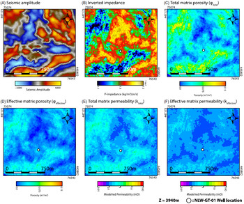
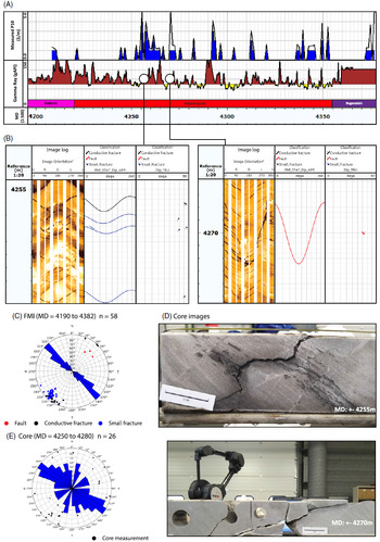


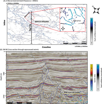


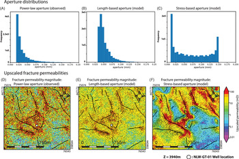


 Open access