


1. INTRODUCTION
During the Weichselian glacial period, large parts of the Arctic were ice covered. At its maximum the Eurasian ice sheet, consisting of both the Barents Sea ice sheet (BSIS) and the Fennoscandian ice sheet (FSIS), merged with the Celtic ice sheet in the south-west and extended all the way up the north continental shelf (Fig. 1), covering both the Barents and the Baltic Seas (Svendsen and others, Reference Svendsen2004a). A close historical equivalent to the West Antarctic ice sheet (WAIS) is the former BSIS. At the Last Glacial Maximum (LGM) the two ice sheets were more or less equivalent in both size and volume but whereas the BSIS completely disappeared, the WAIS endured (Anderson and others, Reference Anderson, Shipp, Lowe, Wellner and Mosola2002; Svendsen and others, Reference Svendsen2004a; Evans and others, Reference Evans, Dowdeswell, Ó Cofaigh, Benham and Anderson2006). Both ice sheets were grounded largely below sea level and both had large, dynamic ice streams that drained them (Andreassen and Winsborrow, Reference Andreassen and Winsborrow2009). The BSIS thus constitutes a close geological analogue to WAIS and its history can provide important insights into the future evolution of the WAIS. Subglacial hydrology is thought to have played a crucial role in the relatively fast disintegration of the BSIS (Winsborrow and others, Reference Winsborrow, Andreassen, Corner and Laberg2010; Bjarnadóttir and others, Reference Bjarnadóttir, Winsborrow and Andreassen2014).

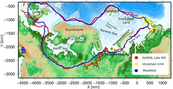
Fig. 1. A map showing the study area as well as the modelled and reconstructed extent of the Eurasian ice sheet at the LGM. The reconstructed extent based on geological evidence from Svendsen and others (Reference Svendsen2004a) is shown in red with uncertain limits in green and modelled extent is shown in blue (for S w = 6).
Temperate ice and subglacial meltwater are typically found either underneath very thick ice due to the geothermal flux and the insulating properties of ice or in areas of high deformation and/or frictional resistance such as closer to the margin (Siegert and others, Reference Siegert, Dowdeswell, Gorman and McIntyre1996). Any subglacial meltwater that forms will drain from areas of high pressure potential towards areas with lower potential. Components of the subglacial drainage network can in general be divided into two different categories or subsystems; (1) an efficient system consisting of fast flowing water in channels carved into ice, bedrock or sediment (Röthlisberger, Reference Röthlisberger1972; Nye and Frank, Reference Nye and Frank1973), exhibiting low water pressures compared with ice overburden or (2) an inefficient system, exhibiting high water pressure, such as sheet flow (thin film) (Weertman, Reference Weertman1966) or flow through connected cavities (Lliboutry, Reference Lliboutry1968) or porous sediment (Shoemaker, Reference Shoemaker1986). Real drainage networks comprise a combination of the two and tend to have both diurnal and seasonal cycles (van de Wal and others, Reference van de Wal2008; Andrews and others, Reference Andrews2014).
Subglacial water lubricates the ice base by effectively separating it from the underlying bed and decreasing the area and force of contact between the two (Iken, Reference Iken1981; Schoof, Reference Schoof2010). Within the sediment column, increasing pore water pressures decrease its yield strength, mainly by separating sediment particles from one another, leading to easier and faster sediment deformation (Tulaczyk and others, Reference Tulaczyk, Kamb and Engelhardt2000). Rapidly moving corridors of ice, ice streams, typically move mostly by either basal slip or by deformation of the underlying sediments, both of which are highly dependent on the availability of subglacial water. In modern-day ice sheets, up to 90% of mass is lost through these fast flowing corridors of ice (Bamber and others, Reference Bamber, Vaughan and Joughin2000). Inclusion of these processes in numerical ice-sheet models is therefore of vast importance for the estimation of future ice loss in polar regions and changes in global sea level. By studying the dynamics of extinct ice sheets and how models respond to perturbations in external forcing we can learn much about how modern ice sheets are likely to respond to a changing climate in the future.
1.1. Previous modelling studies
The Eurasian ice sheet has previously been modelled with 3-D thermomechanically coupled ice-sheet models such as by Payne and Baldwin (Reference Payne and Baldwin1999) who established a connection between past ice streaming and fan-like landform assemblages on a hard-rock area of the Baltic Shield. Although neither accounting for the Barents Sea part of the ice sheet nor subglacial sliding in general, their model output matched reasonably well with available empirical data of the time. Geological and geophysical data from the former Eurasian ice sheet as a whole were later summarized and used for a geological reconstruction of the Quaternary ice sheet development (Svendsen and others, Reference Svendsen2004a, Reference Svendsen, Gataullin, Mangerud and Polyakb). As part of the same program, the Quaternary Environment of the Eurasian North (QUEEN), Siegert and Dowdeswell (Reference Siegert and Dowdeswell2004) used an inverse modelling approach to simulate the Eurasian ice sheets growth and decay, during the late Weichselian, matching the geological evidence presented. They varied climatic inputs in order to optimize the fit between model evolution and empirical data. Another modelling approach was adopted by Forsström and Greve (Reference Forsström and Greve2004) who used the shallow ice approximation (SIA) numerical model, SICOPOLIS (Simulation COde for POLythermal ice sheets), as we do in this study. Their model, although fitting the western limits well, extensively overglaciated the eastern part of the ice sheet, which prompted them to introduce LGM anomalies, or strong west-east gradients in temperature and precipitation forcings, in order to reduce the extent of glaciation in the east, over the Kara Sea and the Pechora lowlands. SICOPOLIS was again used by Clason and others (Reference Clason, Applegate and Holmlund2014) who improved upon previous models by incorporating a parametrization of surface meltwater enhanced sliding (SMES). They produced a model fitting well with empirical data and again confirmed the necessity of strong west-east gradients in both temperature and precipitation to reduce glaciation in the east.
Here, we further build upon the Clason model, introducing a simple representation of the subglacial hydrological system, focussing specifically on the influence of subglacial-water-enhanced sliding on ice dynamics and the temporal evolution of the FSIS and the BSIS, without the inclusion of SMES. In addition, we use the hydrological model to deduce probable locations of past subglacial lakes, their temporal perseverance, size and probability of existence.
2. MODELLING APPROACH
2.1. Ice-sheet model
We use the thermodynamically coupled ice-sheet model SICOPOLIS (Greve, Reference Greve1997) in order to simulate the FSIS and the BSIS. SICOPOLIS is a 3-D, polythermal, two-layer model (temperate and cold ice) that uses a simplified set of equations (SIA) to calculate ice velocities, thickness, age, temperature and water content. Ice is treated as an incompressible fluid where strain rates are related to deviatoric stresses via Glen's flow law (Glen, Reference Glen1955). Ice viscosity depends on temperature, water content and effective strainrate (Duval, Reference Duval1977; Paterson and Budd, Reference Paterson and Budd1982; Duval and Lliboutry, Reference Duval and Lliboutry1985). The SIA is incapable of correctly reproducing ice streams as higher order stresses are neglected although one can mimic their effect through enhanced sliding in temperate regions. Large-scale behaviour of ice sheets is generally well represented however. The model was run, with a horizontal grid size (Δx) of 40 km and a time step (Δt) of 10 a, for 250 ka to allow for sufficient spin-up time and to minimize any errors arising from arbitrarily chosen initial conditions, although we only present results from the last 100 ka with a special focus on the final 30 ka of the Weichselian (40–10 ka) as this is the main study period.
Isostatic adjustment follows the local-lithospere-relaxing-asthenosphere approach where an ice load causes a local displacement of the lithosphere, balanced by a buoyancy force of the viscously deforming asthenosphere (Greve and Blatter, Reference Greve and Blatter2009). Compared with computationally more expensive lithosphere treatments where elasticity is accounted for, the local approach results in a slightly more spatially-concentrated and less smooth isostatic response as there is no lateral effect beyond the ice load of each computational cell (as there is with an elastic lithosphere approach) (Le Meur and Huybrechts, Reference Le Meur and Huybrechts1996). This effect is not too pronounced though and mostly significant in regions with large ice-thickness gradients, such as close to the ice margins (Greve and Blatter, Reference Greve and Blatter2009).
Ice shelves are not treated explicitly, but instead the model is allowed to glaciate the seafloor above a certain threshold depth (1000 m). When ice moves into deeper water, ice thickness is set to zero, which can be considered as a crude form of calving. Sensitivity studies show little dependence on this threshold depth, with the main differences between this and the typically used lower threshold of 500 m being that a small area within the North Sea resists glaciation for the lower threshold (Clason and others, Reference Clason, Applegate and Holmlund2014).
2.2. Climate forcing
We employ the same climatic forcing as in Clason and others (Reference Clason, Applegate and Holmlund2014) where climatic conditions were linked to the NorthGRIP δ 18O ice core record and a synthetic Greenland ice core record based on Antarctic data and the thermal bipolar seesaw model (Andersen and others, Reference Andersen2006; Wolff and others, Reference Wolff, Chappellaz, Blunier, Rasmussen and Svensson2010; Barker and others, Reference Barker2011). Temperatures and precipitation were scaled between present day and LGM conditions using a combination of CFSR (Climate Forecast System Reanalysis) data for present-day conditions (Uppala and others, Reference Uppala2005; Saha and others, Reference Saha2010; Dee and others, Reference Dee2011) and IPSL (Institut Pierre Simon Laplace) CM5A-LR for LGM conditions (Kageyama and others, Reference Kageyama2013). In order to get a realistic ice-sheet extent, comparable with that compiled by Svendsen and others (Reference Svendsen2004a), a linear gradient, from the west to the east, on the LGM temperature data was imposed, reducing temperatures in the west and raising them in the east. For further details see Clason and others (Reference Clason, Applegate and Holmlund2014).
2.3. Subglacial hydrology
Following (Kleiner and Humbert, Reference Kleiner and Humbert2014) we use a subglacial water-flow model where water is assumed to flow in a thin film between the underlying substrate and the ice (Johnson and Fastook, Reference Johnson and Fastook2002; Le Brocq and others, Reference Le Brocq, Payne, Siegert and Alley2009). The time dependent water depth (d) is given by:
 $$\displaystyle{{\partial d} \over {\partial t}} = M - \nabla ({\bi u}_{\rm w} d),$$
where M is the basal melt rate, computed at every time step, and uw is the depth-averaged water velocity. A second equation relating water depth and differences in water pressure to the water velocity can be obtained by assuming that the flow can be described as laminar flow between two parallel plates as (Weertman, Reference Weertman1972):
 $${\bi u}_{\rm w} = \displaystyle{{d^2} \over {12\mu}} \nabla \Phi, $$
where μ is the viscosity of the water and Φ the hydraulic potential. The latter can be written in terms of water pressure p w and an elevation potential
 $$\Phi = \rho _{\rm w} gz_{\rm b} + p_{\rm w}, $$
where ρ w is the density of water, g the gravitational acceleration and z b is the height of the bedrock relative to some fixed datum (WGS84, Polar Stereographic projection).
Water pressure can in turn be described by the ice overburden pressure (H is ice thickness, ρ i is ice density) minus the effective pressure N
 $$p_{\rm w} = \rho _{\rm i} gH - N.$$
Here, we assume that the effective pressure is everywhere equal to zero (Shreve, Reference Shreve1972), which simplifies the pressure potential to a purely geometrical equation where the potential gradient is described as a function of the surface and the bedrock gradient
 $$\nabla \Phi = \rho _{\rm i} g\nabla z_{\rm s} + (\rho _{\rm w} - \rho _{\rm i} )g\nabla z_{\rm b}, $$
where z s represents the elevation of the ice surface.
It is assumed that the timescales governing water flow are much shorter than those governing the flow of ice and that Eqn (1) thus reaches steady state (∂d/∂t = 0) within each time step of the ice flow model. Water fluxes are calculated recursively, at each time step, starting from the top of the hydraulic potential surface, in the direction of the hydraulic gradient following Budd and Warner (Reference Budd and Warner1996). For an overview of different, typically used flux routing numerical schemes see Le Brocq and others (Reference Le Brocq, Payne and Siegert2006).
2.4. Basal sliding
We employ a Weertman-type sliding law that relates the basal shear stress and velocity (Weertman, Reference Weertman1957)
 $${\bi u}_{\rm b} = - C_{\rm b} \vert \tau _{\rm b} \vert ^{\,p - 1} \tau _n^{ - q} {\bi \tau} _{\rm b}, $$
where ub is the basal horizontal velocity, τb the basal shear stress and τ n basal normal pressure, which is taken to be equal to the ice overburden pressure. The sliding law is extended in order to allow for sliding at sub-melt temperatures and the thickness of the water layer following Kleiner and Humbert (Reference Kleiner and Humbert2014) and Johnson and Fastook (Reference Johnson and Fastook2002).
 $$C_{\rm b} = (1 + f_{\rm w} )f_{\rm T} C_{\rm b}^{\rm 0}, $$
 $$f_{\rm w} = (S_{\rm w} - 1)\left[ {1 - {\rm exp}\left( { - \displaystyle{d \over {d_0}}} \right)} \right],$$
where f T = exp(ν(T − T pmp)), ν is the sub-melt sliding parameter, T temperature, T pmp = T 0 − βp the pressure dependent melting point,  $C_{\rm b}^{\rm 0} $ is a basal sliding parameter that depends for example on bed material and roughness, (d 0) is a typical scale of water layer thickness (here equal to 1 mm or 10−3 m) and S w is the maximum increase in sliding velocity due to subglacial water. Here, we test three different values for S w, [1, 3, 6] representing a maximum of a six fold increase in sliding velocity due to the water layer. A two part mask is used for bed roughness ( $C_{\rm b}^{\rm 0} $), a background value of 11.2 m a−1 Pa−1 and 33.6 m a−1 Pa−1 where the bed is considered to consist of a thick deformable layer of soft sediment (Clason and others, Reference Clason, Applegate and Holmlund2014). Numerical values for all other parameters discussed are presented in Table 1.
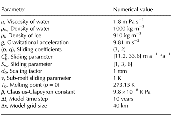
Table 1. Model parameters discussed in the paper

2.5. Subglacial lakes
Model output, such as basal melt rates, temperature, ice thickness and isostatic adjustment are interpolated onto high resolution grids in a post-processing step, for a selection of time slices every 250 years in the period 40–10 ka, and used along with modern day topographic maps of the study area (General Bathymetric Chart of the Oceans (GEBCO), Weatherall and others (Reference Weatherall2015)) for high resolution calculations of meltwater routing (1 km grid size). These can be used to infer possible locations of subglacial lakes and their temporal duration. Before routing is calculated, any local minima (sinks) in the hydraulic potential need to be filled to brink, allowing water to continue further downstream. These local minima represent areas where subglacial water would be likely to pond on its way down the hydraulic potential. By mapping these out we get an idea of potential locations where subglacial lakes might have existed in the past and by looking at a selection of time slices we get a sense of how long they were likely to have persisted throughout changes in the ice-sheet state or configuration. The height to which the sinks need to be adjusted in order to eliminate them is used as a proxy to estimate the potential depth of each subglacial lake, assuming that the change in potential arises solely from a change in water depth (Eqn 3). By summing up the estimated volume of all lakes, we get a rough approximation of total water storage capacity in subglacial lakes for the whole domain. Such a value is unlikely to be of very high accuracy, but relative changes in lake storage capacity with time might be considered to be more reliable. Additionally, although a water-film model is incapable of reproducing channels in a physically meaningful manner, areas where flow of meltwater converges to form a thick water layer can be considered to be likely locations where channels would have formed in the past (Livingstone and others, Reference Livingstone2015).
3. MODEL RESULTS
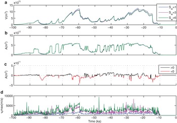
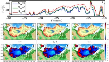
The model results show a two-peaked glacial maximum, with the latter peak occurring ~23.5 ka when both area and volume are at a maximum. We will refer to this peak as the LGM. The ice-sheet extent at the LGM matches well with empirical data (Fig. 1) with relatively small differences in extent between model runs with or without water enhanced sliding (results for S w = 1 are the same as for model run 1 in Clason and others (Reference Clason, Applegate and Holmlund2014)). Maximum thickness of 4125 m is reached slightly later, or at 19 ka for simulations with hydrology-coupled (HC, S w>1) sliding. Maximum horizontal velocities are typically ~3000 m a−1 for S w = 6 with peak values approaching 10 km a−1 over short time periods (Fig. 2c). A stronger coupling (higher S w) between sliding and water layer thickness results in a lower overall ice volume building up with time (Fig. 2a) although the areal extent is not greatly affected (Figs 2b, c). The ice sheet disintegrates rapidly shortly after 15 ka and by 10 ka has completely disappeared.

Fig. 2. Comparison between simulations with different values of the sliding parameter S w for the last 100 ka. Blue in subfigures (a,b,d) represents simulations without HC sliding (S w = 1), purple S w = 3 and green S w = 6. (a) shows total ice volume in m3, (b) shows total area coverage of glacial ice in m2, (c) shows the difference in total area between simulations with (S w = 6) and without (S w = 1) a thin water film. Black denotes points in time when areal coverage is larger for simulations without HC sliding and red otherwise. (d) shows the maximum horizontal velocity of the whole domain at each point in time in  ${\rm m}{\kern 1pt} {\rm a}^{ - {\rm 1}} $.
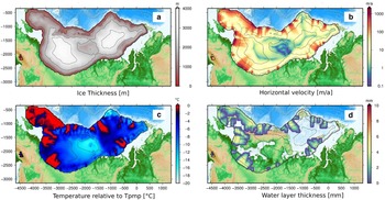
At the LGM, 20% of the ice-sheet base is estimated to be temperate, mostly close to the margin in ice streaming areas. The coldest part of the ice sheet at the LGM, with basal temperatures well below the pressure melting point is roughly over Finland, in the center of the domain (Fig. 3). This is also the thinnest part of the ice sheet at that time and therefore the part where basal temperatures are most influenced by the cold surface temperatures above. There, the ice velocities are close to zero during the LGM and only increase in that area during deglaciation when the ice sheet is smaller and the margin closer.

Fig. 3. (a) Ice sheet thickness in m, (b) horizontal velocity in  ${\rm m}{\kern 1pt} {\rm a}^{ - {\rm 1}} $, (c) basal temperature relative to pressure melting point in °C and (d) water layer thickness in mm for the S w = 6 sliding scenario at 23.5 ka, the point of maximum ice extent and volume.
The model produces two major ice domes that merge ~34 ka with one ice dome centered over the Gulf of Bothnia (FSIS) and the other over the Barents Sea (BSIS, Fig. 3a). The Fennoscandian dome then merges with the Celtic IS shortly before the LGM, or ~26.5 ka to produce one major ice sheet. The eastern extent of the ice sheet, in contrast to many previous modelling attempts, compares well with geological reconstructions (Fig. 1).
Incorporation of HC sliding improves the models ability to mimic ice streams and spatially confine their location. SIA generally produces broad areas of fast flow whereas the inclusion of hydrology-coupled sliding limits and confines fast-flowing areas to temperate areas with a thick water layer (Fig. 4) and thus better mimics real velocity patterns. Faster sliding leads to a reduction in the temperate area fraction (TAF) of basal ice, however, the width of ice streaming areas is probably still somewhat overestimated because of the limited grid resolution of the numerical model and simplified model physics.

Fig. 4. (a) TAF of the Eurasian ice sheet between 40 and 10 ka. (b,c,d) a comparison of horizontal velocity in  ${\rm m}{\kern 1pt} {\rm a}^{ - {\rm 1}} $ and temperature (e,f,g) in C relative to pressure melting point for the three sliding scenarios considered (at 20 ka). (b,e) are with S w = 6, (c,f) with S w = 3 and (d,g) without HC sliding (S w = 1).
Water is routed along the direction of the largest gradient according to Eqn (5) (Budd and Warner, Reference Budd and Warner1996) and is limited to temperate areas of the ice sheet. The calculated thickness of the water layer used in the model rarely exceeds 6 mm (Fig. 3d), consistent with the thin-film assumption. No extra bedrock smoothing is applied before meltwater is routed along the base to the margin as the 40 km grid resolution already represents considerable averaging simply because of the large grid size.
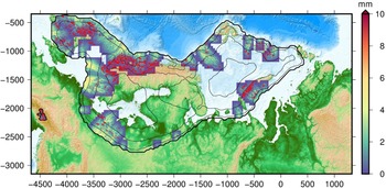
An example of water layer thickness at 23.5 ka, using interpolated model results and modified high-resolution bathymetry (1 km grid size) is presented in Figure 5. Semicircular areas in red depict sinks in the hydraulic potential where water would likely pond on its way towards the margin and routing of subglacial water is limited to areas of the ice sheet with a temperate base.

Fig. 5. Map of water layer thickness at 23.5 ka calculated with a 1 km resolution bathymetric grid. Sinks in the hydraulic potential (potential subglacial lakes) are marked with red (S w = 6).
Several subglacial lakes are predicted to have existed during the last glacial cycle (Fig. 6). Particularly in the Norwegian fjords and valleys as well as on the western side of Novaya Zemlya although the bathymetry data on either side of Novaya Zemlya is not of high quality. The island itself represents a significant hydrological barrier to subglacial flow of water with ice flowing generally from the west to the east, over the island and large parts of the area having a temperate base during much of the glaciation (Fig. 5). Few lakes probably existed in the Barents Sea area and on Svalbard compared with the Scandinavian mainland.

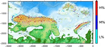
Fig. 6. Map showing all predicted lake locations during the period 40–10 ka, color-coded based on perceived probability of existence. A deep, temporally persistent lake is deemed as having a higher probability of having existed than a shallow, shortlived one. Calculated with S w = 6.
A criterion for the likelihood of a subglacial lake having existed is taken as the product of the estimated lake depth for each time slice and the time each cell persists as part of a subglacial lake. This is done with a grid resolution of 1 km both with and without smoothing (5 km) of the underlying bathymetry. Smoothing eliminates mostly small, shallow sinks of the hydrological potential that would otherwise show up as potential lakes. For completeness and in order to separate these small shallow areas from the deeper and larger potential lake locations, the routing is calculated without smoothing as well. These shallow areas are represented by a yellow color in Figure 6. All grid cells are then ranked with the above criteria, normalized and given a score (H)igh, (M)edium or (L)ow based on the probability of each cell having been part of a subglacial lake, with H representing lakes that are both deep and temporally stable and can thus be considered to be more likely candidates. Each category contains one third of all cells marked as having pertained to a subglacial lake at some point.
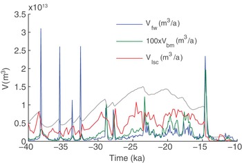
Figure 7 shows the temporal evolution of total lake storage capacity (LSC) as a function of time for the time period 40–10 ka. Changes in ice-sheet geometry, switches in the thermal regime or deflections of the lithosphere all affect the storage capacity of subglacial water. Here we have opted for the more conservative estimate of lake storage, assuming that any change necessary in the hydraulic potential needed to fill local minima would come from a change in water level alone, leaving ice thickness untouched. This leads to a total amount of stored water of the same order of magnitude as estimated for Antarctica (Pattyn, Reference Pattyn2008). The LSC generally follows the ice-sheet evolution with sharp drops in volume and peaks in freshwater production associated with drops in LSC as well. The rate of loss in storage capacity of subglacial water can equal or surpass the amount of basal water produced during the same time, indicating that a considerable amount of subglacial water is poured out during deglacial periods. A larger more extensive ice sheet tends to support a greater storage of subglacial water underneath the ice sheet.

Fig. 7. Total freshwater production (V fw), basal melt volume (100 × V bm) and lake storage capacity (V lsc) in m3 a−1 from 40 to 10 ka (S w = 6). Ice volume is shown in gray in the background for comparison (not to scale).
4. DISCUSSION
Overall, the modelled LGM extent of the FSIS and the BSIS matches well with the geological reconstructions of the former ice sheets (Svendsen and others, Reference Svendsen2004a, Reference Svendsen, Gataullin, Mangerud and Polyakb), with the inclusion of subglacial hydrology representing a slight improvement both in extent and volume in the Barents Sea region. We have used the same climate forcings as Clason and others (Reference Clason, Applegate and Holmlund2014), which along with older work of Siegert and Dowdeswell (Reference Siegert and Dowdeswell2004) and Forsström and Greve (Reference Forsström and Greve2004) confirmed the need for strong west-east gradients in both temperature and precipitation patterns.
4.1. Hydrology
The meltwater-enhanced sliding has a strong effect on the evolution of the ice sheets. Sliding velocities are coupled to the evolution of the thin water film and increase with increasing film thickness. This leads to considerably lower ice thickness and volume building up over time. During the early stages of inception little to no differences are seen in either volume or extent as the ice sheet is mostly cold-based. As soon as a part of the margin reaches pressure melting point and sliding picks up, it draws down ice from the surrounding area, deflecting flow directions towards the lowered surface. The total ice-sheet extent is not greatly affected by HC sliding. Most notable are the differences during or following a warm period and a sharp decrease in volume where the lower thickness of the HC ice sheet means that it is more vulnerable to the higher temperatures at lower altitudes and thus experiences more surface melt and a faster decline. During ice-sheet growth and at peaks in volume the areal extent is generally slightly larger.
The effect of HC sliding on the basal temperatures, and most notably the percentage of the bed that is actually at pressure melting is greater. As can be seen from Figure 4, a much larger part of the bed is at pressure melting for simulations without HC ice dynamics. When the movement of ice changes from flow by internal deformation to flow by rapid basal sliding, this affects the heat balance of the ice. When basal sliding ensues, heat generated by internal deformation within the ice column decreases but gets somewhat compensated for by frictional heating between the sliding ice and the underlying substrate. This however does not explain why models disregarding subglacial hydrology and its effect on sliding would overestimate temperate areas of the ice sheet. The explanation lies in the fact that for the HC sliding scenario, faster sliding leads to increased advection of cold ice from above in the transition zone, in addition to less deformational energy being available due to the lower ice thickness. Models neglecting subglacial hydrology are thus likely to overestimate temperate areas of the base as well as total ice volume compared with models that include subglacial hydrology and any associated enhancement in sliding. In simple models, such as the SIA, all stresses except vertical shearing are neglected whereas in reality, in ice streaming areas, deformation of ice is mostly due to longitudinal and lateral stresses and the internal deformational energy therefore incorrectly estimated. The SIA is technically invalid in such areas and along ice-sheet margins and ice divides in general (Baral and others, Reference Baral, Hutter and Greve2001). As the ratio between movement by sliding versus movement by internal deformation increases, the less accurate the SIA becomes (Gudmundsson, Reference Gudmundsson2003). Including HC sliding in such models, although physically still lacking, is nevertheless worthwhile as it entails a better representation of reality and delineation of ice-streaming areas.
4.2. Subglacial lakes
Many subglacial lakes are predicted to have existed during the last glacial cycle (Fig. 6) and several of them seem to have persisted over thousands of years and reached considerable depths. Not many lakes seem to form in the Barents Sea itself, an area of active palaeo-hydrology research, as the bathymetry there is generally quite flat and smooth. The most likely locations for formation of subglacial lakes in the BS seem to be around Spitsbergenbanken and Central Barents Sea (Fig. 1). Many lakes forming there would likely have been ‘active’ lakes with low water depths, short residence times and fast circulation of water much like lakes in similar settings in West Antarctica (Gray and others, Reference Gray2005; Fricker and others, Reference Fricker, Scambos, Bindschadler and Padman2007). Drainage could be frequent and possibly complete on decadal timescales or slower, in which case the lake roof would come in and out of contact with the underlying sediments, thus complicating the possibility of identifying them today from geological remains. These predictions however, should be taken with precaution as several of the locations could be related to geomorphological features on the seafloor, features related to the deglaciation of the area, which would not have been present in its modern-day form during the time when a subglacial lake is predicted to have formed there.
Subglacial lakes represent areas of the ice-sheet base, fixed at the pressure melting point and incapable of exerting any shear stress on the overlying ice. The ice therefore slides freely above it, being held back only by longitudinal and lateral stresses. As all stress components are generally important around subglacial lakes, the SIA approximation is unable to account for them in a satisfactory way. Ice generally moves more like an ice shelf over large lakes, with uniform velocity. Deformational and frictional heating thus largely disappear in the ice above them (Gudlaugsson and others, Reference Gudlaugsson, Humbert, Kleiner, Kohler and Andreassen2016). As the ice speeds up it gets drawn down by vertical flow at the edges and the ice surface tends to level above it. This effect that subglacial lakes have on the ice surface also affects the hydrological potential and it has been hypothesized that this surface levelling has a stabilizing effect on their presence through deglaciation cycles or changes in ice configuration (Livingstone and others, Reference Livingstone2012). They are thus likely to persist once formed, and lakes can be found in places, after reorganization of the ice-sheet geometry, where no corresponding sink in the hydrological potential, based on coarse geometry data alone, can be estimated.
4.3. Water storage
Subglacial lakes accumulate and store considerable amounts of meltwater and some estimates put the amount of stored subglacial water in Antarctica at ~12 000–24 000 km3, equivalent to ~0.5–1 m thick water layer if spread out evenly underneath the entire Antarctic ice sheet (Pattyn, Reference Pattyn2008). Typical basal meltrates are on the order of a few millimetres per year and the time it takes for the ice sheet to produce the amount of stored water is thus on the order of a few hundred to a thousand years. During the last 100 ka of its existence, the Eurasian IS went through several phases of deglaciation followed by repeated regrowth until its final demise ~10 ka ago. Deglaciation typically occurs rapidly in comparison with growth and as we see in its final stages, the ice sheet almost completely disappeared over a period of roughly a thousand years from 13 to 12 ka (Fig. 2). Such drastic changes in ice-sheet geometry and state have profound influences on the subglacial hydrological system. Not only do basal melt rates peak during deglaciation phases, but there are also profound changes in the storage of subglacial water due to the reconfiguration of the ice-sheet geometry and isostatic uplift. The amount of water draining from subglacial lakes can therefore drastically increase the output of subglacial water reaching the margin during deglaciation. The effect that this will have on ice-sheet dynamics in general will depend on how the water is transported downstream, either in a channelized system or via a distributed system. Its effects would range from little to a potentially significant increase in average ice velocities as witnessed at Byrd Glacier in East Antarctica a decade ago (Stearns and others, Reference Stearns, Smith and Hamilton2008) with faster deglaciation pursuing.
5. CONCLUSIONS
Water enhanced sliding leads to both a drop in ice volume and thickness and due to increased advection of cold ice from above and less available deformational energy, the fraction of the bed at pressure melting is reduced. Several subglacial lakes are predicted to have existed underneath the FSIS and the BSIS, some of which coincide with large surface lakes in Scandinavia at present. A considerable amount of water will have been stored in these lakes during glacial times and flushed out during deglaciation phases, potentially multiplying the amount of available subglacial water in motion. A simple thin-film water model is unable to capture the true nature of such an increase, as channel formation is excluded and all added water leads to faster sliding. The question remains, what effect such dynamic water storage in both lakes and sediment would have on ice dynamics in general and future modelling efforts will have to focus on not only more realistic models of ice and water flow but also on including dynamic storage of subglacial water.
ACKNOWLEDGEMENTS
Funding for this work came from the Research School in Arctic Marine Geology and Geophysics (AMGG) at the University of Tromsø and from the Research Council of Norway (RCN), Statoil, Det Norske ASA and BG group Norway (grant 200672) to the PetroMaks project ‘Glaciations in the Barents Sea area (GlaciBar)’, This is also a contribution to the Centre of Excellence: Arctic Gas Hydrate, Environment and Climate (CAGE) funded by RCN (grant 223259). We thank two anonymous reviewers and the scientific editors for reviews and comments that helped improve this paper.

 Open access