

1. INTRODUCTION
The past decade has seen major advances in GNSS technology. However, in dense urban areas, known as ‘urban canyons’, the poor performance of GNSS positioning has remained a major problem in navigation. This is mainly because tall buildings block, reflect and diffract signals in urban canyons. As a result, in some locations, there are insufficient signals for a navigation solution; while in other locations, a solution can only be formed if Non-Line-Of-Sight (NLOS) signals, which exhibit significant positive biases, are used. Ranging errors due to NLOS signal propagation are often categorised as multipath errors. However, this is misleading as the errors can often be much larger and different mitigation techniques are generally required (Ercek et al., Reference Ercek, De Doncker, Grenez and Navstar2006; Walker and Kubik, Reference Walker and Kubik1996).
Increasing the number of Global Navigation Satellite Systems (GNSS) signals by using GLObal NAvigation Satellite System (GLONASS), Galileo and Compass can significantly improve the availability of direct Line-Of-Sight (LOS) signals. The principal aim of this paper is to quantify this improvement in urban environments.
Until recently, accurate prediction of satellite availability in cities has been difficult due to the complex environment. However, 3-Dimensional (3-D) city models, or 3-D Geographic Information Systems (GIS) are becoming more accurate and more widely available, providing the capability to predict LOS availability accurately. A comparison of simulations and real observations has been conducted for GPS/GLONASS/Galileo satellites using 3-D spatial information (Kim et al., Reference Kim, Park and Lee2009). The LOS performance of GPS/GLONASS/Galileo in urban environments was evaluated by simulating a route in an urban environment (Ji et al., Reference Ji, Chen, Ding, Chen, Zhao and Hu2010).
Besides LOS availability, 3-D simulations have also been used to investigate multipath, diffracted and reflected signals. A detailed GNSS availability prediction considering LOS, diffracted and re-radiated signals has been tested using a 3-D city model (Bradbury, Reference Bradbury2007; Bradbury et al., Reference Bradbury, Ziebart, Cross, Boulton and Read2007). A 3-D GIS model has been used in GPS multipath and LOS prediction and accuracy evaluation (Suh and Shibasaki, Reference Suh and Shibasaki2007).
However, pedestrian and vehicle GNSS navigation users suffer signal degradation with different characteristics, which has not been investigated. Moreover, to the authors' knowledge, little research has considered the effect of the emerging Chinese ‘Compass’ system on the overall GNSS navigation performance in urban canyons.
In this work, a model has been developed to predict GNSS performance in urban areas using a 3-D architectural city model. Section 2 gives a brief introduction to the city model and describes the satellite visibility determination process. Section 3 compares selected results from the simulation with real-world observations to validate the simulation and investigates the effects of including diffracted signal in the model. Section 4 then describes the simulation scenarios for predicting future GNSS performance in urban areas and presents the results. Two sets of simulations representing pedestrian and vehicle routes in central London were selected to evaluate performance using different combinations of GNSS constellations. The results are analysed to determine the average number of satellites directly visible at each test point and the availability of 4-satellite, 5-satellite and good geometry solutions. Along-street and cross-street accuracy are also compared. Finally, the conclusions are summarised and their implications for the design of future urban navigation systems are discussed.
2. SATELLITE VISIBILITY DETERMINATION
Determining satellite visibility requires building, satellite and user route data, expressed in a common reference frame, together with a computationally efficient algorithm for testing. This section describes how this is achieved.
2.1. City Models
The software toolkit developed for this study stores and processes 3-D city model data using Virtual Reality Modelling Language (VRML), an international standard format. Model data in other formats can be transformed to VRML. Buildings in VRML format are represented by structures, which in turn compromise polygons (normally triangle meshes).
Throughout this work, a real 3-D city model of part of central London (around Aldgate) supplied by ZMapping Ltd has been used. The model has a high level of detail and decimetre-level accuracy.
2.2. Data Preparation
Data sets for simulation consist of GNSS satellite orbits, building geometries from the 3-D city model and user routes. Four GNSS systems, comprising GPS, GLONASS, Galileo and Compass, have been deployed in the simulation. The GPS and GLONASS satellite positions are computed from the satellite broadcast ephemeris data published online by the International GNSS Service (IGS). Galileo orbits are synthesized using the description in the Space Interface Control Document (GJU, 2006). The Compass orbits are generated from an unofficial description of the full global system (Van Diggelen, Reference Van Diggelen2009).
Building geometries are abstracted from the city model VRML file. User routes are generated from the city model using Rhinoceros, a 3-D modelling tool.
It is imperative to express all geometric information in a common coordinate frame. Thus, coordinates of the satellites, user positions and model data, are transformed into an Earth-Centred, Earth-Fixed (ECEF) frame based on the World Geodetic System 1984 (WGS-84) datum. Satellite orbit data for GLONASS have been transformed from the Parametrop Zemp 1990 (PZ90.02) datum into WGS-84. The Grid InQuest 6.0 DLL (Quest Geo Solutions Ltd, 2004) was used to transform the 3-D city model data from the Ordnance Survey of Great Britain 1936 (OSGB-36) datum, used in the UK and Ireland, to the International Terrestrial Reference Frame (ITRF) 2005 datum, which is within centimetres of WGS-84.
2.3. Visibility Determination Algorithm
Satellite visibility for a user-satellite LOS with respect to one building triangle can be determined using the line and triangle intersection determination algorithm described in Appendix A. In a simple satellite visibility determination algorithm, each detailed building structure (comprising about 100,000 surfaces) within the 3-D city model is tested for blockage of the user-satellite LOS. Moreover, each of these tests is applied to every satellite above the elevation mask angle in up to four GNSS constellations. This basic approach consumes far too much processing power for either real-time implementation or a large batch of simulations. Therefore, in the satellite visibility determination algorithm used for this study, three changes have been made to significantly improve the efficiency.
• Optimization 1. Building data that is beyond 300 m is excluded because buildings 300 m away will only block satellite signals at low elevation angles that are normally below the receiver's masking angle. Even a building as high as 50 m, 300 m away cannot block satellites at elevations greater than 10°.
• Optimization 2. When considering multiple user locations, buildings that have been found to block the user-satellite vector at one location are tested first at the next location. This is an example of the priority queue principle.
• Optimization 3. Instead of using the city model to compute the visibility of each satellite directly, it is useful to determine the boundary of the buildings from the user's perspective. A sky plot of the building boundary in terms of elevation and azimuth is thus obtained. Then, satellite visibility is easily determined by comparing the satellite's elevation with the building boundary's elevation, at the same azimuth. This approach is more efficient where a great number of satellite visibility tests are performed at the same location. For real-time visibility determination, building boundaries may be pre-computed over a grid of possible user locations and stored.
The building boundary is determined at a number of different azimuths, spaced at regular intervals and spanning 360°. For each azimuth, the building boundary is the highest elevation at which the LOS from a virtual satellite at that azimuth is blocked. This is determined using bisection; firstly the visibility of a virtual satellite at a 45° elevation is tested. If it is blocked, then the higher elevation region is refined in bisection and the next test is performed at an elevation of 45°+45°/2=67·5° of elevation; otherwise, the satellite is visible and the lower elevation region is refined, so the next test is at 45°−45°/2=22·5° of elevation. The bisection process continues until the boundary has been determined to within a 1° elevation resolution. As a result, seven satellite visibility tests must be performed at each azimuth.
With a 1° azimuth resolution, which is relatively high, 7*360=2520 satellite visibility tests are required to determine the building boundary at each user location, which still imposes a considerable computational load. Therefore, lower azimuth resolutions were considered. Figure 1 compares the building boundaries obtained with 2°, 10°, and 30° azimuth resolutions. A compromise azimuth interval of 10° may be used in real-time implementations. This approach is more efficient than the basic approach, requiring 7 * (360°/10°)=252 satellite visibility tests to be performed at each location. The building boundaries can then be used for any satellite visibility prediction at the same location at any epoch. There is a trade-off between computation load and satellite prediction accuracy.
Sky plot of building boundaries from the perspective of GNSS users with different azimuth resolutions. (The blue lines represent the roof and edge boundary of the buildings surrounding the user; the light blue area represents the visible sky).

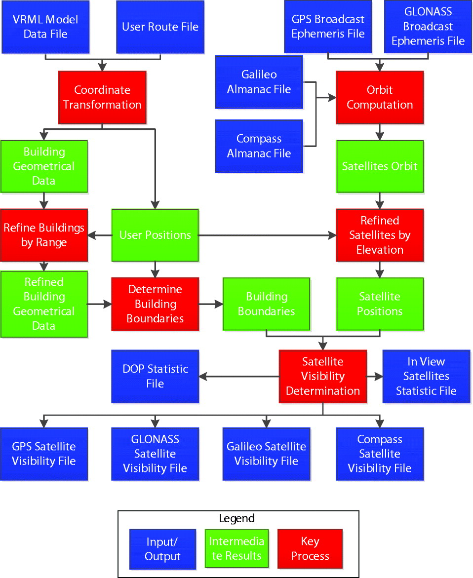
The software toolkit for all data pre-processing and the satellite visibility determination was developed in C++. Figure 2 shows the software flowchart.
Software flowchart for satellite visibility determination.
3. EXPERIMENTAL VERIFICATION
3.1. Experimental Results
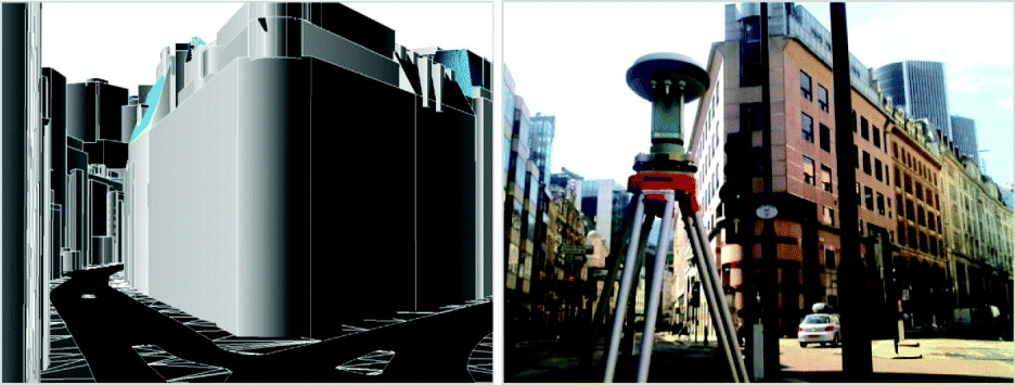
Experiments have been carried out to compare the model-predicted satellite visibility with real-world observations. Two two-hour GNSS data collection sessions were conducted in different urban environments (named test points 1 and 2). Views of the real urban environment and the city model at test point 2 are shown in Figure 3.
View from test point 2: the 3-D city model (left) and the real environment (right).
Accurate positions of the test sites were determined by differential carrier phase GNSS using four Ordnance Survey reference stations within 50 km.
A comparison is made between observed and predicted satellite visibility every 30 seconds. Figure 4 and Figure 5 present the comparisons between real and predicted satellite visibility for test points 1 and 2, respectively. The building boundary for prediction was determined using a 1° azimuth interval. In these two figures, G denotes GPS satellites and R refers to GLONASS satellites.
Comparison of observed and predicted GPS and GLONASS satellite visibility at test point 1.

Comparison of observed and predicted GPS and GLONASS satellite visibility at test point 2.

The results show that in most cases, the predicted satellite visibility agrees with the experimental observation (blue and grey dots in Figure 4 and Figure 5). However, there are a significant number of cases where they disagree (shown as green and red dots). Reasons for predicting a signal that is not observed include new buildings that are not in the database, trees and street furniture; all of these were observed at the test sites. Obstruction of a signal by a small object can account for many of the relatively short interruptions to signal tracking seen in the test data.
Reasons for observing a signal when none is predicted include diffraction, reception of reflected signals via NLOS paths, city model precision limitations and buildings appearing in the city model that were subsequently demolished. For the purposes of predicting GNSS availability and precision across an example urban environment, the effects of demolition and construction of buildings may be assumed to cancel. Furthermore, NLOS signals may be neglected as they exhibit large range biases so should be filtered out of the position solution where possible. However, diffracted signals exhibit relatively small biases, so may be considered useful for positioning. The intermittent reception observed for many of the unpredicted signals is characteristic of diffraction (Bradbury, Reference Bradbury2007). Therefore, this was investigated further.
3.2. Diffraction Modelling
Diffraction occurs at the edge of a building (or other obstacle) when the incoming signal is partially blocked, noting that the path taken by a GNSS signal is several decimetres wide. There are two approaches to predicting the effect of diffraction on satellite visibility using a 3-D city model. The first one would be to numerically determine the diffraction field based on every physical factor, including the surface of building, the angle of incidence of the signal and the properties of the GNSS user equipment. This method is impractical because the necessary information about the building materials and antenna characteristics is difficult to obtain and the computational complexity is high. The second, much simpler, approach has been adopted here. This simply extends the building boundary used for satellite visibility determination by adding a diffraction region to model the diffraction effect around building's edge. Thus, wherever the LOS intersects the diffraction region, the signal is classified as potentially diffracted instead of blocked (Walker and Kubik, Reference Walker and Kubik1996; Bradbury, Reference Bradbury2007). Both horizontal and vertical edges are considered for diffraction modelling. Here, a 3°-wide diffraction region was modelled.
Figure 6 and 7 show that using the implemented diffraction model, the satellite visibility prediction is closer to the real observations. However, this diffraction model can only predict strong diffraction, when the signal to noise ratio decreases by no more than 10 dB-Hz from its normal value. Weaker signals are less useful for navigation. Figure 7 also shows that the signal characteristics in an urban area can sometimes be very complex. Nevertheless, the model still successfully predicted the strongest signals.
Comparison between measured signal to noise ratio (SNR) and GNSS signal availability for GPS PRN 10 at test point 2 (Diffraction considered).

Comparison between measured signal to noise ratio (SNR) and GNSS signal availability for GLONASS 7 at test point 1 (Diffraction considered).

Figures 8 and 9 show that the diffraction model works reasonably well for most other satellites in the experiments, increasing the reliability of the satellite visibility prediction.
Comparison of observed and predicted GPS and GLONASS satellite visibility at test point 1 with diffraction model.

Comparison of observed and predicted GPS and GLONASS satellite visibility at test point 1 with diffraction model.

4. SIMULATION PERFORMANCE ANALYSIS
This section describes the simulations conducted to predict multi-constellation GNSS performance in urban canyons. Section 4.1 describes the design of simulation. The results are then presented and analysed in Sections 4.2 and 4.3, focusing on direct LOS signal availability and Dilution Of Precision (DOP), respectively.
4.1. Design of Simulation
Two routes, representing vehicle and pedestrian motion, were generated to evaluate GNSS navigation performance by simulation in urban environments. Both routes pass through the same environment with the pedestrian route closer to the building, as shown in Figure 10.
Routes representing vehicle and pedestrian motion (perspective view in the left; top view in the right).

There are four important requirements of any navigation system: accuracy, availability, continuity and integrity (Misra and Enge, Reference Misra and Enge2010; Groves, Reference Groves2008). Thus, for both routes, there are three performance criteria that can be evaluated using the 3-D city model: availability, integrity and precision were evaluated. Comparisons were then made between different scenarios with various satellite constellations in operation.
The particular area from the London city model chosen for the simulations is around Lloyd's of London and Aldgate where there are tall buildings, as shown in Figure 10.
4.2. Performance Evaluation Based on Satellite Numbers in View
Figure 11 shows the average number of satellites in view across all epochs at each user location including useful diffracted signals. To enable contributions of different GNSS constellations to be compared, the four colour bars represent the additional average number of satellites for each successive scenario. Thus, the total is obtained by summing the appropriate number of colour bars. As shown in Figure 10, user locations with even point IDs are between junctions and those with odd point IDs are at junctions.
Daily average number of satellites in view for the pedestrian route (top) and the vehicle route (bottom).
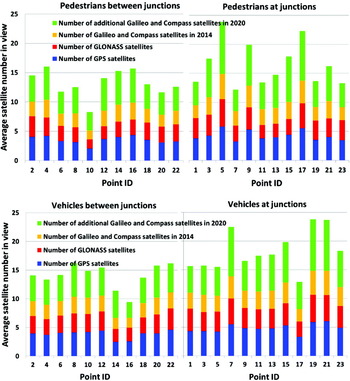
As expected, the histograms in Figure 11 indicate that with more satellite constellations operational, more satellites will be in view in city canyons. With only GPS used, the average number of visible satellites is less than four at many locations, which is not sufficient to provide a positioning solution. Even the combination of GPS and GLONASS fails to provide an average of more than five visible satellites at a few locations. However, with the addition of Galileo and Compass, the average visibility including diffracted signals is at least eight satellites, except at pedestrian Point 10, which is close to a tall building. These results illustrate the poor GNSS performance that can arise in challenging urban environments due to buildings blocking the satellite signals and show the potential benefit of the new GNSS constellations.
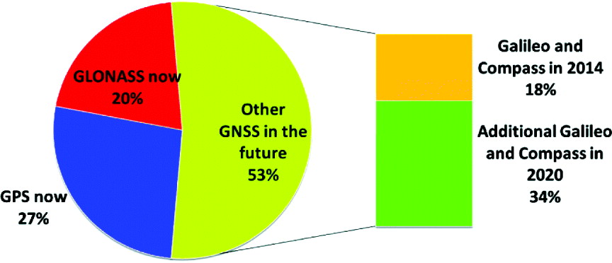
Figure 12 shows how the different constellations contribute to GNSS availability averaged across all the urban environments considered. It is apparent from the chart that GNSS signal availability will increase significantly if all of the additional satellites proposed for launch by 2020 become operational.
Average contribution of each constellation to the number of satellites in view for the 2020 scenario across all pedestrian and vehicle locations.
To compare the performance of individual GNSS constellations now and in the future, a simple statistical analysis was conducted based on data from both pedestrian and vehicle routes. Figure 13 shows the relationship between the type of user location and GNSS signal availability for each GNSS constellation scenario. As expected, there is a clear trend that the number of satellites in view increases with the number of satellites in operation. Interestingly, the figure also shows consistently fewer satellites in view for the pedestrian scenarios compared with the vehicle scenarios, as well as fewer satellites in view for locations between junctions than locations at junctions. The difference may be caused by the pedestrian route being close to the buildings, resulting in more signals being blocked by surrounding buildings. Similarly, the locations between junctions are typically surrounded by more buildings than the locations at junctions.
Average satellite numbers with respect to different type of user locations.

As GNSS user equipment normally needs at least four satellites to provide a navigation solution, GNSS availability is assessed by determining the percentage of time for points on each route when at least four satellites are directly in view with each combination of GNSS constellations. Furthermore, to evaluate the integrity of GNSS in an urban environment, the percentage of time when at least five satellites are directly in view has also been determined. This is because at least five satellites are required for Receiver Autonomous Integrity Monitoring (RAIM).
For both the pedestrian and the vehicle routes, Figure 14 compares the percentage of time over a day when GNSS is available for a positioning solution and for RAIM under each simulation scenario. The average availability across all locations in each category is shown along with the percentage of time at which each criterion is met simultaneously at all locations within that category. The simultaneous availability data provides an indication of the continuity performance.
Percentage of time when the number of satellites is enough for positioning (4 or more satellites) and for RAIM processing (5 or more satellites).
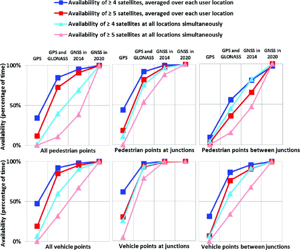
It can be seen from the charts that the availability of both a position solution and RAIM is notably better for a vehicle-based user than for a pedestrian user. However, even for the vehicle route, all four GNSS constellations are required for close to 100% positioning availability and high RAIM availability. Performance is unreliable even for the GNSS in 2014 scenario. Performance along the pedestrian route is normally poorer, particularly at points between junctions. Therefore, even with four fully-deployed constellations, robust and reliable pedestrian positioning in challenging urban environments cannot be achieved using conventional GNSS positioning alone.
4.3. Performance Evaluation Based on Dilution of Precision
For this study, only the horizontal performance is studied as this is the main concern of GNSS users in urban canyons. The DOPs investigated in this paper are the Horizontal DOP (HDOP), the Along-street DOP (ADOP) and the Cross-street DOP (CDOP). ‘Along-street’ is the direction along the street which the user is on; ‘Cross-street’ is the perpendicular direction across the street. In an urban canyon, most satellite LOS will be much closer to the ‘Along-street’ direction than the ‘Cross-street’ direction.
The HDOP, ADOP and CDOP solutions are each considered acceptable when the corresponding DOP is below 5·0. For each simulation scenario, Figure 15 shows the average percentage of time when criteria are met over each user location and the percentage of time the criteria are met at all locations simultaneously. DOP is calculated as described in (Misra and Enge, Reference Misra and Enge2010, Groves, Reference Groves2008).
Percentage of time when the HDOP, along street DOP and cross street DOP are below 5, for each scenario.

Figure 15 shows that, on average, the ADOP is smaller than the CDOP as would be expected from the geometry of the unblocked signals. This is more significant for the pedestrian route. For the locations between junctions the overall precision is poorer than at the junctions. For all of the simulation scenarios, the DOP criteria are met more often along the vehicle route than the pedestrian route. This is consistent with the availability results presented in the previous section. Even with all four constellations, the HDOP criterion is met across the whole route simultaneously only 69·1% of the time for the pedestrian route and 90·4% of the time for the vehicle route.
5. CONCLUSIONS AND DISCUSSION
An optimized satellite visibility determination algorithm has been developed for predicting GNSS performance in urban environments using 3-D building models.
The simulation was verified at two test points with field trials, which demonstrated that direct Line Of Sight (LOS) signals can be predicted using the model. However, due to the complexity of the environment, diffracted and reflected signals were also observed that the original model did not predict. As diffracted signals are potentially useful in positioning, the simulation has been modified to predict them. Verification with real observation shows the implemented diffraction model successfully predicted most of the strong diffracted signals.
Positioning performance using different combinations of Global Navigation Satellite Systems (GNSS), including Global Positing System (GPS), GLObal NAvigation Satellite System (GLONASS), Galileo and Compass has been evaluated by simulation using a 3-D model of London. Solution availability, Receiver Autonomous Integrity Monitoring (RAIM) availability and precision have been assessed for both pedestrian and vehicle routes within a urban environments.
Positioning performance using GPS and GLONASS was found to be unreliable at some of the locations evaluated. Performance using all four GNSS constellations was predicted to be much better, but still unreliable at a few of the locations. Performance was better along the vehicle route than the pedestrian route, which is closer to the buildings; and was better at junctions than between them, where there are typically more buildings. Finally, positioning precision was found to be generally poorer in the ‘Cross-street’ direction than in the ‘Along-street’ direction, because the buildings constrain the satellite signal geometry.
GNSS signal availability has been quantitatively verified to double in year 2020. However, even with four constellations, GNSS performance will still be unreliable at some urban locations in 2020.
Thus, to ensure a reliable positioning service in urban canyons, traditional GNSS should be augmented with other techniques. There are a number of methods, including combining GNSS with other signals, sensors and data sources in an integrated navigation system (Groves, Reference Groves2008; Farrell, Reference Farrell2008). Another solution is GNSS shadow matching, which can potentially improve the across-street positioning accuracy by comparing the observed GNSS signal availability with that predicted using a 3-D city model (Groves, Reference Groves2011; Wang et al., Reference Wang, Groves and Ziebart2011; Groves et al., Reference Groves, Wang and Ziebart2012).
For many applications, the modelling technique presented in this paper could be used to predict the best route through a city at a given time, or the best time to perform GNSS positioning at a given location. This technique could also be applied to GNSS signal prediction in mountainous area by using a digital elevation model (DEM) instead of a city model.
ACKNOWLEDGEMENTS
The authors would like to thank Dr. Joe Bradbury for his help on 3-D model processing; Christopher Atkins, Santosh Bhattarai and Dr. Ziyi Jiang, for their help on experiments; Dr. Mojtaba Bahrami and Peter Stacey for their advice on GNSS algorithm development; and Dr. Xingwang Yu for his support on Compass and Galileo orbit computation. This work has been jointly funded by the UCL Engineering Faculty Scholarship Scheme and the Chinese Scholarship Council.
APPENDIX A
LINE AND TRIANGLE INTERSECTION DETERMINATION ALGORITHM
Algorithms testing direct Line-Of-Sight (LOS) visibility are mature in computer vision and are known as line segment-plane collision detection. Among those algorithms, one suitable for use in determining whether a satellite is blocked by buildings is described in this Appendix.
A.1. GEOMETRICAL REPRESENTATION IN SATELLITE VISIBILITY DETERMINATION
The satellite position and user position are denoted S and U in the model, respectively. The buildings in the city model are each represented by multiple triangles (triangle meshes). Consider a triangle ΔABC with vertices A, B and C. The intersection point of the segment US (LOS vector) and the plane containing ΔABC is denoted I. The vector rAB denote the position of point B with respect to point A defining the line ![]() . All other vectors are similarly defined. The normal vector to ΔABC is n. The origin is O. This is illustrated in Figure A1.
. All other vectors are similarly defined. The normal vector to ΔABC is n. The origin is O. This is illustrated in Figure A1.
Intersection between user-satellite line of sight and a triangular component of a building model.

A.2. INTERSECTION ALGORITHM
Ray and triangle intersection is a common operation in computer graphics. A three-step method is implemented comprising the following steps.
• Step 1. Determine whether there is an intersection of the plane containing ΔABC and the segment US.
• Step 2. Compute the point of intersection I where it exists.
• Step 3. Test whether the point of intersection I is inside or outside the boundary of ΔABC.
The steps are now described in more detail. Equations (A1) and (A2) show vectors in the plain of ΔABC.
The normal vector to ΔABC:
As I lies on the line US, it is subject to the its parametric equation:
The vector rOI, rOS and rOU, respectively denote the points of I, S and U with respect to the origin O. t is a real number and 0<t<1, since satellites have a longer distance to earth than users.
If n·(rOS−rOU)=0, then the user-satellite LOS vector is parallel with the plane of ΔABC, which means there is no intersection between LOS and ΔABC. Otherwise, if n·(s0−u0)≠0, then the US does intersect the plane of ΔABC.
The second step is to determine the position of the intersection point I. Because I lies within the plane of ΔABC, (rOI− rOA)·n=0, therefore from Equation (A4):
Rearranging:
Substituting this into Equation (A4) gives the position of I.
The third step is to determine whether the point of intersection is within ΔABC. If it is, then the user-satellite LOS is blocked by ΔABC, which means that the building is blocking the GNSS signal. A method based on triangle area computation is used as described below.
There are two scenarios to consider. One is where point of the intersection is within the triangle or on the boundary. The other where it is outside of the triangle. Let S denote the area of a triangle. If:
Then I is inside ΔABC or on the boundary, as illustrated in Figure A2a. While if:
A point I lying within ΔABC(a) and outside ΔABC(b).

I is outside ΔABC, as illustrated in Figure A2(b). This is because when I is outside ΔABC, then in the case of Figure A2(b):
The area of a triangle can be computed using Heron's formula:
where:
a is the length of side BC of ΔABC
b is the length of side AC of ΔABC
c is the length of side AB of ΔABC
 .
.
and: the equivalent formula applies to other triangles.


