


1. INTRODUCTION: PRIOR MEASUREMENTS AND MODELLING
Quantifying the characteristics of basal ice in Greenland and Antarctica is critical in trying to understand the role of large ice sheets in the climate system. In particular, information about the basal boundary condition, including bed topography, temperature and rheology, is essential for building realistic ice-sheet models. Major airborne campaigns over the past several decades have used ice-penetrating radar to collect extensive observations of the ice–bed interface (e.g. Gogineni and others, Reference Gogineni2001; Thomas and others, Reference Thomas2001;Dowdeswell and Evans, Reference Dowdeswell and Evans2004; Bentley and others, Reference Bentley, Thomas and Velicogna2007; Jordan and others, Reference Jordan2016, Reference Jordan2017). However, the spatial distribution of water at the ice-sheet bed is largely unknown. The objective of this investigation, based on an updated version of the method of Oswald and Gogineni (Reference Oswald and Gogineni2008, Reference Oswald and Gogineni2012) is to find variations in bed reflection intensity and evidence of basal smoothness that can indicate the presence of a reflective layer of subglacial water. We use a re-analysis of the Program for Arctic Regional Climate Assessment (PARCA) radar data collected between 1999 and 2003 to identify reflective water layers beneath the Greenland Ice Sheet, with a focus on the method for detecting these more highly reflective layers, and delivering results across the majority of the Greenland Ice Sheet. Since these results reveal where the bed consists of ponded water for which the ice is separated from the underlying rock, and are insensitive to very thin thawed layers, we use the terms ‘ponded’ or ‘grounded’ to differentiate between these cases, as measured by radar, rather than referring to the thermal state itself.
These results are based on the data from 1998 to 2003 that form a compact set covering a majority of the ice sheet. We have obtained largely consistent, quantitative results, based on a detailed flight segment-by-flight segment investigation. In the light of these results, automated tools for similar signal analysis will be appropriate and necessary to extend the analysis efficiently into more recent and future years, in particular to extend the analysis to results from the IceBridge programme.
The use of ice-penetrating radar to investigate ice-sheet bed conditions is well established (Oswald, Reference Oswald1975; Siegert and others, Reference Siegert, Carter, Tabacco, Popov and Blankenship2005). In Antarctica, radar measurements reveal many subglacial lakes (Oswald and Robin, Reference Oswald and de Robin1973; Layberry and Bamber, Reference Layberry and Bamber2001; Siegert and others, Reference Siegert, Carter, Tabacco, Popov and Blankenship2005), which fill and drain (Wingham and others, Reference Wingham, Siegert, Shepherd and Muir2006) and can influence glacier flow (Stearns and others, Reference Stearns, Smith and Hamilton2008). In Greenland, few subglacial lakes have been found, although subglacial water is expected to exist in several regions (e.g. MacGregor and others, Reference MacGregor2016). Potential subglacial lake sites have been suggested (Livingstone and others, Reference Livingstone, Clark, Woodward and Kingslake2013), and two near-coastal subglacial lakes have been reported in Greenland based on radar investigations (Palmer and others, Reference Palmer2013).
Direct observations of the basal condition from in situ measurements are limited to a small number of ice cores that have been drilled to bedrock in Greenland. Evidence of basal thaw was found at the NorthGRIP ice core (Dahl-Jensen and others, Reference Dahl-Jensen, Gundestrup, Gogineni and Miller2003). Conversely it has not been found elsewhere. The basal temperature was reported at Camp Century and at Dye 3, both at about −13°C (Weertman, Reference Weertman1968; Dansgaard and others, Reference Dansgaard, Johnsen, Møller and Langway1969; Gundestrup and Hansen, Reference Gundestrup and Hansen1984); at NorthGRIP, it was reported at −2.4° (close to the pressure melting point at this depth), and at NEEM, it is reported as close to the melting point (Macgregor and others, Reference MacGregor2015), suggesting that while thaw was not observed it may occur locally. These isolated measurements of basal state, combined with qualitative assessments of the basal state from NASA's PARCA program (Layberry and Bamber, Reference Layberry and Bamber2001), suggest some extent of basal thaw in Greenland. In the absence of measurements, numerical models indicate potential for basal thaw in several regions beneath the ice sheet (Budd and others, Reference Budd, Jacka, Jenssen, Radok and Young1982; Greve, Reference Greve1997; Seroussi and others, Reference Seroussi2013; MacGregor and others, Reference MacGregor2016).
Basal thaw occurs when the sum of heat sources at the bed (including geothermal heating, strain and frictional heating) overcomes the downward advection of cold surface ice to reach the pressure melting point at the bed. Therefore, modelling efforts are affected by uncertainties in unknown input parameters – particularly the geothermal heat flux (GHF). Despite uncertainty in geothermal heat estimates, modelling and observational studies (e.g. Fahnestock and others, Reference Fahnestock, Abdalati, Joughin, Brozena and Gogineni2001; Dahl-Jensen and others, Reference Dahl-Jensen, Gundestrup, Gogineni and Miller2003; Greve, Reference Greve2005; Petrunin and others, Reference Petrunin2013) have linked possible basal melt in north-eastern Greenland to anomalously high values of GHF, possibly also related to Iceland's hotspot history (Rogozhina and others, Reference Rogozhina2016). MacGregor and others (Reference MacGregor2016) present a comprehensive synthesis of several numerical ice-sheet models and remotely sensed data to predict the basal thaw distribution of the Greenland Ice Sheet. They show that different numerical ice-sheet models have notable disagreements in predicting the basal state of the ice sheet, but broadly these models predict that north and central Greenland are mostly frozen, while the west and the northeast of the ice sheet have a thawed bed (refer to Figure 4 in MacGregor and others, Reference MacGregor2016).
In summary, to quote Bentley and others (Reference Bentley, Thomas and Velicogna2007), ‘Modeling ice sheet dynamic behaviour is seriously hampered by a paucity of observational data about the crucial, controlling conditions at the ice-sheet bed’. Our objective is to report a substantial dataset to meet this need.
2. RADIO ECHO ANALYSIS: BACKGROUND TO THE METHOD
Different techniques exist for analysing radar data from ice-sheet surveys, as discussed (e.g. Dowdeswell and Evans, Reference Dowdeswell and Evans2004; MacGregor and others, Reference MacGregor2016), and can be used to characterise the ice–bed interface (Oswald and Robin, Reference Oswald and de Robin1973; Oswald, Reference Oswald1975; Siegert and others, Reference Siegert, Carter, Tabacco, Popov and Blankenship2005; Schroeder and others, Reference Schroeder, Blankenship and Young2013; Jordan and others, Reference Jordan2016). A subglacial layer of water overlying a typical rock material increases the reflection of a radar signal, provided that the water layer is thicker than about one-eighth of the radar wavelength, measured within the water layer; in this case ~3 cm. This provides a basis for discriminating between grounded and ponded ice beds.
However, in recent years, doubts have arisen (Matsuoka and others, Reference Matsuoka, Morse and Raymond2010a, Reference Matsuoka, MacGregor and Pattynb; Matsuoka, Reference Matsuoka2011; Macgregor and others, Reference Macgregor, Matsuoka, Waddington, Winebrenner and Pattyn2012; Jordan and others, Reference Jordan2017) about the robustness of radar determinations of the basal condition, on the basis that the problem is underdetermined with respect to englacial absorption of the radar signal. In this section, while we acknowledge the significance of this question, we will rehearse basic aspects of the interaction of radar with ice sheets and their beds. We will show that the present measurements are indicative of the bed condition rather than uncertain englacial absorption, and that here these doubts are unwarranted.
Both geometric and material factors affect the amplitude and temporal shape of the reflected radar signal, between transmission and reception. Geometric effects describe the spread of radar wavefronts after both transmission and reflection, plus effects introduced by non-specular scattering of the wavefront from the rough ice–rock interface. Material effects arise from the propagation of the wavefront through the ice fabric, and from the contrast between the basal ice and the underlying rock (and an interstitial layer of water if the bed is thawed). Both contribute to the identification of ponded water beneath the ice sheet. Although these effects are well understood in radar practice, uncertainties have remained. Further questions have been raised by Jordan and others (Reference Jordan2016), which are also dealt with in Section 2.7 below.
We therefore return to the fundamentals of radar propagation through ice to its bed and back to the surface. In Table 1 we outline the stages of the process, and summarise the method.
Processes in the interpretation of measured ice bed reflection

2.1. Detectability and character of radio-echoes
Radar signals received after reflection from the ice-sheet bed have several measurable characteristics. The ability to detect a signal indicating the presence of a target has historically been the most critical aspect of performance in radar, and the equation most often quoted in this connection is the ‘Radar Range Equation’. In the case of air surveillance radar, this often takes the logarithmic form:
 $$\hbox{SNR} = P_\hbox{t} + \hbox{GS} + \hbox{RCS}-L_{\rm geo}- L_{\rm abs}-P_{\rm n},$$
where each term is expressed on a decibel scale. SNR is the received signal-to-noise ratio, P t is the transmitted power, GS is the sum of several system-related gain factors, RCS is the radar cross-section of the target, L geo is the geometrical spreading loss, L abs is the absorption loss due to the propagation medium (typically due to rain and oxygen) and P n is the Johnson (thermal) noise power in the receiver. In the surveillance case, the target has a characteristic (although variable) RCS that is independent of range, L geo varies as the fourth power of the range and L abs is relatively slight.
In radio-echo sounding, the equation is used differently. In this case, the reflecting interface has a very variable effective RCS, proportional to the reflection coefficient at the bed and also bounded either by the First Fresnel Zone or the Pulse Illuminated Area, depending on the roughness of the surface and proportional to the square of the range. This has the effect that the difference RCS−L geo varies only as the inverse square of the ice depth (plus the terrain clearance of the aircraft). In the radio-echo case, L abs is typically very high.
While the Radar Range Equation deals primarily with the echo intensity and is a key factor in determining detectability, the primary variables used in glaciology are the time delay of the received signal (used to calculate the depth of the ice) and the intensity, the phase variations and also the time/amplitude profile of the received radar pulse. These vary along the flight path with the radar's position, the ice properties, and the material and the roughness of the bed. The effects of the material and the roughness are used in identifying ponded water at the bed.
In this respect, we have used a method of assessing roughness that is directly related to but differs in detail from that of Schroeder and others (Reference Schroeder, Blankenship and Young2013). In Schroeder's method, basal roughness is inferred from the ‘specularity’ of radar returns, which is related to the variability of amplitude and phase of echoes as a function of position along the flight path, over a range of vertical roughness scales down to less than a wavelength. Where the scale of roughness as measured along the flight path exceeds about one-quarter wavelength in ice, reflections from higher angled bed facets lead to higher fading frequencies in the received signal as the airborne antenna moves along track, and indicate the degree of such roughness along that direction.
In this study, we measure a quantity, the ‘acuity’ (preferred to, but equivalent to, the earlier term ‘abruptness’), of each pulse return, which is related to the spread of angles of arrival of echoes through the time evolution of the pulse envelope, but is not sensitive to the degree of isotropy of the bed relief, or its direction relative to the direction of flight (neglecting any polarisation effects). These methods are complementary, and in combination could provide additional information about the reflecting interface. In particular, flights that align with the direction of flow of subglacial water channels may yield a combination of high specularity but a relatively low acuity resulting from cross-flight facets.
2.2. Geometric spreading
Geometric spreading occurs as the radar wavefront expands outward from the transmitting antenna and then as it is reflected back from the scattering interface beneath the ice. Since travel time is the primary measurement made by the radar, translated to depth using the known dielectric properties of ice as a propagation medium, this loss factor is calculated from the ice thickness, the altitude above the surface and the antenna gains, and compensated numerically. Quantitatively, for 3000 m-deep ice, L geo is in the region of −70 to −80 dB, assuming certain basic antenna characteristics.
2.3. Geometric scattering at the reflecting interface
In the case of a subglacial interface that is smooth at scales significantly less than the radar wavelength, reflection is specular, as for a mirror, but with a less-than-unity coefficient of reflection when averaged over distance. A finite area of the interface (the First Fresnel Zone) contributes to the reflection, whose effective radius, R(ZF), can be estimated by:
 $$R(\hbox{ZF}) \approx \sqrt {(D \times \lambda )}, $$
For the PARCA radar, the operating frequency is 150 MHz and the wavelength in ice, λ, is ~1.1 m. D is the ice depth; here, for D ~ 3000 m, R(ZF) ≈ 60 m.
As interface roughness increases, outer annuli of the Transmitter Pulse Illuminated Area (TPIA), which exceeds the First Fresnel Zone, increasingly contribute to the nadir reflection. Its radius is constrained by:
 $$R(\hbox{TPIA}) \approx \sqrt {((D + H \times n1) \times c \times \tau (P_{\rm t}))}, $$
where τ(P t) is the transmitted pulse length, in this case about 100 nanoseconds, equivalent to about 9 m in ice depth, R(TPIA) is about 160 m, H is the aircraft height above the surface and n1 is the refractive index of ice (1.79).
In this case, the reflecting area is distributed over the TPIA but with reduced coherence, and a degree of slow fading will be observed. However the received pulse length τ(P r) will remain close to τ(P t).
Inspection of received signals in the Greenland dataset shows that for a majority of reflections, the pulse is significantly extended compared with the transmitted signal. For a generally rough interface, in addition to the finite duration of the transmitted pulse, the slopes and curvatures of facets in the bed lead to additional delays that significantly exceed the transmitted pulse length. In this case, the received pulse length L(P r) may be increased to a microsecond or more, the Effective Pulse Illuminated Area (EPIA) exceeds the TPIA, and the peak intensity (averaged over the fading pattern) will be reduced by a factor L scat, approximately given by:
 $$L_{\rm scat} \approx t(P_{\rm t})/\tau (P_{\rm r}).$$
The radius of the EPIA is extended:
 $$R(\hbox{EPIA}) \approx \sqrt {(D \times c \times \tau {\rm (}P_{\rm r}))} $$
for τ(P r) = 1 µs, R(EPIA) ≈ 500 m.
The reflected energy is then distributed over the time envelope of the received signals. By summing the signal intensity over a depth range of ~50 m, greater than typical values of τ(P r), the total signal intensity P tot representing the bed reflectivity can be recovered. Jordan and others (Reference Jordan2016) have described a method in which the integration depth is allowed to vary with the square root of the ice depth. We agree with this approach in principle; however, it affects not the integration but a limit on the depth scale of the integration that will have no effect on these results, marginally increasing intensity only in the deepest, low-acuity cases.
We can now draw a key inference related to the local bed topography. Both the peak power P max and P tot, the sum over the extended pulse length, are related directly to the permittivity of the bed material, and also to losses during propagation through the ice. However, the ratio between P max and P tot, the acuity, designated ‘Ac’, is independent of both permittivity and propagation losses. The acuity is related directly to the local topography of the interface. Where P tot is found to be correlated with Ac, it will be evident that P tot is correlated with the local bed characteristics and reflection losses, rather than only with the much greater propagation losses. The maximum value of acuity is the ratio between the range bin interval and the transmitted pulse length, which for the PARCA radar was found to be between 0.4 and 0.5. The acuity is given by
 $$\hbox{Ac} = P_{{\rm max}}/P_{{\rm tot}} \approx 0.\hbox{4} \times L(P_\hbox{t})/L(P_\hbox{r}) \approx 0.\hbox{4} \times L_{\rm scat}.$$
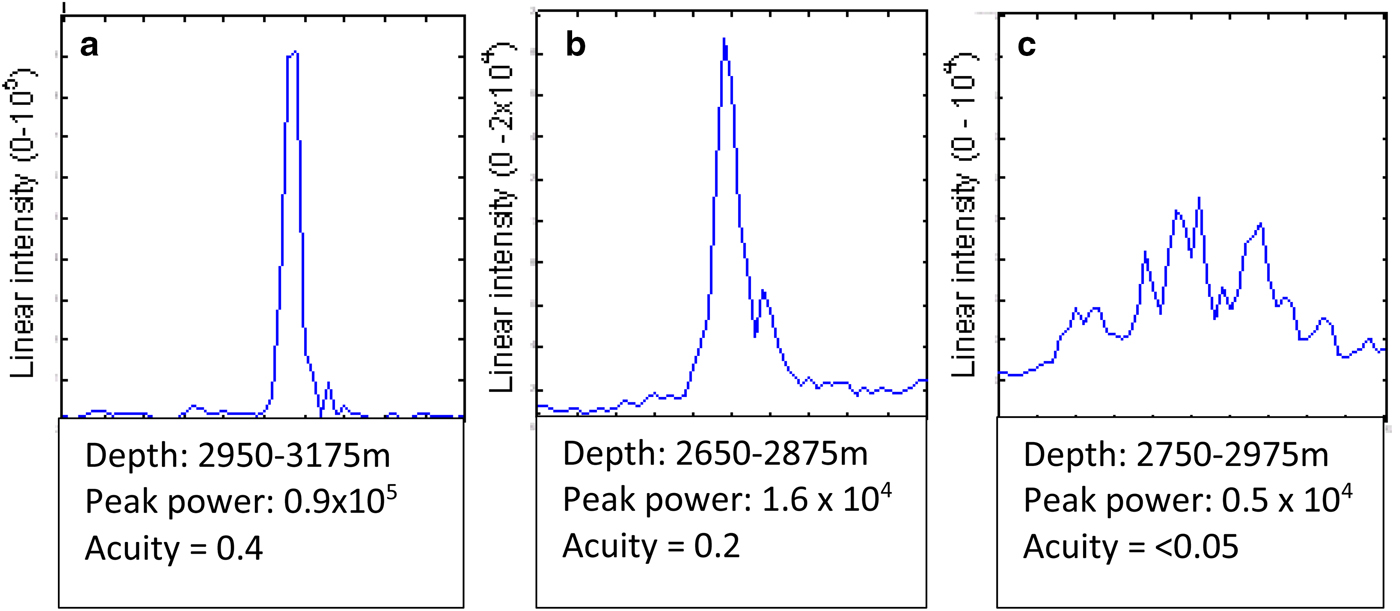
Different examples of the shape of the reflected signal envelope are illustrated in Figure 1. Where the reflection is close to specular, its duration is unchanged from that of the transmitted pulse (following pulse compression), which occupies ~2 radar range bins, yielding acuity <~0.5. As described above, reflections from a rough interface result in extended duration of the echo and variations in its peak amplitude. The acuity can be measured for every received pulse, and is found to range from 0.5 down to a value <0.05 for a surface where the TPIA is large and reflections are spread over a wide range of directions of arrival. Here we re-use a figure from Oswald and Gogineni (Reference Oswald and Gogineni2008), to provide a benchmark for comparison of the observable acuity with pulse shapes reported by Jordan and others (Reference Jordan2017) (Fig. 4) as a common starting position. Note that acuity of the radio echo signal is a less stringent constraint than that of specularity for the reflector.
Received signal envelopes from (a) a smooth bed, (b) a marginally smooth bed and (c) a rough bed (from the 1999 PARCA survey), at the pulse length scale. (Reprinted from Oswald and Gogineni (Reference Oswald and Gogineni2008), © J Glaciology.)
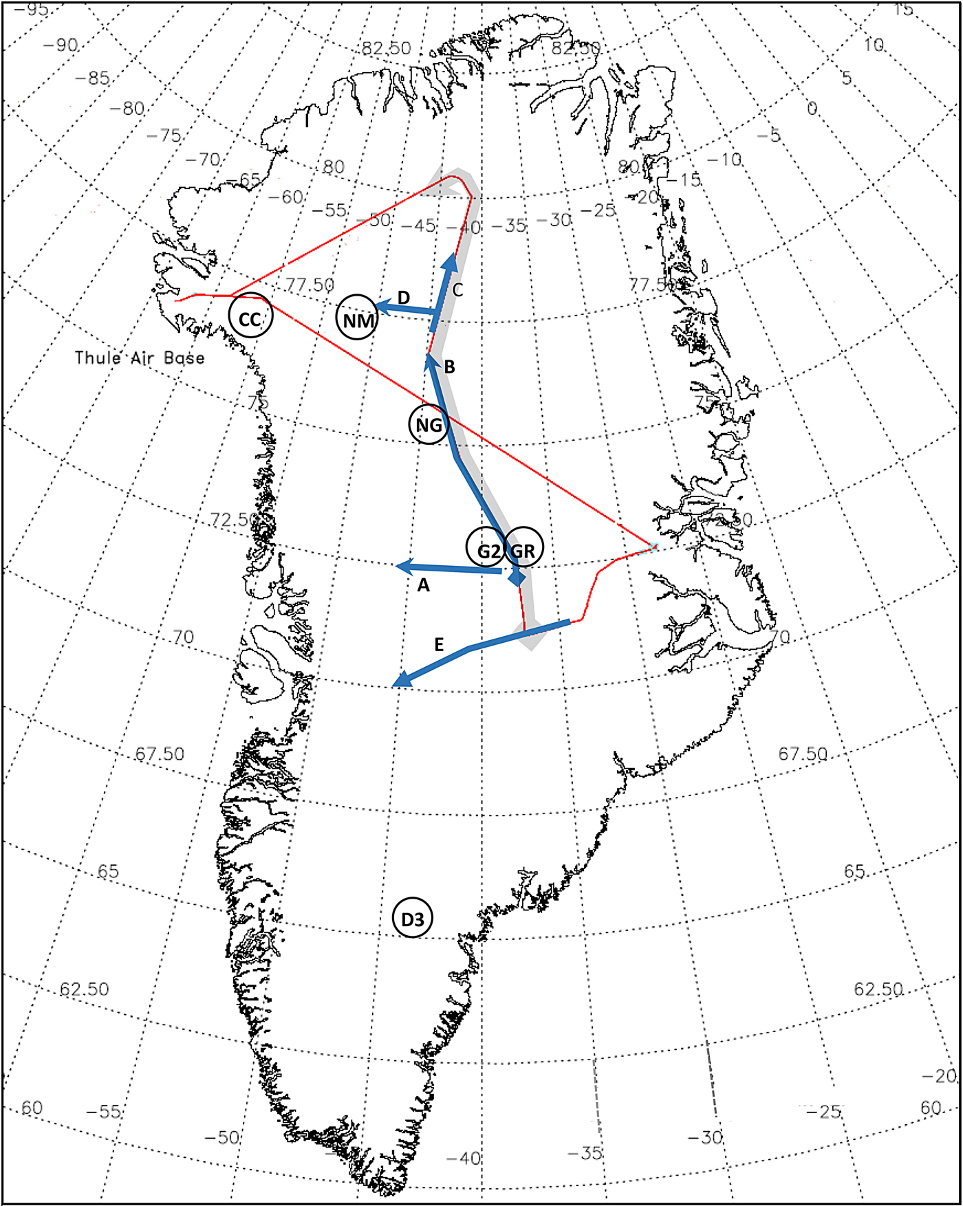
Flight segment examples from PARCA report, 1998, 1999. The red flight line is from 14 May 1999, with shorter segments from 23 and 25 May 1999 and 14 July 1998. Segment A covers 200 km, 23 May 1999. Grey segment (1160 km) includes ‘B’ (600 km) and ‘C’ (120 km) with differing bed conditions. Segment C and segment D, 25 May 1999; irregular internal layering and varying bed conditions. Segment E, 14 July 1998, illustrates differing internal layering, Section 3.5. Sites of core drilling to bedrock are circled: NEEM (‘NM’), Camp Century (‘CC’), NorthGRIP (‘NG’), GRIP (‘GR’), GISP 2 (‘G2’) and DYE-3 (‘D3’).
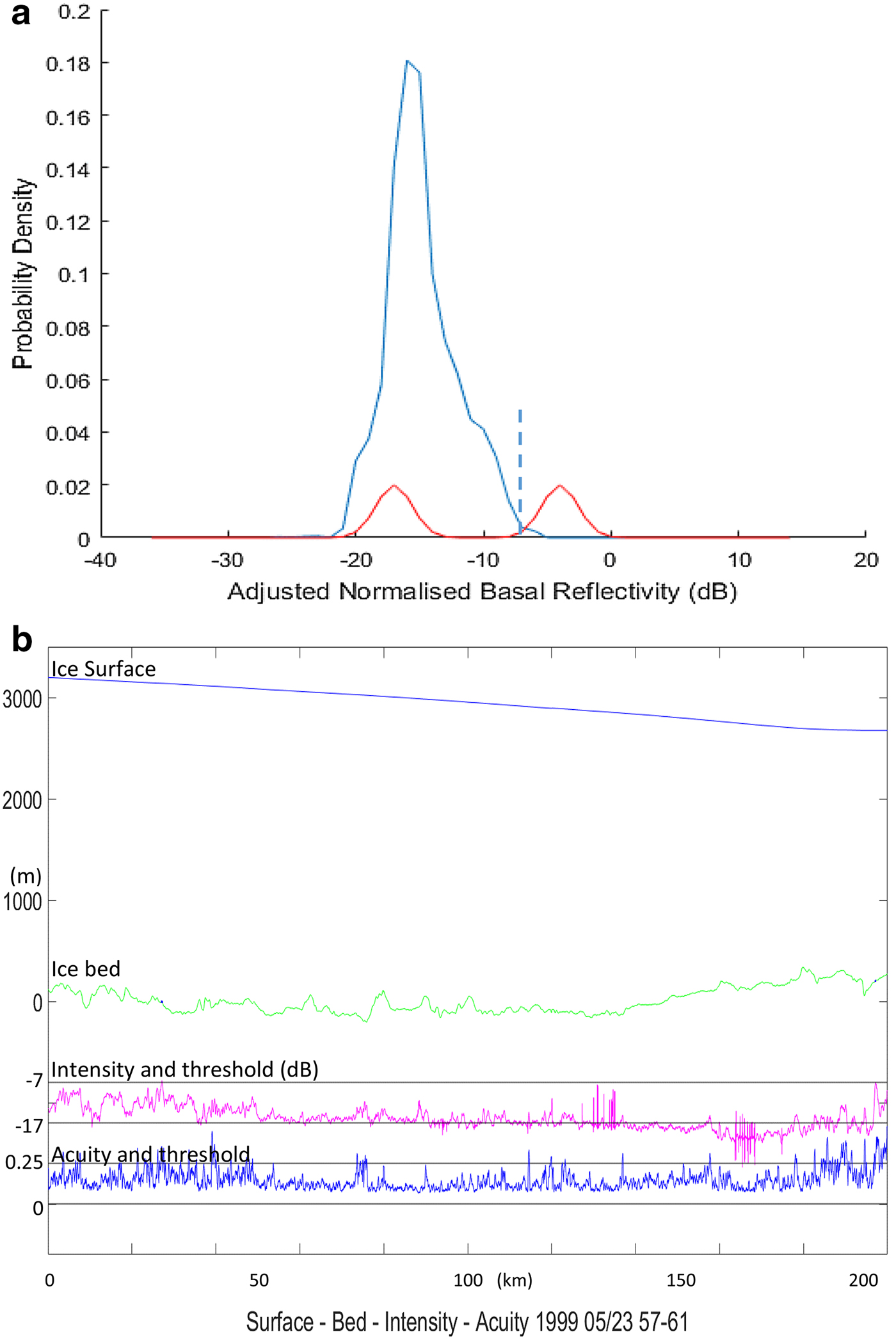
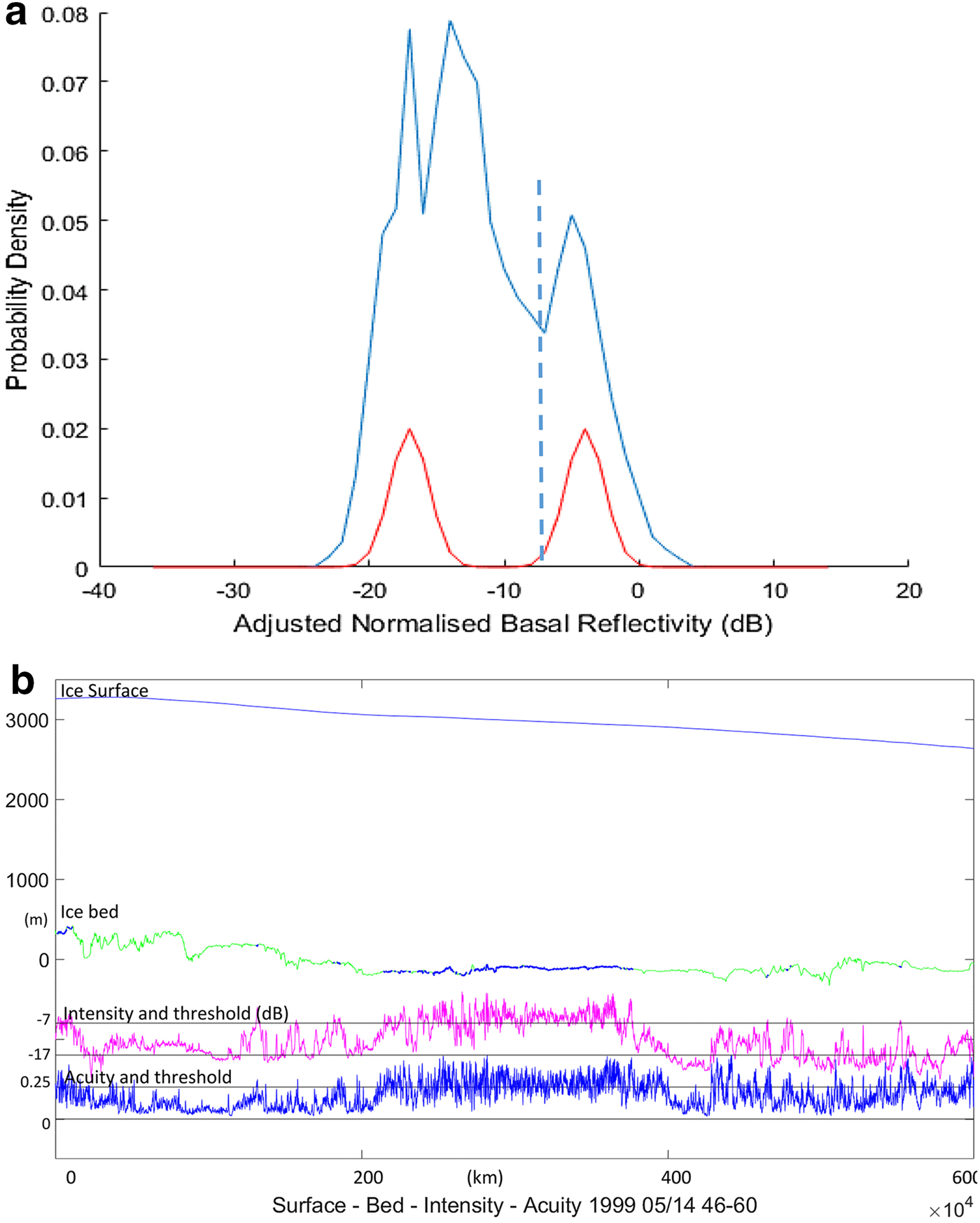
(a) Probability density of normalised reflectivity for flight segment A, plotted against reference curves for granite and water (red). The reflectivity reference is at −17 dB; the threshold is set at −7 dB. (b) Profile of the 200 km segment A in Figure 2, showing surface and bed elevations, intensity and acuity. The bed shows little evidence of ponded water. There are some fast intensity excursions typical of radio interference, which suppress the measured acuity.
(a) Probability density of normalised reflectivity at the bed for flight segment B in Figure 2, plotted against the reference curve. (b) Profile of the 600 km segment B in Figure 2, showing surface and bed elevations, normalised reflectivity and acuity as functions of distance. The bed starts without ponding at the left (south). Abrupt transitions between ponding and grounding occur before the flight traverses an extended thawed region (in which both parameters still vary rapidly up to high peaks) between 200 and 400 km, returning to a grounded bed and further rapid intensity transitions below the threshold. It yields the normalised reflectivity distributions shown in Figures 4a, 6, and the intensity/acuity histogram in Figure 5.
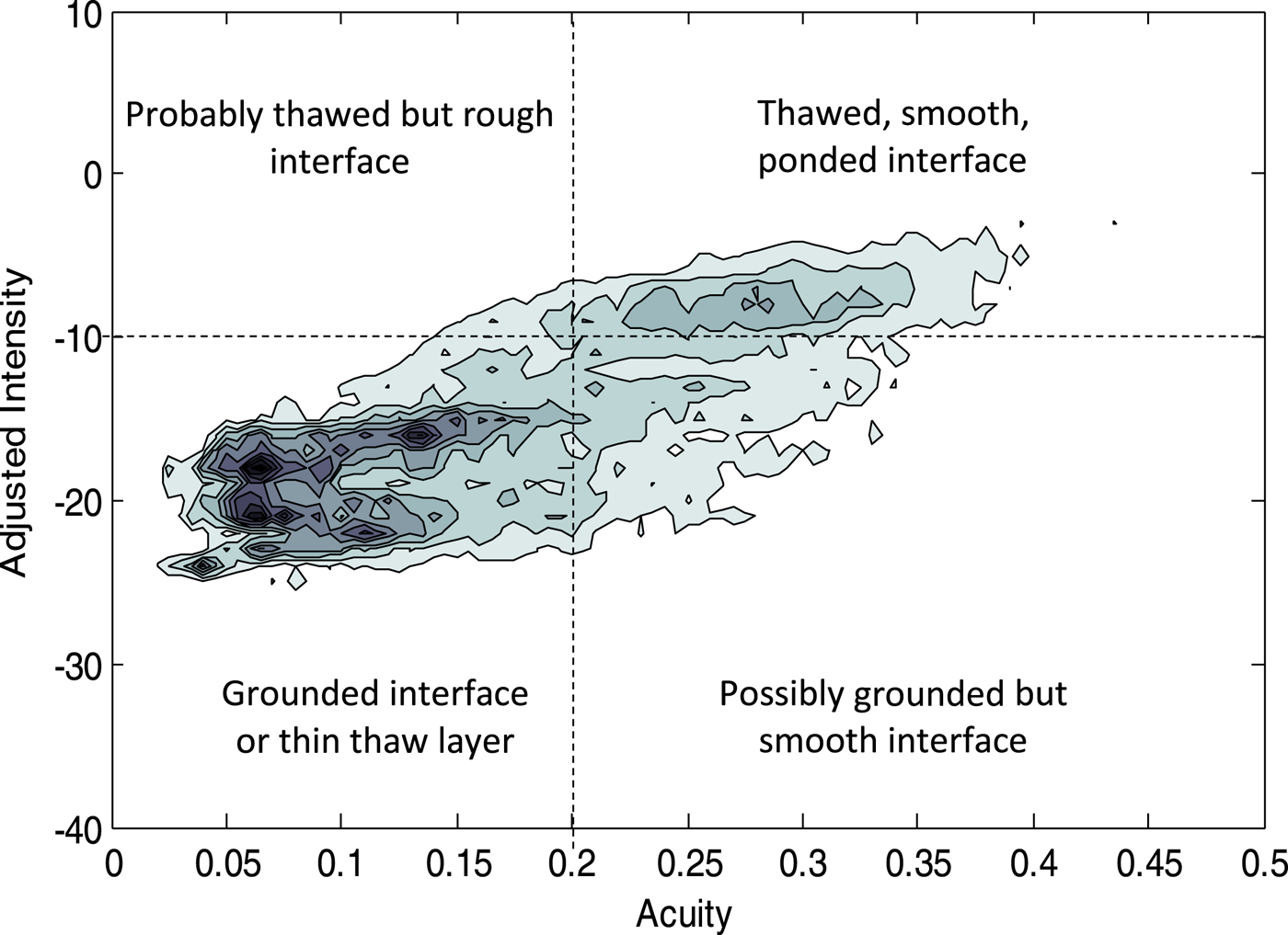
Two-dimensional histogram of reflection intensity vs reflection acuity for the same 600 km segment. Contours are at evenly spaced probability density values between 0 and 0.08.
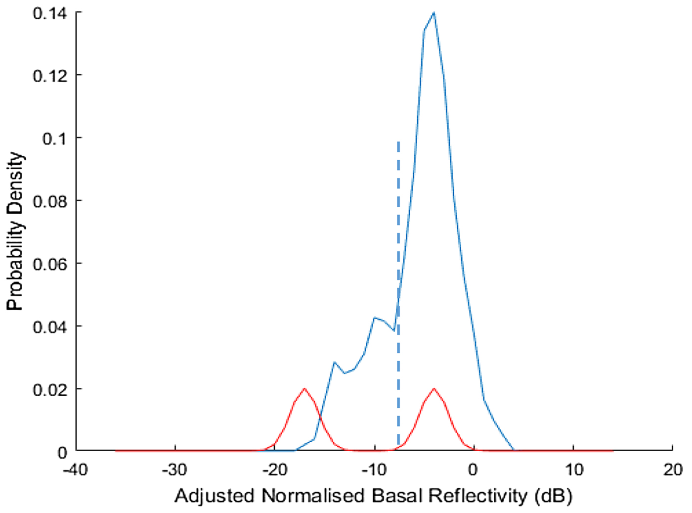
Normalised reflectivity distribution for the central segment of segment B, illustrating ponded thaw with a residual ‘grounded’ population below the threshold.
In combination with these geometric effects, interference occurs between the scattered signals, causing fluctuations in intensity or fading at spatial wavelengths of several metres or tens of metres along the flight path, at these depths and wavelengths. Fading introduces fluctuations in the peak intensity, but is conservative with respect to the mean intensity, and we average the received signal energy over a distance of ~200 m. Losses due to pulse extension are also conservative in that the reflected signal energy is dispersed rather than being absorbed, and are largely (but not precisely) recovered by aggregation over the received pulse length (see Oswald and Gogineni, Reference Oswald and Gogineni2008, Reference Oswald and Gogineni2012; Jordan and others, Reference Jordan2016), with accuracy in the region of 1 dB. Both the aggregation over pulse extension and averaging over fading are essential to adequately narrow the distribution of the signal intensity for rough interface reflections, and thereby to identify changes in reflectivity.
2.4. Material effects: reflection at the bed
In the discussion below, we re-visit the method for detecting variations in the mean aggregated basal reflectivity, including the use of knowledge of the possible range of bed materials; ice, water of various thicknesses, and rocks of various types.
The reflected waveform at a smooth ice–bed interface is related to that of the incident wave at the bed with intensity reduced by the reflection coefficient, which varies with the relative permittivities (ε r) above and below the interface. Ice has ε r ~ 3.2, and liquid water ε r ~ 80.
The relative permittivity for rock types to be found beneath the Greenland Ice Sheet can be found in several publications; for example, Hubbard and others (Reference Hubbard1997) (Table 2):
Relative permittivity for different rock types in saturated and dry conditions (from Hubbard and others, Reference Hubbard1997)
For materials of relative permittivity ε r1 and ε r2, the power reflection loss is given by
 $$L_{\rm ref} = \hbox{20} \times \,\hbox{log}((\sqrt {(\varepsilon _{\rm r1} )} - \sqrt {(\varepsilon _{\rm r2} )} )/ (\sqrt {(\varepsilon _{\rm r1} )} \; + \sqrt {(\varepsilon _{\rm r2} )} )),$$
and the effective radar cross-section is given by:
 $$ \eqalign{& \hbox{RCS} = \hbox{1}0\, \times \,\hbox{log} (L_{\rm ref} \times \; \pi \times (R(\hbox{TPIA})^{\rm 2})), \, \hbox{or} \, \cr & {\rm RCS} = \hbox{1}0\, \times \,\hbox{log} (L_{\rm ref} \times \; \pi \times (R(\hbox{ZF})^{\rm 2})),}$$
depending on the scale of basal roughness.
For an ice–rock interface, the reflection loss for these types, which in all probability comprise much of the Greenland Ice Sheet bed (Dawes, Reference Dawes2009) will vary from −13 dB for saturated basalt or limestone to −19 dB for granite, with a median value near −16 dB. Dry sands may yield a reflection loss below −25 dB, but we do not expect them to form a large part of the ice-sheet bed and have seen little such evidence.
For interstitial water at the radar frequency, the reflectivity ranges from −13 up to −3.5 dB for layers deeper than one-eighth wavelength in water; for the PARCA radar at 150 MHz, the change in reflectivity is substantial for water more than ~3 cm thick. We have set the ‘water’ threshold for the estimated reflectivity to a value of −7 dB, lying 3.5 dB below the expectation for ponded water and 6 dB above the upper bound for dry rock. The change in reflectivity tends to occur rapidly over short spatial scales greater than R(ZF), thus further differentiating it from being caused by other variations such as ice fabric or internal temperature, and their associated loss uncertainties. When combined with increased acuity of the reflection, this provides a further distinguishing feature of radar reflections as an indication of the bed material changing from rock to ponded water.
2.5. Material effects: dielectric absorption
The greatest loss in received signal intensity in radio-echo sounding occurs because of dielectric absorption, whose rate with depth is not independently known. However, for a change in reflectivity at the bed to become statistically significant, it is necessary to compensate for dielectric losses. At 150 MHz, over a fairly wide neighbouring spectrum, and with a surface temperature near −30°C, the average rate of absorption in deep ice may be over 15 db km−1 (one way), (Jordan and others, Reference Jordan2016): for ice over 3000 m deep, the total loss may be >90 dB. This effect depends on the ice thickness and on the englacial dielectric loss tangent, which is a function of temperature and chemical impurities. The loss is also increased by internal reflections due to changes in the properties of annual layers, but this effect is minor (e.g. MacGregor and others, Reference MacGregor2007). The loss tangent, averaged over the ice depth, may vary widely (e.g. Matsuoka, Reference Matsuoka2011). However, it can be expected to vary relatively slowly with distance along the sounding flight path, in correlation with slowly varying temperature profiles and deposits of impurities, and with changes in the ice fabric that are observed by proxy along the flight path in radio-echograms, typically over distance scales of tens or hundreds of kilometres (Figs 7b, 8a, an unusual example of irregular englacial layering).
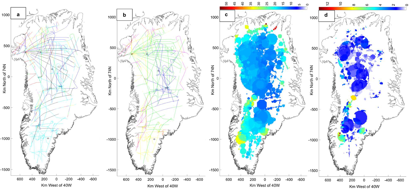
(a) Marginal rates of dielectric absorption through the ice column as fitted along each flight segment (colormap ‘jet’ coding <5 to >30 dB km−1). (b) Mean absorption rates through the ice column found by reference to the grounded ice/rock reflection coefficient. (c) Mean absorption rates as extrapolated through continuity zones. Mean over the ice sheet = 16.6 dB km−1. (d) SD between absorption rates where more than one measurement is available. SD over the ice sheet = 2.3 dB km−1. In summary, the absorption rate is within the expected range and is seen to increase from the high central dome towards the coast, and from north to south. Deviations increase towards the coast, and large central areas exhibit SD well below 2 dB km−1.
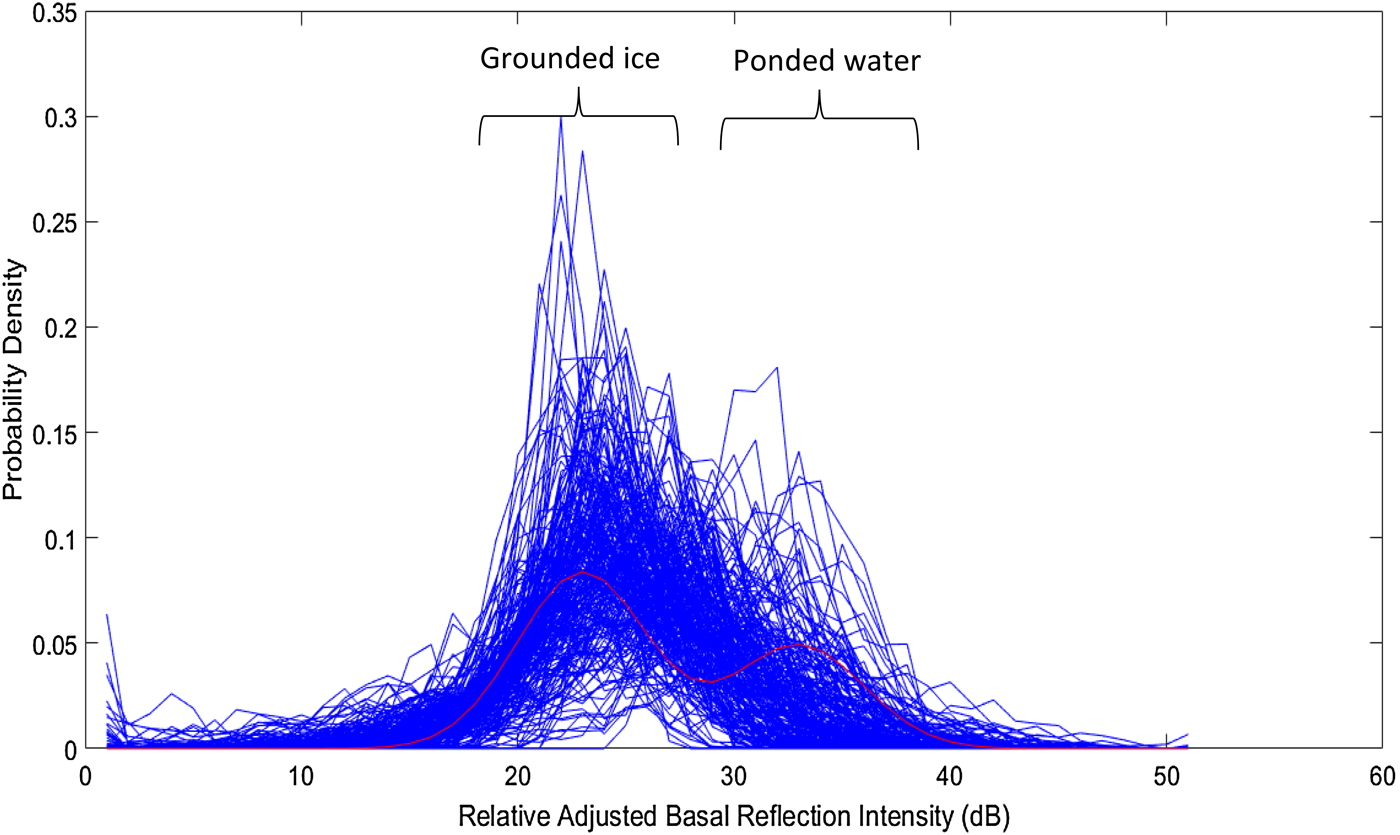
The distribution of signal intensity after adjustment for dielectric absorption, but pre-normalisation, measured over the total flight path 1998–2003.
Where the ice depth and the flow pattern vary rapidly along the flight path, greater variability in the loss tangent may be expected and can cause errors in the marginal rate of change with depth along the flight path. This uncertain rate of attenuation by absorption, even if slowly varying with position, requires us to seek a better reference point for the basal reflectivity as discussed in Section 3.
2.6. Resolving uncertainties in dielectric absorption
Matsuoka and others (Reference Matsuoka, Morse and Raymond2010a, Reference Matsuoka, MacGregor and Pattynb) conclude that modelling the absorption in the ice column based on prior models of composition and temperature results in considerable uncertainties, and that the residual loss ascribed to reflectivity must therefore be similarly uncertain. Such uncertainties are quoted by Jordan and others (Reference Jordan2017).
However, the reflectivity at the ice-rockbed, as described in Section 2.4 above, is itself a much better understood variable (based on the known, limited variability between rock types) than the modelled total englacial dielectric absorption. A more robust reference is provided by the dielectric characteristics of subglacial rocks themselves, as shown in Table 1 (Hubbard and others, Reference Hubbard1997; Dawes, Reference Dawes2009), which are known to be present and to occupy the majority of the ice-sheet bed. They have provided robust bed reflections for the great majority of radio-echo surveys, for which the suggested variabilities in englacial absorption would have proved unmanageable.
To compensate for the effect of absorption on the observed signals, we first make allowance for the known geometrical spreading loss, and find the best-fit marginal attenuation rate (d(L abs)/dz)fp with depth along each flight path segment, whose application minimises the variance of echo intensity and its correlation coefficient with ice depth for that segment. Dielectric losses always reduce the signal intensity. However, when the flight path crosses an area in which the loss increases proportionately less rapidly than the depth (e.g. where the flight path crosses a glacial flow and the depth increases as the ice temperature falls), the apparent marginal loss rate (dL/dD)fp, measured along the flight path, can indeed become negative. We demonstrate that the residual intensity distribution over large areas can be narrowed to the extent that excursions in intensity are found to be consistent with such rocks or with a mix of rock and ponded thaw, and that, where a mix is apparent, are correlated with signal characteristics (the acuity) known to be related to the bed rather than to the ice column.
After narrowing, the distribution of intensity is normalised (shifted on the logarithmic scale), based on our knowledge of the range of bed materials. We find that the distribution of intensities closely matches the range of reflectivities expected from the known range of materials. With exceptions such as during aircraft turns, radio interference or extreme disturbances in the ice column, we find very broadly that the lower peak of residual intensity has a standard deviation (SD) of only ~3 dB. However, it exhibits upward excursions, which are not correlated with depth, with an upper bound ~10–15 dB higher.
Flight segments are extended until a single value of d(L abs)/dz fails to narrow the variance sufficiently to resolve the reflectivity of components of the population with SD of ~3 dB and a mean deviation of ~10 dB.
Extended flight segments vary from 40 to 1200 km in length.
Taking this ‘Bayesian’ approach to the reflection statistics (using the distribution of probable reflectivities as the prior reference), we use the radar data to select between the known characteristics of ice/rock and ice/water interface configurations, rather than relying on the uncertainties in estimating the total absorption to calculate a small residual. We determine where the ice-sheet bed includes a more strongly reflecting component and, independently, where the signal acuity is high, representing a relatively smooth bed. We determine therefore whether the apparently high reflectivity coincides with high acuity, known to be directly associated with the bed itself. This coincidence is taken to indicate that a reflective layer of water is present at the bed.
Mathematically, this procedure is equivalent to the difference equation:
 $$\Delta (\hbox{SNR})/\Delta x = \Delta (\hbox{RCS})/\Delta x - \Delta ^{\rm 2}(L_{\rm abs})/\Delta x,$$
where RCS is proportional to reflectivity as in equations (8). Δ2(L abs)/Δx represents the mismatch of the absorption loss with the linear compensation factor used over the segment. It is expected to be uncorrelated with changes in the bed reflectivity and therefore to be bounded as a maximum by the SD of the features of the intensity distribution. Where this SD is sufficiently narrow, and where the total intensity distribution has sufficiently steep lower and upper bounds, the distribution then provides an estimate of the distribution of reflectivity.
2.7. Distinctions between acuity and specularity
The method used here has also been subject to question concerning the connection between basal roughness and reflectivity (Jordan and others, Reference Jordan2017). In a study of radio-echo surveys in northwest Greenland (under Operation IceBridge) a parameter, the Hurst exponent (H), is introduced that is related to the scale variation of basal roughness as measured by the radar (at scales above tens of metres). It can be used to model radar scattering, and takes a minimum value near zero for highly specular reflecting interfaces. The authors show, according to their Figure 7, that smoother reflecting interfaces as indicated by higher mean values of the acuity of the radar reflection are associated with areas of low H, in which the vertical scale of roughness increases only slowly with increasing horizontal scale. This is in agreement with our method and expectation. However, in comparing the nature of the roughness statistics in this local area of Greenland with predictions of basal thaw from both MacGregor and others (Reference MacGregor2016) and Oswald and Gogineni (Reference Oswald and Gogineni2012), in their Figure 8 they find a contradiction: areas predicted to be thawed by the numerical model tend to exhibit greater values of H and lower acuity than areas predicted to be frozen.
This finding is also counter-intuitive with respect to the reflection process. While Oswald and Gogineni (Reference Oswald and Gogineni2012) did not assume that basal thaw in Greenland consisted of specular reflectors as found in Antarctica (which would yield values of Ac of at least 0.5), they conjectured that values of acuity would tend to be higher for water-filled subglacial ponds, which, given the higher density of water vs ice, will indeed tend to acquire a more planar upper surface, bounded by rough features of the interface. The condition of high specularity, which operates at the wavelength scale and is equivalent to ‘coherence’, for which high values have been encountered in Antarctica but in very few locations in PARCA radar results, is very much more stringent as a criterion than that of acuity, which operates at the (larger) compressed pulse length scale.
In comparing H values with other radar results, we would rely on Jordan's Figure 7 with respect to H and Ac. We acknowledge that earlier radar results overstated ponded thaw in the northwest of Greenland; however we do not agree that rougher areas are more likely to be thawed, despite possible disagreement with certain models. Our analysis of ponded and grounded areas is provided in Section 3, with mapped results, discussion and comparisons in Sections 4 and 5. We anticipate that these may reduce any contradiction between basal thaw findings and the Hurst exponent.
3. MEASUREMENT METHOD AND EXAMPLES
The method for detecting ponded subglacial water is based on measuring radar signal characteristics that represent the condition of the ice-sheet bed as it affects the reflection of radio echoes.
We adjust the apparent englacial attenuation rate to minimise the residual SD of the received echo intensity over distances varying from tens to hundreds of kilometres, and normalise it to the range expected from the available bed materials. We find that this procedure leads to well-constrained intensity distributions over large sample populations. There is typically a dominant fraction of echoes that exhibit relatively low adjusted intensity, with SD in the region of 3 dB. However, in a significant minority of cases, there is a secondary fraction, in many cases clearly distinct, with higher intensity but matching the expected range of values for ponded water by comparison with the rock-bed, revealing changes in the bed reflectivity.
Figure 2 maps a number of flight segments from 1998 and 1999, used below in discussion of these observations and the robustness of our interpretation.
3.1. Narrowing the distribution of intensity
We start our analysis with an example from a survey flight on 23 May 1999, which provides a large measurement population with a range of surface elevations and bed topography, and an earlier flight on 14 May 1999, with an even larger population and a range of latitudes, with ground truth data from GRIP and NorthGRIP coring sites. The flight paths are illustrated at A and B in Figure 2, and provide a measurement population with over 6000 degrees of freedom, based on the number of independent measurements from 33 × 40 km flight segments.
Segment A illustrates the intensity distribution obtained for a typical flight segment where water is not indicated. After minimizing the intensity variation related to depth, using the single marginal absorption rate of 21 dB km−1 (one-way) and normalizing at the low margin, the residual reflectivity distribution, covering 200 km of the flight, is shown in Figure 3a. Its elevation and depth profiles, and intensity and acuity profiles, are shown in Figure 3b.
In following figures illustrating profiles of the ice, the surface is represented by a blue line, the bed elevations (green line), the echo reflectivity (magenta) and acuity (dark blue), with water ponds superposed in dark blue on the bed trace. The reflectivity reference is at −17 dB and the threshold at −7 dB. Acuity references are at 0 and the threshold at 0.25.
3.2. Examples of profiles, echo intensity and acuity
Figure 4a shows the intensity distribution for segment B in Figure 2, after compensation for an absorption rate of 11.5 dB km−1. Transitions in bed echo intensity within a ponded bed tend to occur over spatial scales longer than typical fading patterns (10 m to over 100 m), but shorter than the larger scale topographic relief that affects absorption losses; however, no spatial-frequency filtering has been applied. These transitions that occur over hundreds of metres and recur over tens of kilometres illustrate that the variations are driven by factors at a smaller spatial scale than variations in topography. They are not conservative (i.e. they are not eliminated by averaging or by aggregation over the received pulse length), and therefore are not due to fading or roughness at this scale. They represent a persistent change in reflected intensity with short-scale fluctuations.
Figure 4b shows the same variables as in Figure 3b, for segment B, which is chosen to illustrate a range of bed conditions.
For the 1120 km segment (shadowed grey in Fig. 2) which includes segments B and C, a single marginal attenuation rate (11.5 dB km−1, one-way) is used and adjusted in the same linear way as Oswald and Gogineni, Reference Oswald and Gogineni2008, with latitude and surface elevation.
This flight segment is recorded in 150 000 successive radar range scans. Taking the scale of independent measurements as the diameter of the First Fresnel Zone (~120 m), the 600 km flight segment contains ~5000 independent samples that compose the histogram population in Figure 4a. The population to the left of the dotted boundary contains ~3800 samples and that above, 1200. This distribution is well-matched by the sum of two Gaussian populations differing by 11 dB in their mean values, with SD close to 5 and 3 dB, respectively, and standard error <0.2 dB. A Student's ‘t’ test of the data yields a confidence level better than 99.9% that two separate populations are present.
This separation is consistent with variable bed reflectivity, but in itself is not sufficient to exclude the alternative possibility of two conditions of the ice column with different absorption coefficients. To resolve this ambiguity, we can compare such results with the bed reflection acuity, as derived in Section 2.3. The acuity is determined by the small-scale local topography of the ice-sheet bed, and not by the medium through which it has travelled. Positive correlation between the signal intensity and the acuity therefore is evidence that the intensity is also a function of the bed material.
In order to test the degree of correlation between the echo intensity and its acuity (known to be determined locally by the bed), in Figure 5 we plot a two-dimensional histogram of the population density against the intensity and the acuity, for this 600 km flight segment B.
The horizontal trends in the histogram are direct evidence of narrow intensity distributions for at least two distinct population fractions. The higher density (darker) peaks are clearly differentiated both according to the reflection intensity and to the acuity, and therefore to the local nature of the interface. They illustrate the effectiveness of the process of averaging and summing the echo intensity, yielding narrow ranges of intensity within each fraction. Reflection acuity varies from <0.05 to ~0.4, as expected.
There are two or more distinct populations along the intensity axis; the lower fraction (which itself appears to consist of two or more narrow intensity peaks) has an SD close to 5 dB, as against 3 dB for the higher intensity fraction, with a mean difference of 9–15 dB between the populations. Figure 5 also illustrates that the observed correlation of reflectivity with acuity is consistent with the expected difference between a direct ice–rock interface yielding reflections at −25 to −13 dB (for acuity 0.05–0.2), and a ponded, water-intruded interface yielding −12 to −5 dB (for acuity 0.22–0.4). For a population of this size (>5000 degrees of freedom), there is a likelihood <0.1% that this histogram represents a single random population dominated by uncertain absorption rates, uncorrelated with the bed condition.
We find that changes in the apparent bed reflectivity tend to be positively correlated with changes in the acuity value, strongly supporting the case that variations in the intensity, after adjustment for slowly varying geometric and dielectric losses, are indeed related to the interface itself rather than to uncertainties in englacial attenuation, which are expected to be independent of the interface roughness.
We therefore interpret the compensated intensity as being directly related to the reflectivity of the boundary and therefore to the presence of reflective, ponded water. In Bayesian terms, our prior information about these materials, when combined with the variations observed in both intensity and acuity, supports an interpretation in terms of basal ponding.
The concern that this radar method is likely to yield false delineations of ponded/grounded beds for this reason can therefore be discounted, but only with respect to subglacial water layers over 3 cm deep. Very thin layers of water or areas of wet till are likely to be assigned by this method to the ‘grounded’ fraction, leading to a distribution of ponded water that understates the total area of basal thaw.
For completeness, Figure 6 illustrates the intensity distribution for the central 200 km of track B, in which ponded thaw is found to be effectively continuous. There remains a ‘grounded’ fraction at the lower intensity end of the distribution, as is almost always the case.
In all of these cases, the process of compensation for variable absorption loss has resulted either in a narrow distribution with SD near 3 dB, or a composite distribution with a range of constituents of similar width over the flight segment.
We conclude, based on the successful reduction of depth-related intensity variance and the incorporation of known constraints on bed materials and scattering processes, that the evidence of internal consistency in the results, the observed (but not exclusively) positive correlation between acuity and reflectivity, and the broad external validity with respect to known glacial features such as the North East Greenland Ice Stream (NEGIS), that these observations are well-founded. As a further example for comparison with Figure 3a, we include a radio-echogram at Figure 9a of a segment from 25 May 1999, whose profile is shown in Figure 9b, in which the reflectivity changes rapidly several times in good correlation with the acuity while the ice shows considerable internal disturbance.
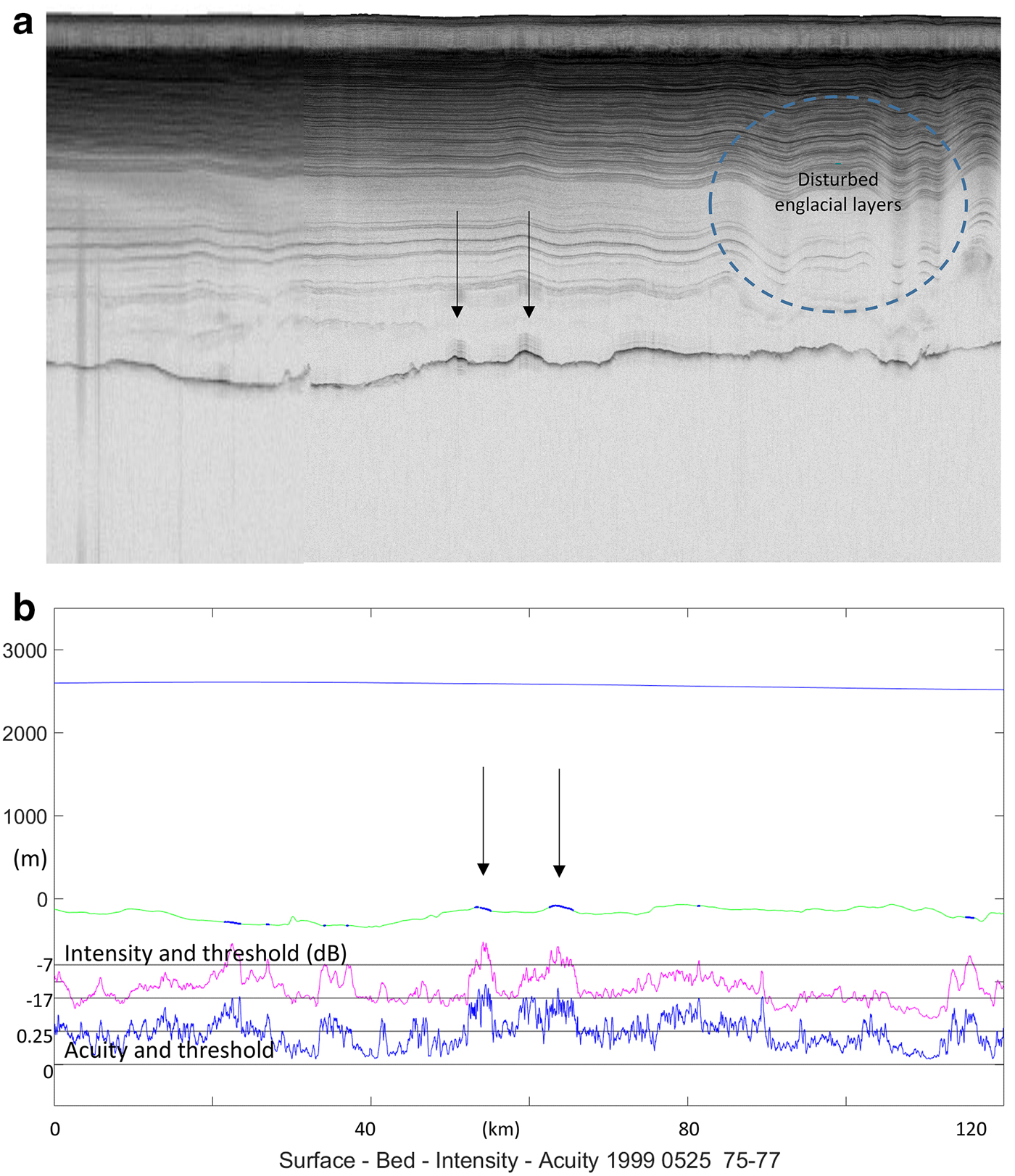
(a) PARCA radio-echogram for segment D, Figure 2, indexed horizontally with Figure 9b, illustrating bed and internal layer echoes in relation with indicated (↓) thaw ponds/channels, which may be incised upwards into the ice. (b) Radio-echo ice profile for segment D (Fig. 2) with intrusions of ponded water.
There is one further possibility of mistaking the nature of these changes in reflectivity. The presence of a low-permittivity (ε r ~ 3.5–4) fraction, such as sand forming a rough interface, with intrusions of smoother, high-permittivity but dry rock such as limestone (ε r > 7), could provide similar reflectivity and acuity contrasts to those between say granite and ponded water, resulting in misclassifications. However, if water was also present in such an area, we would observe contrasts in mean reflectivity of well over 20 dB. We have found no such instances. For such occurrences not to occur, it would be necessary for all areas with ponding to be geographically separate from areas with such a low-permittivity fraction, which we consider to be not impossible, but very improbable.
3.3. Normalisation of the distribution of intensity
We have focused on the intensity and acuity of the bed reflection caused by the discontinuity between ice (whose loss tangent varies with temperature and impurities but whose permittivity is narrowly bounded) and rock (a material with several well-characterised and similar permittivities), whose reflectivity is narrowly bounded by comparison with englacial dielectric losses.
We wish to identify the nature of the bed and its allocation between (a) typical rock types of permittivity between 5 and 8, yielding low reflectivity, or (b) such rock overlain by a layer of water more than 3 cm deep, with permittivity close to 80, with a higher reflectivity. Only in the case of an ice shelf would type (b) dominate the bed characteristics, and the known topography of the GIS precludes that case.
For the Greenland Ice Sheet, type (a) is likely to be the dominant class, consisting of metamorphic, sedimentary or igneous rocks (Dawes, Reference Dawes2009), with or without a negligibly thin thaw layer, yielding low reflectivity. Class (b) is where the bed is substantially thawed and ponded, and where the well-known characteristics of water will dominate and provide substantially higher reflectivity and a relatively smooth interface. The lower peak in these histograms, for example, in Figures 3a, 4a, with a sharply rising lower bound and peak, provides a common feature for almost all the compensated radio-echo intensity distributions, and is set as a normalising baseline of reflectivity for all the bed echoes, near −17 dB and representing the grounded state. Using this baseline, and after narrowing and normalising the intensity distribution, we search for excursions above the reflectivity threshold of −7 dB. We find almost universally that such excursions are associated with raised echo acuity, linking them with the local ice bed topography, and we have used this condition to identify ponded water within each flight segment. Naturally there are also excursions in acuity, representing a smooth bed, that are not linked with high reflectivity, and which are not interpreted as ponds.
Taken together, these observations are difficult to reconcile with the finding of Jordan and others (Reference Jordan2017) with respect to the Hurst exponent and the reflective state of the bed derived from models.
In the course of setting the marginal rate of absorption with ice depth to minimise the observed range of intensities along a flight segment, and of normalising the narrowed distribution to the range of expected reflection coefficients, the process has yielded values both for the marginal rate of change of intensity with ice depth, and the mean rate of absorption with depth through the ice column.
The relation between the marginal rate of attenuation along the flight path and the mean rate integrated through the ice volume depends on the three-dimensional ice stratigraphy and temperature distribution, and the flight path across it. Figure 7a shows the marginal rates as fitted with depth variations along the flight paths, and Figure 7b shows the mean absorption rates as measured through the normalisation process. The marginal rate is more variable than the mean rate.
No mathematical windowing function has been applied to these segments of constant marginal absorption rate (which average 195 km in flight length), other than the finite length of the segment itself.
In Figure 7c, we have plotted the mean rates over areas where continuity of a grounded or thawed bed has been identified (see Section 4 below), and in Figure 7d, we show the SD where more than one estimate of the absorption rate is available.
The average over the whole survey area of the mean absorption rate through the ice column is 16.6 dB km−1, in good agreement with Jordan and others (Reference Jordan2016). Where crossovers occur between different flights and continuity zones, the SD is found to be 2.23 dB km−1, providing broad support for the robustness of this method.
The distribution of adjusted reflection intensity over the entire flight path during 1998–2003 is shown in Figure 8, which includes the distributions for all segments in Figures 7a, b.
3.4. Irregular topography
Where the bed topography is irregular, it is necessary to check the correlation of echo intensity with bed topography over distances of tens of kilometres. For example, near to the site of the Camp Century ice core, where the temperature close to the bed had been measured at −13°C (Weertman, Reference Weertman1968; Dansgaard and others, Reference Dansgaard, Johnsen, Møller and Langway1969), the bed reflection intensity and acuity incorrectly suggested the presence of ponding. This measurement at Camp Century alone showed that the use of a single parameter value over the whole ice sheet in the earlier analysis was of limited validity. Provision has now been made to vary the marginal absorption parameter, as described above, to compensate the bed reflection for observed correlations of intensity with depth within each 40 km flight segment. This provision has reduced the apparent presence of water in the north of Greenland (cf. Oswald and Gogineni, Reference Oswald and Gogineni2012), but retains key geographic features and is considered to be appropriately conservative.
Figure 9a (Section 3.4) shows a radio-echogram for segment D in Figure 2, and Figure 9b shows these variables after compensation at 15 dB km−1. Reflectivity transitions remain rapid and recurrent, but are less persistent. They correlate well with acuity, and meet the criteria for thaw ponds over distances of 1–3 km. Their convex vertical profiles raise a question about their hydrological nature; however, their intensity and acuity vary within these distances and may indicate the presence of many smaller ponds within shallow cavities in the interface, rather than of a single, convex upper surface. There are many and various features that suggest further opportunities for study. In this case, a few kilometres away, there is a further pond that is associated with significant disturbance in the internal layering, whose downward curvature suggests the possibility of substantial loss of ice at the bed; the range of possibilities is wide and beyond the scope of this investigation.
3.5. Irregular internal layering
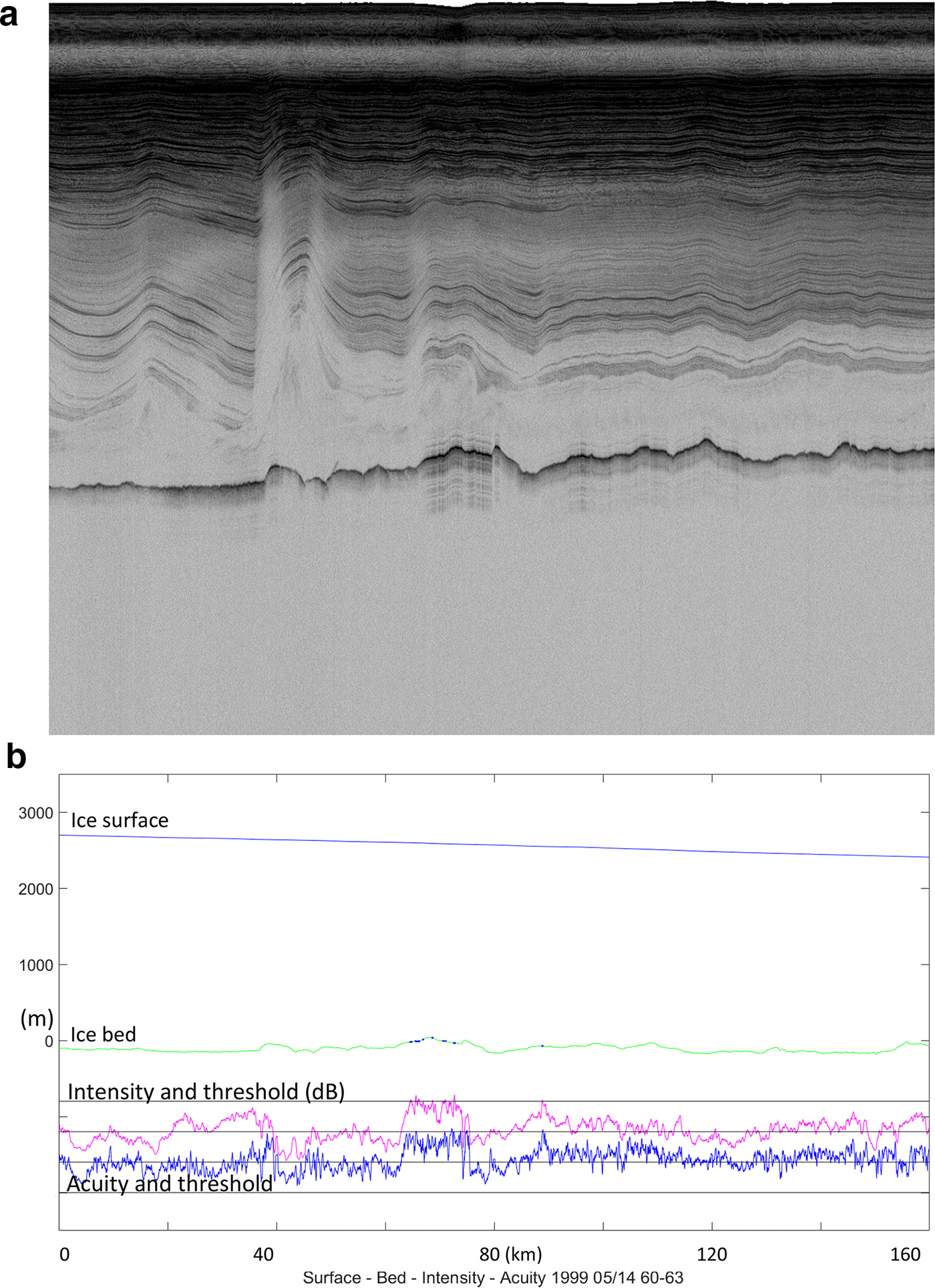
Radio-echoes from internal layering may provide evidence about the state of flow of the ice sheet. However, since the flight direction is not in general aligned with the ice-sheet flow lines, care is needed in any interpretation. In Figure 9a below, over the first 80 km, the echoes representing internal layers are notably steady in depth, whereas from 80 to 120 km, the layers are much more disturbed. Figure 10a illustrates more extreme layer disturbance with some bed features. Figures 9b, 10b illustrate radio-echo profile data in a similar format to the earlier profiles. The distinction of what appears to consist of thaw ponds from the surrounding rock is clear in both the intensity (magenta) and the acuity (blue) plots; however, there is substantial disturbance of the internal layers, with only a fractional disturbance of the intensity or acuity plots.
3.6. Conclusion on measurement
Our measurement challenge has not been to estimate the absolute reflectivity based on unknown conditions of absorption. The solution has been to normalise the depth-decorrelated variance of the averaged, aggregated bed reflection intensity, by reference to bounds based on the reflectivities of a known range of materials at the boundary with fresh water ice. We assign each point of the bed either to a grounded fraction (where the ice is in near-direct contact with bedrock, but may be at the pressure melting point), or to a ponded fraction, where the bed also exhibits enhanced reflection acuity.
This method avoids the dependence of the radar reflectivity measurement on prior knowledge of the englacial absorption rate, and therefore the concern that incorrect bed assignment may occur because the characteristics of the ice column are unknown or subject to short-scale variations.
In the following measurements and maps, we assign the bed state as ‘grounded’ or ‘ponded’ because the signal intensity is negatively correlated with ice depth, with a residual SD of ~3 dB and is found to vary locally with a mean deviation of typically +10 dB that is positively correlated with increased smoothness of the bed; the bed is shown to consist of two fundamental populations differing in reflectivity by ~10 dB; we know that subglacial water is expected and was encountered at the bed at NorthGRIP; we observe signals and distributions that are consistent with these expectations and with the presence of water, ponded to a significant depth (>~3 cm), and in very few cases do we observe variances that substantially exceed these levels after decorrelation with depth.
4. DETERMINATION OF BASAL PONDING IN GREENLAND
The determinations of ponded basal water arising from this analysis of radar flight data during 1998, 1999, 2002 and 2003 are illustrated in Figure 11.
Flights during the PARCA programme in 1998, 1999, 2002 and 2003. Cyan lines indicate a grounded bed: black lines a ponded bed. Narrow flight line widths are necessary to separate neighbouring paths. Ice core sites are initialled.
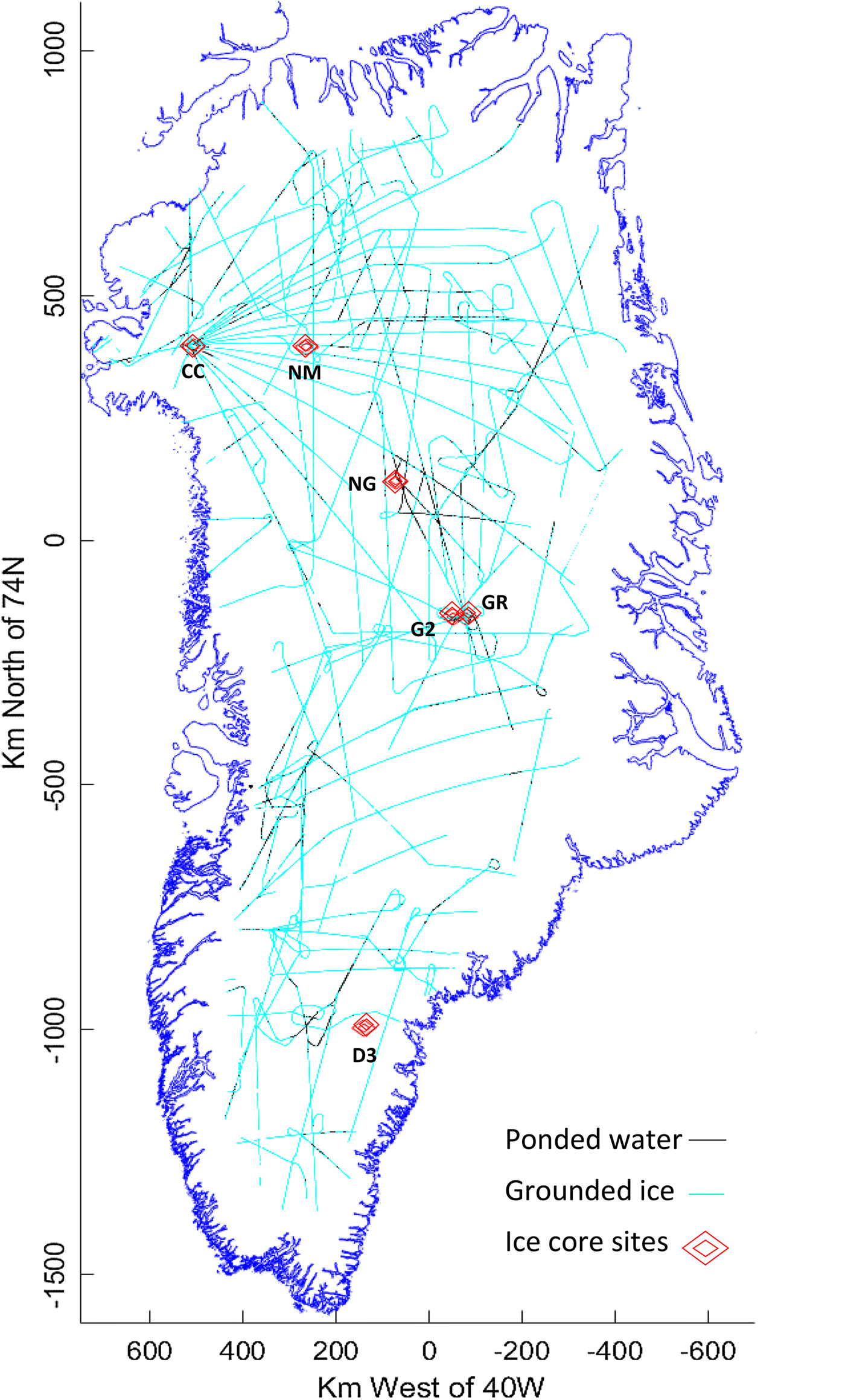
The flights undertaken during these four survey years cover a large portion of the ice sheet with spacing in the order of 50–100 km, while the path width over which the bed is actually measured is determined by the First Fresnel Zone/Pulse Illuminated Area. At ~60–500 m, this is narrow on the geographical scale, so that the immediate coverage represents only a little over 0.1% of the whole area. We therefore interpret these samples in the light of the following larger scale observations of the survey, which help us to extrapolate and interpolate between observations:
(1) The thickness of the measured ice sheet (~1000–3200 m) is such that the ice depth changes only by small fractions due to bed topography within the great majority of flight segments.
(2) The high degree of continuity of the surface elevation within and between flights, despite the wide flight separation (0–100 km) suggests it is reasonable to apply the continuity rules between as well as along the flight paths, and this is tested in terms of internal consistency.
(3) The scale of topographic features along the flight path (ten to hundreds of kilometres) show that bed features are large compared with the illuminated area and the averaged spatial sample spacing.
(4) The scale of the effective illuminated area (60–500 m) and the separation of independent averaged signal samples (~200 m) show that bed features are well sampled.
We also make an assumption that there will be, on average, no preferred alignment between flight direction and any unknown anisotropy in basal thaw features whose scale is too small to be adequately sampled by the flight pattern. This assumption will necessarily incur errors in the shape of subglacial thaw features at small scales, but allows us to make extrapolations that on average can be expected to represent the bed condition in a given broader area.
4.1. Interpolation of occurrences of subglacial water along the flight path
To make practical use of this information, we require an estimate of the presence or absence of ponded water (the ‘bed condition’) at any point in a grid covering the observed ice sheet. This requires an interpolation scheme between the flight lines. We do this by establishing a scale of ‘effective continuity’ of the bed condition (ponded or grounded) along each flight line. Points of ponded thaw separated by less than the ice thickness are assumed to represent continuous conditions for thaw in between, since, by inspection of many ice profiles, and except in extreme cases, significant changes in ice depth and internal layer patterns rarely take place over distances less than the ice thickness. Figure 10b illustrates a typical deep ice profile, whose vertical scale is exaggerated by a factor of over 10:1. Isolated pockets of thaw are found at a scale of fractional kilometres, separated by many kilometres, and are not extrapolated. Significant thaw tends to set in over distances of 2–10 km.
Where detections of thaw are separated by more than the ice thickness, the intervening path is assumed grounded (i.e. no ponded water detected). The scale of effective continuity for thaw is determined by the distance over which all the separations are less than the ice thickness, while grounded segments extend where thaw points are absent or more widely separated.
4.2. Interpolation between flights
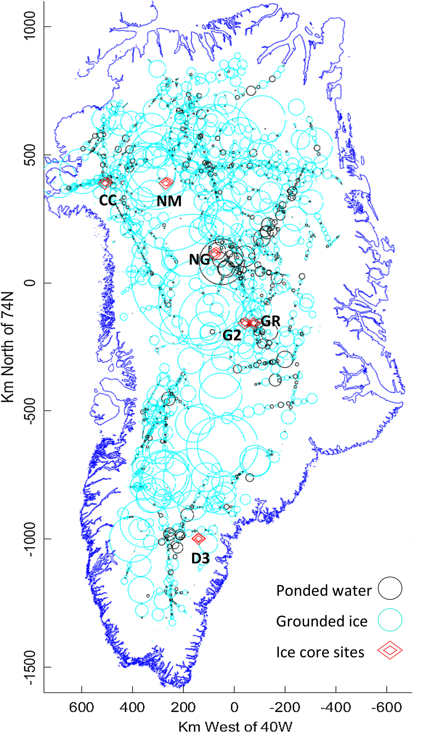
This scale of effective continuity along the survey flight is then used to extrapolate the effectively continuous condition over a circular area, based on the thawed segment as diameter, and termed a ‘continuity zone’. In the absence of ponding, the bed is assumed to be grounded (but may in fact be at the pressure melting point) and similar continuity zones are established. In Figure 12, the effective continuity along the flight paths is illustrated in terms of these zones. The grounded and ponded continuity zones are frequently clustered and overlapping, and provide an opportunity for checking consistency between measurements from different flight paths. This check can be applied to nearby flights from different years and different days, or on the same day, as well as flights that overfly nearly the same ground track. Following this procedure, we find that the main features in the map, and the broad form of the distribution, show substantial consistency within and between flights.
Circles of effective continuity of ponded or grounded bed.
This interpolation approach is based on the aspects of the radar signal itself rather than any detailed analysis of the glaciological and topographical context, so that the radar evidence, which is the subject of this paper, can be considered on its own merits.
4.3. Mapping the distribution of ponded subglacial water
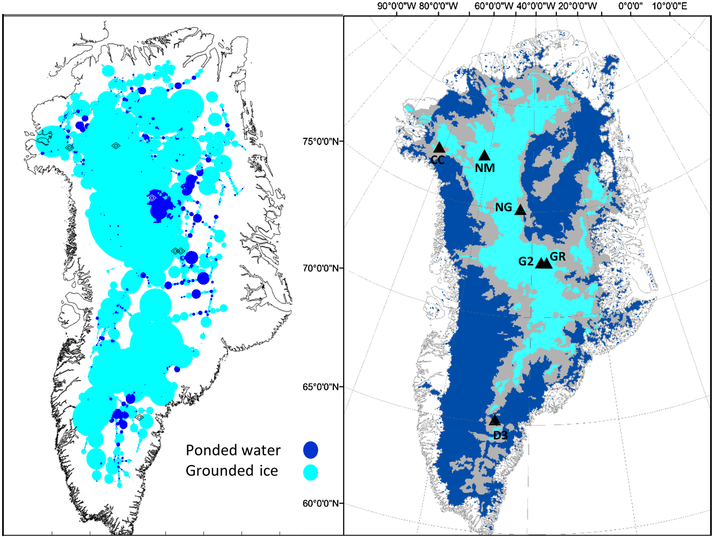
In Figure 13, we present a 1 km rectangular northing/easting grid where the position (0,0) is located at 74N, 40W. The determination at each location is derived from its proximity to the effectively continuous measurements along neighbouring flight paths of the survey (hence the circular plot features in Fig. 12). Figure 13 depicts the resulting map, and provides a determination of the presence of ponded water over a large portion of the ice sheet.
A 1 km grid map illustrating where the ice sheet bed is found to be ponded or to be grounded.
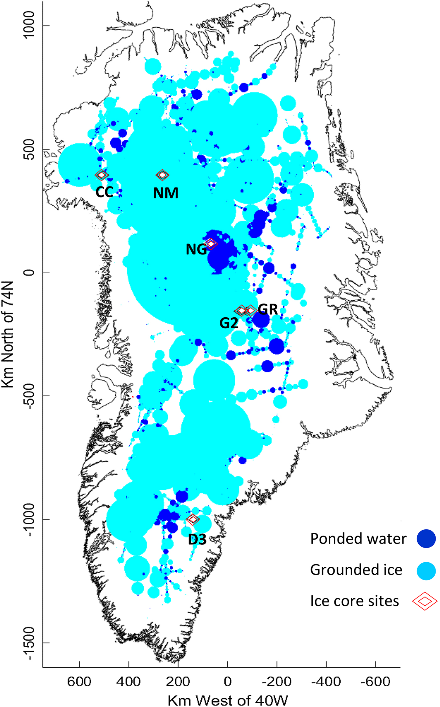
The areas identified as ponded in the far north are reduced in extent compared with Oswald and Gogineni (Reference Oswald and Gogineni2012), and the survey is extended to cover the majority of the Greenland Ice Sheet.
The locations where ponded thaw is identified are stable for a considerable range of threshold values. However, the proportion of the bed that we recognise as ponded thaw is sensitive to the way in which we estimate the continuity of the bed condition. We set a continuity criterion such that separation greater than the ice thickness between determinations of ponding limits the extent of continuity. This leads to a conclusion that the proportion of the bed identified as ponded totals 7.1%.
Zones of basal thaw thick enough for detection by this method are found up to 15 000 km2 in extent, and underlying up to 40 000 km3 of ice. There are several in the 20–80 km scale and increasing numbers at reducing scale. Regions containing multiple interlinked grounded areas are found that extend over more than 200 km. The total volume of ice underlain by ponded areas is estimated at over 140 000 km3.
Because our method detects regions with a relatively thick layer of ponded water, this extent must be smaller than that of all regions with temperate bed. The extent is compared with that of temperate bed predicted by MacGregor and others (Reference MacGregor2016) in Figure 15. In principle, our results must be a subset of the extent of temperate bed. However, discrepancies exist between the two results, and we will explore the distributions in Section 5 below.
4.4. Internal consistency in the results
Results at any point in the 1 km grid include the measured, linearly interpolated and/or laterally inferred basal condition. The internal consistency of these is illustrated by the substantially comparable overlapping circles of continuity shown in Figure 12.
For an effective test of consistency, comparisons are made on the observed scale of thaw features.
These are reported below. In summary, a total of over 1 million points in the 1 km map grid yielded at least one decision on the bed state. Of these, 72 060 yielded a thaw determination, yielding the estimate that 7.1% of the bed lies on ponded thaw.
For a 1 km grid of the Greenland Ice Sheet, a total of 1 016 978 grid squares contain at least one decision on the bed condition. Decisions at each point are based on up to 14 flight transits. Of those grid points, 93% yield a grounded condition and 7% yield a ponded condition. Full consistency is found at over 90% of points; consistency is determined by up to four ‘ponded’ votes or up to 14 grounded votes, with the casting vote for the ‘ponded’ minority. Of the <10% of grid points yielding a mixed decision, over 57% yield a ponded majority, while 43% yield a grounded majority.
For such a large population, this high degree of consistency suggests that decisions were not influenced by flight directions or basal anisotropy, since many different flight directions are represented.
There is one exception to this, at Camp Century. Most flights in the northern region began from Thule Air Force Base and overflew Camp Century before deploying to different survey paths. This means that the area along the flight path between Thule and Camp Century was over-represented in the survey. In addition, these flight segments were closely clustered and were predominantly oriented close to the estimated flow direction of ice (Zwally and Giovinetto, Reference Zwally and Giovinetto2001) and of possible basal erosion. For that reason, we have included only a subset of data from that region.
5. DISCUSSION OF THE DISTRIBUTION OF PONDED THAW
Evidence of subglacial water has been found (Dahl-Jensen and others, Reference Dahl-Jensen, Gundestrup, Gogineni and Miller2003) at the base of the NorthGRIP ice core, and subglacial water is expected in locations such as the bed of the NEGIS. From the radar data, one of the most striking features of the continuity zones and the map of subglacial ponding is an area near and to the northwest of the onset of the NEGIS, with an extended spur stretching north-eastward, close to the line of the NEGIS. The location of this thawed area confirms that the water that is expected at the base of such an ice stream shows up clearly in our analysis of radar data. This result also provides robust a priori information on the basal status of NEGIS that can be used to validate modelling results.
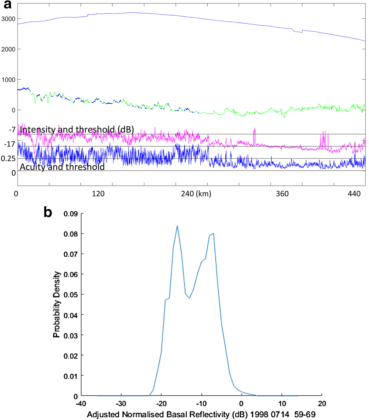
Elsewhere, ponded thaw is detected more persistently beneath the Summit Dome and to the east of the north-south grounded axis in another extensive area of detected ponding to the south of GRIP and GISP 2. This area lies west of the east-central subglacial highlands and provides a strong candidate for investigation of the motion of the overlying ice. This may suggest elevated GHF, and flow mapping (Mouginot and others, Reference Mouginot, Rignot, Scheuchl and Millan2017) suggests that it may affect the flow of Daugaard-Jensen, Vestfjord and Kangerdlugssuaq glaciers. A detailed examination of topography and basal hydrology in this and more recent datasets would be needed to find whether a connection exists. For reference, Figure 14 shows results from a flight segment (‘E’ in Fig. 2), which originates from the flight of 14 July 1998. This segment crosses much of the ice sheet, including this feature, and meets criteria for ponded thaw beneath much of the eastern part of the track. We will revisit this feature using a numerical ice-sheet model in Section 5.1.
(a) Segment E (Fig. 2) profile with intensity and acuity, indicating an extended area of ponded thaw in east central Greenland, with grounded ice to the west. (b) Segment E normalised reflectivity histogram.
A further concentration of thaw ponding is detected beneath the southern dome of the ice sheet near (65N, 45W) in Figures 12, 13. This may feed the onset of Helheim Glacier, but is over 100 km away.
An extensive but scattered area of thaw is also apparent beneath the western slope of the ice sheet and including the area east of Jakobshavns Isbræ where a number of ponded continuity zones of diameter over 20 km are shown. The periphery of this area may be that most affected by the low sensitivity of this method to very thin layers of thaw, in these areas suggesting that although thaw may be widespread, ponding is more scattered.
In the north, basal thaw is detected over a wide area but in smaller pockets that was suggested by the earlier, over-simple model of dielectric attenuation (Oswald and Gogineni, Reference Oswald and Gogineni2012). There are many indications of areas of ponding of scale 10–50 km, but at the scale of the map, and without direct reference to basal topography, there is little clear pattern in their distribution with respect to outflow glaciers. Indeed, the drainage afforded by glaciers may reduce the likelihood of radar detection of basal thaw.
5.1. Comparison with a numerical synthesis
MacGregor and others (Reference MacGregor2016), hereafter referred to as MGR, have estimated basal temperatures in Greenland by a synthesis of thermomechanical modelling, radiostratigraphy, surface ice velocity and texture and borehole observations, and we here refer to this study as an initial check on the link between radar observations and other glaciological methods.
As described above, in this study, detection thresholds have been set at values appropriate to identify water layers at least 3 cm thick. A bed region at the pressure melting point may therefore not be detected by radar if the melt rate is low or the topography allows meltwater to drain. To be consistent, the results from radar need not match, but should fall within the regions that are identified as temperate bed by MGR. The MGR results indeed predict more widely distributed basal thaw than the derived ponding that is detected and inferred by radar. This comparison is illustrated in Figure 15.
Broad comparison of regions with observed (left panel, this study), and modelled (right panel, from MacGregor and others, Reference MacGregor2016) bed conditions. Cyan regions in the left panel represent the absence of ponded water but not necessarily a frozen bed. These projections are not identical, but indicate areas of broad correspondence or anomaly between the model and the radar evidence.
The region of greatest consistency is the onset location of NEGIS, where radar echograms (Fahnestock and others, Reference Fahnestock, Abdalati, Joughin, Brozena and Gogineni2001), modelling studies (e.g. Rogozhina and others, Reference Rogozhina2016) and geophysical surveys (Christianson and others, Reference Christianson2014) suggest a region of potentially high heat flux and basal thaw. In the region beneath the northerly reaches of the NEGIS, ponding appears to have subsided in the interpolated radar data, but features are present among the continuity zones. Here it is reasonable that basal thaw in fact occurs but drainage keeps the water layer too thin to detect. It is also possible that the distribution of flight paths combined with the method of interpolation obscures the continuity of radar signals.
The majority of the coastal regions where we find pockets of isolated ponded water also correspond well in terms of location with MGR results, most notably in the central-west region upstream of Jakobshavns Isbræ, although continuity is limited.
In south Greenland, we find significant pockets of ponded water to the north and west of Dye-3, but not covering the ice core site (with measured −13°C basal temperature). Except near the ice divides of the south, MGR also predict thawed bed in southern Greenland which corresponds well with our results. However, Rezvanbehbahani (in preparation) has shown that the expected geological structure in this area implies low values of GHF and might require high-GHF rock intrusions to match this pattern of thaw.
A region of mismatch occurs at the NorthGRIP site. This location is within a region identified by radar on multiple flights as ponded, and found to be actually thawed at the base of the ice core (Dahl-Jensen and others, Reference Dahl-Jensen, Gundestrup, Gogineni and Miller2003). According to the MGR results, this ice core site lies outside several modelled thaw predictions.
The sharpest contrast between our results and MGR is the area centred near 71oN, 38oW, with a radius of ~100 km, south and east of the GRIP and GISP 2 ice core sites. Here the evidence for areas of ponding appears strong in the radar data, and is repeated in different years and neighbouring flights, while nearly all the numerical models used in MGR predict a majority of frozen and therefore grounded bed in this region (MacGregor and others, Reference MacGregor2016, Figure 4). However, all those models also apply the seismically inferred GHF (Shapiro and Ritzwoller, Reference Shapiro and Ritzwoller2004, with minor adjustments) as a boundary condition and, therefore, their consensus is not surprising. In the next section, we briefly investigate whether this discrepancy can be justified in terms of possible spatial variability of GHF. The detailed investigation is a topic of another study by Rezvanbehbahani and others (in preparation).
5.2. Implications of ponded thaw detection for model boundary conditions
Although the basal thermal state (frozen vs thawed) does not appear as a direct boundary condition in ice-sheet models, determination of the basal condition as between ponded or grounded carries significant information about these boundary conditions. At basal locations that are thawed and ponded, based on an ice-sheet model, the maximum GHF can be obtained above which the bed will become thawed. Here, we provide the preliminary results of such implications of the data presented in this study.
Assuming that the distribution of basal thaw is primarily due to variations of the GHF, we iteratively adjust the values of GHF in a numerical ice-sheet model SICOPOLIS (similar to Greve, Reference Greve2005) so that the melt rates at radar-detected thawed regions become positive but <10 mm year−1 (i.e. close to the melting point). The results of these iterations for regions with surface elevation above 2000 m.a.s.l. are shown in Figures 16a, b.
The minimum GHF required to thaw the bed in central east Greenland (Fig. 16a) shows moderate-to-elevated GHF values, while the value found at the GRIP ice core site was 51.4 mW m−2 (Dahl-Jensen and others, Reference Dahl-Jensen1998). The moderate values of GHF (~50–60 mW m−2) do not provide additional information or constraints about the underlying bedrock.
Results of adjusting the GHF using SICOPOLIS at locations of basal thaw in central east Greenland obtained from radar data (this study). The adjusted GHF, panel (a), shows the minimum GHF required to thaw the bed, and panel (b) shows the corresponding melt rate. Ice core locations are shown with blue triangles. For details of the adjustment procedure refer to Rezvanbehbahani and others (in preparation).
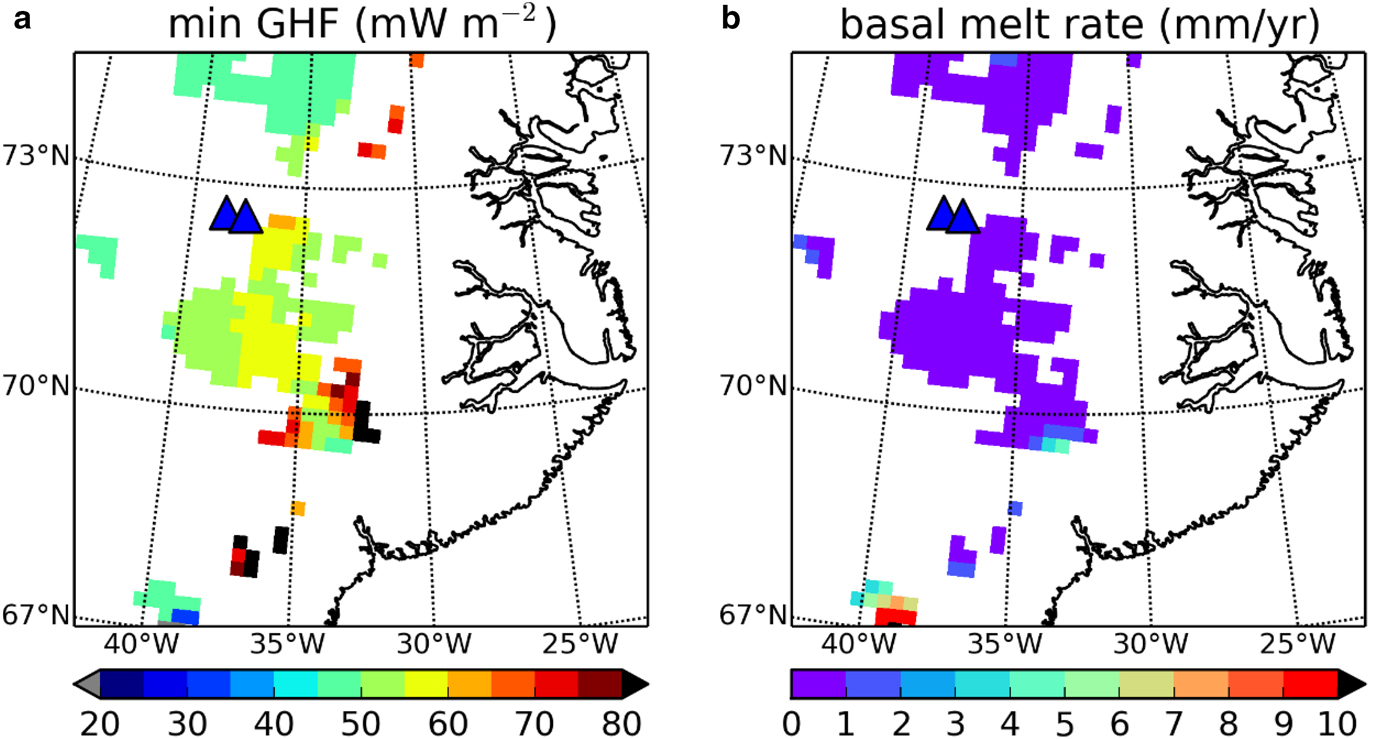
At other pockets of thaw in this region, minimum GHF appears to be 60–90 mW m−2. This is higher than the continental background and implies a locally elevated GHF in this region. Similar high-GHF features are illustrated by Fox Maule and others (Reference Fox Maule, Purucker and Olsen2009), centred near 70N, 30W (~360 km N, −440 km W in the XY reference frame). The high GHF from seismically inferred maps (Shapiro and Ritzwoller, Reference Shapiro and Ritzwoller2004) is positioned further to the southeast of our predicted basal thaw (refer to Rogozhina and others, Reference Rogozhina2012 for comparison of different GHF maps). Our estimates of high GHF values and the strong radar indication of basal thaw both in this region and in the south of the ice sheet are suggestive about the geologic properties, possibly due to features such as dykes in the bedrock. Therefore, we suggest that these regions merit further investigation.
6. CONCLUSIONS
We describe the extent of subglacial ponded water beneath substantial portions of the ice sheet, using a radar analysis that is similar to but calculated in finer detail than the earlier descriptions of this technique (Oswald and Gogineni, Reference Oswald and Gogineni2012). These results show consistency with ground truth data, including at NorthGRIP and at Camp Century in northern Greenland. We show widespread ponded thaw beneath ~7% of the Greenland Ice Sheet. This total area is less than that of pressure melting suggested by combined numerical ice-sheet models and radiostratigraphy (MacGregor and others, Reference MacGregor2016); however, this analysis of radar signals is sensitive only to significantly ponded water intrusions; that is, areas where the water depth is >~3 cm. A key point of confirmation is that extensive thaw is found beneath the NEGIS and its tributary area beneath the spine of the ice sheet, and extending around the NorthGRIP core-drilling site, where basal water was found.
The great majority of the identified basal water takes the form of a layer between ice and rock that apparently conforms to but smooths, on the scale of metres, the small-scale bedrock topography, forming ‘ponds’ rather than extensive, specularly smooth ‘lakes’ as have been identified in Antarctica.
We have shown that radar allows us to measure distinct geometric and material aspects of the subglacial interface, allowing the more highly reflective, smoother segments to be resolved and identified, and we have shown that the radar signal characteristics are associated with the nature of the bed itself rather than with uncertainties in the propagation through the ice column.
By associating the radar results with numerical models of the ice sheet, we have identified an area south of GRIP and GISP 2, on a scale of 200 km diameter, within which ponding is evident but unexpected. There the GHF may somewhat exceed the continental background, in substantial agreement with the magnetically inferred model of the GHF (Fox Maule and others, Reference Fox Maule, Purucker and Olsen2009), and with significance for boundary conditions in thermo-mechanical models of the ice sheet.
We have also been able to provide maps of the mean absorption rate of the radar signal in propagation through the ice, and shown that its SD is small compared with the measured values.
Our results are used in another study by Rezvanbehbahani and others (in preparation) to constrain the GHF models for Greenland and aid prediction of the behaviour of the ice sheet. They allow a lower limit of GHF to be placed on apparently thawed interior regions of the ice-sheet bed, thereby increasing the significance of the model results, providing a large set of relevant test data and opening the way to increasing the robustness of predictions of the state of the Greenland Ice Sheet.
This investigation could be extended to a detailed analysis of the bed topography together with the bed state, to determine the likely connectivity of basal water sources and flows, especially as new survey programmes deliver increased and more detailed coverage of the ice sheet.
ACKNOWLEDGEMENTS
This work has been supported under NSF ARRA Grant 0909431, and by the University of Maine Climate Change Institute. S.R. and L.A.S. were supported by the Center for Remote Sensing of Ice Sheets at the University of Kansas. We are grateful for this support, and also for the feedback and encouragement of Roger Le B Hooke, Paul Mayewski and Kees van der Veen at these institutions. We also thank Joseph MacGregor for providing the data of his prediction of basal thermal state.


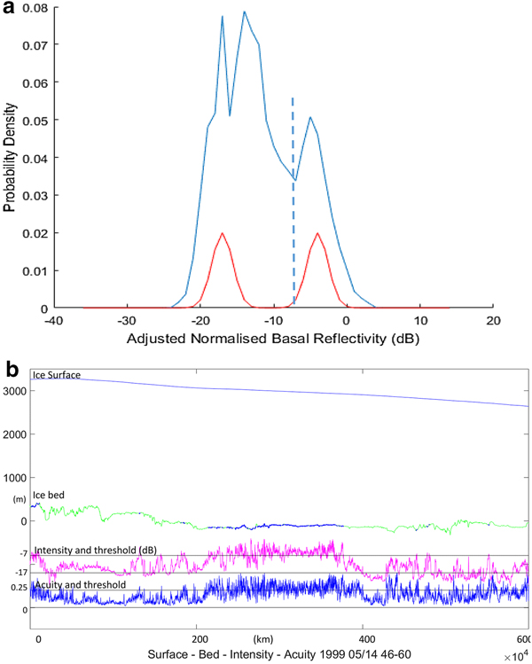


 Open access