


1 Introduction
Latent variable models are widely used in psychometrics to explain the covariance between a set of observed variables by a set of unobserved, or latent variables. The most common way to fit latent variable models is by marginal maximum likelihood (MML) using the expectation–maximization (EM) algorithm, which is attractive due to its asymptotic properties. However, when the number of latent dimensions in the model increases, MML can become computationally infeasible due to the high-dimensional nature of the integral in the marginal likelihood. This computational burden is further amplified by larger sample sizes, which increase the amount of data over which these integrals have to be evaluated. Yet, large, high-dimensional datasets are becoming more and more common due to the ease of online data collection, the rise of educational and psychological monitoring systems, and the increased availability of process data. Various solutions to this computational problem exist in the literature, such as adaptive quadrature (Bock & Aitkin, Reference Bock and Aitkin1981), Markov chain Monte Carlo (MCMC) (Edwards, Reference Edwards2010), stochastic approximation (Cai, Reference Cai2010; von Davier & Sinharay, Reference von Davier and Sinharay2010), and joint maximum likelihood (Chen et al., Reference Chen, Li and Zhang2019). However, fitting high-dimensional models to large datasets is generally still computationally challenging.
An alternative to MML that has recently been developed to estimate latent variable models is standard variational inference (VI). These methods approximate the posterior distribution of the latent variables by a highly factorial distribution. By sampling from this approximate distribution, a lower bound on the marginal likelihood can be maximized to obtain parameter estimates (Blei et al., Reference Blei, Kucukelbir and McAuliffe2017). This method was originally developed in a Bayesian context and has been used to estimate Bayesian item response theory (IRT) (Wu et al., Reference Wu, Davis, Domingue, Piech and Goodman2021) and cognitive diagnostic (Yamaguchi & Okada, Reference Yamaguchi and Okada2020) models successfully. However, the same approach has also been used to estimate models with fixed item parameters (Cho et al., Reference Cho, Wang, Zhang and Xu2021). Furthermore, by taking multiple samples from the approximate posterior using importance-weighted sampling (Kahn & Marshall, Reference Kahn and Marshall1953), the lower bound can be made arbitrarily close to the marginal likelihood depending on the number of samples, approaching the MML solution (Ma et al., Reference Ma, Ouyang, Wang and Xu2023).
Although VI avoids the evaluation of the integral in the marginal likelihood, the posterior parameters for each individual must be estimated. The number of variational parameters scales with the sample size N, which becomes computationally intensive for large datasets and high-dimensional models, especially if there is no closed-form update possible for the approximate posteriors. This drawback is avoided in amortized VI (AVI), where instead of directly optimizing the posterior parameters, a so-called inference model is estimated. This inference model relates the observed data to the posterior parameters using some non-linear parametric function. That is, the posterior parameters are amortized. Note that this is different from Bayesflow style amortization (Radev et al., Reference Radev, Mertens, Voss, Ardizzone and Köthe2020), which relies on large-scale simulation to train a network that maps data to posterior distributions. In AVI, amortization refers only to predicting parameters of the approximate posteriors from the observed data, not relying on any simulation. During estimation, the parameters of the approximate posterior are computed using the current estimates from the inference model, a sample is taken from the approximate posterior, and the parameters of the measurement and inference models are updated jointly using gradient descent. The use of amortization improves the estimation efficiency on large datasets and high-dimensional models as the number of parameters in the inference model depend on the number of items but not on the number of individuals. Curi et al. (Reference Curi, Converse, Hajewski and Oliveira2019) were one of the first to use such an approach to estimate IRT parameters, and Urban and Bauer (Reference Urban and Bauer2021) extended this approach to include multiple importance-weighted samples from the approximate posterior to approximate the marginal likelihood solution even closer. In both studies, it is demonstrated that for large, high-dimensional data, this method of estimation is much faster than state-of-the-art MML implementations, while still attaining approximately equally accurate parameter estimates. Since then, the AVI approach has been applied to a broad range of IRT models. For example, the approach has been generalized to the three- and four-parameter logistic IRT models (Liu et al., Reference Liu, Wang and Xu2022), models that allow for correlated latent variables (Converse et al., Reference Converse, Curi, Oliveira and Templin2021), fixed effect IRT models (Molenaar et al., Reference Molenaar, Grasman and Cúri2025), models that jointly model responses and response times (Debelak & Urban, Reference Debelak and Urban2021), and models that amortize over both person and item parameters (Zhang & Chen, Reference Zhang and Chen2024). Additionally, the model has been generalized to situations where the factor loading structure is misspecified (Hasan et al., Reference Hasan, Deng, Sabatini, Bowman, Yang and Hollander2022) and to models for data with a significant proportion of missingness (Veldkamp et al., Reference Veldkamp, Grasman and Molenaar2024).
When looking at the taxonomy of latent variable models by Bartholomew et al. (Reference Bartholomew, Knott and Moustaki2011) in Table 1, it is interesting to note that currently, the applications of AVI mostly—if not exclusively—focus on IRT models. Although it is straightforward to generalize the AVI approach to factor analysis, the benefits are less prominent as there is a closed-form solution for the integrals in the marginal likelihood of the (normal theory) linear factor model. A more interesting application for AVI concerns models with discrete latent variables, such as latent class and latent profile models. Such discrete latent variable models have many important applications in the fields of educational psychology (de la Torre & Minchen, Reference de la Torre and Minchen2014), clinical psychology (Sullivan et al., Reference Sullivan, Kessler and Kendler1998), medicine (Formann & Kohlmann, Reference Formann and Kohlmann1996), and sociology (Yamaguchi, Reference Yamaguchi2000). Although there is no closed-form solution for the integrals in the marginal likelihood of latent variable models including latent classes, the computational advantage of AVI for simple latent class or latent profile models is expected to be limited. That is, evaluating the integrals in the marginal likelihood of a discrete latent variable model is computationally less demanding as the parameter space to be intergrated over is much smaller than that of the continuous latent variables in IRT models.
Four types of latent variable models according to the taxonomy of Bartholomew et al. (Reference Bartholomew, Knott and Moustaki2011)

Although AVI has not been used for discrete latent variables, standard VI has successfully been used to estimate discrete latent variable models. For example, Grimmer (Reference Grimmer2011) used VI to estimate latent class models and Oka and Okada (Reference Oka and Okada2023) and Yamaguchi and Okada (Reference Yamaguchi and Okada2020) used VI to estimate cognitive diagnostic models. These papers are both fully Bayesian including prior on both the latent variables and the item parameters. However, priors on the item parameters are by no means a requirement for a discrete VI approach, and we estimate fixed item parameters in this work. Importantly, previous work on VI and discrete latent variables use conjugate priors, yielding closed-form analytical updates for the variational posteriors, greatly improving estimation efficiency. However, as the conditional distributions involved need to be part of the exponential family, the generalizability of these approaches is relatively limited.
Hybrid models that include both discrete and continuous latent variables, such as mixture IRT models (Sen & Cohen, Reference Sen and Cohen2019) and factor mixture models (Kim et al., Reference Kim, Wang and Hsu2023), can therefore potentially benefit substantially from AVI, particularly when the observed variables are categorical. In such models, both the discrete and continuous latent variables need to be integrated out of the likelihood, so estimation becomes computationally challenging even with a moderate number of latent variables. Extending the AVI framework to these hybrid models, while avoiding restrictive conjugacy assumptions, is thus a promising direction. However, as discussed below, incorporating discrete latent variables into AVI is not straightforward.
Estimating the parameters of the inference model requires reparameterizing the sampling process into a differentiable function that depends on the parameters from the posterior distribution and a random variable with fixed parameters (Kingma & Welling, Reference Kingma and Welling2013). While this is straightforward for continuously distributed latent variables, it is more challenging for discrete latent variables (see Section 3 for a detailed discussion). Several techniques have been proposed in the machine learning literature that allow sampling from discrete distributions. However, while machine learning applications focus on predictive accuracy, latent variable modeling is primarily concerned with accurate parameter estimates, since the parameters themselves carry substantive meaning and are used for (high-stakes) practical decisions. In the current article, we propose two methods to incorporate discrete latent variables in the AVI framework. We provide a systematic comparison of these methods in estimating latent class models and cognitive diagnostic models. Then, we demonstrate how the most promising method can be generalized to more complex, hybrid latent variable models such as a multidimensional mixture latent variable model, and demonstrate its computational advantage.
The outline is as follows: First, we formally introduce AVI and discuss the challenges related to discrete latent variables. Next, we propose two solutions. We evaluate these solutions in a preliminary simulation devoted to latent class analysis (LCA) and generalized deterministic inputs, noisy and gate (GDINA) models, verifying that AVI can be used for discrete latent variables. In our main simulation study, we apply the methods for discrete latent variables to estimate a mixture multidimensional IRT model, and demonstrate its computational advantage compared to MML. We then apply this mixture IRT method to a real seven-dimensional large-scale dataset pertaining to Narcissism. We end with a general discussion.
2 Amortized variational inference
Consider a general latent variable model in which the latent variable vector is denoted by $\boldsymbol {\theta } \in \mathbb {R}^d$
and the corresponding observed response vector is denoted by
$\boldsymbol {\theta } \in \mathbb {R}^d$
and the corresponding observed response vector is denoted by $\mathbf {x}$
. Note that
$\mathbf {x}$
. Note that $\boldsymbol {\theta }$
may be continuous or categorical depending on the type of model. The domain will always be clear from the context. The joint distribution of
$\boldsymbol {\theta }$
may be continuous or categorical depending on the type of model. The domain will always be clear from the context. The joint distribution of $\boldsymbol {\theta }$
and
$\boldsymbol {\theta }$
and $\mathbf {x}$
can be written as
$\mathbf {x}$
can be written as
 $$ \begin{align} p_\psi(\boldsymbol{\theta}, \mathbf{x}) = p_\psi(\mathbf{x} \mid \boldsymbol{\theta})\, p(\boldsymbol{\theta}), \end{align} $$
where $p_\psi (\mathbf {x} \mid \boldsymbol {\theta })$
represents the likelihood or measurement model parameterized by (fixed effects) parameters
$p_\psi (\mathbf {x} \mid \boldsymbol {\theta })$
represents the likelihood or measurement model parameterized by (fixed effects) parameters $\psi $
, and
$\psi $
, and $p(\boldsymbol {\theta })$
denotes the population distribution of the (random effects) latent variables. The corresponding posterior distribution of the latent variables given the observed responses is then
$p(\boldsymbol {\theta })$
denotes the population distribution of the (random effects) latent variables. The corresponding posterior distribution of the latent variables given the observed responses is then
 $$ \begin{align} p_\psi(\boldsymbol{\theta} \mid \mathbf{x}) = \frac{p_\psi(\mathbf{x} \mid \boldsymbol{\theta})\, p(\boldsymbol{\theta})} {p_\psi(\mathbf{x})}, \end{align} $$
where $p_\psi (\mathbf {x}) = \mathbb {E}_{p(\boldsymbol {\theta })}[\, p_\psi (\mathbf {x}\mid \boldsymbol {\theta })]$
is the marginal likelihood. Each individual i has their own latent variable vector
$p_\psi (\mathbf {x}) = \mathbb {E}_{p(\boldsymbol {\theta })}[\, p_\psi (\mathbf {x}\mid \boldsymbol {\theta })]$
is the marginal likelihood. Each individual i has their own latent variable vector $\boldsymbol {\theta }_i$
and posterior
$\boldsymbol {\theta }_i$
and posterior $p_\psi (\boldsymbol {\theta }_i | \mathbf {x}_i)$
, but for notational clarity, we drop the index i and write all expressions for a generic observation
$p_\psi (\boldsymbol {\theta }_i | \mathbf {x}_i)$
, but for notational clarity, we drop the index i and write all expressions for a generic observation $(\mathbf {x}, \boldsymbol {\theta }).$
In latent variable models for categorical data, this posterior can be computationally expensive to compute or even intractable in the case of continuous latent variables, motivating the use of VI methods.
$(\mathbf {x}, \boldsymbol {\theta }).$
In latent variable models for categorical data, this posterior can be computationally expensive to compute or even intractable in the case of continuous latent variables, motivating the use of VI methods.
As already mentioned above, in standard VI, the true posterior distribution is approximated by an approximate posterior distribution which typically (but not necessarily) is a factorized normal distribution. We denote this variational approximation by $q(\boldsymbol {\theta } \mid \mathbf {x})$
, meaning the approximate posterior over the latent variable vector
$q(\boldsymbol {\theta } \mid \mathbf {x})$
, meaning the approximate posterior over the latent variable vector $\boldsymbol {\theta } \in \mathbb {R}^d$
given the response vector
$\boldsymbol {\theta } \in \mathbb {R}^d$
given the response vector $\mathbf {x}$
. The idea behind VI is to choose the approximate posterior
$\mathbf {x}$
. The idea behind VI is to choose the approximate posterior $\hat q \in \mathcal {F}$
so that the Kullback–Leibler (KL) divergence to the true posterior,
$\hat q \in \mathcal {F}$
so that the Kullback–Leibler (KL) divergence to the true posterior, $p_\psi (\boldsymbol {\theta } \mid \mathbf {x})$
, is minimized:
$p_\psi (\boldsymbol {\theta } \mid \mathbf {x})$
, is minimized:
 $$ \begin{align} \hat{q}(\boldsymbol{\theta} \mid \mathbf{x}) = \operatorname*{\mathrm{argmin}}_{q(\boldsymbol{\theta} \vert \mathbf{x}) \in \mathcal{F}} \text{KL}[q(\boldsymbol{\theta} \mid \mathbf{x}) \mid \mid p_{\psi}(\boldsymbol{\theta} \mid \mathbf{x})]. \end{align} $$
Here, $\mathcal F$
is a chosen family of allowed approximate posterior distributions. The family
$\mathcal F$
is a chosen family of allowed approximate posterior distributions. The family $\mathcal F$
is usually restricted; for example, to a highly factorized family of distributions. It can be shown that minimizing the KL divergence between the approximate posterior distribution and the trution (Equation (3)) can be accomplished indirectly by maximizing the so-called evidence lower bound (ELBO)
$\mathcal F$
is usually restricted; for example, to a highly factorized family of distributions. It can be shown that minimizing the KL divergence between the approximate posterior distribution and the trution (Equation (3)) can be accomplished indirectly by maximizing the so-called evidence lower bound (ELBO)
 $$ \begin{align} \text{ELBO}={{\mathbb{E}}}_{q(\boldsymbol{\theta} \mid \mathbf{x})}[\log p_{\psi}(\mathbf{x} \mid {\boldsymbol{\theta}})] - \text{KL}[q(\boldsymbol{\theta} \mid \mathbf{x}) \mid \mid p(\boldsymbol{\theta})], \end{align} $$
where $p(\boldsymbol {\theta })$
is the prior distribution evaluated at
$p(\boldsymbol {\theta })$
is the prior distribution evaluated at $\boldsymbol {\theta }$
(Blei et al., Reference Blei, Kucukelbir and McAuliffe2017). The ELBO gives a lower bound to the marginal log-likelihood. It approaches the marginal log-likelihood when the approximate posterior distribution approaches the true posterior distribution. In VI, item parameters
$\boldsymbol {\theta }$
(Blei et al., Reference Blei, Kucukelbir and McAuliffe2017). The ELBO gives a lower bound to the marginal log-likelihood. It approaches the marginal log-likelihood when the approximate posterior distribution approaches the true posterior distribution. In VI, item parameters $\psi $
are estimated by maximizing this ELBO.
$\psi $
are estimated by maximizing this ELBO.
As discussed above, to avoid estimating separate approximate posterior $\hat {q}$
for each individual, in AVI a general, shared inference model
$\hat {q}$
for each individual, in AVI a general, shared inference model $q_\zeta $
with parameters
$q_\zeta $
with parameters $\zeta $
is introduced which maps each individual response pattern to its approximate posterior distribution. In other words, instead of optimizing a new variational estimate
$\zeta $
is introduced which maps each individual response pattern to its approximate posterior distribution. In other words, instead of optimizing a new variational estimate $\hat {q}$
for every individual, we estimate a single function that models the relation between the approximate posterior parameters and the observed data. Formally, we choose
$\hat {q}$
for every individual, we estimate a single function that models the relation between the approximate posterior parameters and the observed data. Formally, we choose
 $$ \begin{align} \boldsymbol{\theta}\mid \mathbf{x} \sim q_\zeta(\boldsymbol{\theta}\mid \mathbf{x}), \end{align} $$
where $q_\zeta $
is an inference model with parameters
$q_\zeta $
is an inference model with parameters $\zeta $
. As such, the approximate posterior is parameterized using parameters
$\zeta $
. As such, the approximate posterior is parameterized using parameters $\zeta $
common to all individuals. The number of parameters does not depend on the number of individuals. When both the inference model and the measurement model are neural networks, this architecture is also known as a variational autoencoder (VAE) (Kingma & Welling, Reference Kingma and Welling2013).
$\zeta $
common to all individuals. The number of parameters does not depend on the number of individuals. When both the inference model and the measurement model are neural networks, this architecture is also known as a variational autoencoder (VAE) (Kingma & Welling, Reference Kingma and Welling2013).
Although the ELBO is indeed a lower bound to the marginal log-likelihood regardless of the choice of the posterior distribution $q_\zeta (\boldsymbol {\theta }\mid \mathbf {x})$
, one often assumes an overly simplified, highly factorized form of
$q_\zeta (\boldsymbol {\theta }\mid \mathbf {x})$
, one often assumes an overly simplified, highly factorized form of $q_\zeta (\boldsymbol {\theta }\mid \mathbf {x})$
. Burda et al. (Reference Burda, Grosse and Salakhutdinov2015) show that this assumption of a simple factorized posterior distribution can lead to a large gap between the ELBO and the marginal likelihood. In order to solve this issue, they propose to use importance-weighted sampling using the approximate posterior distribution as proposal distribution and the joint distribution
$q_\zeta (\boldsymbol {\theta }\mid \mathbf {x})$
. Burda et al. (Reference Burda, Grosse and Salakhutdinov2015) show that this assumption of a simple factorized posterior distribution can lead to a large gap between the ELBO and the marginal likelihood. In order to solve this issue, they propose to use importance-weighted sampling using the approximate posterior distribution as proposal distribution and the joint distribution $p_\psi (\boldsymbol {\theta }, \mathbf {x})$
as target distribution. This results in the importance-weighted ELBO (IW-ELBO)
$p_\psi (\boldsymbol {\theta }, \mathbf {x})$
as target distribution. This results in the importance-weighted ELBO (IW-ELBO)
 $$ \begin{align} \text{IW-ELBO} = \mathbb{E}_{1:S} \left[ \log \frac{1}{S}\sum_{s=1}^S\frac{p_\psi( \tilde{\boldsymbol{\theta}}^{(s)},\mathbf{x})}{q_\zeta(\tilde{\boldsymbol{\theta}}^{(s)}\mid\mathbf{x})}\right], \end{align} $$
where S is the number of importance-weighted samples, and $\tilde {\boldsymbol {\theta }}^{(s)} \sim q_\zeta (\boldsymbol {\theta } \mid \mathbf {x})$
are samples drawn from the approximate posterior distribution. By taking the expectation of the joint likelihood using importance-weighted sampling, the IW-ELBO approximates the marginal likelihood more closely. In fact, Burda et al. prove that, as S increases, the IW-ELBO approaches the marginal log-likelihood. Since increasing the number of importance weights can decrease the signal-to-noise ratio of the inference model gradients (Rainforth et al., Reference Rainforth, Kosiorek, Le, Maddison, Igl, Wood and Teh2018), it is generally preferable to use doubly reparameterized gradients (DReG), which provide a low-variance unbiased estimate of the IW-ELBO gradients for importance-weighted AVI (Tucker et al., Reference Tucker, Lawson, Gu and Maddison2018). Urban and Bauer (Reference Urban and Bauer2021) applied IW-AVI to the estimation of high-dimensional IRT models and showed that taking multiple importance-weighted samples results in parameter estimates that are on par with MML estimates, while these estimates are obtained much more efficiently.
$\tilde {\boldsymbol {\theta }}^{(s)} \sim q_\zeta (\boldsymbol {\theta } \mid \mathbf {x})$
are samples drawn from the approximate posterior distribution. By taking the expectation of the joint likelihood using importance-weighted sampling, the IW-ELBO approximates the marginal likelihood more closely. In fact, Burda et al. prove that, as S increases, the IW-ELBO approaches the marginal log-likelihood. Since increasing the number of importance weights can decrease the signal-to-noise ratio of the inference model gradients (Rainforth et al., Reference Rainforth, Kosiorek, Le, Maddison, Igl, Wood and Teh2018), it is generally preferable to use doubly reparameterized gradients (DReG), which provide a low-variance unbiased estimate of the IW-ELBO gradients for importance-weighted AVI (Tucker et al., Reference Tucker, Lawson, Gu and Maddison2018). Urban and Bauer (Reference Urban and Bauer2021) applied IW-AVI to the estimation of high-dimensional IRT models and showed that taking multiple importance-weighted samples results in parameter estimates that are on par with MML estimates, while these estimates are obtained much more efficiently.
In these AVI approaches, the parameters of the measurement and inference models are optimized jointly using gradient descent. For notational convenience, we rewrite the ELBO in Equation (4) as $\text {ELBO} = {{\mathbb {E}}}_{q(\boldsymbol {\theta } \mid \mathbf {x})}[f_{\psi }(\boldsymbol {\theta , \mathbf {x}})]$
, where
$\text {ELBO} = {{\mathbb {E}}}_{q(\boldsymbol {\theta } \mid \mathbf {x})}[f_{\psi }(\boldsymbol {\theta , \mathbf {x}})]$
, where $f_{\psi }(\boldsymbol {\theta , \mathbf {x}})$
represents the term inside the expectation operator in the ELBO.
$f_{\psi }(\boldsymbol {\theta , \mathbf {x}})$
represents the term inside the expectation operator in the ELBO.
Deriving an estimate for the gradients with respect to the parameters of the measurement model $\psi $
is straightforward. Since the expectation is taken over a distribution that is not parameterized by
$\psi $
is straightforward. Since the expectation is taken over a distribution that is not parameterized by $\psi $
, we can move the gradient inside the expectation:
$\psi $
, we can move the gradient inside the expectation:
 $$ \begin{align} \boldsymbol{\nabla}_\psi \text{ELBO} = \nabla_\psi\mathbb{E}_{q_\zeta(\boldsymbol{\theta}\mid\mathbf{x})}[ f_\psi(\boldsymbol{\theta}, \mathbf{x})] = \mathbb{E}_{q_\zeta(\boldsymbol{\theta}\mid\mathbf{x})} [\nabla_\psi f_\psi(\boldsymbol{\theta}, \mathbf{x})], \end{align} $$
and use L Monte-Carlo samples to approximate the expectation:
 $$ \begin{align} \approx \frac{1}{L} \sum_{l=1}^{L}\nabla_\psi f_\psi(\tilde{\boldsymbol{\theta}}^{(l)}, \mathbf{x}). \end{align} $$
However, the same is not the case when taking the gradients with respect to $\zeta $
since the expectation is taken over
$\zeta $
since the expectation is taken over $q_\zeta (\boldsymbol {\theta }\mid \mathbf {x})$
, which is parameterized by
$q_\zeta (\boldsymbol {\theta }\mid \mathbf {x})$
, which is parameterized by $\zeta $
, the gradient cannot simply be moved into the expectation
$\zeta $
, the gradient cannot simply be moved into the expectation
 $$ \begin{align} \boldsymbol{\nabla}_\zeta \text{ELBO} = \nabla_\zeta\mathbb{E}_{q_\zeta(\boldsymbol{\theta}\mid\mathbf{x})} [f_\psi(\boldsymbol{\theta}, \mathbf{x})] \neq \mathbb{E}_{q_\zeta(\boldsymbol{\theta}\mid\mathbf{x})} [\nabla_\zeta f_\psi(\boldsymbol{\theta}, \mathbf{x})]. \end{align} $$
Kingma and Welling (Reference Kingma and Welling2013) point out that this issue can be avoided by reparameterizing $q_\zeta (\boldsymbol {\theta }\mid \mathbf {x})$
as
$q_\zeta (\boldsymbol {\theta }\mid \mathbf {x})$
as $p_{\boldsymbol {\epsilon }}(h_\zeta ({\mathbf {x}}, \boldsymbol {\epsilon })),$
where h is a deterministic function and
$p_{\boldsymbol {\epsilon }}(h_\zeta ({\mathbf {x}}, \boldsymbol {\epsilon })),$
where h is a deterministic function and $\boldsymbol {\epsilon }$
is a random sample from a fixed distribution:
$\boldsymbol {\epsilon }$
is a random sample from a fixed distribution:
 $$ \begin{align} \boldsymbol{\nabla}_\zeta \text{ELBO} = \nabla_\zeta\mathbb{E}_{p_{\boldsymbol{\epsilon}}} [f_\psi(h_\zeta({\mathbf{x}}, \boldsymbol{\epsilon}), \mathbf{x})] = \mathbb{E}_{p_{\boldsymbol{\epsilon}}}[\nabla_\zeta f_\psi(h_\zeta({\mathbf{x}}, \boldsymbol{\epsilon}), \mathbf{x})]. \end{align} $$
Importantly, there should be an unbiased, low-variance estimate of the gradients of $h_\zeta $
in order to effectively estimate
$h_\zeta $
in order to effectively estimate $\zeta $
using this reparameterization. This has implications for the estimation of models with discrete latent variables, which we discuss below.
$\zeta $
using this reparameterization. This has implications for the estimation of models with discrete latent variables, which we discuss below.
3 AVI for discrete latent variable models
As mentioned above, AVI requires the sample from the posterior latent variable distribution to be parameterized in terms of a differentiable function of its parameters and an independent random variable. Although this is possible for most continuous variables, discrete random variables lack such a differentiable reparameterization (Maddison et al., Reference Maddison, Mnih and Teh2016), making it difficult to use AVI when the latent variables are discrete. Below, we discuss two solutions to this problem.
One solution to this problem is to estimate a continuous vector representation for each class and to estimate a vector of the same dimensions in the inference model. Rather than sampling, the model simply chooses the class that has the vector representation closest to the output of the inference model. More specifically, we introduce a vector of free parameters $\boldsymbol {\eta }_c$
of dimensionality D for each latent class c. We will refer to these vectors as class embeddings. The class embeddings are used as input for the measurement model so that the conditional probabilities are conditional on
$\boldsymbol {\eta }_c$
of dimensionality D for each latent class c. We will refer to these vectors as class embeddings. The class embeddings are used as input for the measurement model so that the conditional probabilities are conditional on $\boldsymbol {\eta }_c$
. The inference model is then defined by the step function
$\boldsymbol {\eta }_c$
. The inference model is then defined by the step function
 $$ \begin{align} q_\zeta(\theta=c|\mathbf{x}) = \begin{cases} 1 & \text{for } c = \underset{c \in \{1,\dots,C\}}{\arg\min}\, \| e_\zeta(\mathbf{x}) - \boldsymbol{\eta}_c \|_2, \\ 0 & \text{otherwise,} \end{cases} \end{align} $$
where $e_{\zeta }(\mathbf {x})$
is the output of the inference model, which is a D-dimensional vector in the same space as
$e_{\zeta }(\mathbf {x})$
is the output of the inference model, which is a D-dimensional vector in the same space as $\boldsymbol \eta _c$
. This is effectively mapping the output of the inference model to the nearest class embedding. Although Equation (11) is non-differentiable, one approach is to use the gradients of the ELBO with respect to the class embeddings and use them as if they are the gradients of the ELBO with respect to the output of the inference model, effectively bypassing the non-differentiable nearest neighbor operation. This is a common approach used to obtain gradients through non-differentiable operations often referred to as straight-through estimators (Bengio et al., Reference Bengio, Léonard and Courville2013). Specifically, we copy the gradients with respect to
$\boldsymbol \eta _c$
. This is effectively mapping the output of the inference model to the nearest class embedding. Although Equation (11) is non-differentiable, one approach is to use the gradients of the ELBO with respect to the class embeddings and use them as if they are the gradients of the ELBO with respect to the output of the inference model, effectively bypassing the non-differentiable nearest neighbor operation. This is a common approach used to obtain gradients through non-differentiable operations often referred to as straight-through estimators (Bengio et al., Reference Bengio, Léonard and Courville2013). Specifically, we copy the gradients with respect to $\boldsymbol {\eta }_{c}$
and use them as estimates for the gradients with respect to
$\boldsymbol {\eta }_{c}$
and use them as estimates for the gradients with respect to $\zeta $
. The idea to jointly estimate embeddings and an inference model that maps the data onto the nearest embedding is based on research by van den Oord et al. (Reference van den Oord, Vinyals and Kavukcuoglu2017), who uses deep VAEs to determine low-dimensional representations for image, video, and speech generation. We can use a similar embedding architecture to estimate latent class models. We will refer to the resulting model as the embedding-based latent variable model (ELVM). Note that while ELVM is well suited for latent class analysis, it is not easy to generalize to more complex models, such as cognitive diagnostic models or mixture models. This is because the class-embedding approach represents each class through an unconstrained continuous vector with no direct interpretability. This works well for latent class models because any unconstrained vector can easily be transformed to probabilities (e.g., a neural network). However for cognitive diagnostic models or mixture models, the probabilities must follow from specific predefined algebraic relationship between the parameters, satisfying the mathematical structure of the model. Mapping unconstrained continuous embeddings to such structured parameter spaces is not straightforward.
$\zeta $
. The idea to jointly estimate embeddings and an inference model that maps the data onto the nearest embedding is based on research by van den Oord et al. (Reference van den Oord, Vinyals and Kavukcuoglu2017), who uses deep VAEs to determine low-dimensional representations for image, video, and speech generation. We can use a similar embedding architecture to estimate latent class models. We will refer to the resulting model as the embedding-based latent variable model (ELVM). Note that while ELVM is well suited for latent class analysis, it is not easy to generalize to more complex models, such as cognitive diagnostic models or mixture models. This is because the class-embedding approach represents each class through an unconstrained continuous vector with no direct interpretability. This works well for latent class models because any unconstrained vector can easily be transformed to probabilities (e.g., a neural network). However for cognitive diagnostic models or mixture models, the probabilities must follow from specific predefined algebraic relationship between the parameters, satisfying the mathematical structure of the model. Mapping unconstrained continuous embeddings to such structured parameter spaces is not straightforward.
A second approach to the lack of a differentiable parameterization for the posterior of discrete latent variables is to use a continuous relaxation of the discrete distribution. This substitution enables gradient-based optimization, as the continuous formulation allows derivatives to be computed with respect to model parameters. By selecting a relaxation that includes a tunable temperature or smoothness parameter, one can control the extent to which the continuous approximation resembles a discrete distribution, gradually approaching discreteness as the parameter is annealed. More formally, instead of working with a discrete posterior,
 $$ \begin{align} q_\zeta(\theta \mid \mathbf{x}), \qquad \theta \in \{1,\ldots,C\}, \end{align} $$
we define a relaxed posterior $q_\zeta (\mathbf {z} \mid \mathbf {x})$
over a continuous vector
$q_\zeta (\mathbf {z} \mid \mathbf {x})$
over a continuous vector $\mathbf {z} = (z_1,\ldots ,z_C)$
. This makes the approximate posterior differentiable with respect to the inference model parameters. To motivate the specific choice of relaxation, consider the Gumbel–Max transformation (Gumbel, Reference Gumbel1954), which expresses a categorical posterior with class probabilities
$\mathbf {z} = (z_1,\ldots ,z_C)$
. This makes the approximate posterior differentiable with respect to the inference model parameters. To motivate the specific choice of relaxation, consider the Gumbel–Max transformation (Gumbel, Reference Gumbel1954), which expresses a categorical posterior with class probabilities
 $$ \begin{align} \pi_c(\mathbf x) = q_\zeta(\theta = c \mid \mathbf{x}) \end{align} $$
in terms of a maximization over log probabilities with additive noise:
 $$ \begin{align} \tilde{\theta}\ = \operatorname*{\mathrm{argmax}}_{c \in \{1, \dots, C\}} (g_c + \log \pi_c(\mathbf{x})), \end{align} $$
where $ g_1,\ldots , g_C$
are independent samples from the Gumbel distribution. The fact that the
$ g_1,\ldots , g_C$
are independent samples from the Gumbel distribution. The fact that the $\operatorname *{\mathrm {argmax}}$
operator is non-differentiable highlights the problem with a categorical posterior for gradient-based estimation. To obtain a differentiable posterior, the
$\operatorname *{\mathrm {argmax}}$
operator is non-differentiable highlights the problem with a categorical posterior for gradient-based estimation. To obtain a differentiable posterior, the $\operatorname *{\mathrm {argmax}}$
operator is replaced with a multinomial logistic function and a temperature parameter
$\operatorname *{\mathrm {argmax}}$
operator is replaced with a multinomial logistic function and a temperature parameter $\lambda $
is introduced. A sample from the relaxed continuous posterior
$\lambda $
is introduced. A sample from the relaxed continuous posterior $q_\zeta (\mathbf z\mid \mathbf x)$
is then obtained from
$q_\zeta (\mathbf z\mid \mathbf x)$
is then obtained from
 $$ \begin{align} \begin{aligned} \tilde{z}_c &= \frac{ \exp\!\left( (\log \alpha_{c}(\mathbf{x}) + g_{c})/\lambda \right) }{ \sum_{k=1}^C \exp\!\left( (\log \alpha_k(\mathbf{x}) + g_k)/\lambda \right) } ,\quad c = 1,\dots,C. \end{aligned} \end{align} $$
Here, $\boldsymbol \alpha _\zeta (\mathbf x) = (\alpha _1(\mathbf {x}),\ldots ,\alpha _C(\mathbf {x}))$
are unnormalized estimates of the posterior class probabilities produced by the inference model, and
$\boldsymbol \alpha _\zeta (\mathbf x) = (\alpha _1(\mathbf {x}),\ldots ,\alpha _C(\mathbf {x}))$
are unnormalized estimates of the posterior class probabilities produced by the inference model, and $\lambda> 0$
controls the smoothness of the relaxation. The resulting vector
$\lambda> 0$
controls the smoothness of the relaxation. The resulting vector $\tilde {\mathbf {z}} = (\tilde z_1, \dots , \tilde z_C)$
is a relaxed continuous sample from the Concrete distribution:
$\tilde {\mathbf {z}} = (\tilde z_1, \dots , \tilde z_C)$
is a relaxed continuous sample from the Concrete distribution: $\mathbf {z} \sim \text {Concrete}(\boldsymbol {\alpha }_\zeta (\mathbf {x}), \lambda )$
. As
$\mathbf {z} \sim \text {Concrete}(\boldsymbol {\alpha }_\zeta (\mathbf {x}), \lambda )$
. As $ \lambda \to 0$
, the relaxed posterior converges to the original categorical posterior; for larger
$ \lambda \to 0$
, the relaxed posterior converges to the original categorical posterior; for larger $\lambda $
, it becomes smoother and more suitable for gradient-based optimization.
$\lambda $
, it becomes smoother and more suitable for gradient-based optimization.
This continuous relaxation of a discrete distribution, which we will refer to as the concrete distribution, has been independently proposed by Maddison et al. (Reference Maddison, Mnih and Teh2016) who use it for image recognition and density estimation and by Jang et al. (Reference Jang, Gu and Poole2016) who use it for structured output prediction and semi-supervised learning of generative VAEs. Both authors show that this continuous relaxation of the discrete distribution allows for low-variance unbiased estimates of the gradients with respect to the inference model parameters, while approaching the true discrete nature of the latent variables as the temperature decreases. We can use this same approach to estimate discrete latent variable models by using a concrete distribution as the approximate posterior in our AVI model. We will refer to these models as concrete latent variable models (CLVMs).
4 Verifying simulation: LCA and GDINA
Although our key interest is in hybrid models that include both discrete and continuous latent variables, we first demonstrate that the CLVM and ELVM approaches presented above are viable for traditional LCA models. We also consider the GDINA model, as it is a popular discrete latent variable model that can be seen as a constrained LCA model. Specifically, a traditional LCA model can be written as
 $$ \begin{align} p(\mathbf{x}) = \sum_{c=1}^C p(\theta=c) \prod_i^I P(X_j=x_j | \theta=c), \end{align} $$
where $\mathbf {x}$
is the vector of binary responses as before, C is the number of latent classes, and I is the number of items. Lazarsfeld (Reference Lazarsfeld1950) laid the mathematical foundation for the model, but it was first successfully implemented using MML and the EM algorithm by Goodman (Reference Goodman1974). We refer to Magidson et al. (Reference Magidson, Vermunt and Madura2020) for a more comprehensive discussion on the estimation of different variations of the latent class model and the issues that may arise.
$\mathbf {x}$
is the vector of binary responses as before, C is the number of latent classes, and I is the number of items. Lazarsfeld (Reference Lazarsfeld1950) laid the mathematical foundation for the model, but it was first successfully implemented using MML and the EM algorithm by Goodman (Reference Goodman1974). We refer to Magidson et al. (Reference Magidson, Vermunt and Madura2020) for a more comprehensive discussion on the estimation of different variations of the latent class model and the issues that may arise.
The GDINA model (de la Torre, Reference de la Torre2011) is a general framework for cognitive diagnostic modeling that includes various popular models. GDINA assumes that K binary latent attributes $a_{k}$
underly the item scores, and that a known Q-matrix specifies which attributes are required by each item. Specifically, the item response function is defined as
$a_{k}$
underly the item scores, and that a known Q-matrix specifies which attributes are required by each item. Specifically, the item response function is defined as
 $$ \begin{align} g[p(X_j=x_j)] = \delta_{j0} + \sum_{k=1}^{K_j} \delta_{jk} a_{k} q_{jk} + \sum_{k=1}^{K_j - 1} \sum_{k' = k+1}^{K_j} \delta_{jkk'} a_{k} q_{jk} a_{k'} q_{jk'} \nonumber \\ + \cdots + \delta_{j12\ldots K_j} \prod_{k=1}^{K_j} a_{k} q_{jk}, \end{align} $$
where $\delta _{j0}$
is the intercept that sets the guessing probability for the j-th item,
$\delta _{j0}$
is the intercept that sets the guessing probability for the j-th item, $\delta _{jk}$
is the coefficient for the effect of attribute k on item j,
$\delta _{jk}$
is the coefficient for the effect of attribute k on item j, $\delta _{jkk'}$
is the coefficient for the interaction effect of attributes k and
$\delta _{jkk'}$
is the coefficient for the interaction effect of attributes k and $k'$
, and similarly
$k'$
, and similarly $\delta _{jk_1 k_2\ldots k_J}$
is the J-order interaction effect of attributes
$\delta _{jk_1 k_2\ldots k_J}$
is the J-order interaction effect of attributes $a_{k_1}, \ldots , a_{k_J}$
. The function g represents a link function that is similar to the link functions from generalized linear modeling, and
$a_{k_1}, \ldots , a_{k_J}$
. The function g represents a link function that is similar to the link functions from generalized linear modeling, and $q_{jk}$
are elements of the known binary Q indicator matrix. This framework encompasses many different cognitive diagnostic models, and in practice, models are more constrained, determining which order of interaction effects are allowed within each model, and constraining several effects to zero based on expert knowledge. In the current article, we use the identity link function and allow for interactions up to a maximum of two attributes. Additionally, the intercept is constrained to zero. This leaves us with the more concise item response function
$q_{jk}$
are elements of the known binary Q indicator matrix. This framework encompasses many different cognitive diagnostic models, and in practice, models are more constrained, determining which order of interaction effects are allowed within each model, and constraining several effects to zero based on expert knowledge. In the current article, we use the identity link function and allow for interactions up to a maximum of two attributes. Additionally, the intercept is constrained to zero. This leaves us with the more concise item response function
 $$ \begin{align} p(X_j=x_j) = \sum_{k=1}^{K_j} \delta_{jk} a_{k} + \sum_{k=1}^{K_j - 1} \sum_{k' = k+1}^{K_j} \delta_{jkk'} a_{k} a_{k'}. \end{align} $$
4.1 Methods
We simulated data from LCA and GDINA models and estimated parameters using existing MML estimation routines, VI estimation routines and our newly proposed AVI estimation routine. For both models, we simulated datasets from models with either 2 or 10 latent classes/attributes, and with either 20 or 100 items, resulting in four combinations of items and latent dimensions per model. For each combination, we simulated 100 datasets of 10,000 observations each. For LCA, class memberships were sampled from a uniform categorical distribution. In order to have a similar conditional probability structure across classes, we sampled base values for each item from $\mathrm {uniform}(0.3, 0.7)$
, and added class-specific noise to these probabilities sampled from
$\mathrm {uniform}(0.3, 0.7)$
, and added class-specific noise to these probabilities sampled from $\mathrm {uniform}(-0.2,0.2)$
. In the GDINA model, each attribute is sampled from a Bernoulli distribution with a probability of 0.5. In order to impose structure on the model, we allow each item to load on a maximum of three attributes for the 10 attribute model, and to a maximum of two attributes for the two attribute model. In addition to the main effects, we also include second-order interaction effects of these attributes.Footnote
1
$\mathrm {uniform}(-0.2,0.2)$
. In the GDINA model, each attribute is sampled from a Bernoulli distribution with a probability of 0.5. In order to impose structure on the model, we allow each item to load on a maximum of three attributes for the 10 attribute model, and to a maximum of two attributes for the two attribute model. In addition to the main effects, we also include second-order interaction effects of these attributes.Footnote
1
Parameters were then estimated using CLVMs with 1, 5, and 10 importance-weighted samples. For the LCA, the parameters were also estimated using an ELVM with a single sample.Footnote 2 This approach was not used for GDINA as the ELVM does not lend itself well for the GDINA model (see Section 3). Both models were also estimated using MML with one and five sets of starting values, respectively. Using multiple sets of starting values is common practice in latent class models as MML for these models is prone to local minima, this practice is reflected in R packages for LCA (Linzer & Lewis, Reference Linzer and Lewis2011) and GDINA (Ma & de la Torre, Reference Ma and de la Torre2020) using multiple sets of starting values by default. Finally, we also estimate the models using VI with conjugate prior specification.
For the LCA data, we use both CLVM and ELVM. In the CLVMs, the inference model produces unnoramlized class probabilities ( $\alpha _1(\mathbf {x}), \dots \alpha _C(\mathbf {x})$
), which parameterize the approximate posterior distribution
$\alpha _1(\mathbf {x}), \dots \alpha _C(\mathbf {x})$
), which parameterize the approximate posterior distribution $\text {Concrete}(\boldsymbol {\alpha }(\mathbf {x}, \lambda )$
, providing a continuous relaxation of the categorical distribution. In the ELVM approach, the inference model produces a continuous vector
$\text {Concrete}(\boldsymbol {\alpha }(\mathbf {x}, \lambda )$
, providing a continuous relaxation of the categorical distribution. In the ELVM approach, the inference model produces a continuous vector $e_{\zeta }(\mathbf {x})$
which parameterizes the deterministic approximate posterior of Equation (11). For the standard VI approach, we specify an approximate posterior
$e_{\zeta }(\mathbf {x})$
which parameterizes the deterministic approximate posterior of Equation (11). For the standard VI approach, we specify an approximate posterior $ q_{\lambda }(z) = \text {Cat}(\boldsymbol {\pi }) $
over class memberships. The parameters
$ q_{\lambda }(z) = \text {Cat}(\boldsymbol {\pi }) $
over class memberships. The parameters $\boldsymbol {\pi }$
are updated directly using the expected log mixture weights and item probabilities, yielding a closed-form variational EM procedure.
$\boldsymbol {\pi }$
are updated directly using the expected log mixture weights and item probabilities, yielding a closed-form variational EM procedure.
For the GDINA model, $\boldsymbol {\theta } = (\theta _1,\dots ,\theta _K)$
consists of K binary latent attributes. In the CLVM formulation, the inference model outputs unnormalized probabilities
$\boldsymbol {\theta } = (\theta _1,\dots ,\theta _K)$
consists of K binary latent attributes. In the CLVM formulation, the inference model outputs unnormalized probabilities
 $$ \begin{align} \boldsymbol{\phi}_\zeta(\mathbf{x}) = (\phi_1(\mathbf{x}),\dots,\phi_K(\mathbf{x})), \end{align} $$
where each $\phi _k(\mathbf {x})$
is a two-dimensional logit vector that parameterizes a concrete distribution (15) for each attribute
$\phi _k(\mathbf {x})$
is a two-dimensional logit vector that parameterizes a concrete distribution (15) for each attribute
 $$ \begin{align} q_{\zeta}(\mathbf{z}|\mathbf{x}) = \prod_{k=1}^{K} \text{Concrete}(\boldsymbol{\phi}_k(\mathbf{x}), \lambda), \end{align} $$
where $\mathbf {z}_k \in (0,1)$
is the continuous relaxation of the binary attribute
$\mathbf {z}_k \in (0,1)$
is the continuous relaxation of the binary attribute $\theta _k$
. This provides a differentiable relaxation of the factorized Bernoulli distribution which we use in the standard variational GDINA. For comparison, standard VI specifies an approximate posterior
$\theta _k$
. This provides a differentiable relaxation of the factorized Bernoulli distribution which we use in the standard variational GDINA. For comparison, standard VI specifies an approximate posterior $q(\boldsymbol {\theta }\mid \mathbf {x}) = \prod _{k=1}^{K} \text {Bernoulli}(\theta _k \mid \pi _k).$
The parameters
$q(\boldsymbol {\theta }\mid \mathbf {x}) = \prod _{k=1}^{K} \text {Bernoulli}(\theta _k \mid \pi _k).$
The parameters $\boldsymbol {\pi }$
are updated directly based on the expected log mixture weights and item response probabilities, which yields a closed-form variational EM procedure, with
$\boldsymbol {\pi }$
are updated directly based on the expected log mixture weights and item response probabilities, which yields a closed-form variational EM procedure, with $\pi $
updated by conjugacy and the item parameters
$\pi $
updated by conjugacy and the item parameters $\psi $
optimized by gradient ascent.
$\psi $
optimized by gradient ascent.
All AVI- and VI-based models in this article were implemented in PyTorch (Paszke et al., Reference Paszke, Gross, Massa, Lerer, Bradbury, Chanan, Killeen, Lin, Gimelshein, Antiga, Desmaison, Köpf, Yang, DeVito, Raison, Tejani, Chilamkurthy, Steiner, Fang and Chintala2019), and the code is publicly available on GitHub (Supplementary material), along with an easy-to-use tool for fitting these models to new datasets.Footnote
3
Parameters were estimated using the AMSgrad algorithm for stochastic gradient descent (Reddi et al., Reference Reddi, Kale and Kumar2019), we used a batch size of 1,000 and a learning rate of 0.01, based on our experience, these settings balance stable gradient estimates and sufficiently fast optimization. In general, performance is relatively insensitive to these settings, but setting the batch size to very small values can result in unstable gradient estimates, and choosing a learning rate that is too high might result in suboptimal parameter estimates. We used DReG estimators for the gradients to the inference network. For all models, we started training with a concrete temperature of 1, decreasing it by 10% each iteration. We decrease the temperature to a minimum of 0.01. We chose this minimum threshold because experience showed that decreasing the temperature below 0.01 would result in numerical problems in some cases. We stopped iterating when the IW-ELBO does not decrease by more than $1 \times 10^{-8}$
for 20 iterations, having these iterations of “patience” rather than immediately stopping when the loss does not decrease is common practice in stochastic optimization of neural networks (Hussein & Shareef, Reference Hussein and Shareef2024). We set the threshold to an arbitrarily small value for which differences in the ELBO do not reflect meaningful differences in performance. Our choice for the minimum threshold is relatively low compared to other research (e.g., Bouchattaoui et al., Reference Bouchattaoui, Tami, Lepetit and Cournède2023; Lin et al., Reference Lin, Peiro-Corbacho, Ávila, Carta-Bergaz, Arenal, Ríos-Muñoz and Sevilla-Salcedo2025; Oestreich et al., Reference Oestreich, Ewert and Becker2024), which means we risk slightly longer training times in order to ensure finding the true minimum. We used a two-layer neural network as the inference model where the number of nodes of the hidden layer is equal to
$1 \times 10^{-8}$
for 20 iterations, having these iterations of “patience” rather than immediately stopping when the loss does not decrease is common practice in stochastic optimization of neural networks (Hussein & Shareef, Reference Hussein and Shareef2024). We set the threshold to an arbitrarily small value for which differences in the ELBO do not reflect meaningful differences in performance. Our choice for the minimum threshold is relatively low compared to other research (e.g., Bouchattaoui et al., Reference Bouchattaoui, Tami, Lepetit and Cournède2023; Lin et al., Reference Lin, Peiro-Corbacho, Ávila, Carta-Bergaz, Arenal, Ríos-Muñoz and Sevilla-Salcedo2025; Oestreich et al., Reference Oestreich, Ewert and Becker2024), which means we risk slightly longer training times in order to ensure finding the true minimum. We used a two-layer neural network as the inference model where the number of nodes of the hidden layer is equal to $\frac {I+C}{2}$
, the number of layers and the number of nodes were chosen based on earlier research by Urban and Bauer (Reference Urban and Bauer2021), who use the same values to estimate multidimensional IRT (MIRT) models and note that the performance is relatively insensitive to these values. We also adopt the use of the ELU activation function from the same study.
$\frac {I+C}{2}$
, the number of layers and the number of nodes were chosen based on earlier research by Urban and Bauer (Reference Urban and Bauer2021), who use the same values to estimate multidimensional IRT (MIRT) models and note that the performance is relatively insensitive to these values. We also adopt the use of the ELU activation function from the same study.
4.2 Results
Figure 1 shows boxplots containing the parameter recovery results in terms of the mean squared error (MSE) averaged across all conditional probabilities. Furthermore, the right panel of Figure 1 shows the runtime for all methods. Table 2 provides the exact values of these two metrics, along with the quality of latent class estimates as summarized by the average latent class accuracy.
Average RMSE of conditional probabilities (1a) and average runtimes (1b) for LCA across replications, shown for all combinations of the number of items and latent classes. The x-axis indicates the estimation method: CLVM with 1, 5, and 10 importance-weighted samples, VI, or MML with 1 or 5 sets of starting values.

Root mean squared error (RMSE) of conditional probabilities, accuracy of the latent classes, and runtime in seconds

Note: Metrics are reported for all seven estimation methods for each combination of the number of items and the number of latent classes.
Standard VI is the fastest estimation method for LCA overall, and its parameter estimates are up to par with MML. Although ELVM is the fastest out of the AVI methods, it also provides the worst parameter estimates overall, although it does approach the other methods as the number of items and latent dimensions increase. The RMSE of item parameter estimates is as good as MML with a single start for 100 items and 10 classes, but the latent accuracy is still inferior. CLVM is not as fast as standard VI for LCA, although still faster than MML is some conditions, especially for 10 classes and 100 items, as this condition requires multiple starts in MML. Performance of the CLVM is up to par with MML in most conditions, but it is worse for the condition with 20 items and 10 classes. The effect of using multiple importance weights in the CLVM methods seems limited in the case of LCA, although there is a clear advantage of using multiple importance weights for the condition with 10 classes and 100 items.
For the GDINA model, we report MSE averaged across all item parameters and the average runtime of all methods in Figure 2, and we report the exact values of these metrics along with the average latent attribute accuracy in Table 3. The performance of AVI in terms of accuracy and MSE of the $\delta $
parameters is close to MML, except for the conditions with 10 attributes, where MML surprisingly performs worse then both VI and AVI. Interestingly, MML estimation is faster than both VI and AVI methods, even with 10 attributes and 100 items. Standard VI has slightly better latent accuracy than CLVM with a single importance weight.
$\delta $
parameters is close to MML, except for the conditions with 10 attributes, where MML surprisingly performs worse then both VI and AVI. Interestingly, MML estimation is faster than both VI and AVI methods, even with 10 attributes and 100 items. Standard VI has slightly better latent accuracy than CLVM with a single importance weight.
Average RMSE of $\delta $
parameters (2a) and average runtimes (2b) for GDINA model across replications, shown for all combinations of the number of items and latent attributes. The x-axis indicates the estimation method: CLVM with 1, 5, and 10 importance-weighted samples, VI, or MML with 1 or 5 sets of starting values.
$\delta $
parameters (2a) and average runtimes (2b) for GDINA model across replications, shown for all combinations of the number of items and latent attributes. The x-axis indicates the estimation method: CLVM with 1, 5, and 10 importance-weighted samples, VI, or MML with 1 or 5 sets of starting values.

Root mean squared error (RMSE) of slopes, accuracy of the latent attributes, and runtime in seconds

Note: Metrics are reported for all six estimation methods for each combination of the number of items and the number of latent attributes.
5 Main simulation: Mixture item response theory
As discussed, our key interest is in models with both discrete and continuous latent variables, for which AVI is expected to have computational advantages over MML. We therefore focus on multidimensional mixture IRT models (Finch & Finch, Reference Finch and Finch2013; Jeon, Reference Jeon2019) which include a discrete latent class variable and multiple continuous latent variables. These models are often used to detect subgroups with different item response strategies or to detect violations of measurement invariance in IRT models (Sen & Cohen, Reference Sen and Cohen2019). In our simulation, we focus on a multidimensional IRT model with a mixture on the intercepts. This model assumes that there are two classes $C=2$
, with class probabilities
$C=2$
, with class probabilities $\pi _c$
. The item response function is defined as
$\pi _c$
. The item response function is defined as
 $$ \begin{align} P(X_j = 1 \mid \boldsymbol{\xi}) = \sum_{c=1}^C \pi_c \, \frac{\exp(\mathbf{a}_j^\top \boldsymbol{\xi} + b_{jc})} {1 + \exp(\mathbf{a}_j^\top \boldsymbol{\xi} + b_{jc})}, \end{align} $$
where $\boldsymbol {\xi }$
is the vector of continuous latent abilities,
$\boldsymbol {\xi }$
is the vector of continuous latent abilities, $\mathbf {a}_j$
is the vector of slope parameters for item j,
$\mathbf {a}_j$
is the vector of slope parameters for item j, $b_{jc}$
is the intercept of item j in class c, and
$b_{jc}$
is the intercept of item j in class c, and $\pi _c = P(z_c = 1)$
denotes the probability of membership in class c. Estimating separate intercepts for each class allows us to check whether there are differences in item intercepts between unobserved groups of respondents (Sen & Cohen, Reference Sen and Cohen2019).
$\pi _c = P(z_c = 1)$
denotes the probability of membership in class c. Estimating separate intercepts for each class allows us to check whether there are differences in item intercepts between unobserved groups of respondents (Sen & Cohen, Reference Sen and Cohen2019).
5.1 Methods
We simulate datasets using 3 and 10 continuous latent dimensions for each latent class. In both conditions, we constrain the item slopes in such a way that each item loads on only one or two latent dimensions. We use 28 items for the three-dimensional model and 110 items for the 10-dimensional model. The exact loading structure is available on GitHub (Supplementary material). We simulate 100 datasets for each condition, each consisting of 10,000 observations, matching the dataset size of our real data application. The class memberships are drawn with a probability of 0.5, and the item slopes were drawn from $U(0.5,2)$
. The overall intercepts are drawn from
$U(0.5,2)$
. The overall intercepts are drawn from $U(-0.2,0.2)$
, we then add standard normal noise to the intercepts of one of the classes to ensure that the intercepts vary across the two classes. For each dataset, we estimate the model using a CLVM with either 1, 5, or 10 importance-weighted samples, and we estimate the model using MML as implemented in Mplus (Muthén & Muthén, Reference Muthén and Muthén2017) using either a single set of starting values or using five sets of starting values.
$U(-0.2,0.2)$
, we then add standard normal noise to the intercepts of one of the classes to ensure that the intercepts vary across the two classes. For each dataset, we estimate the model using a CLVM with either 1, 5, or 10 importance-weighted samples, and we estimate the model using MML as implemented in Mplus (Muthén & Muthén, Reference Muthén and Muthén2017) using either a single set of starting values or using five sets of starting values.
For the CLVM, the approximate posterior is defined over both the discrete class variable and the continuous latent abilities:
 $$ \begin{align} q_{\zeta}(\boldsymbol{\theta} \mid \mathbf{x}) = q_{\zeta}(\mathbf{z} \mid \mathbf{x}) \, q_{\zeta}(\boldsymbol{\xi} \mid \mathbf{x}, \mathbf{z}), \end{align} $$
where $\mathbf {z}$
denotes the discrete latent class indicator and
$\mathbf {z}$
denotes the discrete latent class indicator and $\boldsymbol {\xi }$
denotes the continuous latent abilities. Thus, in the mixture IRT setting,
$\boldsymbol {\xi }$
denotes the continuous latent abilities. Thus, in the mixture IRT setting, $\boldsymbol {\theta }$
comprises both discrete and continuous components
$\boldsymbol {\theta }$
comprises both discrete and continuous components $\boldsymbol {\theta } = (\boldsymbol {\zeta }, \boldsymbol {\xi })$
. Similar to LCA and GDINA, the inference network outputs unnormalized class logits which parameterize a Concrete distribution (15) In the standard VI setting, this distribution is replaced by a categorical distribution without relaxation. Conditioned on the class assignment, the continuous latent abilities are modeled using a class-conditional diagonal Gaussian. The inference network also outputs class-specific mean and log-variance parameters:
$\boldsymbol {\theta } = (\boldsymbol {\zeta }, \boldsymbol {\xi })$
. Similar to LCA and GDINA, the inference network outputs unnormalized class logits which parameterize a Concrete distribution (15) In the standard VI setting, this distribution is replaced by a categorical distribution without relaxation. Conditioned on the class assignment, the continuous latent abilities are modeled using a class-conditional diagonal Gaussian. The inference network also outputs class-specific mean and log-variance parameters:
 $$ \begin{align} \boldsymbol{\mu}_\zeta(\mathbf{x}) = (\boldsymbol{\mu}_1(\mathbf{x}), \dots, \boldsymbol{\mu}_K(\mathbf{x})), \qquad \log \boldsymbol{\sigma}^2_\zeta(\mathbf{x}) = (\log \boldsymbol{\sigma}^2_1(\mathbf{x}), \dots, \log \boldsymbol{\sigma}^2_K(\mathbf{x})), \end{align} $$
where each pair $(\boldsymbol {\mu }_k(\mathbf {x}), \log \boldsymbol {\sigma }^2_k(\mathbf {x}))$
parameterizes a Gaussian component
$(\boldsymbol {\mu }_k(\mathbf {x}), \log \boldsymbol {\sigma }^2_k(\mathbf {x}))$
parameterizes a Gaussian component
 $$ \begin{align} q_{\zeta}(\boldsymbol{\xi} \mid \mathbf{x}, \mathbf{z}=k) = \mathcal{N}\!\left( \boldsymbol{\mu}_k(\mathbf{x}), \operatorname{diag}(\boldsymbol{\sigma}^2_k(\mathbf{x})) \right). \end{align} $$
Under the Concrete relaxation, where $\mathbf {z}$
is a relaxed one-hot vector, the Gaussian parameters are computed as
$\mathbf {z}$
is a relaxed one-hot vector, the Gaussian parameters are computed as
 $$ \begin{align} \boldsymbol{\mu}_{\zeta}(\mathbf{x}, \mathbf{z}) = \sum_{k=1}^{K} z_k \, \boldsymbol{\mu}_k(\mathbf{x}), \qquad \log \boldsymbol{\sigma}^2_{\zeta}(\mathbf{x}, \mathbf{z}) = \sum_{k=1}^{K} z_k \, \log \boldsymbol{\sigma}^2_k(\mathbf{x}) \end{align} $$
so that
 $$ \begin{align} q_{\zeta}(\boldsymbol{\xi} \mid \mathbf{x}, \mathbf{z}) = \mathcal{N}\!\left( \boldsymbol{\mu}_{\zeta}(\mathbf{x}, \mathbf{z}), \operatorname{diag}(\boldsymbol{\sigma}^2_{\zeta}(\mathbf{x}, \mathbf{z})) \right). \end{align} $$
5.2 Results
Figure 3 presents the MSE averaged over the intercept parameters for the different estimation methods in the left panel, as well as the average runtimes in the right panel. Table 4 contains the exact MSE for both the slopes and intercepts, as well as the average latent class accuracy and the average runtimes. Note that we only provide MML estimation results for the three-dimensional model, as it is numerically infeasible to estimate a 10-dimensional mixture model using any reasonable number of quadrature points. The results show that both for VI and AVI, using multiple importance-weighted samples generally improves the parameter estimates, although using five importance weights rather than 10 sometimes seems to result in slightly better results for the three-dimensional model. The MSE of the parameter estimates of the AVI- and VI-based methods with multiple importance weights is slightly better than the MML estimates, whereas MML results in slightly better latent class accuracy. For the mixture IRT models, AVI and VI methods are both clearly much faster than MML, with AVI being even faster than VI. For the three-dimensional model, AVI with five importance-weighted samples was about 15 times faster than MML with a single start, and nine times faster than standard VI with the same number of importance weights. For the 10-dimensional model, AVI was over twice as fast as standard VI, while we were unable to obtain good estimates using MML in any reasonable amount of time.
Average RMSE of the intercepts (3a) and average runtimes in seconds (3b) across replications for 3- and 10-dimensional models, respectively. The x-axis indicates the estimation method: CLVM with 1, 5, and 10 importance-weighted samples, VI or MML with 1 or 5 sets of starting values.

RMSE of intercepts (b) and slopes (a), accuracy of the latent classes, and runtime in seconds for the mixture IRT simulation

Note: Metrics are reported for all estimation methods for both the 3- and 10-dimensional models. Note that MML was only feasible for the three-dimensional model.
6 Application: Narcissism personality inventory
To illustrate the utility of our approach in a real data application, we apply a mixture-IRT model to a dataset of responses to the Narcissistic Personality Inventory, which is a questionnaire measuring narcissism developed by Raskin and Terry (Reference Raskin and Terry1988). This inventory consists of 40 binary forced-choice questions relating to narcissism. The inventory is split into seven subscales, namely, Authority, Entitlement, Exhibitionism, Exploitativeness, Superiority, Self-Sufficiency, and Vanity. The dataset we use is collected through a convenience sample obtained from the open-source psychometrics project,Footnote 4 and consists of 11,243 respondents (6,425 Male, 4,766 Female, 40 other, 12 Missing). The average age of participants was 34.01 (SD 15.02).
In order to model the heterogeneity in narcissism across participants, we estimate a seven-dimensional mixture-IRT model. Note that estimating such a model using quadrature-based MML would be infeasible. Existing latent variable estimation software recommends using 10–20 quadrature points per dimension (Muthén & Muthén, Reference Muthén and Muthén2017; Vermunt & Magidson, Reference Vermunt and Magidson2021), which would result in over 10 million quadrature points. We use a simple structure for the factor loadings, which corresponds to the seven components identified by Raskin and Terry (Reference Raskin and Terry1988). The exact latent structure is available on GitHub (Supplementary material). We constrain the slope parameters to be equal across classes, whereas the intercepts are class-specific. We code the items so that a one denotes that the narcissistic option was selected and a zero denotes that the non-narcissistic option was selected. The coding for each item is available in the codebook included with the open-psychometrics dataset. By allowing the intercepts to vary across two latent classes, we can investigate differences in propensity to narcissism across discrete latent classes. We fit two models, one with a single latent class and one with two latent classes, and determine which model fits the data best using the cross-validated log-likelihood. The AVI approach allows us to estimate such a model in less than 20 seconds, which also allows us to compute bootstrapped standard errors for the parameter estimates.

We estimate the models using a CLVM with 10 importance-weighted samples, which takes less than 20 seconds. The cross-validated log-likelihood for the two-class model was higher ( $-$
35,506.562) than for the model with a single class (
$-$
35,506.562) than for the model with a single class ( $-$
36,589.54), indicating that the two-class model is better suited for the data at hand, reflecting the heterogeneity in the data. All other results in this section are based on the two-class model.
$-$
36,589.54), indicating that the two-class model is better suited for the data at hand, reflecting the heterogeneity in the data. All other results in this section are based on the two-class model.
The average non-zero slope estimate in the two-class model was 1.22 (SD=0.68), and the slope estimates fall within a reasonable range, as reflected in the boxplot in Figure 4a. More importantly, Figure 4b plots the intercepts of both classes against each other. Although the intercepts of the two classes are strongly correlated ( $\rho =0.843$
), the intercepts in class 2 are clearly higher overall. Our two-class model does not suggest certain item groups that function differently across latent groups, but rather an overall difference between classes in the propensity to answer in a narcissistic fashion. Figure 4c shows the 95% bootstrapped confidence intervals for the difference in intercept between classes for each item. This confirms that subjects in class two are more likely to answer in a narcissistic fashion than people in class one.
$\rho =0.843$
), the intercepts in class 2 are clearly higher overall. Our two-class model does not suggest certain item groups that function differently across latent groups, but rather an overall difference between classes in the propensity to answer in a narcissistic fashion. Figure 4c shows the 95% bootstrapped confidence intervals for the difference in intercept between classes for each item. This confirms that subjects in class two are more likely to answer in a narcissistic fashion than people in class one.
Among males, the probability of being in the more narcissistic class is $0.47$
, whereas the probability of females being in the narcissistic class is only
$0.47$
, whereas the probability of females being in the narcissistic class is only $0.34$
. This in line with the literature on narcissism, which consistently finds that males are more likely to possess this trait (Grijalva et al., Reference Grijalva, Newman, Tay, Donnellan, Harms, Robins and Yan2015). The average age in the narcissistic class is 30.42 (SD=15.51) and the average age in the other class is 36.54 (SD=16.08), indicating that younger subjects are more likely to be in the narcissistic class, which is also consistent with the literature, as narcissism is known to be most prevalent in early adulthood and decrease linearly with age (Weidmann et al., Reference Weidmann, Chopik, Ackerman, Robert, Bianchi, Brecheen, Campbell, Gerlach, Geukes, Grijalva, Grossmann, Hopwood, Hutteman, Konrath, Küfner, Leckelt, Miller, Penke, Pincus and Back2023).
$0.34$
. This in line with the literature on narcissism, which consistently finds that males are more likely to possess this trait (Grijalva et al., Reference Grijalva, Newman, Tay, Donnellan, Harms, Robins and Yan2015). The average age in the narcissistic class is 30.42 (SD=15.51) and the average age in the other class is 36.54 (SD=16.08), indicating that younger subjects are more likely to be in the narcissistic class, which is also consistent with the literature, as narcissism is known to be most prevalent in early adulthood and decrease linearly with age (Weidmann et al., Reference Weidmann, Chopik, Ackerman, Robert, Bianchi, Brecheen, Campbell, Gerlach, Geukes, Grijalva, Grossmann, Hopwood, Hutteman, Konrath, Küfner, Leckelt, Miller, Penke, Pincus and Back2023).
7 Discussion
We studied the performance of AVI in estimating models with discrete latent variables. In an initial simulation, we verified that AVI can be used to accurately estimate parameters for traditional discrete latent variable models, such as LCA and GDINA. However, although AVI was faster than MML in some conditions for LCA, there is no clear computational advantage for LCA and GDINA models overall, and standard VI is actually computationally more efficient in these cases due to the closed-form analytical updates of the approximate posterior. In our main simulation, we applied AVI to a more complex mixture multidimensional IRT model. Results indicate that AVI with a concrete distribution as the approximate posterior distribution results in accurate parameter estimates for mixture IRT models, while being much faster than MML and standard VI estimation. Our AVI approach even allowed to estimate multi-dimensional mixture IRT models that were too complex for MML estimation. Furthermore, we demonstrated the practical applicability of our approach in an application to the NPI, estimating a seven-dimensional mixture IRT model very efficiently, even allowing for bootstrapped standard error estimates.
The finding that AVI was computationally slower than MML for GDINA models was unexpected. A possible explanation for this result is the way that the MML optimization routine exploits the structure of the GDINA model much better than our AVI approach. The MML estimate of each item parameter can be expressed in terms of the expected count of correct responses and the number of individuals with an attribute pattern (see de la Torre, Reference de la Torre2011, Equation (15)). Because the Q-matrix specifies which items load on each attribute in GDINA, these updates can be performed independently for each item, so the estimation proceeds in low-dimensional item-specific updates that do not require numerical gradient optimization. In the AVI approach, all model parameters are updated jointly, which requires sampling from the approximate posterior and computing gradients for all item parameters.
Although this research demonstrates the use of AVI for discrete latent variables generally, the application currently remains limited to LCA, GDINA, and mixture IRT. However, there are more discrete latent variable models that could potentially benefit from this approach, such as factor mixture models (Kim et al., Reference Kim, Wang and Hsu2023) or hidden Markov models (Mor et al., Reference Mor, Garhwal and Kumar2021). Future research is needed to extend the AVI approach to a broader set of models and to test its computational advantage in other fields.
Another avenue for research concerns the setting of different hyperparameters, such as the number of layers in the inference model, the number of nodes in each layer, the activation functions used, the learning rate, and the temperature decay. We use settings based on previous research (Urban & Bauer, Reference Urban and Bauer2021) and our own experience, which seem to work well in a wide range of settings. However, a more systematic investigation of the effect of these hyperparameters in different settings and for different models would be valuable, although this is beyond the scope of the current research. Generally, in practice, one can adopt the settings used in this study, but if the data or models are highly different from the ones considered here, we recommend using cross-validation to specify these settings.
Overall, our research shows that AVI can successfully be generalized to discrete latent variable models. The approach can provide accurate parameter estimates in a broad set of discrete latent variable models, but is most beneficial for complex latent variable models where there are both continuous and discrete latent variable models, as the computational advantages are most pronounced for these models.
Supplementary material
The supplementary material for this article can be found at https://github.com/KarelVeldkamp/Discrete_VAEs.
Acknowledgments
All data, parameters, code and complete results are available in the supplementary material. AI tools were used for minor writing suggestions. The authors take full responsibility for the content of this article.
Funding statement
This research received no specific grant from any funding agency, commercial or not-for-profit sectors.
Competing interests
The authors declare no competing interests.
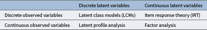

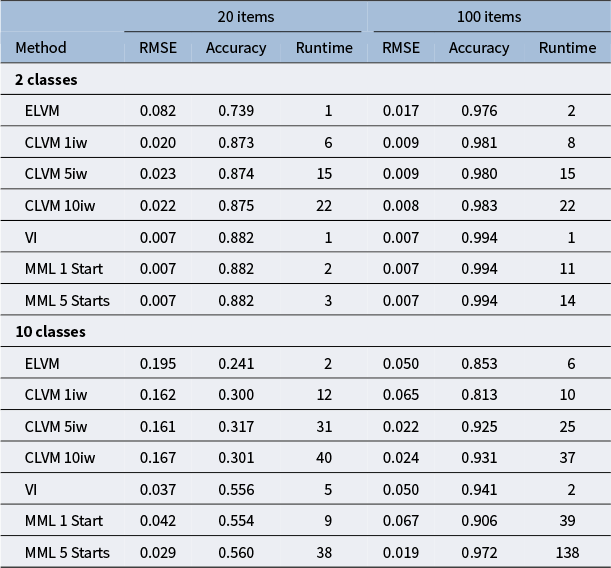
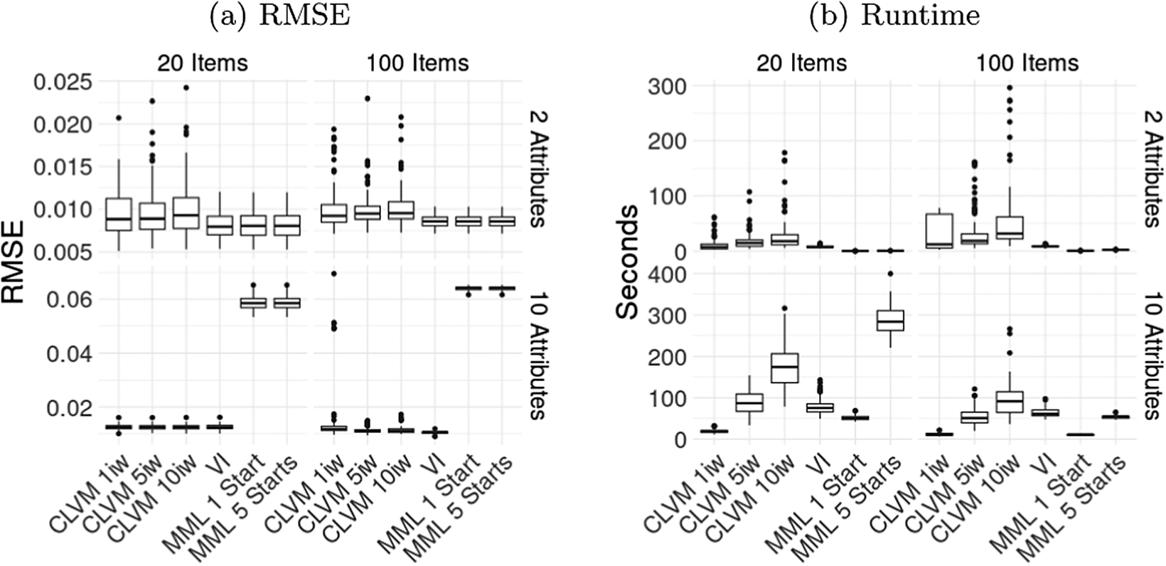

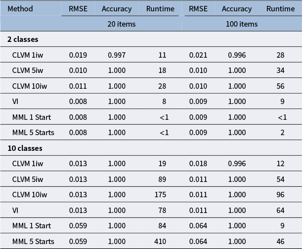
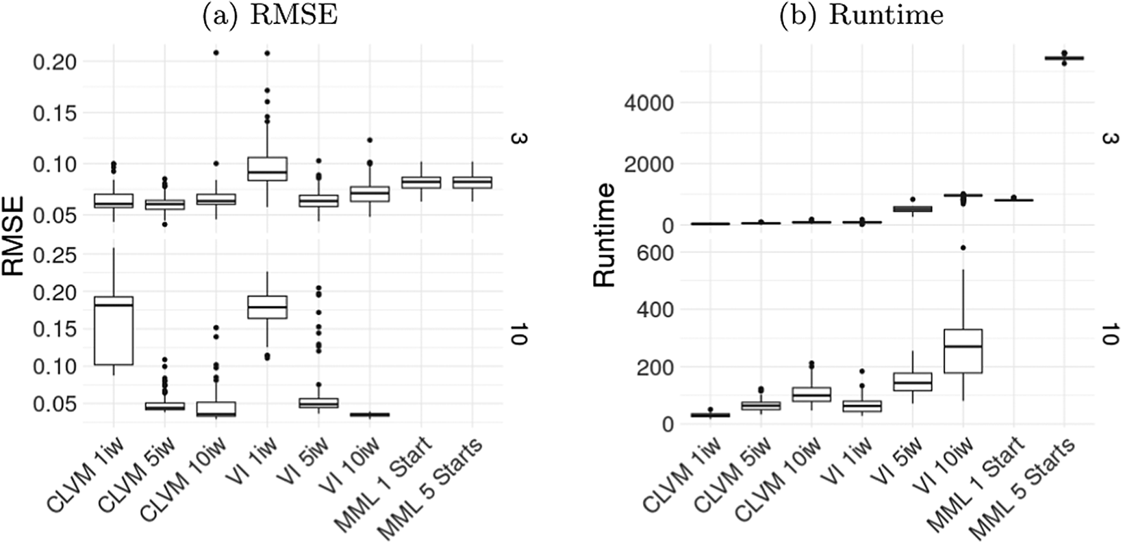
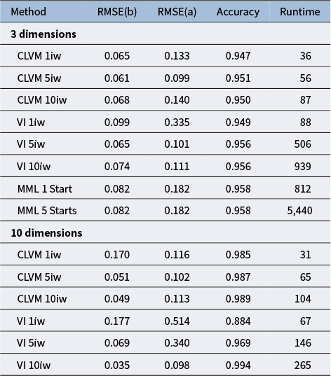


 Open access