


1. Introduction
Source noise (also known as self noise, wave noise, or Hanbury Brown–Twiss noise) arises from the fact that most sources studied in radio astronomy are themselves intrinsically noise-like: that is, stochastic, ergodic, Gaussian random noise (Radhakrishnan Reference Radhakrishnan1999; Thompson, Moran, & Swenson Reference Radhakrishnan2017, 1.2). Since these natural sources are typically very weak relative to other sources of noise (referred to here and elsewhere as ‘system noise’) this contribution can almost always be neglected. However, as telescopes are built with increasing sensitivity, we are more likely to approach or even reach the strong source limit. In this limit (i.e. where the signal strength dominates over other types of noise such that generated in the amplifier) the noise becomes proportional to the signal strength and so the signal-to-noise ratio becomes independent of the sensitivity of the instrument: the only way to increase the signal to noise is to obtain further independent samples by increasing either the bandwidth or observing time. Larger collecting area or more antennas no longer help.
For a single dish, source noise is straightforwardly understood as a contribution to the total noise when the source is in the field of view. For interferometry, the interpretation is a little less straightforward and source noise is better understood as distinct from other noise with distinctive properties. This is because unlike other types of noise, each interferometer element receives the same source noise from an unresolved source (i.e. the source noise is correlated between antennas). It is this correlation which is exploited in an intensity interferometer (Hanbury Brown & Twiss Reference Hanbury Brown and Twiss1954).
This has two important consequences: first, just like the single-dish case, source noise is only seen at the location of the source in either an aperture synthesis image or a phased-array beam. More accurately, in a synthesis image, the noise is distributed with the shape of the instantaneous point spread function (PSF). Second, for an interferometer with a large number of elements, source noise may contribute significantly to the image noise at the location of the source even if it is dwarfed by the system noise of a single interferometer element, since unlike noise which is uncorrelated between elements, the noise cannot be reduced by averaging over baselines.Footnote a
This intermediate regime, where the source is weaker than the noise, but is not weak enough to be negligible, is the subject of this paper. We present a clear detection of source noise (arguably the first in the intermediate regime) in data from the Murchison Widefield Array (MWA; a 128-element low-frequency interferometer; Tingay et al. Reference Melrose2013). We then examine the scenarios in which this may have a negative impact.
The paper is organised as follows: in Section 2, we review the literature on source noise in interferometry and use the formalism obtained to design an experiment to detect source noise with the MWA; in Section 3, we describe the observations and analyse the results; and in Section 4, we discuss the implications of our results.
2. Review of Source Noise
Below, we draw on the literature to describe the properties of source noise. We refer the reader to other articles which discuss the effect of source noise in other specific cases such as pulsar scintillometry (Johnson & Gwinn Reference Johnson and Gwinn2013), spectral line observations (Liszt Reference Liszt2002), pulsar timing (Osłowski et al. Reference Osłowski, van Straten, Hobbs, Bailes and Demorest2011), polarimetry (Deshpande Reference Deshpande1995), or spectropolarimetry (Sault Reference Sault2012). The effect of scattering on source noise is discussed in Codona & Frehlich (Reference Codona and Frehlich1987).
Measurements of the statistics of source noise on very short timescales have also been used to try to detect coherent emission from pulsars (Smits et al. Reference Smits, Stappers, Macquart, Ramachandran and Kuijpers2003, and references therein) In the current work, we focus on the typical synthesis imaging case where a large number of Nyquist samples are averaged in the correlator, and the integration time is far longer than any timescale on which source noise could conceivably be correlated. In this case, the central limit theorem will ensure that source noise is highly Gaussian. We return briefly to this topic in Section 4.3.
Both sources and noise can be described either with a characteristic temperature or as a flux density. We follow Kulkarni (Reference Kulkarni1989) and McCullough (Reference McCullough1993) and use the source flux density S and noise equivalent flux density N throughout. The latter, more commonly known as system equivalent flux density (SEFD), is the flux density of a source that would double the power received by a single element. Thus, at the output of a single element there is the sum of a power proportional to S and power proportional to N, where the constant of proportionality is the product of the collecting area of the antenna, the bandwidth of the receiver, and the antenna gain (and various efficiency parameters). Note that N includes not only receiver noise but also any noise other than S. This is justified below.
Throughout, we assume that all interferometer elements are identical, and that both N and S are stationary, stochastic, and ergodic and so  $2 B \tau$ samples of baseband data are independent. For an unpolarised source, the number of independent samples can be doubled by observing two orthogonal polarisations, so an implicit $n_\mathit{pol}$ can be assumed alongside B and $\tau$ in the equations below. Polarisation of any kind implies correlation of some kind between orthogonal polarisations (Radhakrishnan Reference Radhakrishnan1999) which will complicate the picture. We refer the reader to the references given above for more details on the source noise associated with polarised sources or in polarimetric images.
In the usual case that  $S\ll N$, the RMS noise in a synthesis map is given by
 \begin{equation} \sigma = \frac{N}{\sqrt{2 n_b B \tau}},\end{equation}
where N is the SEFD in jansky,  $n_b$ is the number of baselines given by $n(n-1)/2$ where n is the number of antennas (we assume throughout that all cross-correlations are used), B is the bandwidth in Hz, and $\tau$ is the observing time in seconds.
A similar expression can be derived for  $\sigma$ in the case that one of the antennas is used as a ‘single dish’. In this case, $\sigma$ will be $\sqrt{2}$ higher than for a single-baseline interferometer, since even a single baseline has two antennas and therefore two realisations of noise (see Crane & Napier Reference Crane and Napier1989, Equations (7)–(34)). Equivalently, the noise on a single baseline will be shared randomly between the real and imaginary parts of the visibility, and on average this will reduce the amplitude by $\sqrt{2}$.
In order to understand how the properties of source noise differ from this weak-signal case, it is instructive to examine it in the strong source limit (i.e. where other sources of noise are negligible). Anantharamaiah et al. (Reference Anantharamaiah, Ekers, Radhakrishnan, Cornwell and Goss1989) show that in this case the RMS map noise at the location of the source is simply
 \begin{equation} \sigma = \frac{S}{\sqrt{B \tau}} ,\end{equation}
replicating the single-dish result. This is intuitive since all antennas see the same noise, and so unlike the weak-source case, the noise cannot be reduced by averaging over baselines.
Anantharamaiah et al. (Reference Anantharamaiah, Ekers, Radhakrishnan, Cornwell and Goss1989) derive the properties of source noise in various other regimes to draw a number of important qualitative conclusions.
Firstly, if a strong source is fully resolved on all baselines, then it will be uncorrelated between antennas and so will behave like system noise. This is relevant for low-frequency interferometers such as the MWA where N is actually dominated by Galactic synchrotron emission, which is almost completely resolved on all but the shortest baselines, and totally absent from the longer  $>100\lambda$ baselines typically used for continuum imaging. This provides the justification for lumping sources such as synchrotron radiation from our Galaxy, the cosmic microwave background, and atmospheric noise, etc. in with N, and provides a more precise definition of S as noise which is correlated between antennas.
Secondly, the noise only appears in the image where the source does; therefore, for a point source, the source noise level in the map is shaped like the instantaneous PSF of the array.
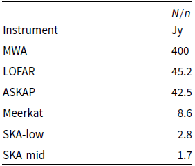
Finally, they note that for an interferometer with n elements, the source noise in the image will be comparable with the system noise when  $N\sim n S$. In Table 1, we list $N/n$ for a number of interferometers to emphasise that this ‘moderately strong source regime’ can easily be reached. $N/n$ for various radio interferometers, built and planned. All come from the SKA baseline designFootnote b Table 1 except the MWA figure which is derived from Tingay et al. (Reference Melrose2013).
Anantharamaiah et al. (Reference Anantharamaiah, Deshpande, Radhakrishnan, Ekers, Cornwell and Goss1991) derive a very simple expression for the noise (system noise and self noise) at any location in the map for a total power image. We modify this slightly so that it simplifies to Equations (1) and (2) in the appropriate limits:
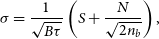 \begin{equation} \sigma = \frac{1}{\sqrt{B\tau}}\left(S + \frac{N}{\sqrt{2 n_b}}\right),\end{equation}
where S is the apparent source brightness (source brightness distribution convolved with the PSF) at any point in the image.
This expression is only approximate for an interferometry image because it does not account precisely for how the noise on different baselines is correlated in this 'moderately strong source' regime. A more complete treatment was given by Kulkarni (Reference Kulkarni1989), who considered the correlation between each pair of baselines. Three classes of baseline pairs were identified: the autocorrelations of each baseline, those where the pair of baselines have an element in common, and those where the pair of baselines is composed of four different antennas. Source noise correlates between the baselines differently in each case. For a point source at the phase centre, the visibility on each baseline is identical, and the on-source noise is
 \begin{equation} \sigma = \frac{S+N}{\sqrt{2 n_b B \tau}}\sqrt{1 + 2\left(n\!-\!2\right)S' + \left[1 + \left(n\!-\!1\right)\left(n\!-\!2\right)\right]S'^2},\end{equation}
where
 \begin{equation} S' = \frac{S}{S+N} .\end{equation}
Here we use the form of the equation given by McCullough (Reference McCullough1993) who corrected a minor error in Kulkarni (Reference Kulkarni1989). The three terms reflect the three classes of baseline pair: the autocorrelations will correlate perfectly regardless of whether S or N dominates and the other two classes scale with S’ and  $S'^2$, respectively.
Equation (4) reduces to Equation (1) or (2) in the appropriate limits. It is also well-approximated by Equation (3) for large n as predicted by Anantharamaiah et al. (Reference Anantharamaiah, Deshpande, Radhakrishnan, Ekers, Cornwell and Goss1991) (the fractional error is  $<1\%$ for $n>12$).
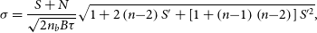
Figure 1 shows the achievable dynamic range (signal-to-noise) off- and on-source (i.e. calculated using Equations (1) and (4), respectively). The source brightness is given in units of  $N/n$ (see Table 1). On- and off-source noise starts to diverge at $\sim N/10n$—just a few hundred mJy for the SKA, and the on-source dynamic range has almost reached its maximum value by $\sim 10N/n$.
Following Kulkarni (Reference Kulkarni1989) Figure 2, maximum achievable dynamic range achievable off-source (dashed line; Equation (1)) and on-source (solid line; Equation (3)) for as a function of source strength for a large-n interferometer. This is generalised by measuring source flux density in units of  $N/n$ and dynamic range as a fraction of its maximum ( $\sqrt{B\tau}$).
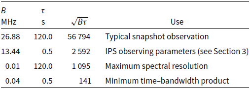
Table 2 shows the maximum dynamic range obtainable for various common MWA observing parameters. For a typical snapshot, the dynamic range will be  $> 10^4$ before source noise effects become noticeable. This level of source noise is not easily measured since noise due to confusion noise or calibration errors are likely to limit the dynamic range far more.
In contrast, if an image is made with the smallest possible bandwidth and observing time with the current MWA correlator, the maximum achievable dynamic range is  $\sim$100. Solar images are regularly made in this way with the MWA, and the quiet Sun flux density at 150 MHz is sufficiently far into the strong source regime that even if this flux density is spread over many pixels the brightness of each resolution unit to be close to the strong source regime. This means that every resolution unit of the Sun will fluctuate by $\sim$1% across timesteps, spectral channels, and polarisations regardless of any intrinsic change in brightness. However, rapid intrinsic changes in solar emission (which may be polarised) in both time and frequency would complicate measurements of source noise in observations of the Sun.
Both spectral line and 0.5 s snapshot imaging will start to show the effects of source noise at dynamic ranges  $\sim$1 000. Thus, if images could be made for each of a large number of spectral channels or timesteps, the RMS of pixels on- and off -source would be expected to show a measurable difference. The former is the approach taken by McCullough (Reference McCullough1993) in measuring source noise in the strong regime. We take the latter approach which has much in common with the procedure used for making interplanetary scintillation (IPS) observations with the MWA (Morgan et al. Reference Morgan2018). $\sqrt{B\tau}$ for various MWA observing modes. All bandwidths take into account discarded band edges where appropriate. Maximum resolutions in time and frequency refer to the original online MWA correlator (still standard at the time of writing).
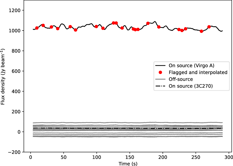
Timeseries (lightcurve) showing brightness of various pixels in the image as a function of time. Black line shows the on-source lightcurve; dot-dashed black line shows a much weaker source: the (Western lobe of) 3C270; grey lines show a selection of off-source pixels. Twenty-one points in the lightcurve had to be flagged due to clearly discrepant points, and these have been linearly interpolated over in all lightcurves; red circles denote these flagged points for the on-source pixel.
3. Observations
As part of our IPS observing campaign (Morgan et al. Reference Morgan, Macquart, Chhetri, Ekers, Tingay and Sadler2019) we observed a series of calibrators in high time resolution mode with 5-min observing time. These observations pre-date the upgrade of the MWA to Phase II (Wayth et al.Reference Wayth2018). Virgo A (M87), at our observing frequency of 162 MHz, was observed at 2016-01-16T21:04:55 UTC when it was 53 degrees above the horizon and 112 degrees from the Sun. The solar elongation is relevant since Virgo A has a compact core and jet several janskys in brightness at GHz frequencies (e.g. Reid et al. Reference Reid, Schmitt, Owen, Booth, Wilkinson, Shaffer, Johnston and Hardee1982) which would be compact on IPS scales. This means that Virgo A will also show IPS. However, this variability should be fully resolved with 2 Hz sampling. Throughout, we assume a flux density of 1032 Jy for Virgo A (based on values gleaned from the literature by Hurley-Walker et al. Reference Hurley-Walker2017). We do not include any uncertainty on the flux density of Virgo A in our errors below (such an error would cause an equal scaling error in all of our measured and derived quantities). Note that no direction-dependent flux scaling was carried out.
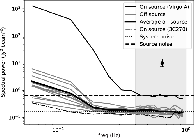
Power spectrum for each of the lightcurves described in Figure 2. The thin black line shows on-source power spectrum; the dot-dashed line shows a much weaker source (3C270); the grey lines show off-source power spectra, with the thick black line showing the average of the grey lines. Power spectrum parameters are described in the text. The single error bar shows the 95% confidence interval for a single point with these parameters. The dotted line is the mean of all off-source power spectrum points above 0.4 Hz. The dashed line is the estimate of the on-source power based on the on-source brightness and off-source noise.
Each individual 0.5 s integration of the full observation was imaged separately for each instrumental polarisation (XX and YY) using normal weighting and excluding baselines shorter than 24- $\lambda$ (a negligible fraction of the total number of baselines). Throughout this paper, we only refer to results derived from the XX images; however, using the YY images produces qualitatively identical results. Figure 2 shows the lightcurves for selected pixels in the image: the pixel corresponding to the brightest point in Virgo A and several pixels distributed through the image a few resolution units from Virgo A. Additionally, we show a pixel corresponding to the brightest point in 3C270, a resolved double with a peak apparent brightness approximately 3% of that of Virgo A. After standard flagging of the start and end of the observation, 573 timesteps remained. A number of clearly discrepant points were easily discernible in all lightcurves (the same in each) and these have been interpolated over for all lightcurves. The on-source lightcurve shows clear variability on a timescale consistent with ionospheric scintillation.
Figure 3 shows power spectra for each of the lightcurves shown in Figure 1. These were generated using Welch’s method (Welch Reference Welch1967) with 17 overlapping FFTs of 32 samples with a Hanning window function. The strong signal that dominates at low frequencies is consistent with ionospheric scintillation and shows the characteristic Fresnel ‘Knee’ at about 0.1 Hz. Above this frequency the power drops steeply. The same ionospheric scintillation can be seen for all off-source lightcurves due to the sidelobes of Virgo A; however, the sidelobes level is low enough that the variance is suppressed by at least three orders of magnitude. 3C270 scintillates independently of Virgo A and also has a slightly lower noise level.Footnote c
Above 0.4 Hz the variance from ionospheric scintillation is negligible, and the power spectrum consists only of white noise. We conclude that all variability due to calibration errors such as those introduced by the ionosphere is restricted to lower frequencies as we would expect. This white noise is clearly at very different levels on-source and off-source. We can use the average of all points above 0.4 Hz to measure the off-source noise to be 0.410 $\pm$0.005 Jy and the on-source noise to be 0.75 $\pm$0.03 Jy. The former implies that the SEFD (N) is 125 000 $\pm$1 500 Jy ( $B=13.44$ MHz, $\tau=0.5$ s, $n=118$, i.e. 10 antennas flagged). This is about a factor of 2.4 higher than that given in Table 1, which is not surprising given the off-zenith pointing and the fact that Tingay et al. (Reference Melrose2013) assume a nominal sky temperature and field of view.
Using the source brightness and off-source noise, we can calculate what the on-source noise should be using Equation (4). This prediction (0.807 $\pm$0.005 Jy) is shown as the dashed line in Figure 3 and it agrees extremely well with the measured on-source noise. There is a small discrepancy, which is within 2- $\sigma$; however, even this small excess can be explained as a small leakage of source noise into the off-source pixels due to the sidelobes of Virgo A. Alternatively, this may be due to Virgo A being slightly resolved on some MWA baselines.
This does not leave any variance due to IPS. IPS is extremely variable on the night-side, and the scintillation index would only be a few percent. Furthermore, most of the variability is on timescales longer than 0.4 Hz. IPS may be responsible for the slight increase in power around 0.3 Hz.
3C270 does not exhibit measurable source noise. This is expected since, like the sidelobes of Virgo A, its brightness puts it well within the weak regime.
4. Discussion
We have detected source noise at a level which is firmly in line with the predictions of Equation (3) (no empirical test for the existence of the subtle effects that differentiate Equations (3) and (4) is possible with our data since the two are practically identical for  $n>100$). We now consider the effect that this would have off-source in synthesis images.
4.1. The leakage of source noise off -source
Figure 4 plots the ratio of on-source noise to system noise where these are calculated using Equations (3) and (1), respectively. To understand the effect this has off-source, consider a narrowband snapshot image. In this case, the source noise will have the shape of the snapshot, monochromatic PSF. The sidelobes of this PSF can be characterised by their RMS relative to the central peak; for example, the proposed SKA-low configurationFootnote d has a sidelobe level of 1% in the instantaneous monochromatic case. Therefore for  $S=N/n=2.7$ Jy, the source noise level on-source will be $\sim2\times$ the weak-noise level, and off-source this 100% increase in noise will become just 1%.

As the bandwidth and integration time are increased, both the system noise and the source noise will reduce with  $\sqrt{B\tau}$ the ratio between the two will remain constant, and the excess noise due to the source noise will remain at $1\%$. With appreciable fractional bandwidth and/or Earth rotation synthesis, this source noise will be spread smoothly over the image.
For the example given, the effects of source noise off-source are extremely low; however, there will be 5 $\times$ 2.7 Jy sources per FoV with the SKA-low (Franzen et al. Reference Franzen2016). For a 14 Jy source ( $\sim$1 per FoV), there would be an excess of 5%. Only for a 270 Jy source will the noise be doubled and such sources are relatively rare for extragalactic fields assuming arcminute or better resolution.
Two effects will reduce the impact of source noise even further. First, the 1% level given for the SKA-low case is for the 100 resolution units closest to the source. The sidelobe level will drop even lower with increasing distance from the bright source. Second, this level of source noise assumes natural weighting of baselines. More uniform weighting will increase the weighting of certain baselines (the longer ones) by a large amount compared to the shorter spacings, particularly for instruments like the SKA-low with very high concentrations of collecting area at the centre. This will reduce the effective number of antennas and therefore the source noise relative to the system noise.
4.2. Subtracting source noise
Anantharamaiah et al. (Reference Anantharamaiah, Ekers, Radhakrishnan, Cornwell and Goss1989) note that source noise can be subtracted perfectly from a snapshot by deconvolution, while noting the computational effort required to do so. Here we explore the limitations on how cleanly this can be done.
Subtracting source noise requires that the field be imaged with sufficient time and frequency resolution for changes in the PSF to be insignificant from one image to the next. The required resolution will depend on the array and imaging parameters; however, the requirements are similar to those required to minimise time-average and bandwidth smearing (e.g. Thompson et al. 2017, 6.3–6.4) and are likely to be demanding. Here we concentrate on a more fundamental issue that such a subtraction poses: namely that if the source noise is to be perfectly subtracted, the source brightness must be allowed to vary as a function of time and frequency and no spectral smoothness can be assumed. Conversely, if spectral smoothness is strictly imposed, as is normally the case when subtracting continuum from spectral line cubes, no source noise will be subtracted. Clearly, any number of compromised schemes between these two extremes could be devised; however, the principle remains that source noise can only be subtracted to the extent that it can be separated from any spectral or temporal signal that needs to be preserved.
4.3. Conclusion
The properties of source noise lead us to the striking conclusions that the SKA will not more accurately characterise a 1 000 Jy source than a 10 Jy source, and that the standard equations underestimate the noise on the measurement of a 2 Jy source by a factor of two. We have demonstrated that even the MWA—which is orders of magnitude less sensitive than the SKA—can measure these effects at the 12- $\sigma$ level (albeit it in an observation of a 1 000 Jy source contrived for the purpose).
Our observations show that the magnitude of the effect is precisely in line with predictions, and so source noise can be predicted very precisely from easily measurable parameters (the ratio of source brightness to system noise). This is in contrast to other sources of variability such as the ionosphere. Source noise is also expected to have stochastic behaviour as a function of frequency and time, and we exploit this to separate source noise from much stronger ionospheric effects.
Although the effects on standard continuum imaging appear to be benign in all but the most extreme cases, source noise could become problematic wherever weak signals (including polarised signals, see Sault Reference Sault2012) need to be measured in the presence of strong emission, especially where the signals involved have fine frequency structure or vary on short timescales. This situation will occur for any spectral line observations where the continuum has to be subtracted to see the much weaker line emission. In this situation, the noise will be higher and not uniform across the image. Noise estimates made from regions of the image with no continuum will underestimate the noise.
Fast transients such as fast radio bursts (FRBs) and pulsars will also reach the strong source limit, especially since their signals occupy only a narrow sloping band in a dynamic spectrum. For ASKAP, a few of the detected FRBs (Shannon et al. 2018) already have peak flux density in the strong source limit and for SKA sensitivity many will be in this regime. Thus, measurements of source noise of FRBs should be possible, and such measurements may be valuable, since they probe the extent to which the emission is coherent (Melrose 2009).
Acknowledgements
We would like to thank J-P Macquart, Adrian Sutinjo, and Wasim Raja for useful discussions. This scientific work makes use of the Murchison Radio-astronomy Observatory, operated by CSIRO. We acknowledge the Wajarri Yamatji people as the traditional owners of the Observatory site. Support for the operation of the MWA is provided by the Australian Government (NCRIS), under a contract to Curtin University administered by Astronomy Australia Limited. We acknowledge the Pawsey Supercomputing Centre which is supported by the Western Australian and Australian Governments.


