

1. Introduction
The movement of alpine glaciers results from a number of complex, coupled mechanisms involving hydrology, mechanics and thermodynamics on microscopic to kilometre-sized scales. This movement is strongly controlled by the friction at the base of the glacier, and is therefore difficult to observe directly. Many authors have made use of boreholes to study basal processes. Borehole instrumentation allows for monitoring changes in water pressure, sliding rate and bed strength variations at the base of glaciers (see Reference ClarkeClarke, 2005, for a review of studies using boreholes instrumentation). However, studies employing these methods are of low resolution since only a few localized spots are sampled. Some rare examples of subglacial laboratories in France (Reference VivianVivian, 1971) and in Norway (e.g. Reference Jansson, Kohler and PohjolaJansson and others, 1996) allow access to the base of the glacier and hence direct observation of subglacial processes. Reference Kamb and LaChapelleKamb and LaChapelle (1964) dug a tunnel in the ice to the bedrock especially for this purpose. Such sites or experiments only probe the glacier base at certain localized spots, however, which may be neither typical nor the most interesting or important ones.
Apart from these exceptions, there is no way to directly measure basal processes. Consequently, different geophysical remote-sensing methods have been applied to glaciers. Ground-penetrating radar (Reference Plewes and HubbardPlewes and Hubbard, 2001) and active seismic methods (Reference CraryCrary, 1963) are the most commonly used to investigate ice thickness and the internal structure of the glacier. However, these methods provide little information about basal sliding processes. Passive seismic methods have proved useful in the study of basal processes, especially as they can remotely probe the in situ mechanical properties of the glacier and its base over larger length scales than tunnels or boreholes.
In their early works, Reference Neave and SavageNeave and Savage (1970) reported that the opening of crevasses was the only source for the seismic activity they recorded. However, Reference Weaver and MaloneWeaver and Malone (1979) found low-frequency events that, as they suggested, could be related to basal processes such as stick–slip sliding. Other studies confirmed these results despite a low accuracy in event location (Reference Deichmann, Ansorge and RöthlisbergerDeichmann and others, 1979).
More recently, Reference Blankenship, Anandakrishnan, Kempf and BentleyBlankenship and others (1987) and Reference Anandakrishnan and BentleyAnandakrishnan and Bentley (1993) revealed the existence of seismic events associated with stick–slip at the base of Ice Streams B and C, West Antarctica, both being soft-bedded glaciers. Reference Ekström, Nettles and AbersEkström and others (2003) mentioned glacial earthquakes associated with large stick–slip processes that may occur at the base of the Greenland and Alaska glaciers, and Reference Deichmann, Ansorge, Scherbaum, Aschwanden, Bernardi and GudmundssonDeichmann and others (2000) also identified evidence for deep icequake occurrences in Unteraargletscher, Bernese Alps, Switzerland.
Theoretical studies on basal processes (Reference WeertmanWeertman, 1957, Reference Weertman1964; Reference LliboutryLliboutry, 1968) postulate that regelation and plastic flow are the two main processes governing basal sliding. Regelation theory states that on the upstream side of an obstacle in the glacier bed there is an excess of pressure that lowers the pressure-melting point and apparently cools the ice (assumed to be at the pressure-melting point and to be separated from the bedrock by a thin water film). Heat therefore flows from the downstream to the upstream side either through the rock or the surrounding ice, melting ice on the upstream face. The meltwater flows around the obstacle and refreezes on the downstream side. However, this theory relies on four basic assumptions that are not consistent with reality (Reference WeertmanWeertman, 1957). More realistic models have been developed since then (Reference WeertmanWeertman, 1964; Reference KambKamb, 1970; Reference NyeNye, 1970; Reference LliboutryLliboutry, 1987), but they are still inconsistent with measured ice velocities (e.g. Reference IkenIken, 1997).
None of these theories predict unsteady sliding such as stick–slip motion, since they assume zero friction at the ice– bed interface. Reference RobinRobin (1976) suggested that the meltwater could be squeezed out of the upstream ice and could therefore produce patches of cold ice freezing to the bedrock. These cold patches could contribute to basal friction (as could rocks in the basal ice), leading to the jerky motion mentioned by some authors (Reference Vivian and BocquetVivian and Bocquet, 1973; Reference HubbardHubbard, 2002).
The microseismic activity of an alpine glacier should reveal highly stressed zones that can be linked with basal friction. It is, however, necessary to separate surface activity (opening and widening of crevasses) from deeper seismic activity. In this paper, we address the problem of source location of icequakes by using an array technique (for a review of classical array techniques, see Reference Rost and ThomasRost and Thomas, 2002). We propose a method of source location and characterization using a grid search approach. We took advantage of the galleries under the base of Glacier d’Argentière, Mont Blanc, France, to set up a network of seismometers deployed as antennas in order to measure the seismic activity from the base. We therefore have the opportunity to measure the deeply sourced signals that can be masked from surface measurements by emissive crevasse processes. For each pair of seismometers of a given antenna, the time delays are measured and then compared to the theoretical delays calculated by tracing rays between each point of the data elevation model and the sensors of our network. A description of the different steps of the procedure is presented and the method is applied to our dataset. Icequake magnitudes are also computed. We find evidence for patches of high seismic activity which suggests that basal friction produces heterogeneous stress zones (at least in this part of the glacier). A link is made between these results and previous theoretical and practical studies of basal processes.
2. Measuring Microseismic Activity at Glacier D’Argentière
Glacier d’Argentière is a 10 km long temperate glacier located in the Mont Blanc Massif in Haute Savoie, France. Its surface area is 19 km2 and its maximum and minimum altitudes are 3400 and 1700 m a.s.l. respectively. A large change in the slope of the bedrock has created a serac fall 2 km up-glacier from the snout. Because of the overall shrinking of the glacier, the bedrock can be seen in the middle of the serac fall (Fig. 1). Behind the serac fall, a network of industrial cavities or galleries has been dug into the bedrock about 5 m under the glacier bed by Emosson S.A. (hydroelectric power company) at 2170 m a.s.l. The mean thickness of ice above the galleries is around 100 m (Reference Reynaud, Donnou, Perrin, Rado, Ribola and VincentReynaud and others, 1988). A detailed section of the serac fall and more details of the galleries are given by Reference VivianVivian (1971) and by Reference Vivian and BocquetVivian and Bocquet (1973).

Fig. 1. The glacier flows approximately south to north. The white triangles represent the seismometers used in this study, numbered 1–9 (from right to left). The black triangles show the six seismometers that are not used in this study.
Two seismic experiments were carried out at Glacier d’Argentière during April 2002 and between 10 December 2003 and 21 January 2004. We report data measured during the 2003/04 winter campaign, during which a network of seismic arrays was set up in one of the galleries (shown as thick line crossing the glacier in Fig. 1). It comprised fifteen 1 Hz Mark Products L4-C seismometers operated on three-channel seismic recorders. Sensors were spaced ∼50 m apart (Fig. 1).
In this paper, we report results using only nine out of fifteen seismometers, as two recorders did not work properly. Also, the three recorders considered did not have the same time base. This led us to process each of the three remaining stations as separate antennas, made of three seismometers each. We thus have at our disposal nine pairs of sensors (three pairs per recorder). Furthermore, all sensors lie at the same altitude, yielding a poor resolution in depth.
Simultaneous and continuous recordings with sampling frequency 250 Hz were obtained at the three recorders from 11 December 2003 to 9 January 2004.
3. Signal Characteristics
The data show a very high seismic emissivity from the glacier. At least two main types of events can be observed, referred to as type I and II. Most type I events are due to small cracks and show a short, impulsive signal (type I event, Fig. 2). Type I ice-quakes lie within the 10–40 Hz band and therefore represent relatively high-frequency events. Since the seismometers are close to the sources, attenuation is low even at these frequencies. Type II observations are composed of long, complex signals with high amplitude that are likely to be associated with serac falls. The frequency content of this type of icequake is more complex than that of type I events and varies with time (Fig. 3b,d,f and h). Unfortunately, visual observation is the only way to prove such events are serac falls. However, we are able to localize them and thus show that they happen where we expect them to (see Fig. 9, shown later).

Fig. 2. (a) Unfiltered velocity seismogram of a type I icequake recorded at channel 1 (maximum amplitude 0.84 μm s−1), and (b) corresponding smoothed normalized power spectrum density.

Fig. 3. Velocity seismograms of a type II event recorded at channel 1, and the corresponding power density spectra. The top window (a) shows the entire serac fall signal, lasting for more than 15 s. Boxes marked (b), (d), (f) and (h) are sub-events, shown in more detail in respective windows with corresponding spectra (c, e, g, i) on their right.
Grouping seismic events into two main types is approximate, as it is possible to find events of an intermediate type. In all cases, it is impossible to distinguish primary (P) from secondary (S) wave arrivals. We found some rare examples of events showing a possible P wave, therefore confirming the hypothesis that the measured wave train is the S wave. Another possibility would be surface waves, propagating along the ice–rock interface; we have no way to confirm this, however. As a consequence, we suppose S wave energy is dominant in the recorded signals.
We can also find a few low-frequency events which are regional tectonic earthquakes. Some of these were also recorded by SISMALP (French Alps Seismic Network) (Reference Thouvenot, Fréchet, Guyoton, Guiguet and JenattonThouvenot and others, 1990; Reference Thouvenot, Fréchet, Pinter, Gyula, Weber, Stein and MedakThouvenot and Fréchet, 2006), while others were only recorded on the Argentière array as their amplitude was too small to trigger SISMALP. Many icequakes (whatever their type) show quasi-harmonic codas peaked at around 21 Hz (Fig. 3h and i). The value of this peak frequency is dependent on the sensor. Table 1 lists these different values for the nine seismometers. Note that these resonances are not necessarily recorded on all nine seismometers. It appears that the L4-C seismometers can generate such a resonance in specific conditions (e.g. when being excited by nearby sources). We therefore attribute this resonance to an instrumental response rather than a physical feature of the glacier.
Table 1. List of frequency peak values measured at each station of our network (the stations are ordered geographically according to Figure 1). Although these values are different for all nine seismometers, they remain constant in the time interval considered in our study (approximately 1 month)

4. Detection Event Statistics
Using a short-term average over long-term average (STA/LTA) method (Reference AllenAllen, 1978) with parameters STA window length = 0.7 s, LTA window length = 7 s and threshold = 1.5, we quantified the high emissivity from the glacier. We systematically added a 1 s pre-event window to avoid missing first arrivals on certain channels, and a 3 s post-event window to ensure the full waveform is taken into account. Furthermore, we only analyzed events that were simultaneously recorded on the nine seismometers.
A total of 13 390 icequakes of all types were detected via this method. From these, it is possible to separate the serac falls (type II events) by applying duration and amplitude criteria. To do so, we merged overlapping events in order to compute a duration. The events with a duration of longer than 10 s (taking into account the pre- and post-event time lags introduced at the detection step), and with a maximum peak-to-peak amplitude greater than 2.42 μm s−1 on two sensors simultaneously, were considered to be serac falls. The two sensors were chosen in order to ensure both a good signal-to-noise ratio and proximity to the Rognon where the serac falls were expected to be located. These duration and amplitude thresholds were chosen empirically. With these criteria, 32 major serac falls were detected.
Figure 4 shows the number of detected events per hour and the cumulative number of icequakes over the 30 day period. The seismic rate is relatively constant from 11 to 29 December 2003 and then decreases. There are small variations, with a major peak at 22–23 December (Fig. 4). This event corresponds to two events (at around 1600 and 1900 h) on 22 December when a strong increase in the number of high-amplitude icequakes (both type I and type II events) is observed over about 20 min. One of these two swarms is shown in Figure 5. The increase of high-amplitude icequakes is clearly seen. These swarms are not due to human activity since they are recorded on the nine seismometers of the network and occur out of working hours in the galleries.

Fig. 4. (a) Number of detected events per hour over the 30 days, and (b) cumulative number of events. An episode of anomalously high seismic activity occurred on 22 December, shown by the vertical lines.

Fig. 5. (a) Cumulative number of detected events from 1600 to 1700 h on 22 December. (b) One hour of signal on channel 1; the peak velocity is indicated in the lower lefthand corner. This swarm seems to lead to a major event of high amplitude, followed by a few smaller events.
The mean number of events per hour was 19.34 over the 30 day period. In order to take into account the change in the seismicity rate occurring by the end of December, we computed the mean number of events per hour for two separate periods (Fig. 6). The null hypothesis of a stationary Poisson law requires that the number of events N occurring during 1 hour follows a Poisson distribution with a mean λ. Averaging over n days, the sample mean number (N
1 + N
2 + … + Nn)/n must then have a mean λ and a standard deviation ![]() . The Poisson mean is calculated using the number of events per hour for the two separate time periods (21 days and 7 days for the December and January period, respectively). A mean number of events of 23.5 h−
1 with a standard deviation of
. The Poisson mean is calculated using the number of events per hour for the two separate time periods (21 days and 7 days for the December and January period, respectively). A mean number of events of 23.5 h−
1 with a standard deviation of ![]() is obtained for the first period, while for the second period the mean number of events is 8.33 h−
1 with a standard deviation of
is obtained for the first period, while for the second period the mean number of events is 8.33 h−
1 with a standard deviation of ![]() . In both cases we see that the mean number of events per hour is close to a Poisson law, with only one remarkable departure in January (between 0100 and 0200 h). We cannot find any clear day/night cycle in the temporal variation of the seismic activity. It should be noted that the galleries are visited by workers on a daily basis, and so some events are due to this human activity. Nevertheless, since we imposed the criterion that an event must trigger all seismometers simultaneously, these human-related events can be neglected in our analysis. Furthermore, this human activity is relatively low during the winter period.
. In both cases we see that the mean number of events per hour is close to a Poisson law, with only one remarkable departure in January (between 0100 and 0200 h). We cannot find any clear day/night cycle in the temporal variation of the seismic activity. It should be noted that the galleries are visited by workers on a daily basis, and so some events are due to this human activity. Nevertheless, since we imposed the criterion that an event must trigger all seismometers simultaneously, these human-related events can be neglected in our analysis. Furthermore, this human activity is relatively low during the winter period.

Fig. 6. Comparison of the mean number of events per hour computed over (a) December and (b) January (circles). The mean (solid line) plus or minus standard deviation (dashed line) is shown in both cases. There is no clear day/night cycle, nor any link with human activity in the galleries.
5. Computation of Time Delays
An array is a network of sensors close to each other in order to record a delayed but coherent signal on each. Arrays were originally used to detect and identify nuclear explosions (Reference Mykkeltveit, Ringdal, Kværna and AlewineMykkeltveit and others, 1990), but quickly expanded to other applications in seismology (for a review of array techniques and their possible applications see Reference Rost and ThomasRost and Thomas, 2002). These methods have been used in volcano seismology (Reference Chouet, Scarpa and TillingChouet, 1996; Reference Almendros, Ibáñez, Alguacil and Del PezzoAlmendros and others, 1999) and allow the computation of the precise time delay between pairs of seismometers of a given recorder. The geometry of an array is usually determined according to the particular application. However, in our case, the geometry of the array is imposed by the geometry of the galleries.
Time delay computation is more precise than phase picking, especially as it is impossible in this case to distinguish between P- and S-wave arrivals (see section 3). There are different methods of computing the time shift between two coherent waves. They usually rely on the coherency function in the frequency domain (Reference Jenkins and WattsJenkins and Watts, 1968) or cross-correlation function in the time domain (e.g. Reference Frankel, Hough, Friberg and BusbyFrankel and others, 1991). Here, we used a simple method of delay computation in the time domain that is independent of spectral analysis parameters (analysis-window sizes) but which still yields a precision in time delay measurement that is below the sampling rate.
We compute the time delay by minimizing the normalized root mean square (rms) of the difference of two shifted signals arriving at two sensors of a given antenna. Let si and sj be the centred signals recorded on seismometers i and j and let Rij be the rms function defined as
where ![]() and
and ![]() are the variances of signals i and j respectively, τ is the time lag, N is the number of samples in the considered signal and tk
is the kth sample. Hence, when the time shift corresponds to the physical delay, the rms tends to zero, assuming that the signals are coherent enough. For uncorrelated signals, Rij
tends to 1 in the limit of infinite samples (N → ∞).
are the variances of signals i and j respectively, τ is the time lag, N is the number of samples in the considered signal and tk
is the kth sample. Hence, when the time shift corresponds to the physical delay, the rms tends to zero, assuming that the signals are coherent enough. For uncorrelated signals, Rij
tends to 1 in the limit of infinite samples (N → ∞).
Initially, the tested time shifts τ are multiples of the sampling period. A quadratic interpolation is performed on this discrete rms function in order to determine the position of the minimum, hence yielding the final value of the time lag with precision below the sampling rate of 4 ms (Fig. 7). The difference between the minima of the interpolated and the discrete rms function (Fig. 7) is due to the number of points used in the interpolation. The resolution of the interpolation decreases if fewer points are used; we used 10 points centred around the initial minimum. The minimum value of the rms function indicates if the two signals are coherent, and therefore if the value of delay is of good quality. Typical values for this minimum range from 0.4 to 0.7, preventing us from forming a reliable criterion.

Fig. 7. (a) Signal of a type I event recorded on seismometers 1 (solid line) and 2 (dashed line) separated by ∼40 m. (b) Normalized discrete rms function (dotted line) and interpolated rms function (solid line) vs time lag. The former yields a precision below the sampling period of 4 ms.
We applied this technique to the 13 930 detected events. They were bandpass-filtered by multiplying their Fourier transform by a Gaussian with mean 20 Hz and standard deviation 20 Hz in order to attenuate high-frequency noise. The delays of 13 716 events were calculated. Given the geometry and the number of recorders and sensors available, we compute nine values of delays for each event (i.e. three pairs of seismometers on three different recorders).
6. Locating the Sources
The time delay between seismometers i and j can be expressed by the difference between the travel times:
where τij is the time delay between sensors i and j, Ti and Tj are the travel times from source to sensors i and j, respectively, P i and P j are paths between the source and sensors i and j respectively, v is the velocity and s is the coordinate along the ray. The time delay thus depends on the source and receiver positions and on the velocity model in which the wavefield propagates. However, since the sensors are close to each other, the time lag is mostly due to the difference of wave path in the medium close to them.
The influencing velocity parameters are therefore: (1) the contrast between ice and rock wave velocities that will determine the transmission angle at the interface, and (2) the wave velocity close to each seismometer. Since we do not have much information on heterogeneities of either propagation medium, and in order to simplify the problem and to decrease the number of unknowns, we approximate the velocity model by supposing the ice and the rock are both homogeneous. The ice mass at a serac zone is, however, a highly fractured medium. Yet this hypothesis is valid as long as the wavelength of the considered waves is much greater than the size of the fractures. A simple order-of-magnitude calculation yields a wavelength ranging from 50 to 130 m using a wave velocity of 2000 m s−1. These values are higher than classical values for ice fracturing that can be found in temperate glaciers; the largest crevasse that can be found at Glacier d’Argentière is around 20 m wide.
The sources are localized by performing a two-step grid search. A digital elevation model (DEM) was constructed based on measurements collected by the Emosson company for the topography of the bedrock and the spatial changes in ice thickness, and by the Institut Géographique National, France, for the glacier surface topography. Since these topographical data pre-date our experiment, we apply a homogeneous decrease of 10 m to the ice thickness over the whole glacial surface. This value is constrained to be consistent with the observed size of the bare rock patch (the Rognon) that is apparent in the middle of the serac zone. The spacing of the DEM is 30 m. Seismic wave velocity in ice has already been measured for temperate glaciers (Reference Weaver and MaloneWeaver and Malone, 1979; Reference Deichmann, Ansorge, Scherbaum, Aschwanden, Bernardi and GudmundssonDeichmann and others, 2000), but these measurements were made from the surface on homogeneous parts of the glaciers. In our case, however, we can suppose that the effective seismic wave velocity at the serac fall might be lower than the value measured in the former studies since it is a highly fractured medium occasionally filled with water or air. Similarly, the seismic wave velocity close to the array is unknown, as the rock was decompressed by the excavation of the galleries. Since no precise measurement of wave velocities has been carried out at Glacier d’Argentière, we consider these velocities in both ice and rock as unknowns.
Each point in the ice (and a few points belonging to Rognon) of this DEM is considered as a possible location for a given icequake. We trace the ray between this point and each of the nine seismometers for different velocity models. Ice velocities are constrained to range from 1000 to 2500 m s−1 and rock velocities from 1800 to 2800 m s− 1, both with a step of 50 m s− 1. We also impose a lower seismic wave velocity in ice than in rock. This ray-tracing task is performed using an enhanced Podvin–Lecomte algorithm (Reference Podvin and LecomtePodvin and Lecomte, 1991; Reference Monteiller, Got, Virieux and OkuboMonteiller and others, 2005). We then calculate theoretical time delays for each of the velocity models considered. This theoretical value is to be compared to the measured value by minimizing the error function:
where ![]() and
and ![]() are the calculated and the observed time delay for sensors i and j, respectively, and σij
is the standard deviation of delay measurements for sensors i and j. This standard deviation must take into account both the precision of time delay measurements (half of the sampling rate set at 4 ms) and the error due to the DEM. The former error is assumed to be the same for every point of the DEM, and was set at 2 ms. This yields a total standard deviation of 2.83 ms, independent of both the test-source position and the value of the delay. This error function allows us to compute the Gaussian probability density function (PDF) ρ(X
1,…, X
N
, V
ice, V
rock) ∝ e
E
over the whole parameter space, which includes the positions of the N events (X
k
= [xk yk zk
]
T
being the position vector for event k) plus the two velocity parameters V
ice and V
rock. Since the source positions are independent parameters, the PDF can be rewritten as:
are the calculated and the observed time delay for sensors i and j, respectively, and σij
is the standard deviation of delay measurements for sensors i and j. This standard deviation must take into account both the precision of time delay measurements (half of the sampling rate set at 4 ms) and the error due to the DEM. The former error is assumed to be the same for every point of the DEM, and was set at 2 ms. This yields a total standard deviation of 2.83 ms, independent of both the test-source position and the value of the delay. This error function allows us to compute the Gaussian probability density function (PDF) ρ(X
1,…, X
N
, V
ice, V
rock) ∝ e
E
over the whole parameter space, which includes the positions of the N events (X
k
= [xk yk zk
]
T
being the position vector for event k) plus the two velocity parameters V
ice and V
rock. Since the source positions are independent parameters, the PDF can be rewritten as:
where ![]() is the PDF of one position vector plus the two velocity parameters. Let ρv
be the velocity marginal distribution and ρ
X
be the source-position marginal distribution. They can be expressed as:
is the PDF of one position vector plus the two velocity parameters. Let ρv
be the velocity marginal distribution and ρ
X
be the source-position marginal distribution. They can be expressed as:
and
Among the 13 930 icequakes detected using the STA/LTA algorithm (section 4), 11 410 were localized using the above method. The remaining 2520 could not be localized because their normalization factors ![]() were too small, so that all gridpoints have an insignificant probability of being the location of the source. This is likely to be due to a source out of the DEM or because the delays were incorrectly estimated for this event.
were too small, so that all gridpoints have an insignificant probability of being the location of the source. This is likely to be due to a source out of the DEM or because the delays were incorrectly estimated for this event.
Figure 8a shows the icequake epicentre marginal distributions, averaged over the 11 410 localized events. It provides the probability density of icequake sources, therefore representing the seismicity map over the 30 days of observation. We see that activity is located at a few distinct patches close to our seismic network. This highlights the fact that the seismic activity is not homogeneously distributed within the glacier.

Fig. 8. (a) Probability density function (PDF) of the source positions in two dimensions, averaged over the 11 410 events, and (b) averaged standard deviation map in metres. The PDF shows at least three activity patches that are localized close to the network. The standard deviation map shows that there is a small error in location of the clusters identified by the PDF, due to the closeness to the sensors.
In their survey of microseismicity at Unteraargletscher, Reference Deichmann, Ansorge, Scherbaum, Aschwanden, Bernardi and GudmundssonDeichmann and others (2000) also found clusters of events. Most were located near the surface, but a few events were clustered near the bedrock interface. A significant patch of activity in our study may be linked to serac falls on the Rognon. Figure 9 shows the PDF averaged over the 32 major serac falls detected (see section 4). It emphasizes: (1) that the serac falls are localized where we expect them to be, and (2) that one of the patches found in Figure 8 is effectively due to the fall of seracs over the Rognon. The other clusters can be linked to processes discussed in section 9 (e.g. the opening and widening of crevasses or stick–slip occurring at the glacier base).

Fig. 9. (a) PDF of serac fall positions averaged over 32 detected serac falls. These sources are mostly located on the Rognon (outlined in bold), on which the ice blocks collapse. (b) Serac fall centroids: the shading indicates the uncertainty of the location, ranging from 0 to 40 m.
The velocity model obtained in our inversion is almost homogeneous: V ice = 2100 m s− 1 and V rock = 2300 m s− 1. Assuming the S-wave hypothesis formulated earlier, the inferred S-wave velocity in ice is higher than in other studies. Reference Neave and SavageNeave and Savage (1970) and Reference Deichmann, Ansorge, Scherbaum, Aschwanden, Bernardi and GudmundssonDeichmann and others (2000) found V S(ice) = 1820 m s− 1 and 1900 m s− 1, respectively. Since wave velocity is higher in rock than in ice, the rays tend to dive directly into the rock, poorly constraining the wave velocity in ice. Furthermore, as we use relative information by computing time delays, the relevant velocity parameter is the wave velocity close to the array where the rays separate from each other.
Figure 8b displays the error of locations which is given by the standard deviation of each marginal distribution. Mean errors in the x and y directions are 17 m and 19 m, respectively. The mean error in the z direction is 10.5 m. This low value is erroneous and is likely to be due to the large discretization step of the DEM in the z direction when compared to the effective thickness of the glacier at this location (equivalent to two to three discretization steps). Recall that all nine seismometers were located at the same altitude, hence yielding a poor resolution in icequake depth.
The serac fall example depicted in Figure 10 is of particular interest. Figure 10a shows the ∼12 s long signal recorded by one of the nine sensors. The STA/LTA detection method decomposed the signal into three overlapping parts, as shown in Figure 10a. The delays for all nine pairs of seismometers, and for the three events, are shown in Figure 10b. We thereby localize three different centroids; the PDF is displayed in Figure 10c–e (time increasing from c to e). The recorded signal is due to the avalanche of ice generated by the breaking of the serac on rock at the Rognon. A simple order-ofmagnitude calculation leads to an average avalanche velocity of 12 m s− 1.

Fig. 10. (a) Signal of the serac fall recorded on sensor 1. The horizontal lines mark the beginning and the end of the three triggers. The maximum amplitude is indicated in the bottom right corner in μm. (b) Mean time delays for the nine pairs of seismometers. Triangles, circles and crosses show the delays for sub-events 1, 2 and 3, respectively. The black diamonds represent the delays computed with the best-fit velocity model. (c–e) PDFs for sub-events 1(c), 2(d) and 3(e), highlighting the source moving down the glacier due to the avalanche.
7. Error Estimation
In order to estimate errors in location due to the geometry of the array and the velocity model, we performed two synthetic tests. For this purpose, we selected 822 nodes of the DEM and considered them as sources for which we computed travel times to the nine sensors of our network. The nodes were chosen to represent the entire surface of the glacier and are located mid-depth.
7.1. Geometry of array
For each node, we randomly perturbed the time delays using a Gaussian distribution with a standard deviation of 2 ms, which corresponds to the standard deviation for the calculated time delays. A set of 100 independent perturbations was computed for one node. We inverted the source location using this set of time delays and the best-fit velocity model. We finally computed the standard deviation on the location over the 100 realizations, proceeding in a similar manner for each of the 822 nodes. Figure 11a depicts the spatial distribution of this location error. It typically ranges from ∼10 cm to ∼270 m and is low within the regions where the activity clusters were found (Fig. 8): of the order ∼20 m. The geometry of the array imposes a large-error zone upstream of the galleries, on the righthand margin of the glacier. The depth error ranges from ∼30 cm to ∼90 m, and is low on the Rognon where there is no ice. Typical depth errors are of the order of the glacier thickness, highlighting the low accuracy in depth determination.

Fig. 11. Spatial distribution of errors due to (a) array geometry, from ∼0 to 270 m, and (b) the velocity model, ranging from ∼0 to 335 m.
7.2. Influence of velocity model
For each node, we computed the set of theoretical travel times in a randomly perturbed velocity model. This perturbation is Gaussian, with a standard deviation of 500 m s− 1. The best-fit model was selected as the mean velocity model, and we imposed the condition that the wave velocity in the ice was lower than the wave velocity in the rock. We performed a Monte Carlo run, with 100 independent perturbations for each node. Figure 11 b shows the resultant spatial distribution of the standard deviation of the inverted locations. Although it is similar to that found previously – showing the influence of the array geometry – the standard deviation is typically higher and ranges from ∼6 to ∼330 m. Once again, the error is low within the regions where the clusters are located (of the order ∼40 m). As stated earlier, the inverted locations depend mainly on the velocity close to the array since the time delays contain information about the difference in travel time, local to the pair of seismometers. We tested this by locating the real dataset in two fixed velocity models (V ice = 1000 ms−1 and V ice = 1800 m s−1, keeping V rock = 2300 m s−1 in both cases). This test, displayed in Figure 12, yielded a clustered activity map with strong similarities to the best fit (Fig. 8). Since only the wave velocity in the ice changed, it confirms that the relevant velocity parameter is the wave velocity in the rock.

Fig. 12. Activity map obtained when setting the ice wave velocity to (a) 1000 m s−1 and (b) 1800 m s−1, with the rock wave velocity set to 2300 m s−1 in both cases. The clusters found in Figure 8 are located at the same place for both models, confirming that the location is not dependent on the ice elastic parameters or wave velocity since the rays follow the same paths except in a region close to the array.
8. Magnitude Computation
In order to classify and characterize the sources, we computed the local magnitude. This is classically defined (Reference RichterRichter, 1935) as
where A is the maximum of peak-to-peak amplitude of displacement measured in the signal (in mm) and recorded with a standard Wood–Anderson seismometer. A 0 corresponds to a reference earthquake of magnitude 0, generating a displacement of 1 μm at a distance of 100 km. A 0 is a correction factor applied to the logarithm of measured trace amplitude in order to take into account geometrical spreading. It can be expressed in a simple way as
where Δ is the hypocentral distance in km, a is a site-dependent coefficient and c characterizes the attenuation due to geometrical spreading. Reference RichterRichter (1958) provided a distance correction table for distances ranging from 0 to 600 km. These values were originally defined for southern California, USA, but are used worldwide.
We computed an attenuation law for our specific case. To this effect, we computed the synthetic Wood–Anderson (WA) seismograms from the recorded seismograms. Reference Uhrhammer and CollinsUhrhammer and Collins (1990) show that the classical values for WA seismometers (i.e. static magnification = 2800, free period = 0.8 s and fraction of critical damping = 0.8) were not the values determined from measurements. They suggest using the value 2080 ± 60 for the static magnification. However, we decided to apply the 2800 static magnification value to our work since it is used in common practice. Local magnitude is then overestimated by an average of 0.13 M L units (Reference Uhrhammer and CollinsUhrhammer and Collins, 1990). Synthetic WA seismograms were computed following the methodology of Reference D’Amico and MaiolinoD’Amico and Maiolino (2005). We first computed the displacement response curve of L-4C seismometers (sensitivity of the transducer 172.3 V m− 1 s, natural frequency 1 Hz and damping factor 0.7) and the response curve of a standard WA seismometer. We then divided the Fourier transform of the displacement seismic signal by the displacement curve of L-4C and multiplied it by the response curve of a standard WA seismometer. Taking the inverse Fourier transform yields the synthetic WA seismograms we use hereafter. The maximum peak-to-peak amplitude of displacement was then measured with the nine seismometers for each event.
With this set of amplitudes, we computed an attenuation law over two stages. First, the station-dependent coefficient a (i) for sensor i was computed by comparing the amplitude of tectonic earthquakes recorded at station OG03 (Samoëns) of the SISMALP network (Reference Thouvenot, Fréchet, Guyoton, Guiguet and JenattonThouvenot and others, 1990; Reference Thouvenot, Fréchet, Pinter, Gyula, Weber, Stein and MedakThouvenot and Fréchet, 2006), 20.8 km away from our network. Assuming that this distance is small compared to the distance to the tectonic earthquakes being considered (see Table 2; local magnitude and distance to station OG03 are as given by SISMALP), we assumed that the amplitude measured at station OG03 is approximately equal to the amplitude measured at our network. Hence, for sensor i and for tectonic event k, we can write
where A (i,k) is the peak-to-peak amplitude measured at sensor i and A 0 is the peak-to-peak reference amplitude. These coefficients are calculated by a simple linear regression using a set of three well-recorded tectonic earthquakes (Table 2). As an example, Figure 13a and b show a regional tectonic event recorded at station OG03 and at one sensor of the Argentière network, respectively.
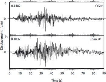
Fig. 13. Vertical displacement generated by a tectonic earthquake recorded at (a) SISMALP station OG03 and at (b) sensor 1. The maximum of displacement is indicated at the top left corner of each window in μm. For sensor 1, we computed an amplification factor of 0.698 which is almost equal to the amplification factor of OG03, 0.700.
Table 2. Tectonic earthquakes recorded at both station OG03 and our network. The three first events are used in the station-dependent coefficients calculation. The fourth event was too close, but was used in the attenuation law determination

We then scaled an attenuation law of the form of Equation (8) with our set of amplitudes and the tectonic earthquakes. This system of equations was solved by least squares, after constraining the value of M L for the tectonic earthquakes:
for station i and for tectonic event k. Δ(k
) and ![]() are given by the SISMALP catalogue and A
(i,k) is the peak-to-peak amplitude of displacement (in μm) measured by our array. This inversion leads to c = −1.2164 ± 0.0013. In order to validate this result, we processed full-waveform numerical simulations of wave propagation (Reference O’Brien and BeanO’Brien and Bean, 2004) from a few located sources to different recorders set all over the glacier, including the nine actual sensors. From these simulations, we computed the attenuation law with the following constraint on amplitude which corresponds to the magnitude 0 earthquake as defined earlier:
are given by the SISMALP catalogue and A
(i,k) is the peak-to-peak amplitude of displacement (in μm) measured by our array. This inversion leads to c = −1.2164 ± 0.0013. In order to validate this result, we processed full-waveform numerical simulations of wave propagation (Reference O’Brien and BeanO’Brien and Bean, 2004) from a few located sources to different recorders set all over the glacier, including the nine actual sensors. From these simulations, we computed the attenuation law with the following constraint on amplitude which corresponds to the magnitude 0 earthquake as defined earlier:
This numerical simulation leads to c = −1.2, which is in good agreement with our data. The constraint upon the amplitude of a reference earthquake clearly has an important weight on these results.
Once the attenuation law is determined, local magnitudes are computed for all 11 410 localized icequakes by applying Equation (7). Figure 14 shows the number of occurrences vs the magnitude. We model this magnitude–occurrence relationship by assuming that the number of earthquakes of magnitude m is of the form n(m) ∼ e−βm q(m), where e βm represents the Gutenberg–Richter law with β = b log e 10 ∼ 2.3b (the coefficient b is the b value), and q is the probability that an earthquake of magnitude m would be detected by the network. The function used in our case is of the form

which is the integral of a normal law with expected value μ and standard deviation σ. Such a form comes from the assumptions: (a) detection is hampered by the noise at the station, and (b) this noise is log-normal, as is usually observed. The maximum likelihood estimator, using Poisson statistics, yields μ = −2.26 ± 0.02, σ = 0.27 ± 0.01 and b = 0.99 ± 0.02. The magnitude of completeness can be estimated as m c = μ + σ = −1.98 ± 0.03 (Reference Ogata and KatsuraOgata and Katsura, 1993). Interestingly, the b value is very close to 1 which is a typical value for tectonic earthquakes at much larger magnitudes. This suggests that fracturing in an alpine glacier, at least within a serac zone, is at criticality with no characteristic size events dominating the process. The data follow this law for magnitudes ranging from M L = −3 to −0.15. Higher-magnitude events are serac falls, with source mechanisms different from those of type I events.

Fig. 14. Number of occurrences vs magnitude, fitted by a law taking into account the capacity of the network to detect a given event (line). The data follow a classical Gutenberg–Richter law. The black triangles show the magnitude of completeness.
9. Discussion and Conclusion
We have seen that the high seismic activity was concentrated in several clusters. We should again stress that these clusters are well determined close to the antennas. This should not rule out the possibility that there might be other clusters elsewhere in the glacier. Many different processes can be invoked to explain both the high seismic activity that we recorded and the four clusters.
The first process to consider is obviously the fall of seracs on the Rognon. Type II events are composed of many smaller events that can be explained by the fall of ice on the surface of the glacier or directly on the bedrock (at the Rognon) when the serac breaks down on the glacier (Fig. 3). As shown in Figures 9 and 10, seracs that break on the rock flow down the glacier in an avalanche of ice debris.
The second process is the opening and widening of crevasses that eventually split the glacier into blocks (seracs). Previous passive seismic experiments (Reference Neave and SavageNeave and Savage, 1970) have shown that the opening of crevasses is a seismically active process that can even mask deeper sources. An important fracturing of the ice massif occurs at the serac fall under which the measurements were made since there are strong changes in the bedrock topography as well as a high deformation rate (order-of-magnitude calculations yield a deformation rate of the order 10−3 d−1). The biggest crevasses can be seen from the surface and are likely to be responsible for some of the seismic activity (see Reference Vivian and BocquetVivian and Bocquet, 1973).
Reference Deichmann, Ansorge, Scherbaum, Aschwanden, Bernardi and GudmundssonDeichmann and others (2000) showed that deep sources could exist. Since our seismometers were recording from the bottom of the glacier, we expected to measure deep events in our experiment. Reference RobinRobin (1976) suggested that stick–slip processes could occur even for temperate glaciers. According to Reference AhlmannAhlmann (1935), a temperate glacier is defined as one in which ice at a certain depth below the surface is at the pressure-melting point. Reference Goodman, King, Millar and RobinGoodman and others (1979) showed that a sudden compression applied to a sample of ice kept close to the pressure-melting point induces a rapid cooling of that sample. Hence, if the basal ice of a temperate glacier is close to the pressure-melting point, an increase of the hydrostatic pressure will rapidly cool that parcel of ice, freezing it to the bed. Since the glacier is in motion, the accumulation of stress at this point leads to a sudden rupture of the frozen patch and to stick–slip.
Reference Goodman, King, Millar and RobinGoodman and others (1979) installed three wire strain-meters in the galleries of Glacier d’Argentière for 3 week periods in September 1975, January 1976 and April 1976. The strainmeters were installed at locations close to stations 7, 8 and 9 of our experiment. Their records showed long-period strain changes which they related to Earth tides. They recorded two types of strain events on the three data-loggers. The first type was strain excursion which begins with a rapid change followed by a slow decay back to the original value, while the second type was small offsets from the general trend. They related the first type of strain event to observations on tiltmeters set close to the San Andreas fault in California by Reference McHugh and JohnstonMcHugh and Johnston (1977). They also coupled these strain measurements with a seismometer and observed that some of the strain events were correlated with seismic events. Thirty per cent of the events were measured by at least two of their three recorders. Although these strain events could be explained by the opening of crevasses, it appeared that some of them were due to local phenomena that could be explained by the fracturing of ice frozen to the bedrock.
The clusters that we show in Figure 8 support the hypothesis of local stick–slip processes rather than the opening and widening of crevasses, since the activity is not distributed across the width of the glacier as we would expect if only crevassing were considered. One of the clusters is actually close to the site where Reference Goodman, King, Millar and RobinGoodman and others (1979) chose to install their wire strainmeters.
Similarly, Reference HubbardHubbard (2002) measured the displacement of the basal ice under Glacier de Transfleuron, Switzerland. Five anchors were placed in the ice, at different heights above the bedrock. Hubbard reported a non-uniform motion, varying both with time and with distance to the glacier bed. The total motion occurred in discrete events separated by periods of little motion, which could be explained by stick–slip.
Another possible stick–slip mechanism could be caused by the numerous rock inclusions that are found in the basal ice (Reference Vivian and BocquetVivian and Bocquet, 1973). The friction of such blocks on asperities of the bedrock could generate the seismic signals we recorded. However, we found multiplets of icequakes (two events are depicted in Figure 15a) that can be defined as a set of events with similar waveforms (Reference Got, Fréchet and KleinGot and others, 1994). These multiplets can be explained by similar source mechanisms located at the same place or close to each other.
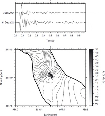
Fig. 15. (a) Two events belonging to a multiplet composed of 28 events. The lower event occurred on 11 December at 0432 h while the upper event occurred on 3 January at 0428 h. The signals were band pass-filtered between 2 and 40 Hz. Despite the very similar first arrivals, some differences are noticeable in the coda demonstrating how the medium in which the waves propagated might have changed. (b) PDF of the multiplet epicentral position with maximum corresponding to one of the patches shown in Figure 8.
Figure 15b displays the PDF averaged over the 28 events of one multiplet. It is located on one of the clusters found earlier. The time between events belonging to that cluster is sufficiently large to suggest that these sources are not moving with the glacier and that they are therefore located at the interface between the bedrock and the bottom of the glacier. The elongated form of the PDF distribution is likely to be an artefact of the array geometry. Reference Danesi, Bannister and MorelliDanesi and others (2007) found similar results beneath an Antarctic outlet glacier. This again supports the hypothesis of local basal ice freezing to the bedrock and tends to invalidate the rock-on-rock stick–slip hypothesis, which depends on both the size and shape of the rock inclusion and of bed asperities. Such a mechanism is unlikely to explain the existence of the multiplet.
In order to locate the icequake sources, we proposed an approach in which each point of the DEM is a test source from which we trace rays for several different velocity models, i.e. we work in the far-field hypothesis. Even though the sources can be very close to the sensors, both their size (according to the negative magnitudes computed in section 7) compared to the source–station distances and the DEM grid spacing (30 m) support such a hypothesis.
We then compute the PDF of the whole set of detected icequakes, providing a picture of the seismic activity over the considered period of time. This method works as long as the seismometers are close enough to record a coherent but delayed signal so that we can calculate a delay with a precision lower than the sample rate. We have seen that even in the case of small antennae, the solution found is robust as long as we have enough data (both in terms of number of events and number of antennae). Moreover, the use of probabilities gives an original approach to grid-search methods in antenna techniques. It yields both the locations of the sources via the mean value, and the error on these locations via the standard deviation of the PDF. However, it relies on the fact that there are a high number of events being processed at once.
Acknowledgements
We are grateful to Emosson S.A. for access to the galleries. We thank V. Goudard, J. Grangeon and P. Rampal for help with the fieldwork, B. Valette for numerous discussions about the inversion process, and F. Thouvenot for SISMALP data. J. Weiss, B. Hubbard, D. Chandler and an anonymous reviewer made helpful comments that significantly improved the manuscript. P.-F.R. was supported by the Conseil Général de la Région Rhône-Alpes. This work was partly funded by BQR Université de Savoie. Figures were made using the GMT package (Reference Wessel and SmithWessel and Smith, 1991).


