


INTRODUCTION
From a historical point of view, the progressive transition to farming represents a major technical, social, economic, and cultural transformation of the societies that we have now inherited. On a global scale, this “Neolithic transition” consists of a multitude of experiences, which are in turn rooted in varied temporalities. In Europe, we seek to identify the vectors of diffusion (cultural diffusion via native hunter-gatherer societies versus demic diffusion by population migrations from the Near East, where many of the domestic plant and animal species originate from), as well as the rhythms of emergence of the new Neolithic world. In this context, radiocarbon (14C) data play a major role in research focusing on modeling the speed of expansion and the spatio-temporal development of the Eurasian agricultural transition.
Since the development of the 14C method and its application to the Neolithic period between 1950 and 1960, many scenarios have been put forward. Among the founding models propounding the hypothesis of demic diffusion, we will cite those of Clark (Reference Clark1965) and Ammerman and Cavalli-Sforza (Reference Ammerman and Cavalli–Sforza1971). The first proposes to observe the diffusion of the Neolithic through the geographic dispersal of the dates, based on 73 dated sites extending from the Near East to the Atlantic and from Sub-Saharan Africa to Scandinavia. All of these dates (expressed in BCE uncalibrated) are classified into three chronological groups and their spatial distribution is plotted. Through the study of the diffusion of the Neolithic economy in space and time, J.G.D. Clark validates the classical model of dispersal from east to west established at the beginning of the 20th century based on material culture. The second model is based on a quantitative analysis of the diffusion of the agro-pastoral economy. It does not take into consideration the spatial dispersal of the radiocarbon data, but quantifies the speed of dispersal from a center of diffusion located in the Near East. The work is based on the 14C dates from 53 Neolithic sites considered to be representative of the arrival of the first farmers in different parts of Europe. The question of the link between these chronological data (expressed in BP conventional) and their spatial position is then assessed via a regressive analysis in order to describe the type of correlation observed between time and space. The result is a constant diffusion speed in time and space (1 km/year). This “wave of advance” model explains the Neolithic transition by a regular movement of populations as a result of an ever-increasing demography contributing to the segmentation of groups.
During the period from 1980 to 2000, the number of dates increased considerably. On account of this development, associated with calibration corrections, radiocarbon data are now a key tool of reflection for assessing the dynamics of European Neolithisation and the pathways it took (for example Guilaine Reference Guilaine2001; Gkiasta et al. Reference Gkiasta, Russell, Shennan and Steele2003; Pinhasi et al. Reference Pinhasi, Fort and Ammerman2005; Davison et al. Reference Davison, Dolukhanov, Sarson and Shukurov2006; Lemmen et al. 2011; Bocquet-Appel et al. Reference Bocquet-Appel, Naji, Vander Linden and Kozlowski2012). In these different works, based on varied methods of analyses, the “wave of advance” model is defined through the new corpus of dates, but also criticized by emphasizing the heterogeneity of the dynamic of expansion.
In the Western Mediterranean, it is now well known that the first agro-pastoral economy appears around 6000 BCE in southeastern Italy and that all of the sites, often grouped under the generic term “Impressed Ware” (as they are characterized by pottery decorated with impressions made by varied implements), represent the departure point for the dispersal of the Neolithic economy. Within this area, different cultural groups (Impressa, Cardial, Epicardial) are distinguished according to their technical productions and their economical resources (Guilaine and Manen Reference Guilaine and Manen2007). Predictably, the different works addressing this question grant considerable importance to maritime colonization models and again, radiocarbon dates form the basis of these demonstrations. The analysis of audited database underlines the low chronological gap between the emergence of the Neolithic economy in the center of Italy and Portugal, or between the Gulf of Lion and Portugal (Binder and Guilaine Reference Binder and Guilaine1999; Zilhão Reference Zilhão2001; Manen and Sabatier Reference Manen and Sabatier2003; Bernabeu Aubán Reference Bernabeu Aubán2006; Manen Reference Manen2014; Bernabeu Aubán et al. Reference Bernabeu Aubán, Barton, Pardo Gordó and Bergin2015; Martins et al. Reference Martins, Oms Arias, Pereira, Pike, Rowsell and Zilhão2015; Binder et al. Reference Binder, Angeli, Gomart, Guilaine, Manen, Maggi, Muntoni, Panelli, Radi, Tozzi, Arobba, Battentier, Brandaglia, Bouby, Briois, Carré, Delhon, Gourichon, Marinval, Nisbet, Rossi, Rowley-Conwy and Thiébault2017; Isern et al. Reference Isern Sardó, Zilhao, Fort and Ammerman2017). This rapid dispersal is then interpreted as part of a pioneering colonization model based on the use of maritime routes, associated by some authors with leapfrog colonization (Zilhão Reference Zilhão1993; Binder Reference Binder2013). These data, like those obtained in continental Europe (Boguki Reference Bogucki2000 for example), overturn the “wave of advance” model in favor of a model of arrhythmic diffusion (Guilaine Reference Guilaine2013).
The establishment of a reliable chronological framework is thus a fundamental prerequisite for understanding the mechanisms of Neolithisation. In this article, we discuss the emergence dynamics of the Neolithic in the Western Mediterranean based on a renewed corpus of dates taken as part of the “PROCOMEFootnote 1 – Continental extensions of Mediterranean Neolithisation” research program, financed by the French National Agency of Research. In this programme, more than a hundred new AMS dates were obtained on samples selected following a specific protocol. Here, we present a selection of these results, which are discussed in the general context of the Neolithic transition in the Western Mediterranean. Our contribution consists of three main points:
∙ As classically observed in many works, the speed of diffusion of the Neolithic economy is very fast in the Western Mediterranean and probably underlines the role of the sea as a fundamental vector. Indeed, the earliest traces of the agro-pastoral economy in the South of France are dated between 5800 and 5600 cal BCEFootnote 2 . These dates were obtained from charred cereal seeds from the coastal sites of the Hérault department. They show how early the Neolithic impacted the South of France, probably in connection with the maritime movements of pioneering groups, at the very beginning of the 6th millennium BCE.
∙ However, the comparison of these results with those obtained in Italy and in Spain refutes the hypothesis of a steady progression along the coast. Indeed, in the light of current data, the spatial distribution of technical and economic Neolithic innovations from the south of Italy is not strictly correlated to the time factor and thus reflections on the dispersal mechanisms operating in this Mediterranean area require further consideration.
∙ In a later phase, after these first Neolithic impacts, the diffusion rhythm of the Neolithic economy varies considerably within the Western Mediterranean zone. The variety of social and environmental contexts involved in this process undoubtedly generated diverse situations, which back up the arrhythmic model.
MATERIAL AND METHODS
Geographic Setting and Archaeological Context
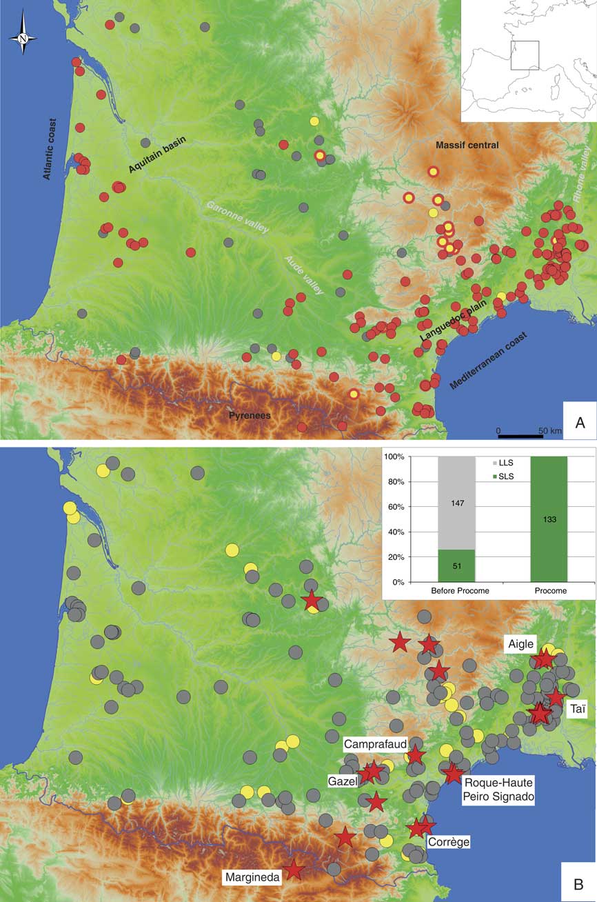
The southwest of France (Figure 1) presents several advantages for assessing Neolithisation issues. Indeed, Neolithic technical and economic innovations develop there at an early stage and in a polymorphic way, from a cultural, temporal and spatial point of view (Guilaine et al. Reference Guilaine, Manen and Vigne2007). This research window also offers the advantage of presenting major ecological contrasts: Mediterranean and Atlantic coastlines, the waterway routes of the Rhône, Aude or Garonne, the plains of the Rhone and Languedoc and the Aquitaine dune systems, the foothills of the Pyrenees and the Massif Central. Several hundred disparate sites have been recorded in this zone as a result of a long tradition of research on Neolithisation initiated in the 1960s. This study tests different hypotheses developed on a European scale by analysing the respective weight of environmental, demographic (demic diffusion) and social (cultural diffusion through borrowing) variables at these sites in the diffusion and evolution processes of the first Neolithic societies.
Geographic setting of the studied area and location of the archaeological sites related to the Neolithic transition. A: yellow circle: Late Mesolithic; yed circle: Early Neolithic; yellow circle with a red border: Late Mesolithic and Early Neolithic; gray circle: uncertain attribution. Map B: yellow circle: sites with 14C-dates; grey circle: undated sites; red star: sites dated in the framework of the Procome project; the named sites are those discussed in this paper. The histograms show on the left the dataset of radiocarbon dates available before the Procome project and on the right the dataset of radiocarbon dates of the Procome project (SLS: short-lived sample; LLS: long-lived sample).
Site Selection
The selection strategy for the sites to be dated is based on a critical documentary overview (Perrin et al. Reference Perrin, Manen, Valdeyron and Guilaine2017) of the 244 sites attributed to the Second Mesolithic, on the basis of the technical systems (i.e., techno-complex of blades and trapezes, Perrin et al. Reference Perrin, Marchand, Allard, Binder, Collina, Garcia Puchol and Valdeyron2009), and the Early Neolithic (Manen Reference Manen2014). Among these, 45 sites (or 18%) had already been dated, for a total of 198 measurements ranging from the end of the 7th millennium to the beginning of the 5th millennium BCE (Figure 1). After a critical examination of the archaeological link (Manen and Sabatier Reference Manen and Sabatier2003; Zilhão Reference Zilhão2011) of each of these 198 measurements, it was only possible to retain 156 dates (20% of the results were considered as poor reliability), three-fourths of which were taken on long-lived samples (mainly charcoal). Considering this outcome and the problems mentioned above, 24 key sites were selected in order to obtain a high-precision chronological framework. The new AMS dates come from sites with varied characteristics and are distributed between the coastal zone and the Mediterranean hinterland. Some of them present a long stratigraphy whereas others present an insight into a much narrower time frame of the Neolithic transition. Prior to this, most of these sites underwent a detailed chrono-stratigraphic critical evaluation (geoarchaeological analyses, lithic and ceramic refits…) in order to ensure that the dating samples were as reliable as possible.
Sample Selection and AMS 14C Dating
In order to guarantee the relevance and the reliability of the results, a precise protocol was established for sample selection. It is based on two main criteria: the “nature” of the radiocarbon event and its “link” with the human event that we wish to date. The notion of radiocarbon event was defined by Van Strydonck et al. (Reference Van Strydonck, Nelson, Crombé, Bronk Ramsey, Scott, Van der Plicht, Hedges and Evin1999) and signifies “the isolation of some carbon-containing substance from the reservoir(s) from which its carbon was obtained. In colloquial terms, the 14C event starts the radiocarbon clock”. This radiocarbon event, which can be of very variable duration, is determined by the intrinsic characteristics of the sample (seed versus old tree). Thus, in order to ensure that the delta between the real age and the measured age is as low as possible (Waterbolk Reference Waterbolk1971; Wood Reference Wood2015), we selected first and foremost samples with a short life cycle: charred seeds, unburnt animal bones. As for the archaeological link, it estimates the degree of archaeological representativeness of the date (the taphonomy of Bayliss Reference Bayliss1999 “the relationship between the material dated and the context from which it was recovered”). This is measured in relation to the archaeological criteria and is thus based on the extrinsic characteristics of the dated sample. We were thus particularly attentive to the reliability of the archaeological contexts from which the samples were taken. For the issues concerned here, we privileged sites with a well-know taphonomic history (Guilaine Reference Guilaine1993; Bernabeu Aubán et al. Reference Bernabeu Aubán, Barton and Perez Ripoll2001; Zilhão Reference Zilhão2011) and samples coming from an anthropogenic structure (pit, hearth…), bones from a consumed faunal accumulation, samples with a direct link with the occupation to be dated: domestic taxa, bone tools… On average, four dates were made at single-phase sites in order to test the homogeneity of the series. For stratified sites, we dated between 10 and 15 samples covering the whole range of the stratigraphy.
Concerning the animal bones, the different samples for a site, or for a layer in the case of stratified sites, correspond insofar as is possible to distinct individuals (Minimum Number of Individuals). Taxonomic identification or reexamination conducted for this project is based on morphological (for Caprini: Boessneck et al. Reference Boessneck, Müller and Teichert1964; Helmer Reference Helmer2000; Fernandez Reference Fernandez2001; Halstead et al. Reference Halstead, Collins and Isaakidou2002; Zeder and Pilaar Reference Zeder and Pilaar2010; Gillis et al. Reference Gillis, Chaix and Vigne2011; Mallet and Guadelli Reference Mallet and Guadelli2013) and metrical criteria (for Bos sp.: Degerbol and Fredskild Reference Degerbøl and Fredskild1970; Helmer and Monchot Reference Helmer and Monchot2006; Scheu et al. Reference Scheu, Hartz, Schmolcke, Tresset, Burger and Bollongino2008). The choice of the taxa sampled was closely related to issues peculiar to each archaeological site. However, at least two domestic specimens were sampled at each site.
Charred seeds have been selected from samples currently under study (Taï) or from samples that have been studied previously (Balma Margineda, Pont de Roque-Haute, Peiro Signado). In all cases, these samples have been reassessed with a stereomicroscope and their identification has been validated using the current morphological criteria (Cappers et al. Reference Cappers and Jans2006; Jacomet Reference Jacomet2006). Cereal caryopses (domestic and cultivated plants introduced by the Neolithic community) have been favored.
Most of the 14C dating was carried out at Beta Analytic laboratory (AMS-standard delivery) using their standard pre-treatment techniques: for charred seed, the acid-alkali-acid method; for bone collagen the Longin method (extraction with alkali and additional pre-treatment with sodium hydroxide (NaOH) to ensure the absence of secondary organic acids). Reported results are accredited to ISO/IEC 17025:2005 Testing Accreditation PJLA #59423. The reported δ13C values were measured separately in an IRMS (isotope ratio mass spectrometer). They are not the AMS δ13C, which would include fractionation effects from natural, chemistry and AMS induced sources standards.
Calibration and Statistics
Calibration and sample significance tests were carried out with OxCal 4.2 using the IntCal13 curve (Table 1; Stuiver and Reimer Reference Stuiver and Reimer1993; Reimer et al. Reference Reimer, Bard, Bayliss, Beck, Blackwell, Ramsey, Buck, Cheng, Edwards, Friedrich, Grootes, Guilderson, Haflidason, Hajdas, Hatté, Heaton, Hoffmann, Hogg, Hughen, Kaiser, Kromer, Manning, Niu, Reimer, Richards, Scott, Southon, Staff, Turney and van der Plicht2013). Chronological modeling using Bayesian statistics was performed with ChronoModel, a newly available Bayesian age-modeling software (Lanos et al. Reference Lanos, Philippe, Lanos and Dufresne2015; Lanos and Philippe Reference Lanos and Philippe2017, Reference Lanos and Philippe2018).
Set of the 14C dates obtained from eight settlements in the southwest of France and discussed in this paper. Calibration is with OxCal 4.2 using IntCal13 (Reimer et al. Reference Reimer, Bard, Bayliss, Beck, Blackwell, Ramsey, Buck, Cheng, Edwards, Friedrich, Grootes, Guilderson, Haflidason, Hajdas, Hatté, Heaton, Hoffmann, Hogg, Hughen, Kaiser, Kromer, Manning, Niu, Reimer, Richards, Scott, Southon, Staff, Turney and van der Plicht2013). Criteria for evaluating the poor reliability of some dates are explained in the column “Comment on the result”: 1: Long-lived material and large standard deviation; 2: Too young for industry; 3: Laboratory physico-chemical results unacceptable. Full data are available in the supplementary material.
The essential characteristics and the main operating principles of this software have been well summed up in a recent paper (Binder et al. Reference Binder, Angeli, Gomart, Guilaine, Manen, Maggi, Muntoni, Panelli, Radi, Tozzi, Arobba, Battentier, Brandaglia, Bouby, Briois, Carré, Delhon, Gourichon, Marinval, Nisbet, Rossi, Rowley-Conwy and Thiébault2017). One of its main points is that it is based “on the Bayesian event date model, which is aimed at estimating the date of a target event from the combination of individual dates derived from relevant dated events” (Binder et al. Reference Binder, Angeli, Gomart, Guilaine, Manen, Maggi, Muntoni, Panelli, Radi, Tozzi, Arobba, Battentier, Brandaglia, Bouby, Briois, Carré, Delhon, Gourichon, Marinval, Nisbet, Rossi, Rowley-Conwy and Thiébault2017: 57). Since the target dates are modeled through their individual variance, the models constructed are not very sensitive to several kinds of errors, and especially to outliers (Lanos and Philippe Reference Lanos and Philippe2018). “Thanks to this modeling, it is not necessary to discard outliers because the posterior (in the Bayesian sense) high values of the individual variances will automatically penalise their contributions to the estimate of event date” (Binder et al. Reference Binder, Angeli, Gomart, Guilaine, Manen, Maggi, Muntoni, Panelli, Radi, Tozzi, Arobba, Battentier, Brandaglia, Bouby, Briois, Carré, Delhon, Gourichon, Marinval, Nisbet, Rossi, Rowley-Conwy and Thiébault2017: 57). Each modeling uses a model of events in which are placed the stratigraphic constraints really observed in the field. A phase model can also be constructed, each phase including a number of target dates, in order to test interpretative hypotheses.
In this work, we performed for every model three runs of Monte Carlo Markov’s Chains of 100.000 iterations each. The beginning, the end and the duration of all the phases are then estimated. The values retained are those of the modes a posteriori (MAP) and those of the Highest Posterior Density regions (HPD) at 95% probability. These two values are calculated for the beginning (B_MAP and B_HPD hereafter) and the end (E_MAP and E_HPD hereafter) of each phase. For phases that contain multiple target dates, it is also possible to estimate the duration (D_HPD, at 95% probability too). The graphic outputs retranscribe the HPD regions of beginning and end of phases as two density curves, the oldest being the beginning, the most recent the end.
RESULTS
Some of these new results, in particular those linked to the last Mesolithic events and the Neolithisation of the hinterland, were published in Perrin et al. (Reference Perrin, Manen, Valdeyron and Guilaine2017), and here we have chosen to present 76 dates (45 new ones from our projects and others from the literature), partly unpublished, from eight key sites (Figure 1 and Table 1) from the coastal region, allowing for a new reading of the main issues of the Neolithic transition.
Grotte de l’Aigle
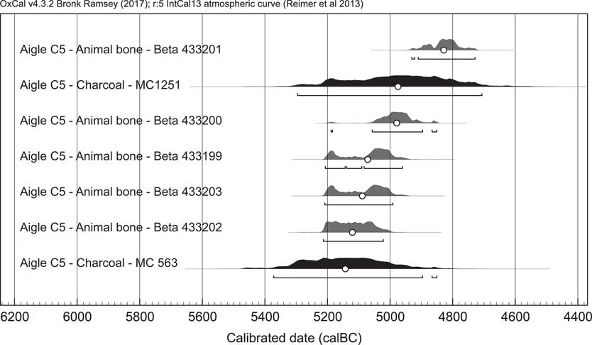
This cave is located in the Gard department (Figure 1), opens out onto a rocky spur forming the northern side of a vast limestone plateau limited by the Cèze valley, to the north and the east, and the Ales basin to the west. It comprises a vast entrance (10 m wide and 10 m high), leading into a relatively low chamber. It was excavated by Roudil in the 1970s (Roudil et al. Reference Roudil, Roudil and Soulier1979) and contained a stratigraphy extending from the Early Neolithic to the Bronze Age. The excavations extended over the whole chamber, representing a surface of nearly 20 m2, and attained a depth of approximately 1.50 m. The Early Neolithic comes from layer 5 (c.5) and consists of objects with all the characteristics of the Cardial (pottery decorated with horizontal bands often with a border and formed by impressions made with a Cardium shell, blade debitage on flint, transverse arrowheads). The faunal assemblage, re-examined in the framework of the Procome project, consists mainly of Sus remains. The status, wild or domestic, of these animals remains unclear. On the other hand, Bos and Caprini bones can be reliably assigned to domestic cattle, sheep and goat. Several cereal remains (soft wheat) are also mentioned in the 1979 publication. In the 1970s, the only two 14C dates carried out at the site were obtained from charcoal from this c.5 layer. These two dates presented a chronological discrepancy (Manen and Sabatier Reference Manen and Sabatier2003). All of the remains from layer 5 were reviewed as part of the PROCOME program. As this excavation was carried out during the 1970s and was partly published, we have no information to test the depositional integrity. Our sample selection was guided by the location of the remains (the square selected provides a high artifacts density and this assemblage looks homogenous and very coherent) and by a new study of the faunal remains using the latest methods. By this way, we selected five samples, of which two have been assigned to domestic cattle and sheep, attributed by the excavators to layer c.5. The aim was to define the chronological position of this layer and to enhance the chronology of the Cardial (Table 1; Figure 2). Apart from Beta-433201, the new measurements are statistically identical (χ2=5.6, df=5, α[5%]=11.1). These four dates combined place the occupation of the site between 5200 and 4990 cal BCE. The fifth date (Beta-433201) presents a slight chronological discrepancy, which could suggest a more recent occupation. However, none of the objects confirm this hypothesis. All the values are good (C:N %C, %N), which supports the historical proxies. The procedures of analysis and consideration of good collagen for analysis were identical in all cases. The available archaeological and stratigraphic data thus either point towards a single occupation, or to several occupations over a very short interval of time. Two Bayesian models can thus be constructed on the basis of these two hypotheses (Figure 3). If we consider that all the available dates relate to a single occupation, we can construct a very simple model where all the measurements are related to the same event (including the Monaco dates-MC), forming the only dated occupation phase for the site. In this case, layer 5 of grotte de l’Aigle would be dated between 5110 and 4950 cal BCE (highest posterior density region or HPD region [95%]) with a maximum a posteriori (or MAP) at 5030 cal BCE (Table 2). If we consider that all the dates obtained are potentially related to as many short occupations but that we cannot periodize them due to the lack of micro-stratigraphic data, then we can construct a second model where the seven available dates are related to as many separate events, but are included in the same phase. In this second case, the ranges obtained are clearly more spread out. The beginning of the layer 5 occupations would thus be situated at about 5210 cal BCE (MAP value; HPD region: 5670–5040 cal BCE [95%]), whereas the end of these occupations would occur towards 4810 cal BCE (Table 2; MAP value; HPD region: 4980–4380 cal BCE [95%]). Both models thus present convergent results, which are less precise in the second case. This excavation was carried out during the 1970s and unfortunately, it is not possible to objectively choose between these two results. We can thus only conclude that the layer 5 occupations from grotte de l’Aigle are probably situated between 5210 and 4810 cal BCE, and maybe more specifically between 5110 and 4950 cal BCE.
Calibrated probability distribution of radiocarbon dates from la grotte de l’Aigle c.5. OxCal v 4.3.2 Bronk Ramsey (Reference Bronk Ramsey2017); r:5 and IntCal13 atmospheric curve (Reimer et al. Reference Reimer, Bard, Bayliss, Beck, Blackwell, Ramsey, Buck, Cheng, Edwards, Friedrich, Grootes, Guilderson, Haflidason, Hajdas, Hatté, Heaton, Hoffmann, Hogg, Hughen, Kaiser, Kromer, Manning, Niu, Reimer, Richards, Scott, Southon, Staff, Turney and van der Plicht2013). In gray, short-lived samples and dates obtained by AMS; in black, conventional methods of radiocarbon dating on long-lived samples.
The two Bayesian models of the Aigle Cave (events on the left part of each diagram, phases on the right; ChronoModel 2.0.4). At the bottom, posterior density distribution of each model. As there is only one event in the model A, it is not possible to calculate the beginning and the end of the phase. For the Model B, the density region of the beginning is the oldest. The areas below the curves represent the 95% highest posterior densities.
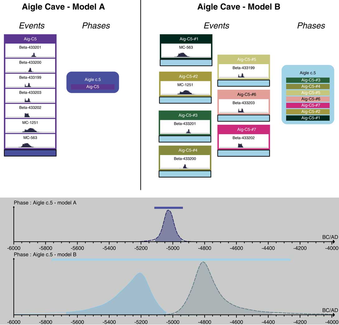
At the top: modeled events of the Aigle cave. The number of associated dates is for each event indicated in brackets; e_HPD (95%), i.e. event’s highest posterior density interval at 95% confidence; e_MAP, event’s posterior mode. At the bottom: modeled phases of the Aigle cave. The number of associated events and dates for each event is indicated in brackets: D_HPD (95%), highest posterior density interval at 95% confidence of phase duration; D_MAP, posterior mode of phase duration; B_HPD (95%), highest posterior density interval at 95% confidence of phase beginning; B_MAP, posterior mode of phase beginning; E_HPD (95%), highest posterior density interval at 95% confidence of phase’s end; E_MAP, posterior mode of phase’s end. For the Model A, as there is only one event in the phase, it is not possible to calculate a duration, nor to distinguish a beginning and an end of phase.

Balma Margineda
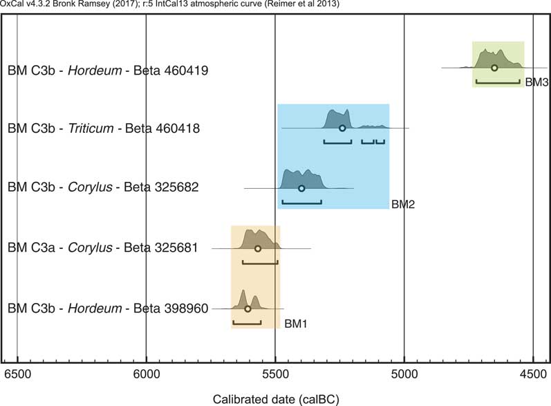
The Balma Margineda rock shelter, in Andorra, opens near the bottom of a slope, in a schist massif at an altitude of 945 m (Figure 1). The site was excavated by Guilaine between 1979 and 1991 (Guilaine and Martzluff Reference Guilaine and Martzluff1995). A very long sedimentary sequence was identified over a depth of 3.50 m, recording a succession of Azilian, Mesolithic, Early Neolithic occupations, as well as remains from historical periods. The Early Neolithic occupations were observed in layer 3 (c.3), which presents sedimentary variations and several anthropogenic structures (pits and hearths), making the overall stratigraphic reading more complex (Oms et al. Reference Oms Arias, Gibaja Bao, Mazzuco and Guilaine2016). For this reason, layer 3 was internally subdivided. This layer yielded diversified, but relatively sparse objects. Among the pottery, 53 impressed vases decorated with diverse patterns, including shell impressions, incisions, grooves and the addition of modeled decorations were identified. Although theses vases are not totally representative of a specific facies, they clearly belong to the Impressed ware. Among the lithic industry several chaînes opératoires are identifiable according to the raw materials used (metamorphic rocks, quartz, rock crystal, and flint). It seems that some of the débitage did not take place at the site. Retouched elements are rare and only 18 geometric arrowheads were found at the excavation. The carpological and archaeozoological analyses identified the consumption of cereals, pulses and domestic sheep and goats. However, hunting and gathering also provided food resources. On account of its geographic position in the heart of the Pyrenees, the Balma Margineda Neolithic sequence is at the center of many debates relating to the early impact of the Neolithic in mountainous zones and the emergence of the Neolithic in Spain. Balma Margineda is effectively considered by some authors as a milestone in the progression of the Neolithic economy towards the Aragon region (Utrilla and Domingo Reference Utrilla Miranda and Domingo Martinez2014). These discussions are summarized in two recent articles (Martins et al. Reference Martins, Oms Arias, Pereira, Pike, Rowsell and Zilhão2015; Oms et al. Reference Oms Arias, Gibaja Bao, Mazzuco and Guilaine2016). Since the end of the excavation, 15 dates have been made on layer 3 (Table 1). These dates result from different research programmes. A first batch was undertaken at the end of the1980s, in the Lyon laboratory, on charcoal. These dates all present high standard deviations (Ly-2839, Ly-3288 to Ly-3290). On the other hand, they are relatively stratigraphically consistent. These results date layer 3 to between 6000 and 5500 cal BCE. In recent work focusing on the question of the emergence of the agro-pastoral economy in Spain, two new dates were carried out (Martins et al. Reference Martins, Oms Arias, Pereira, Pike, Rowsell and Zilhão2015; Beta-325681 and Beta-325682). This time, short-lived samples were selected: hazelnuts (Corylus avelana) from layers C3b and C3a. Both of the measurements obtained are statistically very different (χ2=15.1, df=1, α[5%]=3.8) and present a stratigraphic inversion. In this way, according to the authors “none of the Margineda samples so far dated, including our own, can be securely related to the material culture found alongside them in layer 3” (Martins et al. Reference Martins, Oms Arias, Pereira, Pike, Rowsell and Zilhão2015). Lastly, a third research programme focusing on the first communities in the northeast of Spain gave rise to new dates on short-lived samples in the Seville laboratory (bones from wild and domestic animals) from layer 3 (Oms et al. Reference Oms Arias, Gibaja Bao, Mazzuco and Guilaine2016). But these four dates yielded incoherent δC13 values, pointing to a physico-chemical contamination of the sample. As part of the PROCOME project, we decided to date only the charred cereal seeds retrieved from the flotation of sediments from layer 3 (Marinval Reference Marinval1995). Indeed, the only way to counter the problem of the post-depositional processes was the direct radiocarbon dating of domestic specimens (Martins et al. Reference Martins, Oms Arias, Pereira, Pike, Rowsell and Zilhão2015). Five samples were selected: barley (Hordeum vulgare), naked wheat (Triticum aestivum/turgidum) and emmer (Triticum dicoccum). Two of these charred seeds are intrusive in layer 3, as they gave measurements attributable to the Iron Age (Beta-398959 and Beta-460420). Again, these results underline the complexity of the stratigraphy of Balma Margineda and the post-depositional problems. The three other measurements (Beta-398960, Beta-460418, and Beta-460419) are very different from each other, but are acceptable for the Neolithisation context. Finally, of all the dates done, we retain the 5 made on short-lived species which are compatible with the Neolithic chronology (Figure 4). However, these dates seem to be distributed in a random way in layer 3, and do not allow for the construction of Bayesian modeling. If we leave the purely stratigraphic aspects aside and only consider the dates themselves, we observe that they are clustered into three distinct groups, indicating different moments of human presence at the site (charred seeds and fruits; bones from consumed animals). A first moment (BM1, between 5635 and 5550 cal BCE) is indicated by the statistically identical Beta-398960 and Beta-325681 measurements (χ2=1.22, df=1, α[5%]=3.8). Then two other measurements are discontinuously dispersed between 5475 and 5075 cal BCE (BM2; Beta-325682 and Beta-460418). A single reliable measurement (Beta-460419) points to the frequentation of the site between 4700 and 4500 cal BCE. The site of Balma Margineda presents undeniable post-depositional problems linked to a complex stratigraphy formed by the accretion of small sedimentary units (Brochier Reference Brochier1995). As a result, it is difficult to link these three series to specific technical and economic complexes. If we retain the BM1 range, for which one of the dates is obtained on a cereal seed, the regional data (in the South of France and in Spain) pointing to the presence of Neolithic communities at this time are very rare. These dates would thus indicate a very early occupation/frequentation of mountainous environments. The BM2 series is part of the classical range of the Cardial/Epicardial sequence and shows that Balma Margineda is not outside the cultural coastline dynamics. The BM3 series indicates persisting discontinuous use of the site during the transition with the Middle Neolithic.
Calibrated probability distribution of the radiocarbon dates from Balma Margineda c3. OxCal v 4.3.2 Bronk Ramsey (Reference Bronk Ramsey2017); r:5 and IntCal13 atmospheric curve (Reimer et al. Reference Reimer, Bard, Bayliss, Beck, Blackwell, Ramsey, Buck, Cheng, Edwards, Friedrich, Grootes, Guilderson, Haflidason, Hajdas, Hatté, Heaton, Hoffmann, Hogg, Hughen, Kaiser, Kromer, Manning, Niu, Reimer, Richards, Scott, Southon, Staff, Turney and van der Plicht2013). These seven retained dates are on short-lived samples (domestic seeds and wild fruits).
Camprafaud
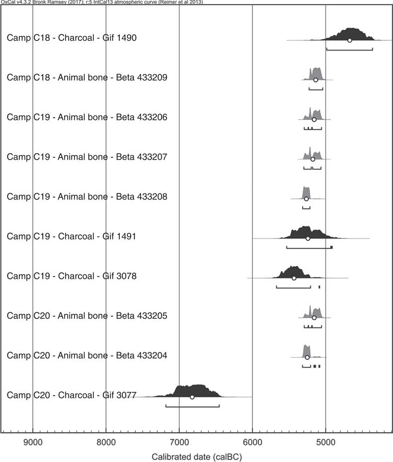
Camprafaud Cave is situated at an altitude of 441 m in the last foothills of the eastern Montagne Noire, on the southern slope of a rocky spur on the extreme west of the Pardailhan Mountains, overlooking the plain of Saint-Chinian (Figure 1). The cave consists of a chamber about 15 m deep with a maximum width of 14 m. The site was excavated during the 19th century, and again before the Second World War. Systematic excavations were then carried out by Rodriguez between 1967 and 1973. This is one of the most complete stratigraphic sequences in the Hérault, comprising occupations ranging from the Early Neolithic to the Bell Beaker culture, between the 6th and the 2nd millennia BCE. The Early Neolithic horizon was divided into five archaeological layers c.20 to c.16, of variable thickness and with different sedimentary characteristics. The material productions associated with these layers are relatively diversified, with abundant pottery. The technical and stylistic characteristics of the pottery productions and the lithic industries are related to the Cardial/Epicardial complex. These layers also contained a large faunal accumulation, indicating hunting activities and the presence of domestic animals. Here, we will focus on the layers from the base of the stratigraphy (c.20, c.19, and c.18). After the 1960–1970 excavations, 4 dates were made on unspecified charcoals (Gif-1490, Gif-1491, Gif-3077, and Gif-3078). These dates all present a very high standard deviation, and therefore they are not very relevant. As this excavation was carried out during the 1970s, we have no information to make a chrono-stratigraphic critical evaluation. Our sample selection was guided by the location of the remains (the square selected provides a high artifacts density and this assemblage looks homogenous and very coherent) and by a new study of the faunal remains using the latest methods. A new series of six samples was selected (Table 1 and Figure 5): two domestic sheep have been sampled for the level c.20 while Bos bones, from both domestic and wild cattle, have been selected for the levels c.19 and c.18. All of the formerly or recently dated samples only bear a reference to the layer, with no further detail. It is thus only possible to construct a very simple Bayesian model, where all the dates of the same layer are included in the same event (Figure 6). The stratigraphic sequence of the three layers considered is included in the phase model. The modeling shows that the occupations of these levels took place within a short time frame, during the last centuries of the sixth millennium (Table 3). Layer 20 is dated to around 5270 cal BCE (MAP value; HPD region: 5370–5180 cal BCE [95%]), layer 19 to around 5230 cal BCE (MAP value; HPD region: 5300–5120 cal BCE [95%]) and layer 18 to around 5080 cal BCE (MAP value; HPD region: 5230–4630 cal BCE [95%]).
Calibrated probability distribution of radiocarbon dates from Camprafaud c20-c18. OxCal v 4.3.2 Bronk Ramsey (Reference Bronk Ramsey2017); r:5 and IntCal13 atmospheric curve (Reimer et al. Reference Reimer, Bard, Bayliss, Beck, Blackwell, Ramsey, Buck, Cheng, Edwards, Friedrich, Grootes, Guilderson, Haflidason, Hajdas, Hatté, Heaton, Hoffmann, Hogg, Hughen, Kaiser, Kromer, Manning, Niu, Reimer, Richards, Scott, Southon, Staff, Turney and van der Plicht2013). In gray, short-lived samples and dates obtained by AMS; in black, conventional methods of radiocarbon dating on long-lived samples.
Bayesian model of the Camprafaud Cave (events on the left part of the diagram, phases on the right; ChronoModel 2.0.4). At the bottom, posterior density distribution of the model. The areas below the curves represent the 95% highest posterior densities. Arrows indicate the stratigraphic constraints applied to the successive phases.
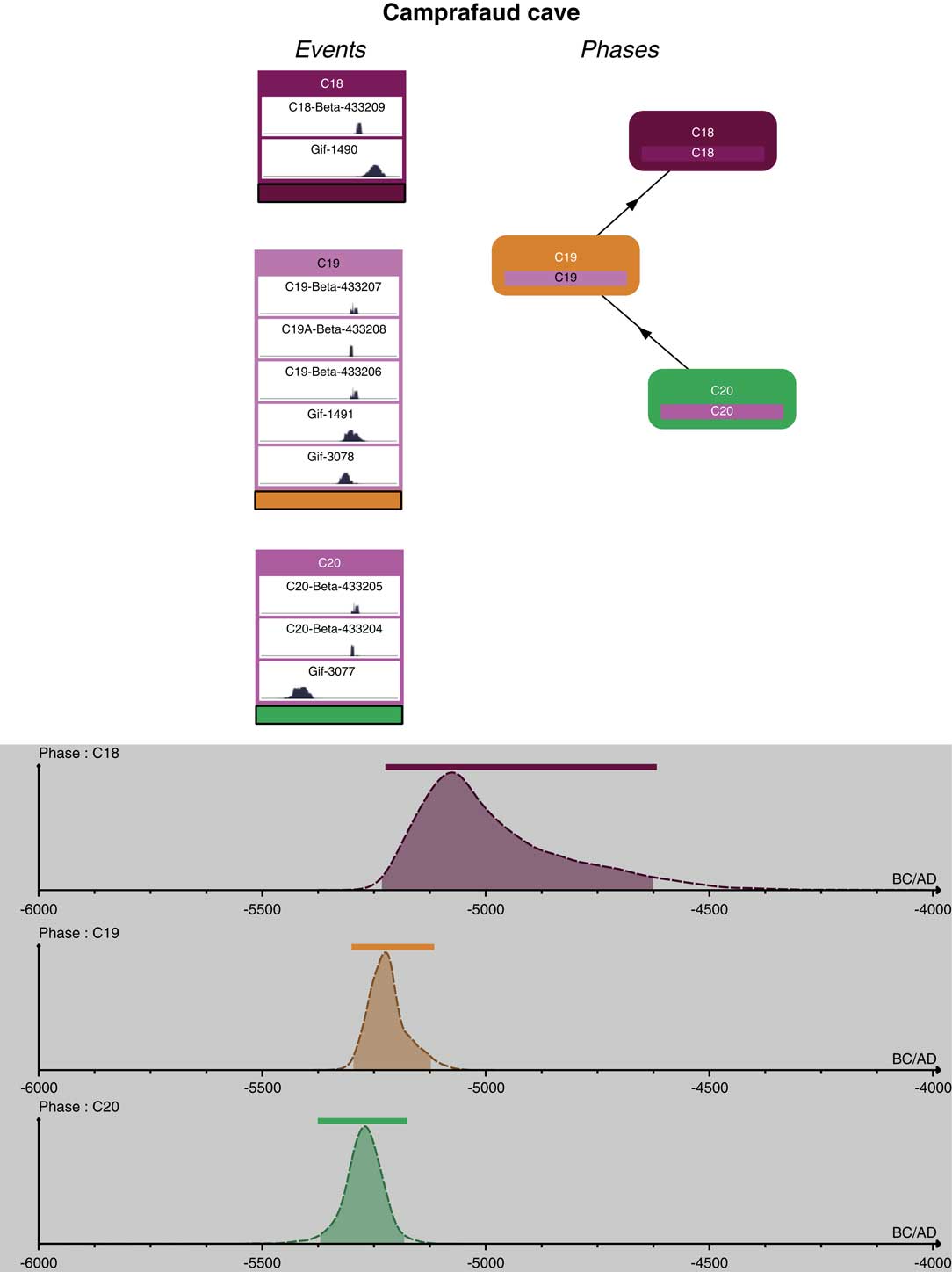
At the top: modeled events of the Camprafaud cave. The number of associated dates is for each event indicated in brackets; e_HPD (95%), i.e. event’s highest posterior density interval at 95% confidence; e_MAP, event’s posterior mode. At the bottom: modeled phases of the Camprafaud cave. The number of associated events and dates for each event is indicated in brackets: D_HPD (95%), highest posterior density interval at 95% confidence of phase duration; D_MAP, posterior mode of phase duration; B_HPD (95%), highest posterior density interval at 95% confidence of phase beginning; B_MAP, posterior mode of phase beginning; E_HPD (95%), highest posterior density interval at 95% confidence of phase’s end; E_MAP, posterior mode of phase’s end. As there are only one event in each phases, it is not possible to calculate durations, nor to distinguish beginnings and ends of these phases.
These new dates enable us to show that:
∙ The early date of layer 20 (Gif-3077) in definitively invalidated;
∙ Generally speaking, there is significant discordance between the dates on charcoal and the dates on short-lived samples, regardless of the layers. These new dates show the importance of redating sequences by focusing on short-lived samples and obtaining measurements with low standard deviations.
∙ They enable us to narrow the sequence of the first occupations of the cave (c.20 to c.18) to between about 5280 and 5070 cal BCE. We must underline the high radiometric homogeneity of these new measurements that now provide a reference for the Epicardial culture.
Gazel
Gazel Cave is located in the Montagne Noire at Sallèles-Cabardès in the Aude, at an altitude of 250 m on the left bank of the Ceize River (Figure 1). The Holocene levels were excavated by Guilaine between 1963 and 1967. The archaeological occupations are spread over different sectors of the cave called “Porche (Entrance)”, “Éboulis (Scree)” and “Salle centrale (Central Chamber)”. In the Entrance and Scree sectors, a continuous sequence between the Mesolithic and the Neolithic was identified. This site has been the object of a detailed chrono-stratigraphic critical evaluation (geoarchaeological analyses by Brochier Reference Brochier1978, lithic and ceramic refits by Briois Reference Briois2005 and Manen Reference Manen2002). During the excavation, sheep remains were discovered in the Mesolithic levels, leading to widespread discussions on the role played by the last populations of Mesolithic hunter-gatherers in the process of emergence of the Neolithic economy (for an overview, see Guilaine Reference Guilaine1993; Geddès Reference Geddès1993). Since then, these hypotheses have been discarded but these bones had never undergone archaeozoological or chronological reassessment. Therefore, we selected five samples of Ovis aries discovered in the Mesolithic levels from the “Entrance” and “Scree” sectors. For this selection, a careful re-examination of the Caprini remains has been essential as we showed that, in addition to Ovis and Capra, Rupicapra was present in the mesolithic levels of the “Scree” sectors. This third genus had not been identified in the previous study and a few bones assigned to Ovis turned out to be Rupicapra. Predictably, these five samples yielded recent dates placing them at the end of the Early Neolithic and the Middle Neolithic (Table 1). Like for several other Western Mediterranean sites (Bernabeu Aubán et al. Reference Bernabeu Aubán, Barton and Perez Ripoll2001), these new dates thus confirm that the domestic Caprini remains were reworked into horizons from the end of the Mesolithic and rule out any discussion on any potential early interactions between hunter-gatherers and Neolithic farmers.
La Corrège
The site of la Corrège, in Leucate in the Aude, corresponds to an open-air site immersed below 5 to 6 meters of water, in the Leucate-Barcarès lagoon (Figure 1). It is one of the first sites in the South of France to clearly show the impact of the rise in sea level at the beginning of the Holocene on the conservation of Neolithic sites. The site was identified in 1972 following deepening dredging work as part of the development of Port-Leucate. The dredged material was systematically sorted and diving operations were set up to try to locate the site. Abundant objects were found, particularly pottery. But, it was also possible to gather a major series of bone tools, macro-tools related to fishing activities, polished stone, fauna… Although this series is decontextualized, it nonetheless represents the most significant Cardial assemblage in Languedoc (Guilaine et al. Reference Guilaine, Freises and Montjardin1984).
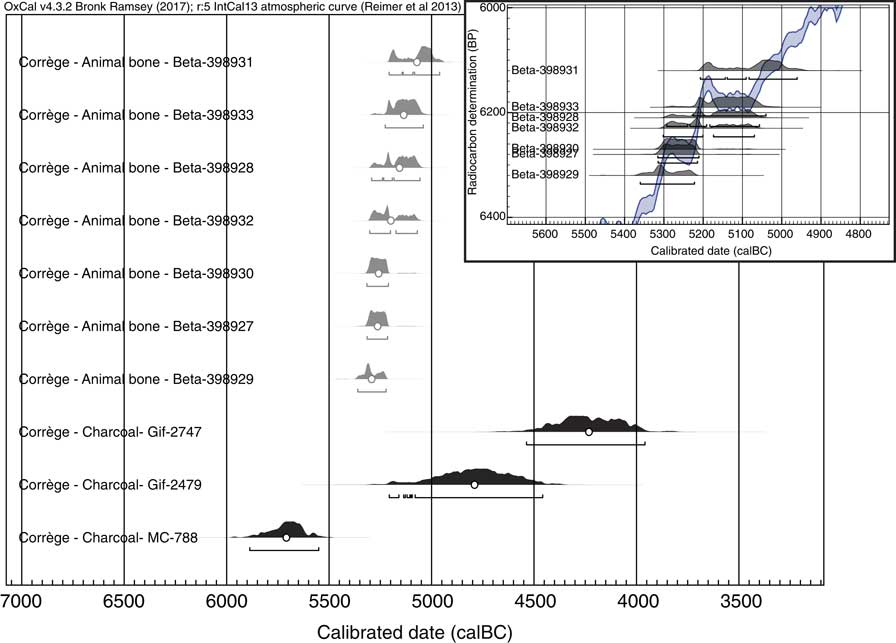
Three dates were made on charcoal gathered from zones with a concentration of objects (Gif-2747, Gif-2748, and Gif-2749), and one on a fragment of waterlogged wood (MC-788). The archaeological link is thus very tenuous for these measurements, which are also incoherent. In addition, they were made on long-lived samples and are affected by high standard deviations. In order to attempt to specify the site chronology, and in spite of the constraints related to the fact that the available samples are decontextualized, our choice focused on five faunal bones associated with Cardial pottery when they were discovered and on two bone tools. The faunal samples are made up of domestic taxa (sheep/goat and bovine). The tools are two awls shaped on deer metapodials. The collagen of all these samples was sufficiently well conserved and ample to obtain consistent results, in spite of their long immersion in a marine environment (Table 1). A first examination of these dates shows that they are regularly spread out in time, ranging between 5350 and 5000 cal BCE (Figure 7). In the absence of stratigraphic observations, it is not possible to define the constraints a priori on the number of occupations recorded by this material, nor any possible spatial organization. The new measurements can thus only be assessed together. The presence of a plateau spanning the whole 52nd century BCE tends to artificially accentuate the downward spreading of the dates.
Calibrated probability distribution of radiocarbon dates from La Corrège OxCal v 4.3.2 Bronk Ramsey (Reference Bronk Ramsey2017); r:5 and IntCal13 atmospheric curve (Reimer et al. Reference Reimer, Bard, Bayliss, Beck, Blackwell, Ramsey, Buck, Cheng, Edwards, Friedrich, Grootes, Guilderson, Haflidason, Hajdas, Hatté, Heaton, Hoffmann, Hogg, Hughen, Kaiser, Kromer, Manning, Niu, Reimer, Richards, Scott, Southon, Staff, Turney and van der Plicht2013). In gray, short-lived samples and dates obtained by AMS; in black, conventional methods of radiocarbon dating on long-lived samples (the Gif-2748 date is not given here as it is much more recent). On the top, curve plot of the seven dates obtained on short-lived samples showing the plateaus effect on the spread of each calibrated date.
Pont de Roque-Haute
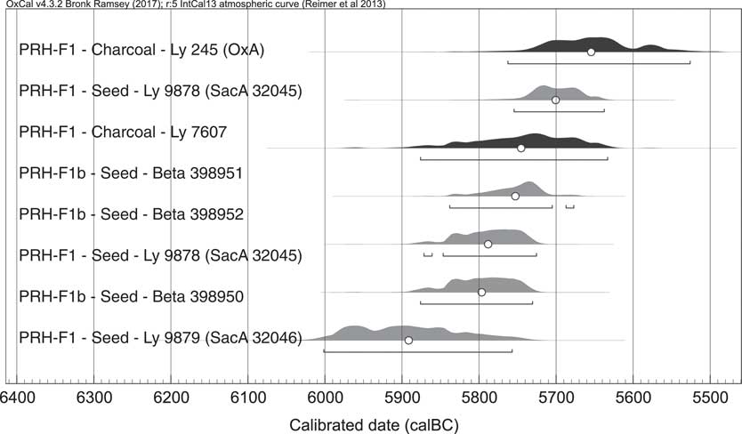
Pont de Roque-Haute is an open-air site made up of several pits, probably associated with a dwelling now eroded by modern farming activities. It is located 1.7 km from the present-day shore of the Mediterranean in the Hérault department (Figure 1). The site was excavated in 1995 by Guilaine. The excavation identified 10 hollow structures truncated by ploughing, comprising a secondary backfill of discarded waste. The latter contained abundant daub fragments belonging to construction walls destroyed by a violent fire (a mixture of earth, sand and straw on a wooden frame), pottery, faunal remains and macro-tools. All these elements indicate well-mastered agro-pastoral practices (Guilaine et al. Reference Guilaine, Manen and Vigne2007) and clear links with the Ceramica Impressa from southern Italy. The presence of obsidian from Palmarolla at the site reinforces these links. A first series of dates on unspecified charcoal carried out after the excavation yielded two coherent, statistically identical results, between 5770 and 5620 cal BCE (Ly-7607 and Ly-245-Ox). These dates made Pont de Roque-Haute one of the oldest Neolithic sites in the Western Mediterranean. In order to confirm these results and to circumvent discussions concerning a potential old wood effect, we selected five new short-lived samples (cereal seeds) from pit 1 (F1), which contains the most artifacts (Table 1). All belong to emmer (Triticum dicoccum). These five new dates totally confirm the early age of this occupation, and four of them are even older than the dates obtained on charcoal (Figure 8). All of these seven dates can thus be retained to discuss the settlement chronology of the site. Two clusters can be statistically differentiated on the basis of the Chi2 test. The dates Ly-7607, Beta-398952, Beta-398951, Beta-398950, and Ly-9879 are statistically identical (χ2=4.78, df=4, α[5%]=9.4). The dates Ly-245 and Ly-9878 are statistically identical (χ2=0.82, df=1, α[5%]=3.8). The Bayesian modeling of these results (Figure 9) grouped together according to two successive events (base of pit 1 below F1) belonging to a single phase enables us to propose the hypothesis of a short occupation, with a duration of about 80 years (MAP value; HPD region: 0–310 years [95%]), between 5780 (MAP value; HPD region: 5960–5710 cal BCE [95%]) and about 5720 cal BCE (MAP value; HPD region: 5790-5540 cal BCE [95%]; Table 4).
Calibrated probability distribution of radiocarbon dates from Pont de Roque-Haute. OxCal v 4.3.2 Bronk Ramsey (Reference Bronk Ramsey2017); r:5 and IntCal13 atmospheric curve (Reimer et al. Reference Reimer, Bard, Bayliss, Beck, Blackwell, Ramsey, Buck, Cheng, Edwards, Friedrich, Grootes, Guilderson, Haflidason, Hajdas, Hatté, Heaton, Hoffmann, Hogg, Hughen, Kaiser, Kromer, Manning, Niu, Reimer, Richards, Scott, Southon, Staff, Turney and van der Plicht2013). In gray, short-lived domestic samples; in black, long-lived samples dated by AMS.
Bayesian model of Pont de Roque-Haute (events on the left part of the diagram, phases on the right; ChronoModel 2.0.4). At the bottom, posterior density distribution of the model. The density regions of the beginnings are the oldest. The areas below the curves represent the 95% highest posterior densities. Arrows indicate the stratigraphic constraints applied to the successive events.
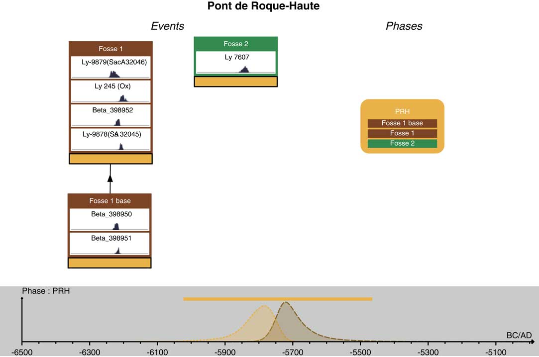
At the top: modeled events of Pont de Roque-Haute. The number of associated dates is for each event indicated in brackets; e_HPD (95%), i.e. event’s highest posterior density interval at 95% confidence; e_MAP, event’s posterior mode. At the bottom: modeled phases of Pont de Roque-Haute. The number of associated events and dates for each event is indicated in brackets: D_HPD (95%), highest posterior density interval at 95% confidence of phase duration; D_MAP, posterior mode of phase duration; B_HPD (95%), highest posterior density interval at 95% confidence of phase beginning; B_MAP, posterior mode of phase beginning; E_HPD (95%), highest posterior density interval at 95% confidence of phase’s end; E_MAP, posterior mode of phase’s end.

Peiro Signado
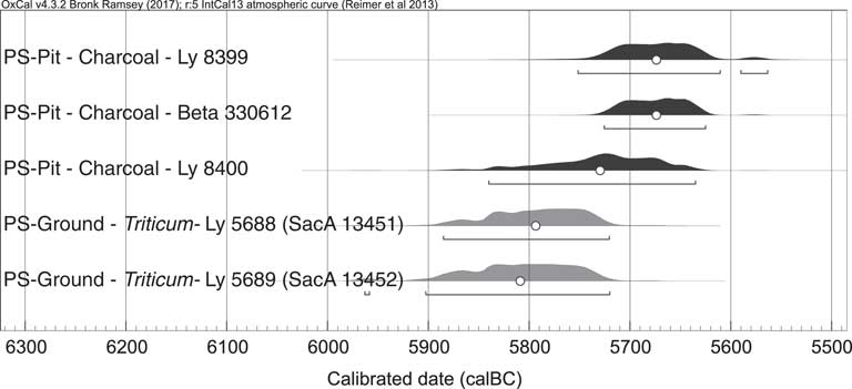
Peiro Signado, located in the same municipality of Portiragnes in the Hérault, is also an open-air site installed on a small promontory overhanging the Orb Valley (Figure 1). It was excavated between 1977 and 1978 by Roudil, then between 1996 and 1997 by Briois. The 1996-1997 excavation seasons resulted in the identification and the excavation of the whole conserved surface of the site, extending over nearly 100 m2. The site is organized into two poles (Briois and Manen Reference Briois and Manen2009): a sector of pits and a ground level. The pits may have been used for extracting clay to make pottery or for the daub. The ground level is surrounded by eight post holes. It was thus possible to reconstruct an oval-shaped or polygonal edifice of about 70 m2. The associated objects are extremely abundant and diversified (pottery, flint tools, fragments of obsidian from Palmarolla and Sardinia). The bones are very poorly preserved, but the carpological analysis provides evidence of farming practices by the cultivation of emmer wheat (Triticum dicoccum). After the 1978 excavation, a first date was made on a charcoal sample (MC-1652). This yielded a result with a high standard deviation, and inconsistent with the archaeological series. Five new dates were then made on the material from the 1996 and 1997 excavations. Charcoal and charred seeds were selected from the sector of the pits and the archaeological ground (Table 1). First of all, we note that the dates on charcoal are slightly more recent than those on caryopses of emmer (Figure 10). It is not possible to organize these measurements according to the stratigraphy, as they come from the occupation floor on one hand (Ly-5688 and Ly-5689), and the fill of the adjacent pits on the other (Ly-8399, Ly-8400, and Beta-330612). These five dates are thus related to three archaeological entities (pits F1 and F7, floor), which represent as many events in Bayesian modeling, with no stratigraphic limits between them (Figure 11). All are related to the same unique phase. This is situated between 5800 (MAP value; HPD region: 5920–5710 cal BCE [95%]) and 5660 cal BCE (MAP value; HPD region: 5750–5550 cal BCE [95%]; Table 5). The duration of this occupation is estimated at 140 years (MAP value; HPD region: 30–300 years [95%]). Like Pont de Roque-Haute, Peiro Signado records one of the oldest Neolithic occupations in the Western Mediterranean and is related to Italian, and more specifically, Ligurian cultural contexts.
Calibrated probability distribution of radiocarbon dates from Peiro Signado. OxCal v 4.3.2 Bronk Ramsey (Reference Bronk Ramsey2017); r:5 and IntCal13 atmospheric curve (Reimer et al. Reference Reimer, Bard, Bayliss, Beck, Blackwell, Ramsey, Buck, Cheng, Edwards, Friedrich, Grootes, Guilderson, Haflidason, Hajdas, Hatté, Heaton, Hoffmann, Hogg, Hughen, Kaiser, Kromer, Manning, Niu, Reimer, Richards, Scott, Southon, Staff, Turney and van der Plicht2013). In gray, short-lived domestic samples; in black, long-lived samples dated by AMS.
Bayesian model of Peiro Signado (events on the left part of the diagram, phases on the right; ChronoModel 2.0.4). At the bottom, posterior density distribution of the model. The density regions of the beginnings are the oldest. The areas below the curves represent the 95% highest posterior densities. As there are no stratigraphical links between the different structures, no stratigraphical constraints are drawn. The MC-1652 date, which is not correctly referenced, is not taken into account in the model.

At the top: modeled events of Peiro Signado. The number of associated dates is for each event indicated in brackets; e_HPD (95%), i.e. event’s highest posterior density interval at 95% confidence; e_MAP, event’s posterior mode. At the bottom: modeled phases of Peiro Signado. The number of associated events and dates for each event is indicated in brackets: D_HPD (95%), highest posterior density interval at 95% confidence of phase duration; D_MAP, posterior mode of phase duration; B_HPD (95%), highest posterior density interval at 95% confidence of phase beginning; B_MAP, posterior mode of phase beginning; E_HPD (95%), highest posterior density interval at 95% confidence of phase’s end; E_MAP, posterior mode of phase’s end.
Taï
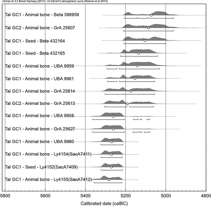
The site of Taï is located in the municipality of Remoulins, in the Gard, at the eastern limit of the garrigues of Nîmes (Figure 1). It is situated in one of the small valleys carving into the limestone plateau overlooking the Gardon and opening onto the plain of Remoulins. It is thus positioned at the junction of different ecosystems conducive to the implantation of Neolithic societies (plateaus, steep slopes, plain, etc.). It was excavated between 2001 and 2012 by Manen (Manen et al. Reference Manen, Bouby, Carrère, Coularou, Devillers, Muller, Perrin, Sordoillet, Vigne and Voruz2004; Caro and Manen Reference Caro and Manen2014). The site was made up of two karstic openings opposite each other and an open-air area more or less circumscribed by the ledge. Many successive occupations have been identified, from the Early Neolithic to the Early Bronze Age. The Early Neolithic sequence was subdivided into two levels at the excavation (GC1 and GC2), although it is not possible to observe any visible occupation discontinuity between them (Figure 12). We can thus consider that the occupation and/or the use of the cave during the Early Neolithic occurred with no real interruption and that only functional changes in the different sectors can be observed throughout time. This hypothesis of a continuous occupation of the site, during the Early Neolithic, is confirmed by the components of the technical system (material production and faunal remains). They are related to the Epicardial cultural facies. The site formation and assemblage integrity has been tested through geoarchaeological analyses and potsherds refitting (Caro and Manen Reference Caro and Manen2014) and the sampling strategy was based on these data. Fourteen AMS dates were carried out on short-lived samples (non-heated faunal bones and charred seed) from both levels. The reliability of one of these measures may be discussed because of the value of the δ13C (UBA9960). The Bayesian modeling (Figure 13) shows that the first occupations of the site took place towards 5300 cal BCE (MAP value of the beginning of GC1; HPD region: 5400–5230 cal BCE [95%]; Table 6). They end towards 4980 cal BCE (end MAP value of GC2; HPD region: 5130–4550 cal BCE [95%]) All in all, the Epicardial horizon of Taï is dated between about 5300 and 5000 cal BCE.
Calibrated probability distribution of radiocarbon dates from Le Taï. OxCal v4.3.2 Bronk Ramsey (Reference Bronk Ramsey2017); r:5 and IntCal13 atmospheric curve (Reimer et al. Reference Reimer, Bard, Bayliss, Beck, Blackwell, Ramsey, Buck, Cheng, Edwards, Friedrich, Grootes, Guilderson, Haflidason, Hajdas, Hatté, Heaton, Hoffmann, Hogg, Hughen, Kaiser, Kromer, Manning, Niu, Reimer, Richards, Scott, Southon, Staff, Turney and van der Plicht2013).
View of the lower part of the Bayesian model for Le Taï (events on the left part of the diagram, phases on the right; ChronoModel 2.0.4). At the bottom, posterior density distribution of this part of the model. The density regions of the beginnings are the oldest. The areas below the curves represent the 95% highest posterior densities. Arrows indicate the stratigraphic constraints applied to the successive events or phases.

At the top: modeled events of Le Taï. The number of associated dates is for each event indicated in brackets; e_HPD (95%), i.e. event’s highest posterior density interval at 95% confidence; e_MAP, event’s posterior mode. At the bottom: modeled phases of Le Taï. The number of associated events and dates for each event is indicated in brackets: D_HPD (95%), highest posterior density interval at 95% confidence of phase duration; D_MAP, posterior mode of phase duration; B_HPD (95%), highest posterior density interval at 95% confidence of phase beginning; B_MAP, posterior mode of phase beginning; E_HPD (95%), highest posterior density interval at 95% confidence of phase’s end; E_MAP, posterior mode of phase’s end.
DISCUSSION
This new series of dates brings new insights into the main problems regarding the Neolithic transition in the Western Mediterranean.
Taphonomic and Methodological Perspectives
First of all, from a methodological point of view, this dating programme generates comments regarding practices for the construction of reliable chronological frameworks. It is possible to observe that a precise protocol of sample selection for dating, based on a multi-proxy reassessment of the chrono-stratigraphy, allows us to reconsider formerly excavated sites, even if the excavations were carried out some time ago (Barshay-Szmidt et al. Reference Barshay–Szmidt, Costamagno, Henry-Gambier, Laroulandie, Pétillon, Boudadi–Maligne, Kuntz, Langlais and Mallye2016; Perrin et al. Reference Perrin, Manen, Valdeyron and Guilaine2017).
The choice of samples to be dated should clearly focus on short-lived samples. Measurements obtained in the past on charcoal can no longer form the basis of discussions on the spatio-temporal dynamics of Neolithisation. The examples of Camprafaud and Aigle are particularly relevant (Figures 2 and 5). The measurements taken in the 1980s on charcoal using the conventional method (risk of mixing different charcoals) are affected on one hand by very high standard deviations, and on the other by a clear “old wood” effect. In the case of Camprafaud, these results contributed to the discussion on a “native Neolithisation”, a controversial debate that turned out for this site (and for others Perrin et al. Reference Perrin, Manen, Valdeyron and Guilaine2017) to be based on a poor archaeological link between the date and the human event in question. Nonetheless, these observations must be moderated by noting that the dates on single charcoal fragments are not systematically affected by this old wood effect. The two sites of Peiro Signado and Pont de Roque-Haute are good demonstrations of this: in both cases, the dates obtained on cereal seeds are older than those obtained on charcoal (Figures 8 and 10). It thus seems that the systematic rejection of dates carried out by AMS on charcoal is not a priori systematically justified, even if each series obtained on charcoal must be critically examined.
The new measurements published here were made on short-lived samples: mainly non-heated animal bones, charred seeds, and fruits. All of these materials are directly linked to human activities. Most of the seeds and more than half of the bones belong to domestic species and are products of farming. It is important to underline the coherent results obtained on bone industry from the site of La Corrège, a Cardial occupation with no stratigraphic context. With this relatively non-intrusive practice, it is possible to overcome the problem of the archaeological link in this type of context and to validate the other measurements obtained on consumed animal bones.
The analysis of the spatio-temporal dynamics of Neolithisation is frequently based on the dating of domestic plants and animals (Capra hircus, Ovis aries, and Cerealia). But, in some cases, these samples are rare in the assemblages and it seems to be a shame to omit the measurements obtained on wild taxa from our considerations. At Balma Margineda, for example, two measurements taken on a cereal seed and a hazelnut shell give statistically identical results. We now know that wild resources are important for Early Neolithic communities in the South of France and in Spain (Vigne Reference Vigne2007; Rowley-Conwy et al. Reference Rowley-Conwy, Gourichon, Helmer and Vigne2013; Saña Reference Saña Segui2013; Antolin Reference Antolín2015), and omitting these data or attributing them to Mesolithic behaviour considerably reduces our field of reflection.
Another major problem related to the problem of transitions, and in particular the Neolithic transition, is that of stratigraphic mixing (Guilaine Reference Guilaine1993; Bernabeu Aubán et al. Reference Bernabeu Aubán, Barton and Perez Ripoll2001), particularly in sites occupied for long periods of time. The example of Gazel Cave shows that the domestic sheep bones found in the Second Mesolithic horizons were not in primary position and that the hypothesis of interactions between the last hunters and the first farmers is overturned, at least at this site. In all the contexts under consideration from this point of view, it is essential to proceed with the direct dating of the remains in order to form solid foundations for reflections.
Lastly, it is important to underline that the calibration curve shows a series of oscillations (plateau and slope discontinuity) generating multiple solutions during the calibration of dates between 6250 and 6000 BP, or roughly during the period 5300–5000 cal BCE (example of Leucate, Figure 7), or the expansion phase of the Cardial and the genesis of the Epicardial. It is important to take these curve oscillations into account as they cause an increase in calibration imprecision through the plateaus themselves, but they can also cause artificial ruptures in continuous sequences. Indeed, the date of an event is limited by the beginning and the end of the calibrated ranges, values that must not be considered as a duration, but as a terminus post quem and ante quem surrounding the true date, which is somewhere between these two limits, up to the limits of the plateau itself. The multiplication of dates thus leads to a recurrence in the value of the limits, creating a misleading impression of a “threshold” date. This is the case for the Early Neolithic with the dates of 5300 or 5200 cal BCE. The probability that these cultural changes identified in 5300 cal BCE really occurred at this date is thus more or less non-existent, and it is important to note that the chronological precision for the whole period 5300–5100 cal BCE is very low and could not be resolved by radiocarbon dating. Bayesian modeling can provide several supplements, but the dispersal of modeled dates in a plateau remains intrinsically artificial. This problem thus represents a genuine bias in our understanding of this period of major economic and cultural reconfiguration.
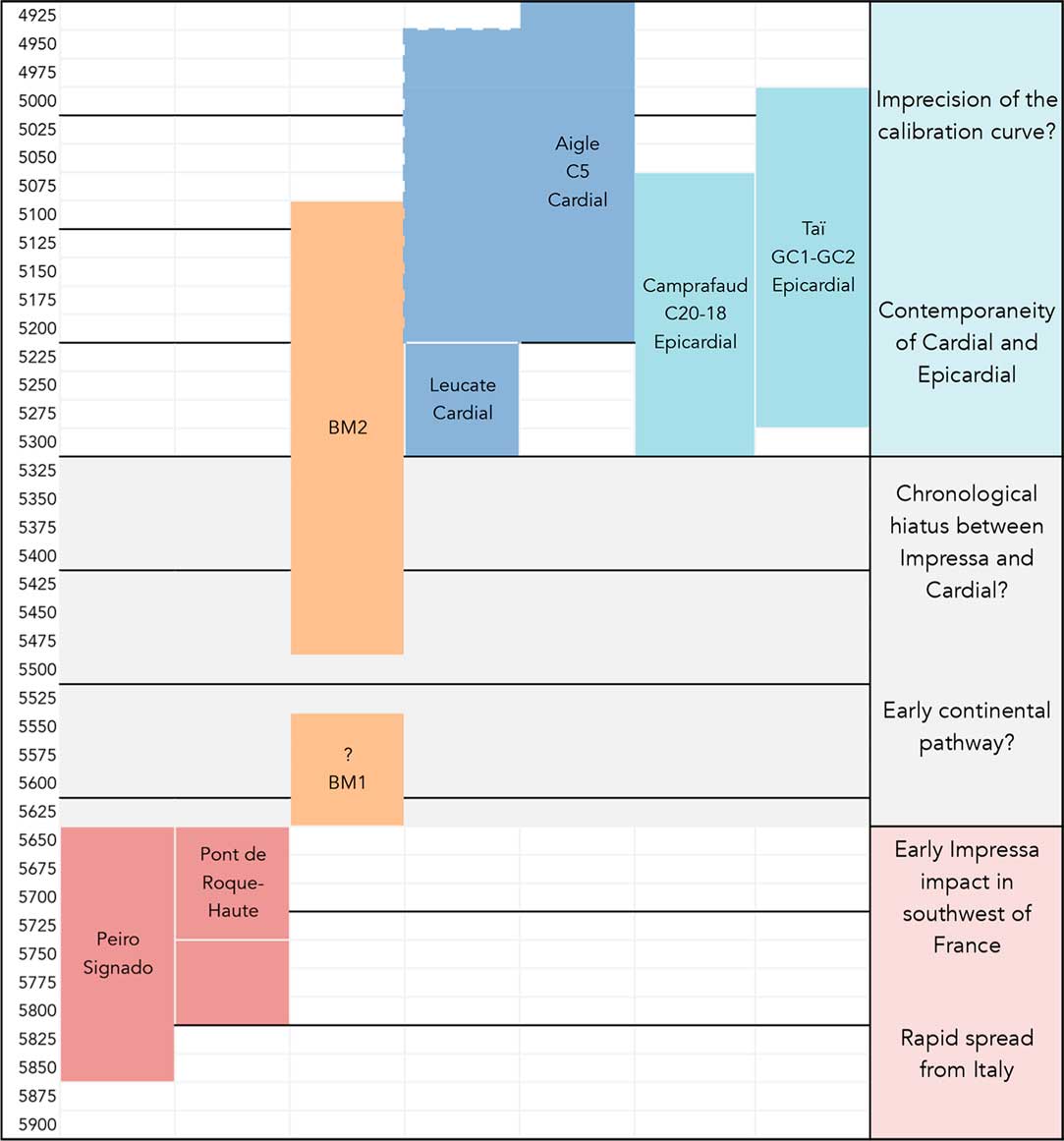
These methodological considerations aside, this new chronometric framework enables us, on one hand, to refine the regional chronological sequences of the Neolithisation of the South of France (Figure 14) and, on the other, to discuss the nature of this process on a wider Western Mediterranean scale. Indeed, based on these new-modeled dates, we are able to address the main issues of the Western Mediterranean Neolithisation (i.e. the speed of expansion and the spatio-temporal development of the first farmers).
Schematic representation of the new regional chronological sequences (i.e. based on the results of the modeling of each site) from the southwest of France and of their main contributions to Western Mediterranean Neolithisation issues.
Pioneering Impressa Systems
Evidence from the sites of Peiro Signado and Pont de Roque-Haute reveals the development of perfectly mastered exogenous Neolithic technical and economic systems. New dates confirm the early age of these first Neolithic impacts on the French coast. Indeed, there is very little discrepancy (Figure 15) between the earliest dates obtained on short-lived samples in southern Italy (Trasano, Favella, and Ripa Tetta; Binder et al. Reference Binder, Angeli, Gomart, Guilaine, Manen, Maggi, Muntoni, Panelli, Radi, Tozzi, Arobba, Battentier, Brandaglia, Bouby, Briois, Carré, Delhon, Gourichon, Marinval, Nisbet, Rossi, Rowley-Conwy and Thiébault2017), on the Adriatic coast (Rasinovac and Pokrovnik) and in Liguria and those from Portiragnes, where the whole technical system is related to the Ceramica Impressa cultural sphere (no dates made on short-lived samples are available for the Tyrrhenian zone before 5750 cal BCE).
Map of the Western Mediterranean sites where samples with short life cycles were dated between 5900 and 5750 cal BCE. Weighted cumulative histograms of the radiocarbon dates made on short-lived samples, see Supplementary Appendix 1).

Therefore, these data diverge from the hypothesis of a progressive and regular diffusion of the Neolithic economy, which is sometimes perceived at a European scale (Ammerman and Cavalli-Sforza Reference Ammerman and Cavalli–Sforza1971 for the princeps model and Pinhasi et al. Reference Pinhasi, Fort and Ammerman2005, for example). There is no confirmation of this “wave of advance” model in the spatial and temporal dynamics of the Western Mediterranean, which reflects more of a discontinuous process. Moreover, insofar as seafaring movements are probably involved (Isern et al. Reference Isern Sardó, Zilhao, Fort and Ammerman2017), and as the rhythm of diffusion varies considerably from one point to another in this area, it appears illusory to estimate the average speed of propagation of the first farming communities and to draw conclusions on the nature of diffusion. In actual fact, we have no idea of the route followed by these communities and the geographic discontinuities are still much too significant to advance a credible wide scale model.
The two Languedoc sites of Peiro Signado and Pont de Roque-Haute thus probably provide evidence of long-distance maritime movements, but with a low transformation of technical and economic traditions (Manen and Convertini Reference Manen and Convertini2012). These pioneers kept the way of life and technical traditions developed in the zone of origin, and at the same time adapted to regional environmental characteristics and used the diversity of resources available (particularly for the lithic industries and pottery productions). This process, described as pioneering, is not dissimilar to the “two-stage model” advanced for the Adriatic where Forenbaher and Miracle (Reference Forenbaher and Miracle2005) link the dispersal of the first farmers with maritime movement and exploratory behavior. In the Western Mediterranean, early incursions towards the islands, evidenced by the use of obsidian from Sardinia and Palmarola (found at Pont de Roque-Haute and Peiro Signado; Briois et al. Reference Briois, Manen and Gratuze2009), and rapid long-distance movements could reinforce this model. The future of these pioneering groups and their impacts on the overall Neolithisation process in the South of France and possibly in Mediterranean Spain, are still difficult to gauge (Guilaine and Manen Reference Guilaine and Manen2007; Bernabeu Aubán and Martí Oliver Reference Bernabeu Aubán and Martí Oliver2014).
Chronology of the Cardial Complex
A second phase marks the development of the Cardial complex, the vector of the full development of the Neolithic economy in a lot of the Western Mediterranean. In the South of France (Figure 16) the examination of the newly acquired data and the data available for Provence (dates with low standard deviations made on short-lived samples, Binder and Sénépart Reference Binder and Sénépart2010), shows that this Cardial culture does not begin before 5450 cal BCE on the French coast, thus calling into question the periodizations established in the 1990s–2000s (hypothesis of an early chronology starting towards 5600/5500 cal BCE: Manen and Guilaine Reference Manen and Guilaine2010). This revision of the chronometric framework of the Cardial culture thus raises several points for discussion:
∙ First of all, from a methodological point of view, we must note that this rejuvenation of the beginning of the Cardial culture is clearly linked to the problem of dates carried out on charcoal (old wood effect) and with high standard deviations (i.e. wide calibration range);
∙ Then from a historical point of view, we must underline that there is now a real chronological hiatus for a lot of the South of France between sites with Impressa facies s.l. (Peiro Signado and Pont de Roque-Haute type) and those from the Cardial. Given the available data (apart from the sequence of Pendimoun in eastern Provence, at the Italian border; Binder et al. Reference Binder, Angeli, Gomart, Guilaine, Manen, Maggi, Muntoni, Panelli, Radi, Tozzi, Arobba, Battentier, Brandaglia, Bouby, Briois, Carré, Delhon, Gourichon, Marinval, Nisbet, Rossi, Rowley-Conwy and Thiébault2017), and if we only retain dates obtained on short-lived samples with a low standard deviation, no sites are dated between 5600 and 5400 BCE.
Two hypotheses can be advanced:
∙ Hypothesis 1: this situation reflects an archaeological reality that could be related to the model of micro-breaks (Guilaine Reference Guilaine2013) observed in the Neolithic diffusion in the Mediterranean at different periods and in diverse places. The reasons behind this break are still unknown for now.
∙ Hypothesis 2: this situation only represents an artifact of research linked to a lack of data for the initial phases of the Cardial culture.
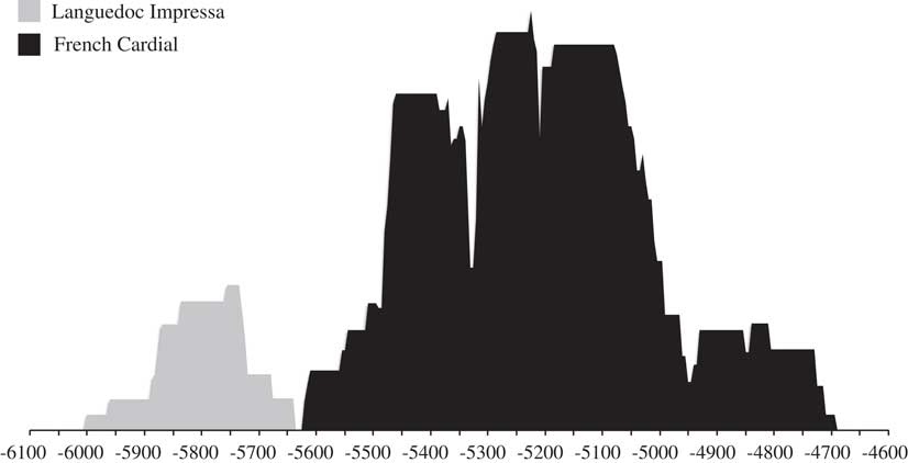
Cumulative weighted histograms of the radiocarbon dates from the Impressa sites of Languedoc (Peiro Signado and Pont de Roque-Haute) and the sites of the French Cardial complex (short-lived samples, see Supplementary Appendix 2).
If we broaden the focus to consider the data from eastern Provence and the Iberian Peninsula (Figure 17), we can observe that several sites yield dates ranging between 5600–5400 BCE. Yet the Spanish Cardial is traditionally considered to originate in the South of France. Can we thus consider that the chronological gap mentioned above is just linked to the state of current research? Or must we also call into question this alleged affiliation between the French and Spanish Cardial? Lastly, we must mention the strong climatic deteriorations with erosive capacity, including a major deterioration towards 5400 cal BCE, identified in the South of France and which could have contributed to the disappearance of early Cardial sites (Berger Reference Berger2006).
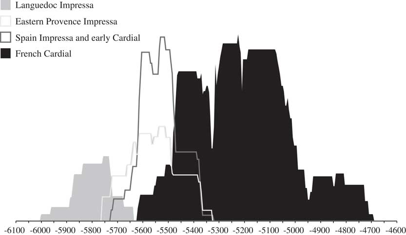
Cumulative weighted histograms of the radiocarbon dates from the Impressa sites of Languedoc and Eastern Provence, the Impressa and Early Cardial sites of Spain and of the French Cardial complex (short-lived samples, see Supplementary Appendix 3).
Early Continental Pathway?
At a regional scale, it is traditionally accepted that the coast was settled early on by the first Neolithic communities, whereas continental and mountain incursions occurred later on. The new data acquired in the scope of the Procome project propose to revise this model. The dates obtained for the site of Balma Margineda (BM1 and BM2) show that there is only a 200-year gap between this site and the well-identified occurrences on the coast (Figure 14), not a long time lag as has been previously argued. In addition, the presence of shellfish of Mediterranean origin transformed into ornaments clearly shows the connection of the site with the coastal zone. No Neolithic sites dated between 5650 and 5550 cal BCE are known in the immediate environment of Balma Margineda, but the recent identification of indirect indicators of anthropization in the municipality of Canohès (about 150 km away by the valley of the Têt and the Conflent) opens new avenues of research (Manen et al. in Reference Manen, Carozza, Marchand and Perrinpress). Other markers of early human presence in the mountains have been mentioned on the sole basis of the early dates from the valley of Madriu-Perafita-Claror (Orengo et al. Reference Orengo, Palet Martinez, Ejarque Montolio, Miras and Riera Mora2014), several kilometers from Balma Margineda, or at la Cova del Sardo (Sant Nicolau valley; Gassiot et al. Reference Gassiot Ballbé, Pèlachs Mañosa, Bal, García Díaz, Julià Bruguers, Pérez Obiol, Rodriguez and Astrou2010). In both cases, the dates were measured on charcoal (KIA-37689: 6525 ± 45 BP for the hearth A-9B1/a, giving 5565–5375 cal BCE for la Cova del Sardo; 5544 ± 69 cal BCE for Madriu P009110 with no other indication). In the valley of Madriu-Perafita-Claror, the archaeological link is poor; in the case of la Cova del Sardo, the charcoal was sampled in a hearth associated with a sparse and uncharacteristic lithic industry. But these dates are not sufficiently reliable to back up this scenario. The works of D. Galop (Reference Galop2006), based on paleoenvironmental approaches by coring, show the repeated opening of the forest environment, sometimes at early dates. But again, much work remains to be done to back up these hypotheses and give these markers a solid archaeological contextualization. In the same line of thought, we observe that among the earliest Cardial sites from the South of France and the northeast of the Iberian Peninsula, those of Baume de Montclus, Baume d’Oullins, Baume de Ronze or Cova de Chaves give the earliest dates on domestic samples (Fernandez et al. Reference Fernandez, Hughes, Vigne, Helmer, Hodgins, Miquel, Hanni, Luikart and Taberlet2006; Garcia-Martinez de Lagran Reference García Martínez de Lagrán2014). Yet these sites are located over one hundred kilometers from the present-day shoreline. Finally, let us note that in the history of research into Mediterranean Neolithisation, efforts have undeniably concentrated on coastal zones (as have major development works leading to preventive excavations). It now seems important to address this specific issue and to get more reliable data to confirm the two dates obtained at Balma Margineda.
Cultural Diversity and Change
Cardial and Epicardial are two facies, mainly differentiated on the basis of their pottery production (differences in the treatment of raw materials and decorative techniques, Manen et al. Reference Manen, Sénépart and Binder2010), which develop in southern France during the second half of the 6th millennium. There are two main models that have been proposed to address this duality: a cultural filiation between Cardial and Epicardial (and thus a chronological evolution); or a “peripheralisation or functional differentiation” process of two contemporary groups. The renewed chronological framework enables us to confirm, at least partially, the “contemporaneity” between the two Early Neolithic facies from the South of France: Cardial and Epicardial (Figure 14). The new dates obtained show a wide range of overlapping between the two, during the last centuries of the sixth millennium BCE. These observations call for two comments. First of all, we must question the reality of this long period of contemporaneity suggested by the radiocarbon record. In fact, the time range during which these two facies develop simultaneously corresponds exactly to that of significant oscillations in the calibration curve (cf. above). As a result, the chronological precision obtained by the radiocarbon dates, which are the only ones we have for this period, does not provide any decisive arguments on this question. This contemporaneity is possible, and even very probable, but cannot be objectively demonstrated with this method. However, the detailed analysis of the technical systems confirms this hypothesis (although it cannot clarify the time range), as it is possible to observe interactions and reciprocal transfers of techniques and/or finished products (particularly pottery) between the two technical traditions. Therefore, the hypothesis of a simple chronological sequence with no overlapping can no longer be upheld for the Cardial and the Epicardial, and a period of overlap between the two must now be acknowledged. The range of this overlap has yet to be determined but was sufficiently long to allow for exchanges and transfers. The anthropological aspects of this coexistence must now be questioned and documented, with particular emphasis on the questions of settlement dynamics and the factors driving cultural change. This represents the main challenge for future works on the Early Neolithic in the South of France.
CONCLUSIONS
To conclude, we will highlight two main points:
∙ It is now clear that the development of Neolithic transition scenarios cannot be dissociated from a revised chronometric framework based on adapted and updated protocols (Wood Reference Wood2015), as demonstrated by recent overviews of diverse geographic areas (MacClure et al. Reference McClure, Podrug, Moore, Culleton and Kennett2014; Martins et al. Reference Martins, Oms Arias, Pereira, Pike, Rowsell and Zilhão2015; Garcia Puchol et al. Reference Garcia-Puchol, McClure, Juan-Cabanilles, Bernabeu Aubán, Marti-Oliver, Pardo-Gordo, Pascual Benito, Pérez-Ripoll, Molina Balaguer and Kennett2017; Binder et al. Reference Binder, Angeli, Gomart, Guilaine, Manen, Maggi, Muntoni, Panelli, Radi, Tozzi, Arobba, Battentier, Brandaglia, Bouby, Briois, Carré, Delhon, Gourichon, Marinval, Nisbet, Rossi, Rowley-Conwy and Thiébault2017). In turn, the new data from the PROCOME program emphasize the importance of a sampling strategy based on “archaeological link” criteria (i.e., taphonomic filter) and on radiocarbon events (short-lived samples). It also appears important to obtain sufficient dates for each “event” to test the representativeness of the obtained measurements. In spite of that, radiocarbon precision is still unsatisfactory for assessing specific events or more generally, for a detailed chronological linking of the different sites.
∙ Like all the data used for prehistoric archaeology, the radiocarbon dates cannot be studied solely for their intrinsic value, without detailed contextualization (archaeological context, local and regional taphonomy). It is illusory, as well as methodologically very questionable, to believe that the number compensates for inconsistencies or poor links. It also does not make much sense to study the radiocarbon dates without comparing them to other proxies (material productions, subsistence economy…). If we superimpose data from the characterization of technical systems with audited and contextualized radiocarbon data, it becomes possible to bring to light complex and multi-faceted processes of the emergence and development of the Neolithic economy and to deliver a much more informative historical narrative.
Unlike global models established at a continental scale, the renewed data for the Western Mediterranean bring to light complex and much less unidirectional processes of diffusion than those considered up until now. Maritime diffusion can, for example, be marked by pause intervals, whereas conversely, mainland settlement may have occurred early on. This shows the importance of testing general models with local scales (Gkiaska et al. 2003; Bernabeu Aubán et al. Reference Bernabeu Aubán, Barton, Pardo Gordó and Bergin2015) in order to reconstruct the richness and variety of Neolithic transition scenarios.
ACKNOWLEDGMENTS
This work was supported by the ANR (The French National Agency for Research) within the framework of the program CULT (Metamorphosis of societies – Emergences and evolution of cultures and cultural phenomena; ANR-13-CULT-0001-01). It has been undertaken within the PROCOME Project “Continental extension of the of the Mediterranean Neolithization”. C. Manen, T. Perrin wrote the paper and made the radiocarbon data analysis. J. Guilaine, C. Manen and F. Briois provided new stratigraphic and cultural data. S. Bréhard, L. Bouby, F. Durand, P. Marinval and J.-D. Vigne identified the zoological and botanical samples and made up the protocol of selection of samples with C. Manen. This manuscript has been improved and approved by all co-authors.
Supplementary materials
To view supplementary material for this article, please visit https://doi.org/10.1017/RDC.2018.98


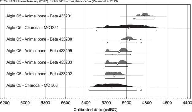


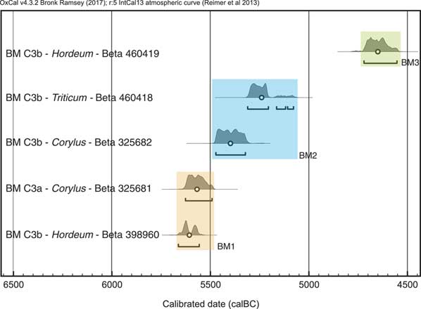

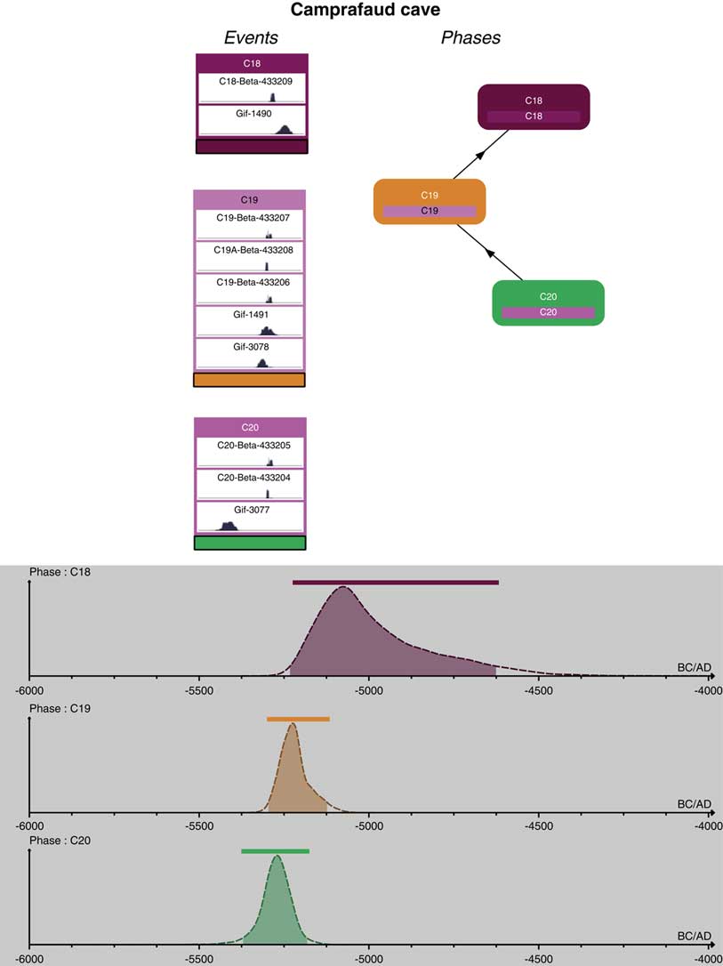


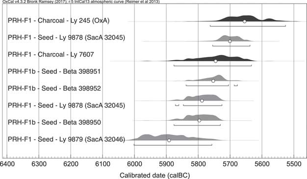


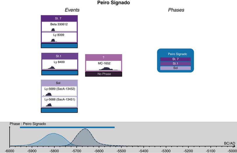


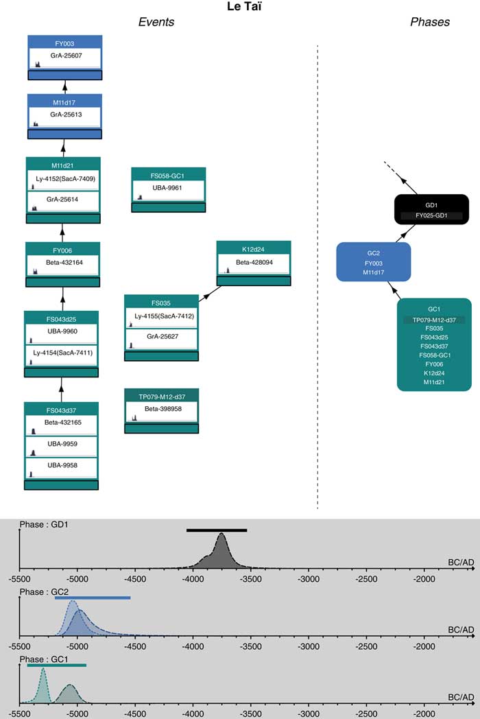


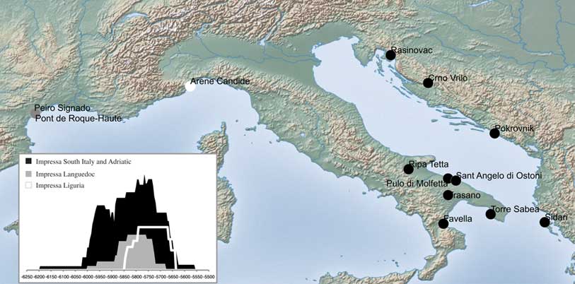

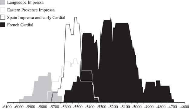


 Open access